Qudit inspired optimization for graph coloring
Abstract
We introduce a quantum-inspired algorithm for Graph Coloring Problems (GCPs) that utilizes qudits in a product state, with each qudit representing a node in the graph and parameterized by -dimensional spherical coordinates. We propose and benchmark two optimization strategies: qudit gradient descent (QdGD), initiating qudits in random states and employing gradient descent to minimize a cost function, and qudit local quantum annealing (QdLQA), which adapts the local quantum annealing method to optimize an adiabatic transition from a tractable initial function to a problem-specific cost function. Our approaches are benchmarked against established solutions for standard GCPs, showing that our methods not only rival but frequently surpass the performance of recent state-of-the-art algorithms in terms of solution quality and computational efficiency. The adaptability of our algorithm and its high-quality solutions, achieved with minimal computational resources, point to an advancement in the field of quantum-inspired optimization, with potential applications extending to a broad spectrum of optimization problems.
I Introduction
Today, many prominent tasks in industry can be formulated as integer optimization problems, such as how to efficiently use resources kallrath2005solving or do tasks like job scheduling ku2016mixed or portfolio optimization he2014two . One important example of integer optimization is the graph coloring problem (GCP): given a graph with nodes and edges, assign colors to the nodes such that no two connected nodes share the same color. More generally, one might try to find the minimum number of colors needed for such an assignment to be possible, henceforth referred to as the chromatic number of a graph lewis_16 . Being NP-Complete garey1974some , the GCP can be related to a large number of real-world problems, including air traffic control barnier_14 , charging electric vehicles deller_23 , resource allocation (e.g. supply-chain or portfolio management), even tasks like designing timetables, seating plans, sports tournaments or sudoku lewis_16 . Thus, there is much active research in developing algorithms that efficiently find good or optimal solutions to the GCP and scale favourably with the size of the graph.
Quantum technologies might provide one avenue for efficiently solving optimization problems through algorithms like the Quantum Approximate Optimization Algorithm (QAOA) farhi_14 ; hadfield_19 ; oh_19 or quantum annealing hauke_2020 ; pokharel_21 ; yarkoni_2022 . While there is a straight-forward mapping from binary optimization problems to qubit systems lucas_14 ; glover_22 , some integer optimization problems, like GCPs, are more naturally formulated using larger local degrees of freedom. One way to accomplish this in a physics-inspired manner is to extend the notion of a qubit to a -dimensional local degree of freedom, known as a qudit. This, together with the improved capacity for simulations of physical systems with a larger number of local physical degrees of freedom, has inspired the development of hardware implementing qudit systems and qudit-inspired algorithms lu_20 ; wang_20 ; ringbauer_22 . For instance, in Ref. deller_23 , Deller et al. extend QAOA and integer optimization problems, including the GCP, to the qudit regime, and Ref. bottrill_23 explores using qutrits (3-dimensional local degrees of freedom) for the GCP.
Complementary to the improvement of quantum technologies, the connection between quantum physics and optimization problems has enhanced the interest in so-called “physics-inspired algorithms” for optimization. A variety of such algorithms have emerged based on techniques like mean field theory smolin_14 ; veszeli_22 ; bowles_22 , tensor networks bauer_15 ; mugel_22 , neural networks gomes_19 ; Zhao_2021 ; schuetz_22 ; khandoker_2023 , and dynamical evolution Tiunov_19 ; goto_19 ; goto_21 . Some of these new approaches have found significant success, providing state-of-the-art solutions to existing problems as well as benchmarks to compare against possible quantum-hardware-based solutions.
In this work, we introduce a qudit-inspired algorithm for solving integer optimization problems. First, our approach maps the problem to a qudit system where each qudit is parametrized by dimensional spherical coordinates. Then, we propose two schemes to solve the optimization problem. In the first scheme, which we refer to as qudit gradient descent (QdGD), each qudit is initialized to a random state and we minimize a cost function via gradient descent. Our second scheme, which we refer to as qudit local quantum annealing (QdLQA), we simulate the quantum annealing from the ground state of a simple Hamiltonian to that of a problem-specific cost function. This is the concept of local quantum annealing introduced by Bowles et al. in Ref. bowles_22 , in the sense that the system is constrained to remain in a product state through its evolution. We extend this idea to integer optimization, without requiring that the cost function at the end of the evolution has to have an interpretation as a quantum physical Hamiltonian. Our intuition for this approach is that we find the minima of a complicated function by first initializing the parameters, , to a known minimum of a simple function . Then, by slowly changing while minimizing with respect to the parameters , an optimal or good solution to is found.
We test the algorithms on different standard GCPs and compare to different benchmarks in the literature hebrard_19 ; schuetz_22_2 ; wang_23 . In almost all cases, our approach obtains results better than or equal to recently proposed state-of-the-art algorithms such as graph-neural-network-based approaches schuetz_22_2 ; wang_23 . We also run our algorithms on large sparse datasets where many colors/local degrees of freedom (up to 70 hebrard_19 ) are required to solve the problem. We find that even though our approaches do not find the global minimum for such high-dimensional problems, they still provide relatively good solutions (errors of the order ) for problem sizes unaccounted for in state-of-the-art works such as schuetz_22_2 ; wang_23 . Notably, in the case of QdLQA, we find that all of these results can be obtained doing only a few (for most problems only one) gradient descent steps at each point in the adiabatic evolution, as was achieved in Ref. bowles_22 .
II Method
II.1 Graph coloring
In our approach, we aim to solve the GCP by re-framing it as finding the ground state of the antiferromagnetic Potts model potts_1952 ; wu_82 . The two are closely related wu_88 ; Zdeborova_07 ; schuetz_22_2 , and for an undirected graph with a set of nodes , edges , and a set of colors , the energy is given by
| (1) |
where each spin is set to one of the colors and if and otherwise. Thus, this energy is minimized whenever as many possible spins have a different color to each of their neighbours (thus as many terms as possible being zero). The chromatic number, , is defined as the minimum number of colors required for this cost to reach zero, i.e., when no neighbouring vertices share the same color. This problem can be posed in a number of forms, either to simply minimize the cost (NP-complete), to check whether a given graph admits a coloring with a certain number of colors (NP-complete), or to find the chromatic number of a graph (NP-hard) garey1974some .
II.2 Qudit ansatz
To solve GCPs, we formulate them as optimization problems for qudits. We follow Ref. deller_23 and define the angular momentum operator for site , , and the eigenbasis , where and so that
| (2) |
We also introduce
| (3) |
| (4) |
and the angular momentum operator
| (5) |
Furthermore, we parameterize each local state by -dimensional spherical coordinates using angles
| (6) |
and take a product-state ansatz for the total wave function
| (7) |
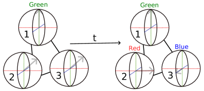
The QdLQA approach is inspired by local quantum annealing bowles_22 , and our goal is to start at the known minimum of one function and simulate a "quantum adiabatic evolution" into the minimum of a cost function for which the solution solves the optimization problem. During the quantum adiabatic evolution, we require that the system remains in a product state. At the end of the simulation, each local state is assigned a color, and Eq. (1) is used to calculate the energy. The scheme is illustrated in Fig. 1.
To simplify notation, we define the local probability vector , where each component (denoted by ) has a clear physical interpretation, namely they give the probability of measuring the -th eigenvalue of . This means that summing over all components for node gives . At each step in the quantum adiabatic evolution, a color configuration is generated by assigning each qudit to the state (color) corresponding to maximum probability .
We choose the initial cost function to be
| (8) |
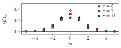
where indicates the dependence on all the angles in , , and initialize each qudit as the ground state of (which is a super position of different colors). The initial distribution is shown in Fig. 2. We note that the sum in Eq. (8) goes over all qudits except , which is the one with the most edges. This qudit is initialized with one color, e.g. , and is left untouched during the adiabatic evolution. The ability to do this is due to the invariance of any solution when swapping the labels of the colors, as such, we are free to choose the color for one single spin (the one with the most edges to simplify as much as possible).
For our final cost function, we choose the scalar product between probability vectors connected by the edges. This choice arises naturally from our ansatz since two orthogonal correspond to different colors. Using instead gives the components the interpretation of a measurement probability and emits antiferromagnetic (anti-parallel) solutions:
| (9) |
where , and are drawn from the uniform distribution in the interval at each time step during the quantum adiabatic evolution. We note that a similar cost function is used the in graph neural network approaches schuetz_22_2 ; wang_23 . There, however, the ’s emerge from applying the softmax function to the final node embedding. Note that contrary to the algorithm of bowles_22 , this cost function does not have an interpretation as the expectation value of a physical Hamiltonian on the considered quantum product states. Alternatively, we could also have formulated a cost function corresponding to Eq. (1) as a physical Hamiltonian in terms of polynomials in and deller_23 .
Furthermore, we follow Ref. wang_23 and introduce a term to force the qudits into superpositions of all the colors
| (10) |
where is a hyper parameter and the logarithm is taken component wise. For a large . this term favors a finite probability for all possible colors, even those that are initialized close to zero in the ground state of Fig. 2.
Finally, we conduct a quantum adiabatic evolution so that the total cost function becomes
| (11) |
In the simulation, we go from to using time steps. At each point in time, we conduct gradient descent steps ( indicates that we round to the nearest integer and is a hyper parameter). For some of the datasets discussed in Sec. III, we also find it beneficial to not start in the exact ground state of , but rather to start in states where we perturb the initial angles in Eq. (6) to , where are randomly chosen from the uniform distributed in the interval , and is a hyperparameter. Furthermore, we generate the classical color configuration at each time step and store the one with the lowest value for [see Eq. (1)], which provides the best configuration found by the algorithm.
For the alternate method focusing entirely on gradient descent, QdGD, each qudit is initialized in a random state with each qudit entry drawn from the uniform distribution in the interval . The state is then normalized, and is minimized directly by gradient descent. In this case, the are drawn at each gradient descent step and now the total number of steps is given by . We also introduce a further hyperparameter, Patience, which stops the algorithm early if no improvement in , Eq. (1), is seen after a certain number gradient descent steps.
In both cases, we sample over runs of the algorithm and each run is stopped if is found. We consider the best-found solutions and their frequency as indicators of the performance of the two algorithms.
To perform the gradient descent, we use the Adam optimizer kingma_14 with learning , specifically the PyTorch implementation paszke2019pytorch . All other parameters in the Adam optimizer were set to their PyTorch default values. A detailed list and description of all hyperparameters specific to the algorithms are provided in Appendix A.
III Benchmark
We benchmark our algorithms by considering several standard GCP instances used to test other methods hebrard_19 ; li_22 ; schuetz_22_2 ; wang_23 ; brighen_23 and comparing to results in the literature hebrard_19 ; schuetz_22_2 ; wang_23 . First, we consider Myciel and Queen graphs from the COLOR data set colordataset_02 and the citation networks Cora and Pubmed McCallum_2000 ; Sen_2008 ; nr-aaai15 . The Myciel and Queen graphs, based on Mycielski transformation and chessboards respectively, have up to 169 nodes and densities between and . In contrast, the Cora and Pubmed graphs have 2708 and 19717 nodes and densities of and . Note that a more thorough description of the datasets can be found in Ref. schuetz_22_2 .
We then consider three graphs from the SNAP library snapnets : The Facebook dataset based on social circles from Facebook, the Wikipedia vote dataset based on Wikipedia voting data, and the email-Eu-core data set based on Email communication between members of a research institute. For these three graphs, it is known hebrard_19 that relatively large numbers of colors are required to solve the problems (we use 70, 22, and 19) and thus they provide interesting challenges for our algorithms. In all cases, we consider undirected graphs, and we remove duplicated edges and any non-connected nodes when prepossessing the data.
III.1 Influence of the hyperparameters
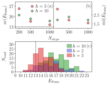
First, we illustrate how some of the hyperparameters in the QdLQA algorithm influence the final solutions. As an example, we show results for the queen11-11 graph. In Fig. 3(a), we demonstrate how the average value of the Potts energy depends on the number of time steps, , for different values of [which generates randomness in in Eq. (9)]. Increasing the number of steps improves the average quality of the solutions. The black dashed line shows the best value for reported in Ref wang_23 . Similar behaviour is seen for the standard deviation of the data in Fig. 3(b). Additionally, we see that for large , the data has a larger standard deviation and average value than . We observe that having a finite helps the algorithm escape from local minima, but if is chosen too large, this comes at the cost of more low-quality solutions. This is further illustrated in Fig. 3(c), where we show a histogram of the number of times, , a configuration with a certain energy is found. Again, the black dashed line shows the best value for reported in Ref wang_23 . There, we see how also choosing increases the fluctuations and leads to the algorithm getting stuck more frequently in a bad local minima. In 42 instances, the solution found by was out of the scale of the figure. Correspondingly, the data are also not plotted in Fig. 3(a).
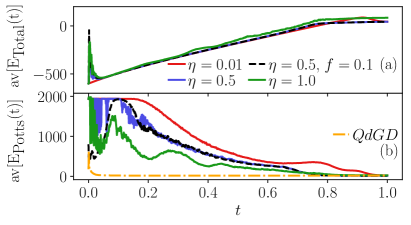
We now show an example of how the cost function and the Potts energy behave during the quantum adiabatic evolution in QdLQA. In Fig. 4, we plot both for the queen11-11 graph as a function of averaged over runs for different learning rates . For [Fig. 4(a)], we see that a large learning rate leads to an initial jump in the cost function, which increases when is increased. We attribute this jump to the fact that we start in the global minima at , which remains close to the minima for small increments in . Thus, doing a gradient descent step with a large learning rate will make us "overshoot" and take us away from the presumptive minima. However, we see that the curve quickly relaxes to the , whereas the curve also shows large fluctuations for later times. Note that in contrast to most schemes using the Adam optimizer, here, it depends on the energy landscape at previous times and the varying cost function [due to the randomness introduced by in Eq. (9)]. By setting (black dashed line), we observe that the amplitude of the initial jump increases, but that the curve soon follows the curve.
Figure 4(b) shows for the same parameters as Fig. 4(a). Here, one can see large fluctuations in the energies for and , but which decrease when is increased. The initial decay coincide with the jump in Fig. 4(a) and can be understood as follows: In the initial state, all qudits are initialized equally, and thus, has maximum value. If one now goes away from the minimum, this leads to different qudits taking on different colors, and thus the value of the final cost function will decrease. This can also be seen by changing the perturbation of the initial state (setting is illustrated by the black dashed line). Now, the qudit states on different nodes differ, and thus is smaller at . The orange curve in Fig. 4(b) shows for the QdGD algorithm (as a function of gradient descent steps ). Notably, this decays rapidly, which allows for a good solution to be found much earlier. When stopping the QdGD after having 100 gradient descent steps without improving , the average number of steps was (corresponding to ).
III.2 Comparing with other methods
| Graph | Nodes | Edges | colors (c) | Tabucol | PI-CGN | PI-SAGE | GNN-1N | ||||
| myciel5 | 47 | 236 | 6 | 0 | 0 | 0 | 0 | 0 | 0 | 100/100 | 100/100 |
| myciel6 | 95 | 755 | 7 | 0 | 0 | 0 | 0 | 0 | 0 | 38/100 | 97/100 |
| queen5-5 | 25 | 160 | 5 | 0 | 0 | 0 | 0 | 0 | 0 | 100/100 | 68/100 |
| queen6-6 | 36 | 290 | 7 | 0 | 1 | 0 | 0 | 0 | 0 | 12/100 | 7/100 |
| queen7-7 | 49 | 476 | 7 | 0 | 8 | 0 | 0 | 0 | 0 | 17/100 | 8/100 |
| queen8-8 | 64 | 728 | 9 | 0 | 6 | 1 | 1 | 0 | 0 | 6/100 | 2/100 |
| queen9-9 | 81 | 1056 | 10 | 0 | 13 | 1 | 1 | 0 | 0 | 3/100 | 1/100 |
| queen8-12 | 98 | 1368 | 12 | 0 | 10 | 0 | 0 | 0 | 0 | 27/100 | 41/100 |
| queen11-11 | 121 | 1980 | 11 | 20 | 37 | 17 | 13 | 10 | 13 | 1/100 | 2/100 |
| queen13-13 | 169 | 3328 | 13 | 25 | 61 | 26 | 15 | 12 | 15 | 2/100 | 1/100 |
| Cora | 2708 | 5429 | 5 | 0 | 1 | 0 | X | 1 | 0 | 3/100 | 1/100 |
| Pubmed | 19717 | 44338 | 8 | NA | 13 | 17 | X | 15 | 27 | 3/100 | 3/100 |
We now compare the solutions found by our algorithms to previously published results using graph neural networks in Refs. schuetz_22_2 ; wang_23 . In Table 1, we show the energies of the best configurations found with QdLQA and QdGD ( and respectively) and the fraction of the runs that found that energy ( and ) for different graphs. Furthermore, we show the corresponding values reported in Refs. schuetz_22_2 ; wang_23 obtained using a Tabucol hertz_87 and a greedy algorithm, a physics-inspired graph neural network solver (PI-SAGE) schuetz_22_2 , and graph neural networks using a first-order negative message passing strategy (GNN-1N) wang_23 . Note that if , the graph was colored with no conflicts, else, gives the remaining number of color clashes. For all the graphs except queen11-11, queen13-13, Cora, and PubMed, both our algorithms find the optimal solution. however, some graphs seem to be particularly hard. For example, for the queen8-8 and queen9-9 graphs, both algorithms only find the optimal solutions in of the 100 runs. For queen11-11 and queen13-13, QdLQA finds better solutions than those reported in Refs. schuetz_22_2 ; wang_23 . In the case of queen11-11, it additionally finds in three of the 100 runs, and both and in nine of the 100 runs each. For queen13-13, it additionally finds in two, in two, and in seven of the 100 runs.
By systematically increasing the number of colors used, we can get upper bounds for the chromatic number which we compare to those reported in Ref. schuetz_22_2 . For queen11-11, both our algorithms find with and (14 is found by the PI-SAGE algorithm in Ref. schuetz_22_2 , 11 is optimal) and queen13-13, both find with and (17 is found by the PI-SAGE algorithm in Ref. schuetz_22_2 , 13 is optimal).
For the Cora graph, only the QdGD algorithm finds the solution, and only in one of the 100 runs. QdLQA finds configurations in three and in 20 of the 100 runs, but requires a comparably large to do so (we use ). In this case, one must compromise between finding a few times at the cost of obtaining many bad solutions. For example, using instead, we get in 58 of 100 runs, but never . We also note that, as shown in Appendix A, the average runtime for one QdGD run on a laptop is significantly less than what is reported for PI-GCN in Ref. schuetz_22_2 for the same graphs on p3.2×large AWS EC2 instances.
For the PubMed graph, neither algorithm finds better solutions than the best one reported in Ref. schuetz_22_2 , but QdLQA seems to do significantly better than QdGD. Additionally, in contrast to the other datasets in Table 1, we do not fix the node with the largest number of edges for the PubMed graph. Rather, we fix a node with one edge as this improves the results. For , QdLQA improves from finding three times to finding and three, one, and seven times respectively. QdGD improves from finding twice to finding three times. This indicates that cleverly fixing one (or more) nodes might lead to further improvements.
III.3 Benchmarking using large number of colors
Finally, we test our algorithms on graphs where it is known that relatively large numbers of colors are needed to solve the problems hebrard_19 . In Table 2, we show results for the previously mentioned email-Eu-core, Facebook, and Wiki-vote datasets together with the corresponding upper and lower bounds provided in Ref. hebrard_19 (the problem was solved for email-Eu-core and Facebook). In our simulations, we use the number of colors equal to the upper bounds provided in Ref. brighen_23 (19 for email-Eu-core, 70 for Facebook, and 22 for Wiki-vote), and again, and give the number of conflicts in the best solution found. Even though neither algorithm solves the problem completely, they are clearly capable of providing relatively good solutions (quantified by the normalized error defined as the energy divided by number of edges, schuetz_22_2 ). For the email-Eu-core, Facebook, and Wiki-vote datasets, (0.0019), 0.00028 (0.00025) and 0.0019 (0.002) for QdLQA (QdGS). This demonstrates the ability of the algorithms to find good solutions for relatively large graphs requiring many colors on a simple laptop or desktop (see Appendix A for details).
| Graph | Nodes | Edges | ||||||
|---|---|---|---|---|---|---|---|---|
| email-Eu-core | 986 | 16064 | 19 | 19 | 26 | 30 | 1/100 | 1/100 |
| 4039 | 88234 | 70 | 70 | 25 | 22 | 1/100 | 1/100 | |
| Wiki-vote | 7115 | 103689 | 19 | 22 | 192 | 207 | 1/100 | 1/100 |
IV Conclusion
In this work, we have proposed two quantum-inspired algorithms to efficiently solve integer optimization problems. In our approach, we map nodes to qudits parameterized by -dimensional spherical coordinates and perform either local quantum annealing (QdLQA) or a gradient descent (QdGD).
We compared our results for a range of GCPs to some of the state-of-the-art methods in the literature schuetz_22_2 ; wang_23 , and both QdLQA and QdGD find equally good or better solutions for all of the test cases, with the exception of the Pubmed graph. We also tested the algorithms on graphs with large chromatic numbers hebrard_19 . Even though neither algorithm solved these problems completely, they still provided reasonable quality solutions (with normalized error ) using modest computing resources such as a desktop or a laptop. Notably, QdLQA almost always provided equally good or better solutions than QdGD (with the exception of the Cora and the Facebook graph). However, QdGD was heuristically found to be more efficient, since it minimizes the desired cost function directly. We refer the reader to Appendix A for further details.
There are many compelling possible extensions to our work. For example, each local Hilbert space dimension can be set manually, and thus, the approach can easily be extended to integer optimization problems requiring different numbers of states on each node. Furthermore, the interpretation of a vector on a sphere might provide new insights into why certain solutions are preferred (which can also be done with an analysis of the solutions and the interactions due to ). Additionally, there is also plenty of room for general optimizations, hyperparameter tuning, and different choices of, e.g., initial configurations. It will also be important to investigate if the algorithms can provide competitive solutions to GCPs containing millions of nodes, and see if they can be generalized to other problems, like large-scale graph-based machine learning tasks zheng2020distdgl ; hu2020open .
Acknowledgment
We acknowledge useful discussions with Márcio M. Taddei and Benjamin Schiffer and the support from the Government of Spain (European Union NextGenerationEU PRTR-C17.I1, Quantum in Spain, Severo Ochoa CEX2019-000910-S and FUNQIP), Fundació Cellex, Fundació Mir-Puig, the EU (NEQST 101080086, Quantera Veriqtas, PASQuanS2.1 101113690), the ERC AdG CERQUTE, the AXA Chair in Quantum Information Science and Generalitat de Catalunya (CERCA program). This project has received funding from the European Union’s Horizon 2020 research and innovation programme under the Marie Skłodowska-Curie grant agreement No 847517.
Appendix A Computer architectures and runtimes
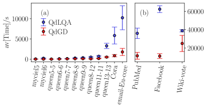
All computations, except those on the PubMed, Facebook, and Wiki-vote graphs, were run on a laptop with an 11th Gen Intel(R) Core(TM) i5-1135G7 @ 2.40GHz processor, whereas the latter ran on a desktop with an 11th Gen Intel(R) Core(TM) i5-11500 @ 2.70GHz processor. In Fig. 5, we plot the average computation time for one run for the different graphs for the parameters used in this work, see Appendix B. Note that parameters like and vary, so the figure is an illustration of the cost of obtaining the presented data, rather than fairly comparing the computational cost for the different graphs. Figure 5(a) shows the average time for one run of the algorithms for the different graphs on the laptop and Figure 5(b) on a stationary computer 111The partially large variances for QdLQA (and possibly for QdGD) comes from the fact that other processes were run simultaneously to the algorithms on the corresponding hardware.. As expected, the run time is significantly impacted by the Patience hyperparameter for QdGD, which allows the algorithm to stop early.
Appendix B Hyperparamters
There are several hyperparameters needed in both the QdLQA and the QdGD algorithms. These and their effects are summarized in Table 3. Additionally, the Adam optimizer has further hyperparameters that could be tuned (here, we only adjust the learning rate), however, in this work, they are left to their default values in PyTorch.
In Table 4, we show the hyperparameters used to produce the data in the Tables 1 and 2. In most cases, we found our default values , , and work well, however, for some graphs, we either started with the default values and tuned them manually or did a grid search. Note that for QdGD for the queen13-13 graph was chosen such that we get equally many gradient descent steps as in QdLQA with and .
| Hyperparameter | Algorithm | Description: |
| QdLQA | Number of steps used when going from to in the quantum adiabatic evolution. | |
| QdGD | Number of gradient descent steps. | |
| Both | Prefactor in from Eq. (10). | |
| QdLQA | Determines the number of gradient descent steps at each time step as . | |
| Both | Learning rate in the Adam optimizer. | |
| QdLQA | Determines the perturbation in the angles in the initial state. | |
| Both | Determines the perturbation in the interactions in the Potts model, see Eq. (9). | |
| Both | Number of times we run the algorithm. | |
| Patience | QdGD | If no improvement in is seen after this many gradient descent steps, the algorithm stops. |
| QdGD | Determines the sampling interval for each qudit in the intial state. |
| QdLQA | |||||||
|---|---|---|---|---|---|---|---|
| Graph | |||||||
| myciel5 | 1000 | 1.0 | 0.0 | 0.5 | 0.0 | 3.0 | 100 |
| myciel6 | 1000 | 1.0 | 0.0 | 0.5 | 0.0 | 3.0 | 100 |
| queen5-5 | 1000 | 1.0 | 0.0 | 0.5 | 0.0 | 3.0 | 100 |
| queen6-6 | 1000 | 1.0 | 0.0 | 0.5 | 0.0 | 3.0 | 100 |
| queen7-7 | 1000 | 1.0 | 0.0 | 0.5 | 0.0 | 3.0 | 100 |
| queen8-8 | 1000 | 1.0 | 0.0 | 0.5 | 0.1 | 3.0 | 100 |
| queen9-9 | 1000 | 1.0 | 0.0 | 0.5 | 0.0 | 3.0 | 100 |
| queen8-12 | 1000 | 1.0 | 0.0 | 0.5 | 0.0 | 3.0 | 100 |
| queen11-11 | 1000 | 1.0 | 0.0 | 0.5 | 0.1 | 3.0 | 100 |
| queen13-13 | 1000 | 0.75 | 2.0 | 0.5 | 0.0 | 3.0 | 100 |
| Cora | 1000 | 0.25 | 0.0 | 0.5 | 0.1 | 10.0 | 100 |
| Pubmed | 1000 | 0.1 | 0.0 | 0.1 | 0.5 | 3.0 | 100 |
| email-Eu-core | 1500 | 0.5 | 0.0 | 0.1 | 0.1 | 3.0 | 100 |
| 1000 | 0.1 | 0.0 | 0.1 | 0.1 | 3.0 | 100 | |
| Wiki-vote | 1000 | 0.1 | 0.0 | 0.5 | 0.1 | 3.0 | 100 |
| QdGD | ||||||
|---|---|---|---|---|---|---|
| Patience | ||||||
| 1000 | 1.0 | 100 | 0.5 | 1.0 | 3.0 | 100 |
| 1000 | 1.0 | 100 | 0.5 | 1.0 | 3.0 | 100 |
| 1000 | 1.0 | 100 | 0.5 | 1.0 | 3.0 | 100 |
| 1000 | 1.0 | 100 | 0.5 | 1.0 | 3.0 | 100 |
| 1000 | 1.0 | 100 | 1.0 | 1.0 | 1.0 | 100 |
| 1000 | 0.5 | 100 | 1.0 | 1.0 | 1.0 | 100 |
| 1000 | 0.5 | 100 | 0.1 | 1.0 | 1.0 | 100 |
| 1000 | 1.0 | 100 | 0.5 | 1.0 | 3.0 | 100 |
| 1000 | 1.0 | 100 | 0.5 | 1.0 | 3.0 | 100 |
| 3175 | 1.0 | 100 | 0.1 | 1.0 | 3.0 | 100 |
| 1000 | 0.5 | 100 | 1.0 | 1.0 | 3.0 | 100 |
| 1000 | 0.5 | 100 | 0.5 | 1.0 | 3.0 | 100 |
| 1000 | 0.5 | 100 | 0.1 | 1.0 | 1.0 | 100 |
| 1000 | 0.1 | 100 | 0.1 | 1.0 | 3.0 | 100 |
| 1000 | 0.1 | 100 | 0.5 | 1.0 | 3.0 | 100 |
References
- (1) J. Kallrath, Solving planning and design problems in the process industry using mixed integer and global optimization, Ann. Oper. Res. 140, 339 (2005).
- (2) W.-Y. Ku and J. C. Beck, Mixed integer programming models for job shop scheduling: A computational analysis, Comput. Oper. Res. 73, 165 (2016).
- (3) F. He and R. Qu, A two-stage stochastic mixed-integer program modelling and hybrid solution approach to portfolio selection problems, Inf. Sci. 289, 190 (2014).
- (4) R. M. R. Lewis, A Guide to Graph Colouring: Algorithms and Applications (Springer, Heidelberg, 2016).
- (5) M. Garey, D. Johnson, and L. Stockmeyer, Some simplified NP-complete graph problems, Theor. Comput. Sci. 1, 237 (1976).
- (6) N. Barnier and P. Brisset, Graph coloring for air traffic flow management, Ann. Oper. Res. 130, 163 (2004).
- (7) Y. Deller, S. Schmitt, M. Lewenstein, S. Lenk, M. Federer, F. Jendrzejewski, P. Hauke, and V. Kasper, Quantum approximate optimization algorithm for qudit systems, Phys. Rev. A 107, 062410 (2023).
- (8) E. Farhi, J. Goldstone, and S. Gutmann, A quantum approximate optimization algorithm, arXiv:1411.4028 (2014).
- (9) S. Hadfield, Z. Wang, B. O’Gorman, E. G. Rieffel, D. Venturelli, and R. Biswas, From the quantum approximate optimization algorithm to a quantum alternating operator ansatz, Algorithms 12 (2019).
- (10) Y.-H. Oh, H. Mohammadbagherpoor, P. Dreher, A. Singh, X. Yu, and A. J. Rindos, Solving multi-coloring combinatorial optimization problems using hybrid quantum algorithms, arXiv:1911.00595 (2019).
- (11) P. Hauke, H. G. Katzgraber, W. Lechner, H. Nishimori, and W. D. Oliver, Perspectives of quantum annealing: methods and implementations, Rep. Prog. Phys. 83, 054401 (2020).
- (12) B. Pokharel, Z. Gonzalez Izquierdo, P. A. Lott, E. Strbac, K. Osiewalski, E. Papathanasiou, A. Kondratyev, D. Venturelli, and E. Rieffel, Inter-generational comparison of quantum annealers in solving hard scheduling problems, arXiv:2112.00727 (2021).
- (13) S. Yarkoni, E. Raponi, T. Bäck, and S. Schmitt, Quantum annealing for industry applications: introduction and review, Rep. Prog. Phys. 85, 104001 (2022).
- (14) A. Lucas, Ising formulations of many NP problems, Front. Phys. 2 (2014).
- (15) F. Glover, G. Kochenberger, R. Hennig, and Y. Du, Quantum bridge analytics I: a tutorial on formulating and using QUBO models, Ann. Oper. Res. 314, 141 (2022).
- (16) H.-H. Lu, Z. Hu, M. S. Alshaykh, A. J. Moore, Y. Wang, P. Imany, A. M. Weiner, and S. Kais, Quantum phase estimation with time-frequency qudits in a single photon, Adv. Quantum Technol. 3, 1900074 (2020).
- (17) Y. Wang, Z. Hu, B. C. Sanders, and S. Kais, Qudits and high-dimensional quantum computing, Front. Phys. 8 (2020).
- (18) M. Ringbauer, M. Meth, L. Postler, R. Stricker, R. Blatt, P. Schindler, and T. Monz, A universal qudit quantum processor with trapped ions, Nat. Phys. 18, 1053 (2022).
- (19) G. Bottrill, M. Pandey, and O. Di Matteo, Exploring the potential of qutrits for quantum optimization of graph coloring, 2023 IEEE International Conference on Quantum Computing and Engineering (QCE), volume 01, 177–183 (2023).
- (20) J. A. Smolin and G. Smith, Classical signature of quantum annealing, Front. Phys. 2 (2014).
- (21) M. T. Veszeli and G. Vattay, Mean field approximation for solving QUBO problems, PLOS ONE 17, 1 (2022).
- (22) J. Bowles, A. Dauphin, P. Huembeli, J. Martinez, and A. Acín, Quadratic unconstrained binary optimization via quantum-inspired annealing, Phys. Rev. Appl. 18, 034016 (2022).
- (23) B. Bauer, L. Wang, I. Pižorn, and M. Troyer, Entanglement as a resource in adiabatic quantum optimization, arXiv:1501.06914 (2015).
- (24) S. Mugel, C. Kuchkovsky, E. Sánchez, S. Fernández-Lorenzo, J. Luis-Hita, E. Lizaso, and R. Orús, Dynamic portfolio optimization with real datasets using quantum processors and quantum-inspired tensor networks, Phys. Rev. Res. 4, 013006 (2022).
- (25) J. Gomes, K. A. McKiernan, P. Eastman, and V. S. Pande, Classical quantum optimization with neural network quantum states, arXiv:1910.10675v1 (2019).
- (26) T. Zhao, G. Carleo, J. Stokes, and S. Veerapaneni, Natural evolution strategies and variational Monte Carlo, Mach. Learn.: Sci. Technol. 2, 02LT01 (2020).
- (27) M. J. A. Schuetz, J. K. Brubaker, and H. G. Katzgraber, Combinatorial optimization with physics-inspired graph neural networks, Nat. Mach. Intell. 4, 367–377 (2022).
- (28) S. A. Khandoker, J. M. Abedin, and M. Hibat-Allah, Supplementing recurrent neural networks with annealing to solve combinatorial optimization problems, Mach. Learn.: Sci. Technol. 4, 015026 (2023).
- (29) E. S. Tiunov, A. E. Ulanov, and A. I. Lvovsky, Annealing by simulating the coherent Ising machine, Opt. Express 27, 10288 (2019).
- (30) H. Goto, K. Tatsumura, and A. R. Dixon, Combinatorial optimization by simulating adiabatic bifurcations in nonlinear Hamiltonian systems, Sci. Adv. 5, eaav2372 (2019).
- (31) H. Goto, K. Endo, M. Suzuki, Y. Sakai, T. Kanao, Y. Hamakawa, R. Hidaka, M. Yamasaki, and K. Tatsumura, High-performance combinatorial optimization based on classical mechanics, Sci. Adv. 7, eabe7953 (2021).
- (32) E. Hebrard and G. Katsirelos, A hybrid approach for exact coloring of massive graphs, Integration of Constraint Programming, Artificial Intelligence, and Operations Research, edited by L.-M. Rousseau and K. Stergiou, 374–390 (Springer International Publishing, Cham, 2019).
- (33) M. J. A. Schuetz, J. K. Brubaker, Z. Zhu, and H. G. Katzgraber, Graph coloring with physics-inspired graph neural networks, Phys. Rev. Res. 4, 043131 (2022).
- (34) X. Wang, X. Yan, and Y. Jin, A graph neural network with negative message passing and uniformity maximization for graph coloring, Complex Intell. Syst. 10, 4445 (2024).
- (35) R. B. Potts, Some generalized order-disorder transformations, Math. Proc. Camb. Philos. Soc. 48, 106–109 (1952).
- (36) F. Y. Wu, The Potts model, Rev. Mod. Phys. 54, 235 (1982).
- (37) F. Y. Wu, Potts model and graph theory, J. Stat. Phys. 52, 99 (1988).
- (38) L. Zdeborová and F. Krząkała, Phase transitions in the coloring of random graphs, Phys. Rev. E 76, 031131 (2007).
- (39) D. P. Kingma and J. Ba, Adam: A method for stochastic optimization, arXiv:1412.6980 (2014).
- (40) A. Paszke, S. Gross, F. Massa, A. Lerer, J. Bradbury, G. Chanan, T. Killeen, Z. Lin, N. Gimelshein, L. Antiga, A. Desmaison, A. Köpf, E. Yang, Z. DeVito, M. Raison, A. Tejani, S. Chilamkurthy, B. Steiner, L. Fang, J. Bai, and S. Chintala, PyTorch: An Imperative Style, High-Performance Deep Learning Library, Proceedings of the 33rd International Conference on Neural Information Processing Systems (Curran Associates Inc., Red Hook, NY, USA, 2019).
- (41) W. Li, R. Li, Y. Ma, S. On Chan, D. Pan, and B. Yu, Rethinking graph neural networks for the graph coloring problem, arXiv:2208.06975 (2022).
- (42) A. Brighen, H. Slimani, A. Rezgui, and H. Kheddouci, A new distributed graph coloring algorithm for large graphs, Clust. Comput. (2023).
- (43) M. Trick, COLOR dataset, URL (accessed Dec. 2023), https://mat.tepper. cmu.edu/COLOR02/ (2002).
- (44) A. K. McCallum, K. Nigam, J. Rennie, and K. Seymore, Automating the construction of internet portals with machine learning, Information Retrieval 3, 127 (2000).
- (45) P. Sen, G. Namata, M. Bilgic, L. Getoor, B. Galligher, and T. Eliassi-Rad, Collective classification in network data, AI Magazine 29, 93 (2008).
- (46) R. A. Rossi and N. K. Ahmed, The network data repository with interactive graph analytics and visualization, AAAI (2015).
- (47) J. Leskovec and A. Krevl, SNAP Datasets: Stanford large network dataset collection, http://snap.stanford.edu/data (2014).
- (48) A. Hertz and D. de Werra, Using tabu search techniques for graph colorin, Computing 39, 345–351 (1987).
- (49) D. Zheng, C. Ma, M. Wang, J. Zhou, Q. Su, X. Song, Q. Gan, Z. Zhang, and G. Karypis, Distdgl: distributed graph neural network training for billion-scale graphs, 2020 IEEE/ACM 10th Workshop on Irregular Applications: Architectures and Algorithms (IA3), 36–44 (IEEE, 2020).
- (50) W. Hu, M. Fey, M. Zitnik, Y. Dong, H. Ren, B. Liu, M. Catasta, and J. Leskovec, Open graph benchmark: Datasets for machine learning on graphs, Advances in neural information processing systems 33, 22118 (2020).
- (51) The partially large variances for QdLQA (and possibly for QdGD) comes from the fact that other processes were run simultaneously to the algorithms on the corresponding hardware.