fff Rotating reduced Kiselev black holes:
Shadows, Energy emission and Deflection of light

Abstract

In this paper, we generate a rotating solution of the reduced Kiselev black hole through the modified Newman-Janis formalism. Based on such solution, we remark different shadow behaviors by varying the involved parameters $r_{k},a,\alpha$. Concretely, we observe that the allowed values of the spin parameter $a$ are much less than the usual rotating black holes. By deeply analysing the shadow shapes, we show that comparable shadow shapes emerge for the same ratio $a/r_{k}$. On the other hand, we recognize that the parameters $a$ and $\alpha$ governs the shadow geometry while the parameter $r_{k}$ rules the size of such a quantity. Besides, we notice that an elliptic shadow geometry appears for certain range of relevant parameters. By making contact with the observational side, we provide a constraint on the rotating reduced Kiselev (RRK) black hole parameters. In particular, we find a good compatibility between the theoretical and experimental results. Regarding Hawking radiation, we note that the Kiselev radius $r_{k}$ shows a similar behavior to the quintessence filed intensity $\mathbf{c}$. Concerning the light motion in the vicinity of a RRK black hole, we investigate deeply the deflection by varying the relevant parameters. In particular, we remark that such a quantity decreases by increasing the parameters $a$ and $\alpha$ while the opposite effect is observed when increasing $r_{k}$.

Keywords: Black holes, Shadow, Deflection angle, Dark Energy.

1 Introduction

Due to its intriguing and challenging aspects, physicists have been particularly interested in black holes for a long time. The carried researches have been considered as a crucial chance to widen our knowledge of the basic principles of physics with a special interest towards general relativity and quantum mechanics. In the study of black holes, vital explanations about the nature of the univers emerge. Thus, many inspections have been conducted to explain the enigmatic phenomena in the heart of black hole physics. In addition, the existence of these mysterious objects was recently proven through images captured by the Event Horizon Telescope (EHT) [1, 2, 3]. Moreover, it have been considered as a significant achievement of Einstein’s gravitation theory [4]. These images gave an unprecedented opportunity for scientists around the world to explore the details of these cosmic objects[5, 6, 7, 8, 9, 10, 11, 12, 13, 14, 15, 16, 17, 18, 19].

Many areas of black hole physics can be examined. Essentially, the shadow of the black hole can constrain the alternative gravitational theories and is especially rich in information on the mechanics of such celestial objects [20]. Additionally, black holes deflect light because of their strong gravitational attraction, which offers a special perspective for research on these enormous cosmic objects. With the use of such aspect, scientists can explore the gravitational environment of this object and test Einstein’s theory [21, 22, 23, 24, 25, 26, 27, 28, 29, 30, 33, 34, 31, 32]. As a result, the optical along with the thermodynamic aspects of these objects have been the focus of numerous studies [35, 36, 37, 38, 39, 40, 41, 42, 43, 44, 45, 46, 47, 48, 49, 50, 51, 52, 53, 54, 57, 56, 55]. More specifically, by adopting a thermodynamic interpretation of the cosmological constant, an investigation of the optical and thermodynamical aspect of charged, rotating and non-rotating black holes was carried [58, 59, 60, 61]. Besides, such cosmological constant has been used in order to analyze the stability and phase transitions, observed in multiple types of black holes present in supergravity theories. These studies have been expended by considering the existence of a real scalar field modeling the dark energy and dark matter effects. Indeed, the latter, which makes up around 70% of the total matter in the universe, has been a favorite candidate to interpret the universe expansion. This form of energy exerts a negative pressure that promotes the cosmic expansion [62, 63, 64, 65, 66]. More precisely, the quintessential scalar field can be considered as a candidate to describe the dark energy. It is defined as a real, spatially homogeneous scalar field characterized by an intensity $\mathbf{c}$[67, 68]. In this context, an equation of state $p=\omega\rho$ constraint the pressure $p$ and the energy density $\rho$. In addition, the state parameter $\omega$ being the ratio of the pressure to the energy density describes different models depending on its value. This parameter could take a specific valus depending on the constraint $-1<\omega<-1/3$[69, 70, 71]. In this way, the state parameter $\omega$ being the ratio of the pressure to the energy density describes different models depending on its value. For instance, the state parameter $\omega=-1$ is assigned to the cosmological constant model while the case $-1/3<\omega<0$ can be associated to different models, i.e quintessence or K-essence [72, 73, 74].

Moreover, the quintessence field could be considered as a part of Kiselev solution [75]. In particular, various studies have been carried out on the optical and thermodynamical of Kiselev black holes [76, 77, 78, 79]. Looking more closely at the Kiselev model, one could consider a positive tangential pressure value in which the $r_{g}$ representing the mass term is set zero and $-1/3<\omega<0$ [80]. In this situation, the model is so-called reduced Kiselev black hole and the event horizon radius of this model exists at Kiselev radius $r_{k}$. This type of black hole is different from the Schwarzschild black hole, where such a difference has been explained by the existence of a gravitational potential.

In this work, the main aim is to advance in the area of black hole physics by exploring the physics behind the RRK case. Concretely, we inspect the optical characteristics of the RRK black holes by varying the parameters $r_{k},a,\alpha$. Particularly, we study the geometry by investigating the ergosphre and horizons regions. Then, we investigate the shadow while comparing our results to the Kerr and quintessential black holes. Indeed, the shadow graphs demonstrate that the RRK black hole can match precisely the Kerr solution. Eventually, the emission rate and the deflection of light are examined for various parameters defining the RRK black hole.

The paper is organized in the following structure. Section 2 is devoted to the determination of the rotating solution by using the Newman-Janis formalisme. In section 3, we explore the optical behaviors and energy aspects associated with the solution. Indeed, in 3.1 we construct the equations of motion and explain the different shadow aspects of the RRK solution according to the involved parameters. Then, we constrain the later by comparing our results to the observation data. After exploring the Hawking radiation in section 3.3, we investigate the deviation of light by the RRK solution. In this work, we use the units in which the light speed $c$, the reduced Planck constant $\hbar$ and Newton’s constant $G$ are set as $c=G=\hbar=1$.

2 Rotating solution of the reduced Kiselev black hole

In this section, we provide the rotating solution of the reduced Kiselev black hole using the Newman-Janis method without complexifcation for a general static and spherically symmetric metric. Such a procedure, was developped to avoid the complexification step known to provide a non-unique final solution [81, 82, 83]. We then present the necessary tensors and discuss the relevant geometric characteristics of the RRK solution.

2.1 Newman-Janis procedure without complexification

In order to determine the RRK solution, we consider the general case of the statical and spherically symmetrical space-time

$$ds_{RRK}^{2}=-F(r)dt^{2}+G(r)^{-1}dr^{2}+H(r)d\Omega_{s}^{2},$$ (2.1)

where $d\Omega_{s}^{2}=d\theta^{2}+\sin^{2}\theta d\phi^{2}$. First, with the use of the  Eddington-Finkelstein coordinates $\left(u,r,\theta,\phi\right)$, the metric could be transformed as follows

$$ds_{RRK}^{2}=-F(r)du^{2}-2\sqrt{\frac{F}{G}}dudr+H(r)d\Omega^{2},$$ (2.2)

where

$$dv=dt-\frac{dr}{\sqrt{F\,G}}.$$ (2.3)

In this way, the inverse metric and the tetrad vectors are expressed in terms of the null tetrad $Z_{\alpha}^{\mu}=(l^{\mu},n^{\mu},m^{\mu},\bar{m}^{\mu})$ as

$$g^{\mu\nu} = -l^{\mu}n^{\nu}-l^{\nu}n^{\mu}+m^{\mu}\bar{m}^{\nu}+m^{\nu}\bar{m}^{\mu},$$ (2.4)

$$l_{\mu}l^{\mu} = n_{\mu}n^{\mu}=m_{\mu}m^{\mu}=l_{\mu}m^{\mu}=n_{\mu}m^{\mu}=0.$$ (2.5)

Thus, we find the following tetrad vectors

$$l^{\mu}=\delta^{\mu}_{r},\hskip 5.69046ptn^{\mu}=\sqrt{\frac{G}{F}}\delta^{\mu}_{u}-\frac{G}{2}\delta^{\mu}_{r},\quad m^{\mu}=\frac{1}{\sqrt{2H}}\left(\delta^{\mu}_{\theta}+\frac{i}{\sin\theta}\delta^{\mu}_{\phi}\right).$$ (2.6)

Concretely, the associated vectors satisfy the following relation

$$l_{\mu}n^{\mu}=-m_{\mu}\bar{m}^{\mu}=-1.$$ (2.7)

Using the complex notation, we apply a mathematical transformation on the $r-u$ plane of the static metric, which results in a rotating black hole metric

$$r\rightarrow r^{\prime}=r+ia\cos\theta,\hskip 8.5359ptu\rightarrow u^{\prime}=u-ia\cos\theta.$$ (2.8)

The new tetrad vectors become

$$l^{\prime\mu} = \delta^{\mu}_{r},$$ (2.9)

$$n^{\prime\mu} = \sqrt{\frac{B(r,\theta)}{A(r,\theta)}}\delta^{\mu}_{u}-\frac{B(r,\theta)}{2}\delta^{\mu}_{r},$$ (2.10)

$$m^{\prime\mu} = \frac{1}{\sqrt{2C(r,\theta)}}\left(ia\sin\theta(\delta^{\mu}_{u}-\delta^{\mu}_{r})+\delta^{\mu}_{\theta}+\frac{i}{\sin\theta}\delta^{\mu}_{\phi}\right),$$ (2.11)

where the functions $\left\{F(r),G(r),H(r)\right\}$ are replaced by $\left\{A(r,\theta),B(r,\theta),C(r,\theta)\right\}$. A close examination reveals that the new metric in advanced null coordinates can be obtained using its inverse version. In fact, the revised metric is now given by

$$ds^{2} = -Adu^{2}-2\sqrt{\frac{A}{B}}dudr+2a\sin^{2}\theta\left(A-\sqrt{\frac{A}{B}}\right)dud\phi+2a\sqrt{\frac{A}{B}}\sin^{2}\theta drd\phi$$ (2.12)

$$+Cd\theta^{2}+\sin^{2}\theta\left[C+a^{2}\sin^{2}\theta\left(2\sqrt{\frac{A}{B}}-A\right)\right]d\phi^{2},$$

where

$$du=dt^{\prime}+\gamma(r)dr,\hskip 14.22636ptd\phi=d\phi^{\prime}+\beta(r)dr.$$ (2.13)

An analysis reveals that the complexification sequence of the Newman-Janis method could be solved by introducing new real functions[84, 81, 82, 83]. These functions satisfy to the following constraint

$$\lim_{a\to 0}D(r,\theta,a)=B(r),\hskip 8.5359pt\lim_{a\to 0}E(r,\theta,a)=A(r),\hskip 8.5359pt\lim_{a\to 0}\Psi(r,\theta,a)=C(r),$$ (2.14)

where

$$\gamma(r)=-\frac{(H\sqrt{F}+a^{2}\sqrt{G})}{\sqrt{G}(FH+a^{2})},\,\beta(r)=-\frac{a}{FH+a^{2}},$$ (2.15)

and

$$A(r,\theta)=\frac{\sqrt{G}(FH+a^{2}\cos^{2}\theta)\Psi}{(H\sqrt{F}+a^{2}\sqrt{G}\cos^{2}\theta)^{2}},\,B(r,\theta)=\frac{FH+a^{2}\cos^{2}\theta}{\Psi}.$$ (2.16)

In this setup, the function $\Psi(r,\theta,a)$ is still unknown. However, the explicit expression of this function could be determinate by using the following constraint

$$(I+a^{2}x^{2})^{2}(3\frac{\partial\Psi}{\partial r}\frac{\partial\Psi}{\partial x^{2}}-2\Psi\frac{\partial\Psi}{\partial(rx^{2})})=3a^{2}\frac{\partial I}{\partial r}\,\Psi^{2},$$ (2.17)

$$[(\frac{\partial I}{\partial r})^{2}+I(2-\frac{\partial^{2}I}{\partial r^{2}})-a^{2}x^{2}(2+\frac{\partial^{2}I}{\partial r^{2}})]\Psi$$

$$+(I+a^{2}x^{2})(4x^{2}\frac{\partial\Psi}{\partial x^{2}}-\frac{\partial I}{\partial r}\frac{\partial\Psi}{\partial r})=0,$$ (2.18)

where

$$I(r) \equiv H(r)\sqrt{\frac{F(r)}{G(r)}},$$ (2.19)

$$x = \cos\theta.$$ (2.20)

Concretely, Eq.(2.17) is obtained by imposing $G_{r,\theta}=0$ with $G_{r,\theta}$ being the tensor component of the Einstein equations. However, Eq.(2.18) is derived by the help of the filed equation $G_{\mu\nu}=T_{\mu\nu}$ (see the appendix of ref[81]). After the calculations, the associated function $\Psi$ is written as

$$\Psi=r^{2}+a^{2}\cos^{2}\theta.$$ (2.21)

Taking the expression of the involved functions $A$, $B$ and $\Psi$, the line element of the metric in the Boyer-Lindquist coordinates associated with RRK black hole is

$$ds^{2}=-(1-\frac{f}{\Psi})dt^{2}+\frac{\Psi}{\Delta_{RRK}}dr^{2}+\Psi d\theta^{2}+\frac{\Sigma\sin^{2}\theta}{\Psi}d\phi^{2}-\frac{2af\sin^{2}\theta}{\Psi}dtd\phi.$$ (2.22)

The reduced function terms associated with the solution are expressed as follows

$$f=\frac{r_{k}^{\alpha}}{r^{\alpha-2}},\hskip 8.5359pt\Delta_{RRK}=r^{2}+a^{2}-f,\hskip 8.5359pt\Sigma=(r^{2}+a^{2})^{2}-a^{2}\Delta_{RRK}\sin^{2}\theta,$$ (2.23)

At this point, $\alpha$ is linked to the state parameter $\omega$ by the following equation

$$\alpha=3\omega+1,$$ (2.24)

where $r_{k}$ being the Kiselev radius. In particular, for $\alpha=1$ and $r_{k}=2M$ we get the line element of Kerr black hole solution. In our investigation, we consider $0<\alpha<1$ which is associated to the range $-1/3<\omega<0$. In this case, the quintessence model behaves as quintessence energy while the case $-1<\omega<-1/3$ behaves as phantom energy. Since the new generated solution is completely different from the reduced-Kiselev black hole of the metric (2.1), the Einstein tensor still needs to be determined. It is noted that, the modified Newman-Janis procedure is a method used to transform a non-rotating solution to a rotating one. However, the obtained solution does not have the same tensors as the non-rotating case. As a result, we report in this part the Einstein tensor associated with the RRK black hole. Indeed, after computations and simplifications, it can be shown that the non vanishing Einstein tensor components are

$$G_{rr} =\frac{2(\alpha-1)r^{2}r_{k}^{\alpha}}{\left(a^{2}\cos(2\theta)+a^{2}+2r^{2}\right)\left(\left(a^{2}+r^{2}\right)r^{\alpha}-r^{2}r_{k}^{\alpha}\right)},$$ (2.25)

$$G_{\theta\theta} =-\frac{(\alpha-1)r^{-\alpha}r_{k}^{\alpha}\left(a^{2}(\alpha-2)\cos^{2}(\theta)+\alpha r^{2}\right)}{a^{2}\cos(2\theta)+a^{2}+2r^{2}},$$ (2.26)

$$G_{\phi t} =\frac{2a(\alpha-1)\sin^{2}(\theta)r^{-2\alpha}r_{k}^{\alpha}\left(\left(a^{2}+r^{2}\right)r^{\alpha}\left((\alpha-2)a^{2}\cos(2\theta)+(\alpha-2)a^{2}+2(\alpha+2)r^{2}\right)-4r^{4}r_{k}^{\alpha}\right)}{\left(a^{2}\cos(2\theta)+a^{2}+2r^{2}\right)^{3}},$$ (2.27)

$$=G_{t\phi},$$

$$G_{tt} =\frac{(\alpha-1)r_{k}^{\alpha}}{2r^{2\alpha}\left(a^{2}\cos(2\theta)+a^{2}+2r^{2}\right)^{3}}$$ (2.28)

$$\times\left[r^{\alpha}\left((\alpha-2)a^{4}\cos(4\theta)-(\alpha-2)a^{4}+4\alpha a^{2}r^{2}\cos(2\theta)-4(\alpha+4)a^{2}r^{2}-16r^{4}\right)+16r^{4}r_{k}^{\alpha}\right],$$

$$G_{\phi\phi} =-\frac{2(\alpha-1)\sin^{2}(\theta)r_{k}^{\alpha}}{r^{2\alpha}\left(a^{2}\cos(2\theta)+a^{2}+2r^{2}\right)^{3}}$$ (2.29)

$$\times\left[\left(a^{2}+r^{2}\right)r^{\alpha}\left((\alpha-2)a^{4}+a^{2}\cos(2\theta)\left((\alpha-2)a^{2}+(\alpha-4)r^{2}\right)+3\alpha a^{2}r^{2}+2\alpha r^{4}\right)\right.$$

$$\qquad\left.-4a^{2}r^{4}\sin^{2}(\theta)r_{k}^{\alpha}\right]$$

It must be clarified that the modified Newman-Janis procedure pemits the introduction of symmetry feature and more physical reasons in addition to avoiding the complexification process. Moreover, it has been remarked that such a modified method is effective in cases where the original Newman-Janis process has failed.

2.2 Horizon geometry and ergosphere

To inspect the RRK black hole geometry, it is useful to recall that the solution of $\Delta=0$ provides information about the horizon radius. For example, considering $\alpha=1$, we can easily determine the inner and outer horizons that are located at

$$r_{-}=\frac{1}{2}\left(r_{k}-\sqrt{r_{k}^{2}-4a^{2}}\right),\quad r_{+}=\frac{1}{2}\left(r_{k}+\sqrt{r_{k}^{2}-4a^{2}}\right).$$ (2.30)

It is clear from such equations that the Kerr black hole horizons are obtained by replacing $r_{k}=2M$. In the extremal case, the inner and outer horizon coincide $r_{-}=r_{+}$ and such a case is equivalent to setting $r_{k}=2a$. To study the aspects of the RRK black hole geometry, we illustrate in figure (1) the metric function $\Delta$ with respect to the radial coordinate $r$ for various values of the concerned parameters.

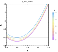
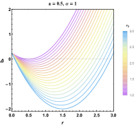
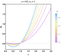
Figure 1: Delta metric function of RRK black hole for different values of the spin, Kiselev radius and $\alpha$ parameters.

From such a figure, it can be confirmed that the RRK black hole is characterized by an inner and outer horizon for most cases. The remaining ones are associated with the extremal case in which the inner and outer horizon coincide. For the left panel, we vary the rotation parameter $a$. Clearly, we observe for $r_{k}=1$ and $\alpha=1$ that the extremal case is reached for $a=0.5$ while for lowest values of such parameter the black hole exhibits two horizons. For the middle panel, it can be noticed that the gap between the inner and outer horizon increases with $r_{k}$. For the $\alpha$ effect, we see that the inner horizon gets smaller when such a parameter is increased while the outer horizon shows the opposite effect.
In order to fully explore the geometry of the RRK solution, we examine now the ergosphere region which is confined by the event horizon and a static limit surface. Such region is localized outside the black hole. In fact, the ergoregion correspond to the region where the Killing vector $\chi^{a}$ could be viewed as a space-like vector. An interesting phenomenon can occur in this particular region of space-time. In fact, a particle can remain stationary in the ergosphere and can exit the such region. For the present solution, the ergosphere region could be calculated by the help of this following equation

$$r^{2}+a^{2}\cos^{2}\theta-f=0$$ (2.31)

Using the polar coordinate, we illustrate in figure (5) the ergospheres region and the horizons for different values of the involved parameters . In particular, for $\theta=\pi$, the equation of ergospheres and the horizons are identical. From such a figure, we observe that the size of the plotted quantities increases with $r_{k}$. Besides, it can confirmed that the gap between the inner and outer horizon increases with $r_{k}$. In addition, we can see that the outer ergosphere becomes more stretched in by increasing $r_{k}$ or $a$ . Comparing the graphs, we remark by decreasing $\alpha$ that the ergosphere becomes more prolate.

Figure 2: Ergosphere region and the horizon variation for different values of the relevant parameters. The purple and orange colors are associated with the ergosphere region and the horizons, respectively.

In the next setup, we analyze the optical behavior of the present solution by varying the relevant parameters including $\alpha$ and $r_{k}$.

3 Shadow aspects of RRK black hole

In this section, we aim to study the optical aspect of RRK solution. Concretely, we investigate the shadow behaviors and energy emission rate in terms of the relevant parameters associated with the present solution. Moreover, we make contact with EHT observational data by deposing the constraint on such parameters and explore.

3.1 Shadow aspects of RRK black hole

In this part, we inspect the optical aspect of RRK black hole by exploiting the Hamilton-Jacobi method[85]. Indeed, this equation represents the motion of a particle in the associated space-time which is controlled by the Jacobi action $\mathcal{S}$. In particular, for a massless particle one can use

$$\frac{\partial\mathcal{S}}{\partial\lambda}=-\frac{1}{2}g^{\mu\nu}p_{\mu}p_{\nu},$$ (3.1)

where $p$ and $\lambda$ are the four-momentum quantities and the affine parameter, respectively. Concretely, the Jacobi action in the spherically symmetric space-time has the following form

$$\mathcal{S}=-Et+L\phi+S_{r}(r)+S_{\theta}(\theta),$$ (3.2)

where the conserved angular momentum $L=p_{\phi}$ and the conserved total energy $E=-p_{t}$ are associated with the four-momentum components of $p_{\mu}$. Besides, $S_{\theta}(\theta)$ and $S_{r}(r)$ depend respectively on the angular parameter $\theta$ and the radial coordinate $r$. Using the separation method, the null geodesic equations is derived by using the Carter mechanism [85]. For simplicity reason, we introduce two parameters defined in terms of the conserved angular momentum, the total energy and the separable constant $\mathcal{K}$

$$\xi_{RRK}=\frac{L}{E},\hskip 42.67912pt\eta_{RRK}=\frac{\mathcal{K}}{E^{2}}.$$ (3.3)

Using theses two quantities, the null geodesic equations of RRK black hole are derived by solving the following equations

$$\Psi\frac{d\,t}{d\tau} =E\left[\frac{r^{2}+a^{2}}{\Delta_{RRK}}\left(r^{2}+a^{2}-a\xi\right)+a\left(\xi-a\sin^{2}\theta\right)\right],$$ (3.4)

$$\Psi\frac{d\,r}{d\tau} =\sqrt{\mathcal{R}(r}),$$ (3.5)

$$\Psi\frac{d\,\theta}{d\tau} =\sqrt{\Theta(\theta)},$$ (3.6)

$$\Psi\frac{d\,\phi}{d\tau} =E\left[\frac{a}{\Delta_{RRK}}\left(r^{2}+a^{2}-a\xi\right)+\left(\frac{\xi}{\sin^{2}}-a\right)\right],$$ (3.7)

where the radial and the polar functions are expressed as follows

$$\mathcal{R}(r) =E^{2}\left[\left[\left(r^{2}+a^{2}\right)-a\xi_{RRK}\right]^{2}-\Delta_{RRK}(\eta+(\xi-a)^{2})\right],$$ (3.8)

$$\Theta(\theta) =E^{2}\left[\eta_{RRK}-\frac{1}{\sin^{2}\theta}\left(a\sin^{2}\theta-\xi_{RRK}\right)^{2}+(\xi-a)^{2}\right].$$ (3.9)

With the use of the radial function and the conditions bellow, we can elaborate the shadow of such model

$$\mathcal{R}(r)\Big{|}_{r=r_{0}}=\frac{d\mathcal{R}(r)}{dr}\Big{|}_{r=r_{0}}=0,$$ (3.10)

where, $r_{0}$ is the radius of photon sphere. Various equations are used to determine this radius for different black hole solutions[35, 36, 37, 38, 39, 40, 41, 42, 43, 44, 45, 46, 47, 48, 49, 50, 51, 52, 53, 55, 56]. Considering $\Theta(\theta)>0$, the parameters $\xi$ and $\eta$ are expressed as a function of the involved parameters associated with the RRK black hole solution. Indeed, we obtain

$$\eta_{RRK}=\frac{a^{2}\left((\alpha-2)r_{k}^{\alpha}-2r^{\alpha}\right)+r^{2}\left((\alpha+2)r_{k}^{\alpha}-2r^{\alpha}\right)}{a\left(2r^{\alpha}+(\alpha-2)r_{k}^{\alpha}\right)}\bigg{|}_{r=r_{0}},$$ (3.11)

$$\xi_{RRK}=\frac{8a^{2}\alpha r^{\alpha+2}r_{k}^{\alpha}-4r^{2\alpha+4}+4(\alpha+2)r^{\alpha+4}r_{k}^{\alpha}-(\alpha+2)^{2}r^{4}r_{k}^{2\alpha}}{a^{2}\left(2r^{\alpha}+(\alpha-2)r_{k}^{\alpha}\right)^{2}}\bigg{|}_{r=r_{0}}.$$ (3.12)

Taking $\alpha=1$ and $r_{k}=2M$, we recover the equations of motion and the impact parameters of Kerr solution [20]. It is noted that, the shadow computations need certain relevant parameters. Indeed, we introduce the celestial coordinates that control the statical observer in the associated space-time. Thus, the boundary of shadow can be approached by using the celestial coordinates $X$ and $Y$[20, 23, 24]. For our solution, the celestial coordinates in the equatorial plan are expressed as follows

$${X} = -\xi_{RRK},$$ (3.13)

$${Y} = \pm\sqrt{\eta_{RRK}},$$ (3.14)

Considering these two coordinates, we examine the shadows behavior by varying the relavant parameters associated with the present solution. In Fig.(3), we illustrate the shadow shape of RRK black hole by varying the relavant parameters including the rotating one.

Figure 3: Shadow behaviors of RRK black hole by varying the spin, Kiselev radius and $\alpha$ parameters.

First, we would like to get the analogie with Kerr black hole solution. To do so, we consider $\alpha=1$ and we vary the spin $a$ and the Kiselev radius $r_{k}$. A close examination shows that the shadow deformation increase with the spin parameter $a$. From the left panel, we observe that the size and the shape of RRK black hole is different from the Kerr solution for the considered values of spin parameter $a$. Indeed, it can be remarked that the D-shape configuration appears for smaller values of spin parameters contraryto the Kerr black hole. In parallel, for fixed value of spin parameters, the shadow size of the RRK black hole solution increases with respect to the Kiselev radius $r_{k}$ as it can be clearly seen from the middle panel. In particular, for the specific value $r_{k}=2$, the shadow of RRK is equivalent to the Kerr black hole. Increasing or decreasing this specific value conduct the shadow of RRK black hole to be either larger or smaller than the Kerr one. It is important to note that comparable shadow shapes can be found with the use of the ratio $a/r_{k}$. Precisely, the D-shape appears in the RRK black hole for $r_{k}=1,a=0.49$ while in the Kerr black hole for $r_{k}=2,a=0.98$. Thus, the D-shape arises for the same ratio $a/r_{k}$. However, the size is different due to the value of $r_{k}$. In the right side of the figure, we vary the $\alpha$ parameter for fixed value of the Kiselev radius and the spin parameters. Based on this figure, the shadow of RRK solution decreases by increasing $\alpha$. However, for small values of $\alpha$ we get an elliptic geometry of the shadow contrary to the ordinary solutions of black holes. Thus, it can be deduced from such figures that the Kiselev radius $r_{k}$ controls the size of the shadow and $\alpha$ governs the geometry. This results are perfectly match with the previous works associated the quintessential background existence [14, 86]. Indeed, in several works it has been shows that the quintessential field intensity rules the shadow size. As a result, we conclude that the kiselev radius $r_{k}$ effect on the shadow geometry is equivalent the quintessential field intensity $\mathbf{c}$. Moreover, comparing the present results with the quintessential and cosmological black hole. A close examination show that, the $\alpha$ parameter in the RRK black hole could manipulated the shadow geometry contrary to the quintessential AdS solution.

3.2 Shadow constraints via the observational data

In this part, we approach the maximal radius of shadows $R_{s}$ and the geometry distortion $\delta_{c}$. Besides, we make contact with the EHT collaboration by imposing constraints on the involved parameters. In the present solution, we have two different geometry of shadow, the circular and elliptic configuration. Based on the equations reported about such works, we compute the $R_{s}$ and $\delta_{c}$ parameters for the circular and the elliptic configuration[8, 13, 25, 26]. In Table.(1), we calculate $R_{s}$ and $\delta_{c}$ quantities by varying the relevant parameters controlling the RRK black hole solution.

	$r_{k}=1$ and $\alpha=1$					$a=0.5$ and $\alpha=1$					$a=0.2$ and $r_{k}=1$
	$a$					$r_{k}$					$\alpha$
	0.1	0.2	0.3	0.4	0.49	1.1	1.5	2	2.5	3	0.3	0.5	0.7	0.9	1
$R_{s}$	2.59	2.59	2.59	2.59	2.59	2.86	3.90	5.19	6.50	7.80	4.41	3.45	3.01	2.71	2.60
$\delta_{c}$	0.08	0.15	0.24	0.33	0.44	0.39	0.27	0.20	0.15	0.13	0.33	0.24	0.20	0.17	0.15

Table 1: Geometrical deformation of RRK black hole by varying the spin, Kiselev radius and the $\alpha$ parameters.

It is worth noting that the shadow radius increase (decrease) by increasing the Kiselev radius (increasing $\alpha$ parameter). However, $R_{s}$ is almost constant by varying the spin parameter. Moreover, the shadow distortion increase with spin parameter and decrease by increasing the Kiselev radius or $\alpha$. It is evident that the spin parameter $a$ increase the shadow distortion like the usual rotating black holes. In the present solution, the spin and the parameter $\alpha$ controls the shape of black hole while the Kiselev radius governs its size. However, in the rotating solution with the quintessential background, only the rotation parameter $a$ could affect the shadow deformation[14, 86].
Now, we make contact with the EHT observational data by imposing a constraint on such parameters including the rotating one. Indeed, we rely on the observational data from international EHT collaborations. This data is linked to the supermassive $M87^{\ast}$ black hole shadow. Moreover, the EHT collaborations data could be exploited to test and explore any proposed models associated with the black hole solutions. Previous studies have demonstrated that we might impose such constraints on the relevant parameters controlling the black hole geometry[12, 26]. In the present solution, we constraint the relevant parameters $a$, $r_{k}$ and $\alpha$. Indeed, by normalizing the mass of $M87^{\ast}$, we could compare the shadow of M8$7^{\ast}$ and RRK black holes. Using the $M87^{\ast}$ black hole mass $M_{BH}=6.5\times 10^{9}M_{\odot}$ and $r_{0}=91.2\;kpc$, we find by plotting both shadows that the Kiselev radius and $\alpha$ parameter should take the following values

$$r_{k}=1\hskip 28.45274pt\text{and}\hskip 28.45274pt\alpha=0.21$$ (3.15)

For the rotating parameter, we remarked that $a$ could be constrained by using the following relation

$$a=f_{a}\;a_{Kerr}$$ (3.16)

where $f_{a}$ and $a_{Kerr}$ are the scalar factor and the rotating parameter of Kerr solution, respectively. Indeed, we plot in Fig.(4) the shadows and the distortion parameter for M8$7^{\ast}$ and RRK black holes.

Figure 4: Shadow and the distortion of M8$7^{\ast}$ and RRK black hole for different constraint parameters.

In this figure, we remarque a good compatibility between shadow geometry of RRK black hole and $M87^{\ast}$ for $\alpha=0.21,r_{k}=1\;\text{and}\;f_{a}=0.2$. As expected, the shadows size of the $M87^{\ast}$ and RRK solution are almost equal for the last constraint of parameters. Besides, we vary the rotating parameter by using the constraint in equation (3.16). In this case, the distortion $\delta_{c}$ for the experimental and the RRK black hole are nearly identical. Examining values that deviate from the constraints, we notice that the shadow size and distortion are different than $M87^{\ast}$.

3.3 Energy emission rate

In the proximity of black holes, quantum oscillations generate and annihilate a large number of pairs of particle near the horizon. This causes a tunneling effect to emit positive-energy particles outside the black hole, in the region where Hawking radiation manifests . This phenomenon, known as Hawking radiation, leads to the gradual evaporation of the black hole over a period of time. We look specifically at the energy emission rate associated with this process. For a very distant observer, the high energy absorption cross-section tends to approach the shadow of the black hole. Moreover, at very high energies, the effective absorption cross-section of the black hole oscillates until it reaches a constant limiting value $\sigma_{lim}\approx\pi R_{s}^{2}$. It is noted that this constant limiting value is roughly equivalent to the area of a photon sphere. In this way, the energy emission rate of a certain black hole solution can be expressed as follows

$$\frac{d^{2}E(\varpi)}{d\varpi dt}=\frac{2\pi^{2}\sigma_{lim}}{e^{\frac{\varpi}{T_{BH}}-1}}\varpi^{3},$$ (3.17)

where $\varpi$ and $T$ are the photon frequency and the black hole temperature at outer horizon $r_{+}$ of the RRK solution [87, 88]. Indeed, this temperature could be calculated by using the following relation

$$T_{BH}(r_{+})=\displaystyle\lim_{r\to r_{+}}\frac{1}{2\pi\sqrt{g_{rr}}}\frac{\partial\sqrt{-g_{tt}}}{\partial r}\Big{|}_{\theta=0}=\frac{r_{+}^{1-\alpha}{r_{k}}^{\alpha}\left((\alpha-2)a^{2}+\alpha r_{+}^{2}\right)}{4\pi\left(a^{2}+r_{+}^{2}\right)^{2}}$$ (3.18)

Sending $\alpha\to 1$ and $r_{k}\to 2$, we recover the temperature expression of the Kerr black hole solution. In the Fig.(5), we plot the emission rate behaviors of RRK black hole by varying the relevant parameters controlling the associated solution.

Figure 5: Energy emission rate of RRK black hole by varying the relevant parameters controlled the solution.

In can be remarked that, the emission rate increase by decreasing the spin or the Kiselev radius. It is noted that the maximal values of the energy emission rate is associated with the specific values of the frequency $\varpi_{max}$. Indeed, this value is varying only with Kiselev radius parameter. This new behavior, could be interpreted by the fact that the Kiselev radius could replace the mass parameters effect. Focusing on the variation of the emission rate with respect to the $\alpha$ parameter, we observe that the emission rate of the RRK black hole increases proportionally to $\alpha$. A close comparison between the present solution and the black hole with quintessential background reveals that, the Kiselev radius and the intensity of quintessential filed $\mathbf{c}$ play the same role. Indeed, based on several works, the intensity of quintessential filed decrease the emission rate[14, 44, 45]. In relation with this result, we could confirm that the Kiselev radius acts as a cooling system surrounding the RRK black hole since it is characterized by slower Hawking radiation.
To complete the optical behaviors of RRK black hole, we examine in the next section the deflection angle behaviors by varying the several parameters including the spin and the Kiselev radius.

4 Light deflection near an RRK black hole

In this section, we would like to examine the light deflection angle by the RRK black hole solution. An extensive examination was undertaken to explore various approaches towards the deflection angle of the light ray around four-dimensional black holes. These approaches were subjected to extensive analysis with the aim of determining a considerable range of possible solutions. This particular approach is dependent on geodesic equations that determine the trajectory of massless particles. However, its application generates complex solutions characterized by elliptical function integration. Due to these complex points, one needs to find alternative approaches to achieve more accessible or interpretable results as part to study the light rays motion around the compact object. In this study, a different approach was adopted in which we exploit the Gauss-Bonnet theorem based on calculations linked to optical metrics [29, 30]. This approach offers a promising possibility to deepen our understanding of the characteristics associated with light rays behaviors around the four-dimensional black holes. Concretely, the implicit deflection angle expression can be extracted using the Gauss-Bonnet formalism for ${}^{\infty}_{R}\square^{\infty}_{S}$

$$\Theta=-\iint_{{}^{\infty}_{R}\square^{\infty}_{S}}KdS-\int_{R}^{S}\kappa_{g}d\ell.$$ (4.1)

where $K$ and $\kappa_{g}$ are the Gaussian and the geodesic curvatures, respectively. It is noted that, the prograde case is associated with the positive values of $d\ell$. However, the opposite is expected for negative values of $d\ell$. To work out the deflection angle of light ray, such cases are needed. First, we consider the null geodesic condition $ds^{2}=0$ to get expression of $dt$ in the following form

$$dt=\sqrt{\gamma_{ij}dx^{i}dx^{j}}+\beta_{i}dx^{i},$$ (4.2)

where the metrics $\gamma_{ij}$ and $\beta_{i}$ are expressed as function of the RRK black hole metric

$$\gamma_{ij}dx^{i}dx^{j}\equiv \frac{\Psi^{2}}{\Delta\Psi-\Delta f}dr^{2}+\frac{\Psi^{2}}{\Psi-f}d\theta^{2}+\frac{\sin^{2}(\theta)\left(\left(a^{2}+r^{2}\right)^{2}+\frac{a^{2}\sin^{2}(\theta)\left(\Delta\Psi-f^{2}-\Delta f\right)}{f-\Psi}\right)}{\Psi}d\phi^{2},$$ (4.3)

$$\beta_{i}dx^{i}\equiv \frac{af\sin^{2}(\theta)}{f-\Psi}d\phi.$$ (4.4)

Indeed, we calculate the first part of integral as a function of the relevant parameters. To do so, the Gaussian curvature $\mathbf{K}$ is needed. Concretely, in the equatorial plan $\theta=\frac{\pi}{2}$, $\mathbf{K}$ is expressed as function of the Riemann tensor $R_{r\phi r\phi}$

$$\mathbf{K}=\frac{R_{r\phi r\phi}}{\det({\gamma_{ij}})}.$$ (4.5)

Using such order of calculation, the Gaussian curvature is expressed as function of relevant parameters controlling the solution

$$\mathbf{K}=-\frac{{r_{k}}}{r^{3}}+\frac{{r_{k}}(\alpha-1)}{2r^{3}}(2\ln(r)-2\ln({r_{k}})-3)+\mathcal{O}(r_{k}^{3},a^{2},\alpha^{2},\alpha r_{k}^{2}).$$ (4.6)

In parallel, the $dS$ is calculated by using the following relation

$$dS\equiv\sqrt{\det(\gamma_{ij})}drd\phi=r+\frac{3\,{r_{k}}}{2}-\frac{3\,r_{k}(\alpha-1)}{2}(\ln(r)-\ln({r_{k}}))+\mathcal{O}(r_{k}^{2},\alpha^{2},\alpha^{2}r_{k}^{2}).$$ (4.7)

To complete the essential blocks, we need to determine the Gaussian curvature integral. In order to achive that, we employ the weak field approximations for the photon orbit equation and the slow rotation approximations. In this way, we obtain

$$\left(\frac{du}{d\phi}\right)^{2}=\frac{1}{b^{2}}-u^{2}+r_{k}\,u^{3},$$ (4.8)

where $u=\frac{1}{r}$. It is worth noting that, the photon orbit equation in the zero order could be solved by using the following solution

$$u(\phi)=\frac{\sin\phi}{b}.$$ (4.9)

In the RRK black hole, it is necessary to obtain this solution in the linear-order with $r_{k}$, $a$ and $\alpha$. To do so, we solve the equation (4.8) with respect to each order, we get the orbit equation as follow

$$u(\phi)=\frac{\sin\phi}{b}+\frac{r_{k}}{2b^{2}}(1+\cos^{2}\phi)-\frac{a\,r_{k}}{b^{3}}+\frac{(\alpha-1)\,r_{k}}{4\,b^{2}}\,u_{1}(\phi)+\mathcal{O}\left(\frac{r_{k}^{2}}{4b^{3}},\frac{a^{2}}{b^{3}},\frac{\alpha^{2}\,r_{k}^{2}}{b^{3}}\right),$$ (4.10)

where

$$\begin{split}u_{1}(\phi)=3&\ln\left(\frac{\sin\phi}{b}\right)+\cos(2x)\ln\left(\frac{\sin\phi}{b}\right)+2(\ln({r_{k}})-1)\cos^{2}\phi\\ &+2\ln({r_{k}})+4\cos\phi\left[\ln\left(\cos\frac{\phi}{2}\right)-\ln\left(\sin\frac{\phi}{2}\right)\right].\end{split}$$ (4.11)

Up to the order $\mathcal{O}(r_{k}^{2},a^{2},\alpha^{2},\alpha\,r_{k}^{2})$, we can calculate the integral of $\mathbf{K}$ with the help of equations (4.6), (4.7) and (4.11)

$$-\iint_{{}^{R_{\infty}}_{R}\square^{S_{\infty}}_{S}}KdS=\int_{\phi_{S}}^{\phi_{R}}\int_{\infty}^{r_{OE}}\mathbf{K}\,r\,drd\phi=-\int_{\phi_{S}}^{\phi_{R}}\int_{0}^{u(\phi)}\mathbf{K}\,u^{2}dud\phi$$

$$= \int_{\phi_{S}}^{\phi_{R}}\Big{[}\frac{r_{k}}{b}\sin\phi+\frac{(\alpha-1)\,r_{k}}{2b}\big{(}\sin\phi(-2\ln(b\csc\phi)+2\ln({r_{k}})+1)\big{)}\Big{]}d\phi$$

$$= \frac{r_{k}}{b}\Big{[}\cos\phi\Big{]}^{\phi_{S}}_{\phi_{R}}+\frac{r_{k}\,(\alpha-1)}{2b}\left(1-2\ln(r_{k})\right)\Big{[}\cos\phi\Big{]}^{\phi_{R}}_{\phi_{S}}+\frac{r_{k}\,(\alpha-1)}{2b}\left(1-2\ln(r_{k})\right)\Big{[}\ln(\sin\frac{\phi}{2}\cos\frac{\phi}{2})\Big{]}^{\phi_{R}}_{\phi_{S}}$$

$$= \frac{r_{k}}{b}\Big{[}\sqrt{1-b^{2}{u_{S}}^{2}}+\sqrt{1-b^{2}{u_{R}}^{2}}\Big{]}-\frac{r_{k}\,(\alpha-1)}{2b}\left(1-2\ln(r_{k})\right)\Big{[}\sqrt{1-b^{2}{u_{S}}^{2}}+\sqrt{1-b^{2}{u_{R}}^{2}}\Big{]}$$

$$-\frac{r_{k}\,(\alpha-1)}{b}\Big{[}\ln\left(\frac{\sqrt{1-b^{2}u_{S}^{2}}}{2}\right)-\ln\left(\frac{\sqrt{1-b^{2}u_{S}^{2}}}{2}\right)\Big{]}$$ (4.12)

For simplicity reasons, we have used $\phi_{R}=-\sqrt{1-b^{2}u_{S}^{2}}+\mathcal{O}\left(\frac{r_{k}}{b}\right)$ and $\phi_{S}=\sqrt{1-b^{2}u_{S}^{2}}+\mathcal{O}\left(\frac{r_{k}}{b}\right)$. Having computed the Gaussian curvature integral, we move to the computation of the geodesic curvature integral $\kappa_{g}$. Indeed, we examine the geodesic curvature of the photon’s orbit in the equatorial plane. Recalling that the space associated with the generalized optical metric is axisymmetric and stationary, we get

$$\kappa_{g}=-\sqrt{\frac{1}{\det(\gamma_{ij})\gamma^{\theta\theta}}}\frac{\partial\beta_{\phi}}{\partial r}.$$ (4.13)

Using the equations (4.3) and (4.4), the geodesic curvature could be calculated in term of $r_{k}$, $\alpha$ and rotating parameter

$$\kappa_{g}=-\frac{a\,{r_{k}}}{r^{3}}-\frac{a\,{r_{k}}(\alpha-1)}{r^{3}}\left(\ln({r_{k}})-\ln(r)+1\right)+\mathcal{O}(r_{k}^{2},\alpha^{2}).$$ (4.14)

In order to calculate the integral, we consider the prograde scenario in which the angular momentum associated with the photon orbits is linearly aligned with the black hole spin. To concretize this, we adopt a linear approximation of the photon orbit as follows $r=\frac{b}{\cos v}+\mathcal{O}(r_{k},a)$ and $\ell=b\tan v+\mathcal{O}(r_{k},a)$. Indeed, the integral of geodesic curvature could be calculated in the following way

$$\int_{S}^{R}\kappa_{g}d\ell= -\frac{a\,{r_{k}}}{b^{2}}\int_{\phi_{S}}^{\phi_{R}}\cos v\,dv-\frac{a\,\alpha\,{r_{k}}}{b^{2}}\int_{\phi_{S}}^{\phi_{R}}\Big{[}\cos v+\ln({r_{k}})\cos v]dv,$$

$$= \frac{a\,{r_{k}}}{b^{2}}\Big{[}\sqrt{1-b^{2}{u_{R}}^{2}}+\sqrt{1-b^{2}{u_{S}}^{2}}\Big{]}$$

$$+ \frac{a\,{r_{k}}(\alpha-1)}{b^{2}}\left(1-\ln(r_{k})\right)\Big{[}\sqrt{1-b^{2}{u_{R}}^{2}}+\sqrt{1-b^{2}{u_{S}}^{2}}\Big{]}+\mathcal{O}(r_{k}^{2},\alpha^{2}).$$ (4.15)

Considering the infinite distance limit $u_{S},u_{R}\to 0$, the total expression of the deflection angle of light is expressed as follow

$$\Theta=\frac{2rk}{b}-\frac{2\,a\,r_{k}}{b^{2}}-\frac{r_{k}\,(\alpha-1)}{b}\left(1-2\ln(r_{k})\right)-\frac{2a\,{r_{k}}(\alpha-1)}{b^{2}}\left(1-\ln(r_{k})\right).$$ (4.16)

Concretely, for $r_{k}=2M$ and $\alpha=1$ we recover the deflection angle of Kerr solution. However, for $\alpha\neq 1$ the deflection angle is controlled by the relevant parameter associated with the RKK solution including Kiselev radius. Indeed, we illustrate the deflection angle behaviors in Fig(6) by varying the rotation, Kiselev radius and $\alpha$ parameters.

Figure 6: Deflection angle behaviors of RRK black hole by varying the spin, Kiselev radius and the $\alpha$ parameters.

A close examination show that the plotted quantity decrease by increasing the rotation $a$ or $\alpha$. However, this angle increase with the Kiselev radius $r_{k}$. For larger values of $r_{k}$ the angle of deflection of RKK solution is larger than Kerr black hole. However, for small ones, the light deflection by Kerr solution is bigger than RRK black hole. It is noted that, the deflection angle behavior of RRK is different than Kerr one by varying $a$ or $\alpha$. In compassion with serval works, this angle is similar to the angle of deflection of the quintessential rotating black holes[89].

5 Conclusion

In this paper, we have derived a rotating solution of the reduced-Kiselev black hole through the modified Newman-Janis procedure. Then, we have examined the horizon and ergosphere geometries for such a solution. By inspecting the inner and outer horizon regions as a function of the involved parameters, it has been showed that the proportion of the two regions increases with $r_{k}$. Moreover, we have found that the gap between the inner and outer horizon increases significantly with $r_{k}$. It has also been remarked that the outer ergosphere becomes more stretched by increasing the values of $r_{k}$ or $a$ parameters. Concerning the shadow, we have observed the RKK black hole could keep a similar shadow to Kerr solution for particular values of the spin parameter $a$. Regarding the parameter $r_{k}$, we have addressed that it governs the shadow size while the parameters $\alpha,a$ are responsible of the shadow shape. With the use of the EHT shadow image of $M87^{*}$, we have constrained the involved parameter and have obtained a perfectly similar shadow image. Then, we have determined the emission rate expression and discussed the different feature of such a quantity. Particularly, we have showed that the latter increases proportionally to the parameter $\alpha$ while the opposite effect is observed for the spin $a$. Regarding the parameter $r_{k}$, we have noticed that such a quantity increases with the latter until it reaches a certain maximum and start decreasing again. Finally, we have computed the angle of deflection in the vicinity of RRK black holes. We have found that the deflection of light decreases by increasing either the spin $a$ or the parameter $\alpha$. However, such angle has increased with the $r_{k}$ radius values. Moreover, we also have noticed that this angle is similar to the angle of deflection of a rotating black holes with quintessence[89].

In summary, the present solution has provided various distinctions and similarities compared to the other cases. For instance, we have obtained an elliptical shadow geometry in contrast to ordinary black hole solutions for small values of $\alpha$. Besides, we have observed that the deflection angle behavior of RRK is different than Kerr one by varying $a$ or $\alpha$. Conversely, we have found that the shadow can be compatible to the Kerr black hole and to $M87^{*}$ shadows. Moreover, an essential feature has been discovered when analysing the shadow shapes. Indeed, by keeping the ratio $a/r_{k}$ constant, we remark that the shadow shapes are the same while the size may be different depending on the value of $r_{k}$. Such similarities and distinctions push one to wonder whether the shadow images and deflection of light can be used to confirm or cancel the different models in literature. We hope to find relevant approaches to adress such issue in our future work.

References

- [1] K. Akiyama, et al., Event Horizon Telescope Collaboration, Astrophys. J. Lett.875 (2019) p. L1.
- [2] K. Akiyama, et al., The Event Horizon Telescope Collaboration, Astrophys. J. Lett.910 (2021) p. L12.
- [3] K. Akiyama, et al., The Event Horizon Telescope Collaboration, Astrophys. J. Lett. 910 (2021) p. L13.
- [4] A. Einstein, The foundation of the general theory of relativity, Annalen Phys. 49 (1916) 769.
- [5] M. Volonteri, M. Habouzit, M. Colpi, The origins of massive black holes, Nat. Rev. Phys 3 (2021) 732.
- [6] Z. Younsi, D. Psaltis, F. Özel, Black hole images as tests of general relativity: effects of spacetime geometry, Astro. Jour. 942 (2023) 47.
- [7] M. Wielgus, Photon rings of spherically symmetric black holes and robust tests of non-Kerr metrics, Phys. Rev. D 104, (2021) 124058.
- [8] M. Okyay, A. Övgün, Nonlinear electrodynamics effects on the black hole shadow, deflection angle, quasinormal modes and greybody factors, Jour. Cosmo. Astro. Phys. 2022 (2022) 009.
- [9] R. A. Konoplya, A.F. Zinhailo, Quasinormal modes, stability and shadows of a black hole in the 4D Einstein–Gauss–Bonnet gravity, Euro. Phys. Jour. C 80 (2020) 13.
- [10] X. J. Wang, X. M. Kuang, Y. Meng, B., Wang, J. P. Wu, Rings and images of Horndeski hairy black hole illuminated by various thin accretions, Phys. Rev. D 107 (2023) 124052.
- [11] Z. Hassan, S. Ghosh, P. K. Sahoo, K. Bamba, Casimir wormholes in modified symmetric teleparallel gravity, Euro. Phys. Jour. C 82 (2022) 1116.
- [12] A. Belhaj, M. Benali, A. El Balali, W. El Hadri, H. El Moumni, E. Torrente-Lujan, Black hole shadows in M-theory scenarios, Inter. Jour. Mod. Phys. D 30 (2021) 2150026.
- [13] A. Belhaj, M. Benali, A. El Balali, W. El Hadri, H. El Moumni, Cosmological constant effect on charged and rotating black hole shadows, Inter. Jour. Geom. Meth. Mod. Phys. 18 (2021) 2150188.
- [14] A. Belhaj, M. Benali, A. El Balali, H. El Moumni, S. E. Ennadifi, Deflection angle and shadow behaviors of quintessential black holes in arbitrary dimensions, Class. Quant. Grav. 37 (2020) 215004.
- [15] S. Haroon, M. Jamil, K. Jusufi, K. Lin, R.B. Mann, Shadow and deflection angle of rotating black holes in perfect fluid dark matter with a cosmological constant, Phys. Rev. D 99 (2019) 044015.
- [16] R. A. Konoplya, Shadow of a black hole surrounded by dark matter, Annals Phys. 434 (2021) 168662.
- [17] M.A. Anacleto, J.A.V. Campos, F.A. Brito, E. Passos, Quasinormal modes and shadow of a Schwarzschild black hole with GUP, Phys. Lett. B 795 (2019) 1.
- [18] M.A. Anacleto, F.A. Brito, J.A. V. Campos, E. Passos, Absorption, scattering and shadow by a noncommutative black hole with global monopole, Eur. Phys. J. C 83 4 (2023) 29.
- [19] J.A. V. Campos, M.A. Anacleto, F.A. Brito, E. Passos, Quasinormal modes and shadow of noncommutative black hole, Sci.Rep. 12 (2022) 8516.
- [20] V. Perlick, O. Y. Tsupko, Calculating black hole shadows: Review of analytical studies, Phys. Rep. 947 (2022) 39.
- [21] A. El Balali, Quantum Schwarzschild Black Hole Optical Aspects, Grav. Cosmo. 30 (2024), 84.
- [22] A. El Balali, M., Benali, M. Oualaid, Deflection angle and shadow of slowly rotating black holes in galactic nuclei, Gen. Relat. Grav. 56 (2024) 21.
- [23] A. Belhaj, H. Belmahi, M. Benali, M. Oualaid, M. B. Sedra, Light trajectories and thermal shadows casted by black holes in a cavity, Jour. Cosmo. Astro. Phys. 2023 11 (2023) 094.
- [24] A. Belhaj, H. Belmahi, M. Benali, H. El Moumni, Light deflection by rotating regular black holes with a cosmological constant, Chin. Jour. Phys. 80 (2022) 229.
- [25] A. Belhaj, H. Belmahi, M. Benali, H. El Moumni, Light deflection angle by superentropic black holes, Intern. Jour. Mod. Phys. D. 31 (2022) 2250054.
- [26] A. Belhaj, M. Benali and Y. Hassouni, Superentropic black hole shadows in arbitrary dimensions, Eur. Phys. J. C 82 (2022) 619.
- [27] A. Övgün, K. Jusufi, I. Sakalli, Gravitational lensing under the effect of Weyl and bumblebee gravities: Applications of Gauss–Bonnet theorem, Ann. Phys. 399 (2018) 193.
- [28] A. Övgün, Light deflection by Damour-Solodukhin wormholes and Gauss-Bonnet theorem, Phys. Rev. D 98 (2018) 044033.
- [29] T. Ono, A. Ishihara and H. Asada, Gravitomagnetic bending angle of light with finite-distance corrections in stationary axisymmetric spacetimes, Phys. Rev. D 96 (2017) 104037.
- [30] A. Ishihara, Y. Suzuki, T. Ono, T. Kitamura and H. Asada, Gravitational bending angle of light for finite distance and the Gauss-Bonnet theorem, Phys. Rev. D 94 (2016) 084015.
- [31] K. S. Virbhadra and G. F. R. Ellis, Schwarzschild black hole lensing, Phys. Rev. D 62 (2000) 084003.
- [32] K. S. Virbhadra and C. R. Keeton, Time delay and magnification centroid due to gravitational lensing by black holes and naked singularities, Phys. Rev. D 77 (2008) 124014.
- [33] S. Ghosh, A. Bhattacharyya, Analytical study of gravitational lensing in Kerr-Newman black-bounce spacetime, Jour. Cosmo. Astrop. Phys. 11 (2022) 006.
- [34] A. Chowdhuri, S. Ghosh, A. Bhattacharyya, A review on analytical studies in Gravitational Lensing, Front. Phys. 11 (2023) 1113909.
- [35] A. Övgün, Weak field deflection angle by regular black holes with cosmic strings using the Gauss-Bonnet theorem, Phys. Rev. D 99 (2019) 104075.
- [36] I. Sakalli, A. Övgün, Hawking radiation and deflection of light from Rindler modified Schwarzschild black hole, Europhys. Lett. 118 (2017) 60006.
- [37] K. Jusufi, A. Övgün, A. Banerjee, Light deflection by charged wormholes in Einstein-Maxwell-dilaton theory, Phys. Rev. D 96 (2017) 084036.
- [38] K. Jusufi, A. Övgün, J. Saavedra, Y. Vásquez, P. A. Gonzalez, Deflection of light by rotating regular black holes using the Gauss-Bonnet theorem, Phys. Rev. D 97 (2018) 124024.
- [39] K. Jusufi, I. Sakallı, A. Övgün, Effect of Lorentz symmetry breaking on the deflection of light in a cosmic string space-time, Phys. Rev. D 96 (2017) 024040.
- [40] Z. Li, A. Övgün, Finite-distance gravitational deflection of massive particles by a Kerr-like black hole in the bumblebee gravity model, Phys. Rev. D 101 (2020) 024040.
- [41] A. Belhaj, A. El Balali, W. El Hadri, E. Torrente-Lujan, On universal constants of AdS black holes from Hawking-Page phase transition, Phys. Lett. B 811 (2020) 135871.
- [42] A. Belhaj, A. El Balali, W. El Hadri, H. El Moumni, M. A. Essebani, M. B. Sedra, On Phase Transition Behaviors of Kerr-Sen Black Hole, Inter. Jour. Geo. Meth. Mod. Phys. 17 (2020) 2050169.
- [43] J. M. Bardeen, B. Carter, S. W. Hawking, The four laws of black hole mechanics, Commun. Math. Phys. 31 (1973) 161.
- [44] A. Belhaj, M. Benali, H. El Moumni, M. A. Essebani, M. B. Sedra, Y. Sekhmani, Thermodynamic and Optical Behaviors of Quintessential Hayward-AdS Black Holes, Inter. Jour. Geom. Meth. Mod. Phys. (2022) 2250096.
- [45] A. Belhaj, A. El Balali, W. El Hadri, Y. Hassouni, E. Torrente-Lujan, Phase transition and shadow behaviors of quintessential black holes in M-theory/superstring inspired models, Inter. Jour. Mod. Phys. A. 36 (2021) 2150057.
- [46] N. Tsukamoto, Z. Li, C. Bambi, Constraining the spin and the deformation parameters from the black hole shadow, Jour. Cosm. Astro. Phys. 2014 (2014) 043.
- [47] N. Tsukamoto, Black hole shadow in an asymptotically flat, stationary, and axisymmetric spacetime: The Kerr-Newman and rotating regular black holes, Phys. Rev. D 97 (2018) 064021.
- [48] B. Eslam Panah, S. Zare, H. Hassanabadi, Accelerating AdS black holes in gravity’s rainbow, Eur. Phys. J. C 84 (2024) 259.
- [49] Kh. Jafarzade, B. Eslam Panah, M. E. Rodrigues, Thermodynamics and Optical Properties of Phantom AdS Black Holes in Massive Gravity, Class. Quantum Grav. 41 (2024) 065007.
- [50] S. H. Hendi, Kh. Jafarzade, B. Eslam Panah, Black holes in dRGT massive gravity with the signature of EHT observations of , JCAP 02 (2023) 022.
- [51] B. Eslam Panah, Kh. Jafarzade, S. H. Hendi, Charged 4D Einstein-Gauss-Bonnet-AdS Black Holes: Shadow, Energy Emission, Deflection Angle and Heat Engine, Nucl. Phys. B 961 (2020) 115269.
- [52] A. R. Soares, C. F. S. Pereira, R. L. L. Vitória, Erick Melo Rocha, Holonomy corrected Schwarzschild black hole lensing, Phys. Rev. D 108 (2023) 124024.
- [53] A. R. Soares, R. L. L. Vitória, C. F. S. Pereira, Gravitational lensing in a topologically charged Eddington-inspired Born-Infeld spacetime, Eur. Phys. J. C 83 (2023) 903.
- [54] S. Saghafi and K. Nozari, Shadow behavior of the quantum-corrected Schwarzschild black hole immersed in holographic quintessence JHAP 3 01 (2022) 31.
- [55] S. L. Adler and K. S. Virbhadra, Cosmological constant corrections to the photon sphere and black hole shadow radii, Gen. Rel. Grav. 54 08 (2022) 93.
- [56] C. M. Claudel, K. S. Virbhadra and G. F. R. Ellis, The Geometry of photon surfaces, J. Math. Phys. 42 (2001) 838.
- [57] K. Nozari and S. Saghafi, Asymptotically locally flat and AdS higher-dimensional black holes of Einstein–Horndeski–Maxwell gravity in the light of EHT observations: shadow behavior and deflection angle, Eur. Phys. J. C 83 07 (2023) 588.
- [58] B. P. Dolan, The cosmological constant and the black hole equation of state, (2010), arXiv preprint arXiv:1008.5023.
- [59] B. P. Dolan, Pressure and volume in the first law of black hole thermodynamics, Class. Quan. Grav, 28 (2011) 235017.
- [60] V. Perlick, O. Y. Tsupko, G. S. Bisnovatyi-Kogan, Black hole shadow in an expanding universe with a cosmological constant, Phys. Rev. D 97 (2018) 104062.
- [61] A. Chowdhuri, A. Bhattacharyya, Shadow analysis for rotating black holes in the presence of plasma for an expanding universe, Phys. Rev. D 104 (2021) 064039.
- [62] P. J. E. Peebles, B. Ratra, The cosmological constant and dark energy, Rev. mod. phys. 75 (2003), 559.
- [63] M. Afrin, S. G. Ghosh, Estimating the cosmological constant from shadows of Kerr–de Sitter black holes, Universe, 8 (2022) 52.
- [64] M. S. Turner, Dark matter and dark energy in the universe, Physica Scripta, 2000 210.
- [65] B. Toshmatov, Z. Stuchlík, B. Ahmedov, Rotating black hole solutions with quintessential energy, Euro. Phys. Jour. Plus 132 (2017) 21.
- [66] R. V. Maluf, J. C. Neves, Black holes with a cosmological constant in bumblebee gravity, Phys. Rev. D, 103 (2021) 044002.
- [67] P. J. Steinhardt, A quintessential introduction to dark energy, Philosophical Transactions of the Royal Society of London. Series A: Mathematical, Physical and Engineering Sciences, 361 (2003) 2497.
- [68] J. Zhang, X. Zhang, H. Liu, Agegraphic dark energy as a quintessence, Euro. Phys. Jour. C. 54 (2008) 303.
- [69] J. Solà, H. Štefančić, Effective equation of state for dark energy: Mimicking quintessence and phantom energy through a variable . Phys. lett. B 624 (2005)147.
- [70] P. S. Corasaniti, E. J. Copeland, Model independent approach to the dark energy equation of state, Phys. Rev. D 67 (2003) 063521.
- [71] A. Melchiorri, L. Mersini, C. J. Ödman, M. Trodden, The state of the dark energy equation of state, Phys. Rev. D 68 (2003) 043509.
- [72] A. Tripathi, A. Sangwan, H. K. Jassal, Dark energy equation of state parameter and its evolution at low redshift, Journal of Cosmology and Astroparticle Physics, 06 (2017) 012.
- [73] A. A. Usmani, P. P. Ghosh, U. Mukhopadhyay, P. C. Ray, S. Ray, The dark energy equation of state, Monthly Notices of the Royal Astronomical Society: Letters, 386 (2008) L95.
- [74] S. M. Carroll, M. Hoffman, M. Trodden, Can the dark energy equation of state parameter be less than ?, Physical Review D 68 (2003) 023509.
- [75] V. Kiselev, Quintessence and black holes, Classical and Quantum Gravity, 20 (2003) 1187.
- [76] A. Younas, M. Jamil, S. Bahamonde, S. Hussain, Strong gravitational lensing by Kiselev black hole, Phys. Rev. D 92 (2015) 084042.
- [77] G. Abbas, A. Ditta, Accretion onto a charged Kiselev black hole, Mod. Phys. Lett. A, 33 (2018) 1850070.
- [78] Z. Xu, Y. Liao, J. Wang, Thermodynamics and phase transition in rotational Kiselev black hole, Inter. Jour. Mod. Phys. A, 34 (2019) 1950185.
- [79] J. Rayimbaev, B. Majeed, M. Jamil, K. Jusufi, A. Wang, Quasiperiodic oscillations, quasinormal modes and shadows of Bardeen–Kiselev Black Holes, Phys. D. Univ. 35 (2022) 100930.
- [80] Z. S Qu., T. Wang, C. J. Feng, Reduced Kiselev black hole, Euro. Phys. Jour. C. 83 (2023) 784.
- [81] M. Azreg-Aïnou, Generating rotating regular black hole solutions without complexification, Phys. Rev. D 90 (2014) 064041.
- [82] M. Azreg-Aïnou, From static to rotating to conformal static solutions: Rotating imperfect fluid wormholes with(out) electric or magnetic field, Phys. Eur. Phys. J. C 74 (2014) 2865.
- [83] M. Azreg-Aïnou, Regular and conformal regular cores for static and rotating solutions, Phys. Lett. B 730 (2014) 95.
- [84] S. P. Drake, P. Szekeres, Uniqueness of the Newman–Janis algorithm in generating the Kerr–Newman metric, Gen. relat. Grav. 32 (2000) 445.
- [85] B. Carter, Global structure of the Kerr family of gravitational fields, Phys. Rev. 174 (1968) 1559
- [86] A. Belhaj, A. El Balali, W. El Hadri, H. El Moumni, M. B. Sedra, Dark energy effects on charged and rotating black holes, Euro. Phys. Jour. Plus 134 (2019) 422.
- [87] S. W. Wei, Y. X. Liu, Observing the shadow of Einstein-Maxwell-Dilaton-Axion black hole, JCAP 11 (2013) 063.
- [88] Y. Déecanini, A. Folacci, B. Raffaelli, Fine structure of high-energy absorption cross sections for black holes, Class. Quantum Grav. 28 (2011) 175021.
- [89] P. Sharma, H. Nandan, R. Gannouji, R. Uniyal and A. Abebe, Deflection of light by a rotating black hole surrounded by “quintessence”, Int. J. Mod. Phys. A 35 26 (2020) 2050155.