Accelerate Hybrid Model Predictive Control using Generalized Benders Decomposition

Abstract

Hybrid model predictive control with both continuous and discrete variables is widely applicable to robotics tasks. Due to the combinatorial complexity, the solving speed of hybrid MPC can be insufficient for real-time applications. In this paper, we propose to accelerate hybrid MPC using Generalized Benders Decomposition (GBD). GBD enumerates cuts online and stores inside a finite buffer to provide warm-starts for the new problem instances. Leveraging on the sparsity of feasibility cuts, a fast algorithm is designed for Benders master problems. We also propose to construct initial optimality cuts from heuristic solutions allowing GBD to plan for longer time horizons. The proposed algorithm successfully controls a cart-pole system with randomly moving soft-contact walls reaching speeds 2-3 times faster than Gurobi, oftentimes exceeding 1000Hz. It also guides a free-flying robot through a maze with a time horizon of 50 re-planning at 20Hz. The code is available at https://github.com/XuanLin/Benders-MPC.

1 Introduction

Hybrid model predictive control (Hybrid MPC) with both continuous and discrete variables is widely applicable to robotic motion planning and control tasks, for instance, controls involving contact with the environment. However, discontinuous variables are oftentimes computed offline for Hybrid MPC [31, 33, 28, 56] due to their combinatorial complexities. These include gaits for legged robots and contact sequences for manipulation tasks. Several models with mixed discrete-continuous variables were proposed including mixed-logic dynamic systems (MLDs) [3], linear complementary models (LCs) [26], and piecewise affine systems (PWAs) [52]. Their conditional equivalences were established in [25] (for example, LCs are equivalent to MLDs provided that the complementary variables are bounded). Several recent works focus on solving Hybrid MPC on these systems including contact sequences [2, 10, 36]. Despite their works showing potential, it is always beneficial to further increase the solving speed such that the controller can react promptly under noise and model errors.

In this paper, we propose a novel hybrid MPC algorithm based on Generalized Benders decomposition (GBD) [22] to solve problems including MLD constraints. Benders decomposition separates the problem into a master problem which solves part of the variables named complicating variables, and a subproblem which solves the rest of the variables. It uses a delayed constraint generation technique that builds up representations of the feasible region and optimal cost function inside the master problem. These representations are constructed as cutting planes based on the dual solutions of the subproblem. We propose to store the enumerated cuts inside a finite buffer and use them to warm-start subsequent problems. This significantly increases the solving speeds. We also propose a fast greedy-backtracking algorithm to solve the Benders master problem without expensive branch-and-bound procedures. Additionally, we propose to construct initial optimality cuts from heuristic solutions that allow the Benders decomposition algorithm to solve problems of longer time horizons. We show that for a planning time horizon of 10-20, GBD stabilizes the cart-pole system with randomly moving soft-contact walls at speeds 2-3 times faster than Gurobi, oftentimes exceeding 1000Hz. GBD also generates trajectories with a time horizon of 50 re-planning at 20Hz, guiding the robot to navigate inside a maze.

1.1 Background

Benders decomposition [4] can be regarded as Danzig-Wolfe decomposition [18] applied to the dual. Benders decomposition identifies the complicating variables such that when those variables are fixed, the problem is easy to solve. For mixed-integer programming, the complicating variables are usually chosen to be the discrete variables. Benders decomposition was proposed to solve linear duals e.g. MILPs. In [22], the author proposed Generalized Benders decomposition that extends the theory to nonlinear duals. Previous works have investigated solving MIQPs using GBD [32, 55, 24, 38]. In [30, 29], the authors proposed logic-based Benders decomposition which further generalized the theory to the so-called inference dual, a logical combination of propositions, extending the application of BD to planning and scheduling problems such as satisfiability of 0-1 programming problems. [11] proposed a formulation of combinatorial Benders feasibility cut for MILPs without using the big-M constants.

Benders decomposition can be applied to distributed programmings or problems with a large number of possible scenarios like stochastic programs [6]. For applications such as distributed control [41], the subproblems can be decoupled into multiple smaller-scale problems and solved in parallel to reduce the computation demand. As pointed out by [48], many authors report over 90% solving time spent on the master problem. A large number of works investigated how to speed up the master problem or use its results more efficiently. Examples include local branching heuristics [49], heuristic algorithm [27, 46], pareto-optimal cuts [34], cut initialization [14], and so on. Benders cuts can also be used to learn objective functions. This had been applied to dual dynamic programming [44, 45]. [54, 40] used Benders cuts to construct lower bounds for infinitely long objective functions for both nonlinear and mixed-integer linear systems, avoiding hand-tuning the terminal cost of the objective function. However, the online solving speeds of MIPs are invariant of objective functions.

1.2 Organization and Contributions of the Paper

The rest of this paper is organized as follows. Section 2 presents the Hybrid MPC problem with MLD models. Section 3 applies GBD to solve MLD and introduces a cut shifting technique. Section 4 proposes to store cuts that provide warm-starts. Section 5 uses heuristics to construct initial optimality cuts allowing GBD to plan trajectories at longer time horizons. Section 6 describes a greedy-backtracking algorithm for Benders master problems. Section 7 conducts experiments on an inverted pendulum with moving soft-contact walls and a free-flying robot navigating through a maze. Section 8 concludes the paper.

2 Problem Model

We develop MPC control laws for Mixed Logic Dynamic (MLD) systems [3]:

$$\boldsymbol{x}[k+1] =\boldsymbol{E}\boldsymbol{x}[k]+\boldsymbol{F}\boldsymbol{u}[k]+\boldsymbol{G}\boldsymbol{\delta}[k]+\boldsymbol{n}[k]$$ (1a)

$$\boldsymbol{H}_{1}\boldsymbol{x}[k] +\boldsymbol{H}_{2}\boldsymbol{u}[k]+\boldsymbol{H}_{3}\boldsymbol{\delta}[k]\leq\boldsymbol{\theta}$$ (1b)

At time $k$, $\boldsymbol{x}[k]\in\mathbb{R}^{n_{x}}$ is the continuous state. $\boldsymbol{u}[k]\in\mathbb{R}^{n_{u}}$ denotes the continuous control input. $\boldsymbol{\delta}[k]\in\{0,1\}^{n_{\delta}}$ is the binary control input. $\boldsymbol{n}[k]\in\mathbb{R}^{n_{x}}$ is the disturbance input. $\boldsymbol{E}\in\mathbb{R}^{n_{x}\times n_{x}}$, $\boldsymbol{F}\in\mathbb{R}^{n_{x}\times n_{u}}$, $\boldsymbol{G}\in\mathbb{R}^{n_{x}\times n_{\delta}}$. $\boldsymbol{H}_{1}\in\mathbb{R}^{n_{c}\times n_{x}}$. $\boldsymbol{H}_{2}\in\mathbb{R}^{n_{c}\times n_{u}}$. $\boldsymbol{H}_{3}\in\mathbb{R}^{n_{c}\times n_{\delta}}$. The right-hand side of the constraint  (1b) is $\boldsymbol{\theta}\in\mathbb{R}^{n_{c}}$ to represent the changing environments.

We formulate a hybrid MPC to control MLDs. The MPC formulation solves an optimization problem to get a sequence of control inputs. However, only the first one is used. It then takes the sensor feedback and resolves the problem. If this could be done fast enough on the hardware, the control can reject disturbances. The MPC formulation is written as an MIQP:

$$\underset{\boldsymbol{x}\in X,\ \boldsymbol{\delta}[k]\in\{0,1\}^{n_{\delta}}}{\text{minimize}} ||\boldsymbol{x}||^{2}_{\boldsymbol{Q}}$$ (2)

s.t. $$\boldsymbol{A}\boldsymbol{x}=\boldsymbol{b}(\boldsymbol{x}_{in},\boldsymbol{\delta}),\ \ \boldsymbol{C}\boldsymbol{x}\leq\boldsymbol{d}(\boldsymbol{\theta},\boldsymbol{\delta})$$

where $\boldsymbol{A}\boldsymbol{x}=\boldsymbol{b}$ and $\boldsymbol{C}\boldsymbol{x}=\boldsymbol{d}$ concatenate  (1a) and  (1b) respectively along time horizon. $\boldsymbol{x}_{in}$ is the initial condition. Let $n_{xu}=n_{x}+n_{u}$. With a slight abuse of notation, we use $\boldsymbol{x}$ without time index $[k]$ to denote a concatenation of $\boldsymbol{x}[k]$ and $\boldsymbol{u}[k]$, and $\boldsymbol{\delta}$ denoting a concatenation of $\boldsymbol{\delta}[k]$. The matrices have structures:

$$\boldsymbol{x} =\begin{bmatrix}\boldsymbol{x}[0]^{T}&\boldsymbol{u}[0]^{T}&\cdots&\boldsymbol{x}[N-1]^{T}&\boldsymbol{u}[N-1]^{T}&\boldsymbol{x}[N]^{T}\end{bmatrix}^{T}\in\mathbb{R}^{Nn_{xu}+n_{x}}$$ (3)

$$\boldsymbol{\delta} =\begin{bmatrix}\boldsymbol{\delta}^{T}[0]&\cdots&\boldsymbol{\delta}^{T}[N-1]\end{bmatrix}^{T}\in\{0,1\}^{Nn_{\delta}}$$ (4)

$$\boldsymbol{Q} =\text{diag}(\boldsymbol{Q}_{k},\boldsymbol{R}_{k})\in\mathbb{R}^{(Nn_{xu}+n_{x})\times(Nn_{xu}+n_{x})}$$ (5)

$$\boldsymbol{b}( \boldsymbol{x}_{in},\boldsymbol{\delta})=\begin{bmatrix}\boldsymbol{x}_{in}^{T}&(\boldsymbol{G}\boldsymbol{\delta}[0])^{T}&\cdots&(\boldsymbol{G}\boldsymbol{\delta}[N-1])^{T}\end{bmatrix}^{T}\in\mathbb{R}^{(N+1)n_{x}}$$ (6)

$$\boldsymbol{d}( \boldsymbol{\theta},\boldsymbol{\delta})=\begin{bmatrix}(\boldsymbol{\theta}-\boldsymbol{H}_{3}\boldsymbol{\delta}[0])^{T}&\cdots&(\boldsymbol{\theta}-\boldsymbol{H}_{3}\boldsymbol{\delta}[N-1])^{T}\end{bmatrix}^{T}\in\mathbb{R}^{Nn_{c}}$$ (7)

$$\boldsymbol{A} =\begin{bmatrix}\boldsymbol{I}_{n_{x}}\ \ \boldsymbol{0}\\ -\boldsymbol{E}\ -\boldsymbol{F}&\boldsymbol{I}_{n_{x}}\ \ \boldsymbol{0}\\ &-\boldsymbol{E}\ -\boldsymbol{F}&\ddots\\ &&\ddots&\boldsymbol{I}_{n_{x}}\ \ \boldsymbol{0}\\ &&&-\boldsymbol{E}\ -\boldsymbol{F}&\boldsymbol{I}_{n_{x}}\end{bmatrix}\in\mathbb{R}^{(N+1)n_{x}\times(Nn_{xu}+n_{x})}$$ (8)

$$\boldsymbol{C} =\begin{bmatrix}\boldsymbol{H}_{1}\ \boldsymbol{H}_{2}\\ &\boldsymbol{H}_{1}\ \boldsymbol{H}_{2}\\ &&\ddots\\ &&&\boldsymbol{H}_{1}\ \boldsymbol{H}_{2}&\boldsymbol{0}\end{bmatrix}\in\mathbb{R}^{Nn_{c}\times(Nn_{xu}+n_{x})}$$ (9)

The matrices $\boldsymbol{Q}_{k}$, $\boldsymbol{R}_{k}$, and $\boldsymbol{Q}_{N}$ are positive definite matrices. $X_{k}$ is the domain of $\boldsymbol{x}[k]$. The domain of $\boldsymbol{x}$ is $X=X_{k}\times\mathbb{R}^{n_{u}}\times\cdots\times\mathbb{R}^{n_{u}}\times X_{k}$. We define a concatenation of parameters as $\boldsymbol{\Theta}$:

$$\boldsymbol{\Theta}=\begin{bmatrix}\boldsymbol{x}_{in}^{T}&\boldsymbol{\theta}&\cdots&\boldsymbol{\theta}\end{bmatrix}^{T}\in\mathbb{R}^{n_{x}+Nn_{c}}$$ (10)

3 Benders Decomposition Formulation

In this section, we apply GBD to our hybrid MPC problem  (2). Benders decomposition defines a vector complicating variables, such that the optimization problem is much easier to solve if the complicating variables are fixed. Out of  (2), we define the complicating variable as the binary variable $\boldsymbol{\delta}$ and the parameter $\boldsymbol{\Theta}$.  (2) becomes a quadratic program (QP):

$$v(\boldsymbol{\Theta},\boldsymbol{\delta})=\underset{\boldsymbol{x}\in X}{\text{minimize}} ||\boldsymbol{x}||^{2}_{\boldsymbol{Q}}$$ (11)

s.t. $$\boldsymbol{A}\boldsymbol{x}=\boldsymbol{b}(\boldsymbol{x}_{in},\boldsymbol{\delta}),\ \ \boldsymbol{C}\boldsymbol{x}\leq\boldsymbol{d}(\boldsymbol{\theta},\boldsymbol{\delta})$$

This problem is called the Benders sub-problem. If this problem is feasible for the fixed $(\boldsymbol{\Theta},\boldsymbol{\delta})$, the global optimal cost (since  (11) is convex) can be attained from standard QP solvers. Define this cost as $v(\boldsymbol{\Theta},\boldsymbol{\delta})$. For fixed $\boldsymbol{\Theta}$, if $\boldsymbol{\delta}$ is relaxed to continuous variables such that $\boldsymbol{\delta}\in[0,1]^{Nn_{\delta}}$, the set of $\boldsymbol{\delta}$ that makes  (11) feasible, denoted by $V(\boldsymbol{\Theta})$, is:

$$V(\boldsymbol{\Theta})\coloneqq\{\boldsymbol{\delta}\in[0,1]^{Nn_{\delta}}| \boldsymbol{A}\boldsymbol{x}=\boldsymbol{b}(\boldsymbol{x}_{in},\boldsymbol{\delta}),\ \ \boldsymbol{C}\boldsymbol{x}\leq\boldsymbol{d}(\boldsymbol{\theta},\boldsymbol{\delta}),\exists\boldsymbol{x}\in X\}$$ (12)

GBD then separates out a Benders Master Problem (BMP) by projecting $(\boldsymbol{x},\boldsymbol{\delta})$ onto the $\boldsymbol{\delta}$ sub-space with $\boldsymbol{\Theta}$ fixed:

$$\underset{\boldsymbol{\delta}\in\{0,1\}^{Nn_{\delta}}}{\text{minimize}} v(\boldsymbol{\Theta},\boldsymbol{\delta})$$ (13)

s.t. $$\boldsymbol{\delta}\in V(\boldsymbol{\Theta})$$

Instead of getting $v$ and $V$ in closed-forms, GBD iteratively solves  (13) and  (11) to step-by-step build approximations of $v$ and $V$ in  (13) via picking up cuts “on the fly”. If  (11) is infeasible for the given $\boldsymbol{\delta}$,  (13) picks up feasibility cuts that approximate $V$ (section 3.1). If  (11) is feasible and solved to optimality for the given $\boldsymbol{\delta}$,  (13) picks up optimality cuts (section 3.2).

GBD generates cuts by solving the dual of the  (11), taking the advantage that the dual is invariant with respect to the complicating variables. Denote the dual problem of  (11) by $\mathcal{D}(\boldsymbol{\Theta},\boldsymbol{\delta})$, and its optimal cost by $d^{*}(\boldsymbol{\Theta},\boldsymbol{\delta})$, we have:

$$d^{*}(\boldsymbol{\Theta},\boldsymbol{\delta})=\underset{\boldsymbol{\nu},\ \boldsymbol{\lambda}}{\text{maximize}} -\frac{1}{4}||\boldsymbol{A}^{T}\boldsymbol{\nu}+\boldsymbol{C}^{T}\boldsymbol{\lambda}||^{2}_{\boldsymbol{Q}^{-1}}-\boldsymbol{b}(\boldsymbol{x}_{in},\boldsymbol{\delta})^{T}\boldsymbol{\nu}-\boldsymbol{d}(\boldsymbol{\theta},\boldsymbol{\delta})^{T}\boldsymbol{\lambda}$$ (14)

s.t. $$\boldsymbol{\lambda}\geq\boldsymbol{0}$$

where $\boldsymbol{\nu}\in\mathbb{R}^{(N+1)n_{x}}$, $\boldsymbol{\lambda}\in\mathbb{R}^{Nn_{c}}$ are the dual variables associated with $\boldsymbol{A}\boldsymbol{x}=\boldsymbol{b}(\boldsymbol{x}_{in},\boldsymbol{\delta})$, $\boldsymbol{C}\boldsymbol{x}\leq\boldsymbol{d}(\boldsymbol{\theta},\boldsymbol{\delta})$, respectively. The weak duality $d^{*}(\boldsymbol{\Theta},\boldsymbol{\delta})\leq v(\boldsymbol{\Theta},\boldsymbol{\delta})$ holds even if the original subproblem is non-convex. Since our subproblem is convex and we assume strong duality, $d^{*}(\boldsymbol{\Theta},\boldsymbol{\delta})=v(\boldsymbol{\Theta},\boldsymbol{\delta})$. As the feasibility of  (11) is independent of the objective function, we can remove the objective function from  (11), and derive its dual as:

$$\underset{\boldsymbol{\nu},\ \boldsymbol{\lambda}}{\text{maximize}} \ \ -\boldsymbol{b}(\boldsymbol{x}_{in},\boldsymbol{\delta})^{T}\boldsymbol{\nu}-\boldsymbol{d}(\boldsymbol{\theta},\boldsymbol{\delta})^{T}\boldsymbol{\lambda}$$ (15)

s.t. $$\boldsymbol{A}^{T}\boldsymbol{\nu}+\boldsymbol{C}^{T}\boldsymbol{\lambda}=\boldsymbol{0},\ \ \boldsymbol{\lambda}\geq\boldsymbol{0}$$

3.1 Feasibility cuts

If at iteration $p$,  (11) is infeasible for $\boldsymbol{\delta}_{p}$. Then we can add a cut to the BMP to remove a set of $\boldsymbol{\delta}$’s including $\boldsymbol{\delta}_{p}$. Farkas lemma (Theorem 4.6 in [5]) guarantees the existence of $\widetilde{\boldsymbol{\nu}}_{p}\in\mathbb{R}^{(N+1)n_{x}}$, $\widetilde{\boldsymbol{\lambda}}_{p}\in\mathbb{R}^{Nn_{c}}$ such that:

$$\widetilde{\boldsymbol{\lambda}}_{p}\geq\boldsymbol{0},\ \ \boldsymbol{A}^{T}\widetilde{\boldsymbol{\nu}}_{p}+\boldsymbol{C}^{T}\widetilde{\boldsymbol{\lambda}}_{p}=\boldsymbol{0},\ \ \boldsymbol{b}(\boldsymbol{x}_{in},\boldsymbol{\delta}_{p})^{T}\widetilde{\boldsymbol{\nu}}_{p}+\boldsymbol{d}(\boldsymbol{\theta},\boldsymbol{\delta}_{p})^{T}\widetilde{\boldsymbol{\lambda}}_{p}<0$$ (16)

To prevent the BMP from giving this $\boldsymbol{\delta}_{p}$ again, a constraint to defeat the Farkas infeasible proof is added to the BMP:

$$\boldsymbol{b}(\boldsymbol{x}_{in},\boldsymbol{\delta})^{T}\widetilde{\boldsymbol{\nu}}_{p}+\boldsymbol{d}(\boldsymbol{\theta},\boldsymbol{\delta})^{T}\widetilde{\boldsymbol{\lambda}}_{p}\geq 0$$ (17)

Since hybrid MPC needs to be solved fast online, it is important to maximize the usage of computations and draw as much information as possible from an infeasible subproblem trial, so the number of iteration to find a feasible solution is reduced. In this paper, we propose an innovative technique to add multiple feasibility cuts to the BMP from a single infeasible subproblem trial. They key idea is to predict future failures by shifting feasibility cuts backward in time. Intuitively, the non-zero terms in the Farkas certificate provides a set of constraints that conflict with each other causing infeasibility. While this may happen some time in the future e.g. the mode sequence tries to make an infeasible jump $k$ steps away, this failure mode should also be excluded at step $0,...,k-1$.

Define $\widetilde{\boldsymbol{\nu}}_{p}^{m}$, $\widetilde{\boldsymbol{\lambda}}_{p}^{m}$, $m=1,...,N-1$ such that:

$$\widetilde{\boldsymbol{\nu}}_{p}^{m}[k]=\begin{cases}\widetilde{\boldsymbol{\nu}}_{p}[k+m]\ \ &\forall k+m\leq N\\ \boldsymbol{0}\ \ &\forall k+m>N\\ \end{cases}\ \ \ \widetilde{\boldsymbol{\lambda}}_{p}^{m}[k]=\begin{cases}\widetilde{\boldsymbol{\lambda}}_{p}[k+m]\ \ &\forall k+m\leq N-1\\ \boldsymbol{0}\ \ &\forall k+m>N-1\\ \end{cases}\\$$ (18)

For each $m$, we add a shifted cuts:

$$\boldsymbol{b}(\boldsymbol{x}_{in},\boldsymbol{\delta})^{T}\widetilde{\boldsymbol{\nu}}_{p}^{m}+\boldsymbol{d}(\boldsymbol{\theta},\boldsymbol{\delta})^{T}\widetilde{\boldsymbol{\lambda}}_{p}^{m}\geq 0,\ \ m=1,...,M_{p}$$ (19)

Deem $\widetilde{\boldsymbol{\nu}}_{p}^{0}\triangleq\widetilde{\boldsymbol{\nu}}_{p}$, $\widetilde{\boldsymbol{\lambda}}_{p}^{0}\triangleq\widetilde{\boldsymbol{\lambda}}_{p}$. $M_{p}$ represents the maximal shifting amount. As the original $\widetilde{\boldsymbol{\nu}}_{p}$ and $\widetilde{\boldsymbol{\lambda}}_{p}$ do not need to have all non-zero entries, the shifting can stop at $\widetilde{\boldsymbol{\nu}}_{p}[1]=\boldsymbol{0}$ and $\widetilde{\boldsymbol{\lambda}}_{p}[0]=\boldsymbol{0}$. The maximal value of $M_{p}$ should be $N-1$.

We write the specific structures for feasibility cuts given  (6) and  (7). Let:

$$\widetilde{\boldsymbol{\Lambda}}^{m}_{p} =\begin{bmatrix}\widetilde{\boldsymbol{\nu}}^{m}_{p}[0]^{T}&\widetilde{\boldsymbol{\lambda}}^{m}_{p}[0]^{T}&\cdots&\widetilde{\boldsymbol{\lambda}}^{m}_{p}[N-1]^{T}\end{bmatrix}^{T}\in\mathbb{R}^{n_{x}+Nn_{c}}$$ (20)

$$\widetilde{\boldsymbol{\mathcal{V}}}^{m}_{p} =\begin{bmatrix}\widetilde{\boldsymbol{\mathcal{V}}}^{m}_{p}[0]^{T}&\cdots&\widetilde{\boldsymbol{\mathcal{V}}}^{m}_{p}[N-1]^{T}\end{bmatrix}^{T}\in\mathbb{R}^{Nn_{\delta}}\ \ \widetilde{\boldsymbol{\mathcal{V}}}^{m}_{p}[k]=\boldsymbol{G}^{T}\widetilde{\boldsymbol{\nu}}^{m}_{p}[k+1]-\boldsymbol{H}_{3}^{T}\widetilde{\boldsymbol{\lambda}}^{m}_{p}[k]$$

The cuts  (17) and  (19) can be written together as:

$$\widetilde{\boldsymbol{\Lambda}}_{p}^{mT}\boldsymbol{\Theta}+\widetilde{\boldsymbol{\mathcal{V}}}^{mT}_{p}\boldsymbol{\delta}\geq 0,\ \ m=0,1,...,M_{p}$$ (21)

3.2 Optimality cuts

If at iteration $q$, the sub-problem is solved to optimal under given $(\boldsymbol{\Theta}_{q},\boldsymbol{\delta}_{q})$, and the QP solver returns dual variables $(\boldsymbol{\nu}_{q}^{*},\boldsymbol{\lambda}_{q}^{*})$ at optimum, we want to add a cut as a lower bound that approaches $v(\boldsymbol{\Theta},\boldsymbol{\delta})$ from below. This can be realized through duality theory. Let $v_{q}=v(\boldsymbol{\Theta}_{q},\boldsymbol{\delta}_{q})$. Define:

$$C_{q}=v_{q}+\boldsymbol{\nu}_{q}^{*T}\boldsymbol{b}(\boldsymbol{x}_{in,q},\boldsymbol{\delta}_{q})+\boldsymbol{\lambda}_{q}^{*T}\boldsymbol{d}(\boldsymbol{\theta}_{q},\boldsymbol{\delta}_{q})$$ (22)

We state that for any $(\boldsymbol{\Theta},\boldsymbol{\delta})$, we have:

$$v(\boldsymbol{\Theta},\boldsymbol{\delta})\geq C_{q}-\boldsymbol{\nu}_{q}^{*T}\boldsymbol{b}(\boldsymbol{x}_{in},\boldsymbol{\delta})-\boldsymbol{\lambda}_{q}^{*T}\boldsymbol{d}(\boldsymbol{\theta},\boldsymbol{\delta})$$ (23)

This is a result that $(\boldsymbol{\nu}_{q}^{*},\boldsymbol{\lambda}_{q}^{*})$ is a feasible solution of $\mathcal{D}(\boldsymbol{\Theta},\boldsymbol{\delta})$, and $-\frac{1}{4}||\boldsymbol{A}^{T}\boldsymbol{\nu}_{q}^{*}+\boldsymbol{C}^{T}\boldsymbol{\lambda}_{q}^{*}||^{2}_{\boldsymbol{Q}^{-1}}+\boldsymbol{x}_{g}^{T}(\boldsymbol{A}^{T}\boldsymbol{\nu}_{q}^{*}+\boldsymbol{C}^{T}\boldsymbol{\lambda}_{q}^{*})=v_{q}+\boldsymbol{\nu}_{q}^{*T}\boldsymbol{b}(\boldsymbol{x}_{in,q},\boldsymbol{\delta}_{q})+\boldsymbol{\lambda}_{q}^{*T}\boldsymbol{d}(\boldsymbol{\theta}_{q},\boldsymbol{\delta}_{q})$ due to strong duality at $(\boldsymbol{\Theta}_{q},\boldsymbol{\delta}_{q})$.

We add  (23) to the BMP as a lower bound for general $\boldsymbol{\delta}$. Since this is a lower bound, BMP will keep searching for potentially better solutions. This procedure continues until the lower bound is tight at some iteration when no potentially better solution can be found, and a global optimal $\boldsymbol{\delta}_{q}$ is returned. Let:

$$\boldsymbol{\Lambda}_{q}^{*} =\begin{bmatrix}\boldsymbol{\nu}^{*}_{q}[0]^{T}&\boldsymbol{\lambda}^{*}_{q}[0]^{T}&\cdots&\boldsymbol{\lambda}^{*}_{q}[N-1]^{T}\end{bmatrix}^{T}\in\mathbb{R}^{n_{x}+Nn_{c}}$$ (24)

$$\boldsymbol{\mathcal{V}}^{*}_{q} =\begin{bmatrix}\boldsymbol{\mathcal{V}}^{*}_{q}[0]^{T}&\cdots&\boldsymbol{\mathcal{V}}^{*}_{q}[N-1]^{T}\end{bmatrix}^{T}\in\mathbb{R}^{Nn_{\delta}}\ \ \boldsymbol{\mathcal{V}}^{*}_{q}[k]=\boldsymbol{G}^{T}\boldsymbol{\nu}^{*}_{q}[k+1]-\boldsymbol{H}_{3}^{T}\boldsymbol{\lambda}^{*}_{q}[k]$$

The cut  (23) can be written as:

$$v(\boldsymbol{\Theta},\boldsymbol{\delta})\geq C_{q}-\boldsymbol{\Lambda}_{q}^{*T}\boldsymbol{\Theta}-\boldsymbol{\mathcal{V}}^{*T}_{q}\boldsymbol{\delta},\ \ C_{q}=v_{q}+\boldsymbol{\Lambda}_{q}^{*T}\boldsymbol{\Theta}_{q}+\boldsymbol{\mathcal{V}}^{*T}_{q}\boldsymbol{\delta}_{q}$$ (25)

3.3 The Benders master problem

As the algorithm iterates, cuts are added to the BMP, forming an index set: $\mathcal{I}\triangleq\{1,2,...,i\}$. Among this set, we define sub-index set $\{p\}\subseteq\mathcal{I}$ to be indices of infeasible subproblems that produce feasibility cuts, and another sub-index set $\{q\}\subseteq\mathcal{I}$ to be indices of feasible subproblems that produce optimality cuts. Note that $\{p\}\cup\{q\}=\mathcal{I}$ and $\{p\}\cap\{q\}=\emptyset$. The Benders iteration can start from an empty set of cuts. However, if the problem scale is large, starting from an empty set of cuts requires too many cuts will be added to the BMP. In this paper, we propose to use heuristic solutions to formulate a set of initial optimality cuts that provides the BMP with prior knowledge of the cost $v(\boldsymbol{\Theta},\boldsymbol{\delta})$ before the iteration begins. We formulate the set of initial optimality cuts as:

$$z_{0}\geq v_{pri,q_{r}}(\boldsymbol{\Theta},\boldsymbol{\delta})=C_{q_{r}}(\boldsymbol{\Theta})+\boldsymbol{\mathcal{V}}_{q_{r}}^{T}(\boldsymbol{\Theta})\boldsymbol{\delta},\ \ q_{r}\in\{q_{r}\}$$ (26)

where $C_{q_{r}}\in\mathbb{R}$, $\boldsymbol{\mathcal{V}}_{q_{r}}\in\mathbb{R}^{Nn_{\delta}}$ encode the cost by choosing a specific value of $\boldsymbol{\delta}$. We assume $v_{pri,qr}$ is an affine function of $\boldsymbol{\delta}$ to keep constraints linear in the BMP. $v_{pri,qr}$ may come from different approaches, such as deep-learning models producing rough costs for each choice of $\boldsymbol{\delta}$. The BMP formulation is:

$$\underset{\boldsymbol{\delta}[k]\in\{0,1\}^{n_{\delta}}}{\text{minimize}}\ \ z_{0}$$ (27)

s.t. $$\widetilde{\boldsymbol{\Lambda}}_{p}^{mT}\boldsymbol{\Theta}+\widetilde{\boldsymbol{\mathcal{V}}}^{mT}_{p}\boldsymbol{\delta}\geq 0,\ \ m=0,1,...,M_{p},\ \ \forall p\in\{p\}$$

$$z_{0}\geq C_{q}-\boldsymbol{\Lambda}_{q}^{*T}\boldsymbol{\Theta}-\boldsymbol{\mathcal{V}}^{*T}_{q}\boldsymbol{\delta},\ \ \forall q\in\{q\}$$

$$z_{0}\geq C_{q_{r}}(\boldsymbol{\Theta})+\boldsymbol{\mathcal{V}}_{q_{r}}^{T}(\boldsymbol{\Theta})\boldsymbol{\delta},\ \ \forall q_{r}\in\{q_{r}\}$$

where $z_{0}$ is an epigraph variable such that $\forall q$, $z_{0}\geq v(\boldsymbol{\Theta},\boldsymbol{\delta}_{q})$ finds the smallest value of optimality cuts. For a more clear explanation, let the set of enumerated dual variables $\widetilde{\mathcal{F}}\triangleq\{(\widetilde{\boldsymbol{\Lambda}}^{m}_{p},\widetilde{\boldsymbol{\mathcal{V}}}^{m}_{p})|\ p\in\{p\},\forall m\}$, $\mathcal{O}^{*}\triangleq\{(\boldsymbol{\Lambda}^{*}_{q},\boldsymbol{\mathcal{V}}^{*}_{q},C_{q})|\ q\in\{q\}\}$. On top of that, the cuts are composed of dual solutions and $\boldsymbol{\Theta}$. The set of feasibility cuts $\mathcal{T}_{f}(\boldsymbol{\Theta})\triangleq\widetilde{\mathcal{F}}\times\boldsymbol{\Theta}$. The set of optimality cuts $\mathcal{T}_{o}(\boldsymbol{\Theta})\triangleq\mathcal{O}^{*}\times\boldsymbol{\Theta}$.

The upper bound (UB) and lower bound (LB) are defined for the optimal cost in the same way as [22]: LB is the BMP returned cost in the preceding iteration, and UB is the best sub-problem cost till the current iteration. As the algorithm proceeds, the $LB$ and $UB$ will approach each other. Eventually, they converge and the algorithm terminates (a proof of convergence can be found in [22]). We introduce $g_{a}=|z_{P}-z_{D}|/|z_{P}|$ for the termination condition defined identical to Gurobi [43]. $z_{P}$ is the primal bound, or UB, and $z_{D}$ is the dual bound, or LB. When $g_{a}$ is smaller than a predefined threshold $G_{a}$, or the Benders loop count reaches the predefined max-count $I_{max}$, or the computation time reaches the online time limit, the inner loop algorithm terminates with the current best control signal $\boldsymbol{u}^{*}$. The non-warm-started GBD is presented in Algorithm 1.

Input: $G_{a}$, $I_{max}$, $\mathcal{T}_{f}=\{\}$, $\mathcal{T}_{o}=\{\}$

1 Intialization $\widetilde{\mathcal{F}}_{nw}\coloneqq\{\}$, $\mathcal{O}^{*}_{nw}\coloneqq\{\}$, $LB\coloneqq-\infty$, $UB\coloneqq\infty$, iteration $i\coloneqq 0$

2 while $|UB-LB|/|UB|\geq G_{a}$ do

3       Solve BMP  (27) with current $\mathcal{T}_{f}$ and $\mathcal{T}_{o}$, get $\boldsymbol{\delta}$ and cost $m^{*}_{i}$

4       $LB\coloneqq m^{*}_{i}$

5       if $g_{a}\leq G_{a}$ or $i\geq I_{max}$ or Online computation time runs out then

6            return $\boldsymbol{u}^{*}$, $\widetilde{\mathcal{F}}_{nw}$, $\mathcal{O}^{*}_{nw}$

7      Solve subQP  (11) with $\boldsymbol{\delta}$

8       if Feasible then

9             Solver returns control $\boldsymbol{u}$, cost $v_{i}$, dual $\boldsymbol{\nu}^{*}_{i}$, $\boldsymbol{\lambda}^{*}_{i}$

10             if $v_{i}$<UB then

11                  Let $UB\coloneqq v_{i}$, $\boldsymbol{u}^{*}\coloneqq\boldsymbol{u}$

12            Add constraint  (25) to $\mathcal{T}_{o}$ and $(\boldsymbol{\Lambda}^{*}_{q},\boldsymbol{\mathcal{V}}^{*}_{q},C_{q})$ to $\mathcal{O}^{*}_{nw}$

13      else Infeasible

14            Solve  (15) with simplex, solver returns Farkas proof $\widetilde{\boldsymbol{\nu}}_{i}$, $\widetilde{\boldsymbol{\lambda}}_{i}$

15             Add constraints  (21) to $\mathcal{T}_{f}$ and $(\widetilde{\boldsymbol{\Lambda}}^{m}_{p},\widetilde{\boldsymbol{\mathcal{V}}}^{m}_{p})$ to $\widetilde{\mathcal{F}}_{nw}$

16      $i\coloneqq i+1$

Algorithm 1 GBD

4 Warm-start using Enumerated Cuts

Before model predictive control is proposed, the idea of re-using existing Benders cuts for modified versions of the original problem was explored in the operation research community termed re-optimization. It was first proposed by [23]. Authors of [42, 13] employed this idea for their problems of interest and attained reductions of solving time. In this paper, we extend this idea to warm-start hybrid controllers inside a dynamic environment with $\boldsymbol{\Theta}$ shifting online, such that the previously enumerate cuts are re-used for new $\boldsymbol{\Theta}$’s. To prevent overloading the BMP with cuts, we store cuts inside a finite buffer that throws out old ones. A larger buffer provides extra robustness against larger disturbances.

4.1 Warm-starting using existing cuts

As MPC proceeds online, the problem  (2) needs to be constantly resolved with different $\boldsymbol{\Theta}$. Since $\boldsymbol{\Theta}$ take the same position in the subproblem  (11) as $\boldsymbol{\delta}$, all the optimality cuts  (25) that construct lower bounds for $\boldsymbol{\delta}$ are also valid lower bounds for $\boldsymbol{\Theta}$. In addition, the feasibility cuts  (17) can also be used for new $\boldsymbol{\Theta}^{\prime}$ as $\widetilde{\boldsymbol{\nu}}_{p}$, $\widetilde{\boldsymbol{\lambda}}_{p}$ are independent of $\boldsymbol{\Theta}$. Assume we have feasible and optimality cuts as listed in  (27). When new $\boldsymbol{\Theta}^{\prime}$ come in, we update the cuts  (21) and  (25) to:

$$\widetilde{\boldsymbol{\Lambda}}_{p}^{mT}\boldsymbol{\Theta}^{\prime}+\widetilde{\boldsymbol{\mathcal{V}}}^{mT}_{p}\boldsymbol{\delta}\geq 0,\ \ m=0,1,...,M_{p},\ \ \forall p\in\{p\}$$ (28a)

$$z_{0}\geq C_{q}-\boldsymbol{\Lambda}_{q}^{*T}\boldsymbol{\Theta}^{\prime}-\boldsymbol{\mathcal{V}}^{*T}_{q}\boldsymbol{\delta},\ \ \forall q\in\{q\}$$ (28b)

With this simple trick, we use previously enumerated cuts to warm-start $\boldsymbol{\Theta}^{\prime}$. $\boldsymbol{\Theta}^{\prime}$ is then fixed, and Algorithm 1 runs again with a non-empty set of feasibility cuts and optimality cuts allowing BMP to provide good $\boldsymbol{\delta}$ in the beginning.

4.2 Size control of the BMP

In the searching process with fixed $\boldsymbol{\Theta}$, we do not limit the number of enumerated cuts to guarantee convergence to global optimal solutions. However, the number of cuts passed to solve $\boldsymbol{\Theta}^{\prime}$ should be limited. If the algorithm keeps increasing its cuts storage, the BMP will become very expensive to solve. We propose to store cuts for warm-starting inside a finite buffer. Let $K_{feas}$ and $K_{opt}$ be the maximal buffer sizes for feasibility and optimality cuts. After Algorithm 1 converges, the newly enumerated dual solutions $\widetilde{\mathcal{F}}_{nw}$, $\mathcal{O}^{*}_{nw}$ are transferred to the finite buffer for storage. During the transferring process, if the buffer is full ($|\widetilde{\mathcal{F}}|=K_{feas}$ or $|\mathcal{O}^{*}|=K_{opt}$), the oldest dual solutions are overwritten by the new dual solutions. The outer MPC loop with warm-start and cut storage is given in Algorithm 2.

Input: $K_{feas}$, $K_{opt}$, $G_{a}$, $I_{max}$

1 Intialization $\widetilde{\mathcal{F}}=\{\}$, $\mathcal{O}^{*}=\{\}$

2 Loop

3       Get $\boldsymbol{\Theta}$ from state estimation

4       Update $\boldsymbol{\Theta}$ in all cuts, or equivalently, generate $\mathcal{T}_{f}=\widetilde{\mathcal{F}}\times\boldsymbol{\Theta}$, $\mathcal{T}_{o}=\mathcal{O}^{*}\times\boldsymbol{\Theta}$

5       $\boldsymbol{u}^{*}$, $\widetilde{\mathcal{F}}_{nw}$, $\mathcal{O}^{*}_{nw}$ = GBD($G_{a}$, $I_{max}$, $\mathcal{T}_{f}$, $\mathcal{T}_{o}$)

6       Implement control $\boldsymbol{u}^{*}$

7       foreach $(\widetilde{\boldsymbol{\Lambda}}^{m}_{p},\widetilde{\boldsymbol{\mathcal{V}}}^{m}_{p})\in\widetilde{\mathcal{F}}_{nw}$ do

8            Add $(\widetilde{\boldsymbol{\Lambda}}^{m}_{p},\widetilde{\boldsymbol{\mathcal{V}}}^{m}_{p})$ to $\widetilde{\mathcal{F}}$, if $|\widetilde{\mathcal{F}}|=K_{feas}$, overwrite the oldest item in $\widetilde{\mathcal{F}}$

9      foreach $(\boldsymbol{\Lambda}^{*}_{q},\boldsymbol{\mathcal{V}}^{*}_{q},C_{q})\in\mathcal{O}^{*}_{nw}$ do

10            Add $(\boldsymbol{\Lambda}^{*}_{q},\boldsymbol{\mathcal{V}}^{*}_{q},C_{q})$ to $\mathcal{O}^{*}$, if $|\mathcal{O}^{*}|=K_{opt}$, overwrite the oldest item in $\mathcal{O}^{*}$

11      

12

Algorithm 2 GBD MPC with warm-start and data storage

5 Warm-start using Optimality Cuts from Heuristics

The convergence of GBD starting from an empty set of cuts slows down as the problem size grows since the number of enumerated cuts quickly increases despite the warm-started cuts from Sect. 4 being used. Previous literature attributed this to the BMP losing all information associated with the non-complicating variables, and proposed various methods to resolve this issue [17] [51, 50] [12, 21] [39]. Similar to [12, 21], we propose to construct an initial set of optimality cuts in the form of  (26) from heuristic solutions, setting up a rough cost function $v_{pri,q_{r}}$. Benders iterations then add cuts by fixing $\boldsymbol{\delta}$ and look at sub-problem solutions nearby $\boldsymbol{\delta}$, and refine the details of $v_{pri,q_{r}}$.

Instead of designing heuristics or valid inequalities for specific problems, we use the recent work on graph-of-convex-sets (GCS) [37] to generate heuristic solutions. GCS solves a tight convex relaxation of the original MIQP, producing solutions that are oftentimes “not too bad” for general hybrid control problems but do not guarantee feasibility or optimality. Due to its convexity, it can scale up to problems at larger sizes. Other approaches include using deep-learning models to generate a rough costs for $\boldsymbol{\delta}$’s. Since these methods are not tailored to specific problems, it is difficult to guarantee that they provide valid lower bounds for the cost. This may cause the algorithm to converge to sub-optimal solutions. One remedy is to discount $v_{pri,qr}$ towards $0$ and observe if better $\boldsymbol{\delta}$ can be found since $0$ is a valid lower bound for quadratic objectives.

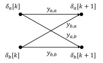
Figure 1: An example of GCS variables modeled into network flow for $n_{\delta}=2$.

GCS constructs network flow models for MIQPs depicted in Fig. 1. The binary variables $y_{a,b}$ and associated costs are placed on the edge $a\rightarrow b$ of the network, where $a,b\in\{1,...,n_{\delta}\}$. Let $\boldsymbol{z}_{a,b}=y_{a,b}\boldsymbol{x}_{a}$. If $y_{a,b}=1$, this edge is picked incurring a cost $\boldsymbol{z}_{a,b}^{T}\boldsymbol{Q}\boldsymbol{z}_{a,b}$ to the total cost at time $k$. If $y_{a,b}=0$, this edge is not selected and incurs $0$ cost to the total cost, indicating that the cost of selecting this edge is large. The variables $\boldsymbol{z}_{a,b}$ and $y_{a,b}$ are GCS variables readily available from its solution. For each edge $a\rightarrow b$ at time $k$, we recover its cost:

$$C_{a,b}[k]=\min(\boldsymbol{z}_{a,b}^{T}\boldsymbol{Q}\boldsymbol{z}_{a,b}/y_{a,b},\ L)$$ (29)

such that the cost on edge $a\rightarrow b$ is inverse proportional to $y_{a,b}$. $L$ is a large constant chosen by the user making the cost finite when $y_{a,b}=0$. We construct the following initial optimality cuts for the cost at time $k$, denoted by $z[k]$:

$$z[k]\geq 0,\ \ z[k]\geq C_{a,b}[k](\delta_{a}[k]+\delta_{b}[k+1]-1)\ \ \forall a,b\in\{1,...,n_{\delta}\}$$ (30)

and the total cost $z_{0}$ is the summation of $z[k]$’s.

6 Fast Algorithm for the Benders Master Problem

Since the BMP is an integer programming, its solving speed can be slow. [48] reported over 90% solving time on the BMP. If we do not aim at the global optimal solution of  (2), the BMP needs not to be solved to global optimality [23]. Therefore, heuristic approaches such as [27, 46] can be used to solve the BMP, termed Benders-type heuristics [15]. In this section, we present a fast heuristic algorithm to solve the BMP leveraging on the sparsity of feasibility cuts, avoiding expensive branch-and-bound procedures. Several previous works [53, 1, 20] analyzed or utilized sparsity of cuts to improve the computational performance. In particular, [20] connected the sparsity of feasibility cuts to the sparsity of constraint matrices. The matrices $\boldsymbol{A}$, $\boldsymbol{C}$ in this paper are sparse, and the feasibility cuts are found to be sparse. The sparsity is strengthened by the shifted feasibility cuts. It is found that more than 50% of the terms in $\widetilde{\boldsymbol{\Lambda}}_{p}^{mT}$, $\widetilde{\boldsymbol{\mathcal{V}}}^{mT}_{p}$ are zeros for our experimented problems.

Due to sparsity, a subset of $\boldsymbol{\delta}$ multiplied by non-zero coefficients in the feasibility cuts can be solved ahead of others. Leveraging this, a greedy-backtracking approach is proposed. We write out the structure of cuts. At iteration $p$, $\widetilde{\boldsymbol{\nu}}_{p}^{m}[k]=\boldsymbol{0}$, $\widetilde{\boldsymbol{\lambda}}_{p}^{m}[k]=\boldsymbol{0}$ for $k$ from a certain time step till the end of time horizon due to shifting. If a cut with certain $(p,m)$ has $\widetilde{\boldsymbol{\nu}}_{p}^{m}[1]\neq\boldsymbol{0}$ or $\widetilde{\boldsymbol{\lambda}}_{p}^{m}[0]\neq\boldsymbol{0}$, but $\widetilde{\boldsymbol{\nu}}_{p}^{m}[k]=\boldsymbol{0}$, $\forall k=2,...,N$, $\widetilde{\boldsymbol{\lambda}}_{p}^{m}[k]=\boldsymbol{0}$, $\forall k=1,...,N-1$, we place this cut into the index set $\{p_{0}\}$ and denote $\widetilde{\boldsymbol{\nu}}_{p_{0}}\triangleq\widetilde{\boldsymbol{\nu}}^{m}_{p}$, $\widetilde{\boldsymbol{\lambda}}_{p_{0}}\triangleq\widetilde{\boldsymbol{\lambda}}^{m}_{p}$. Define index sets $\{p_{1}\},...,\{p_{N-1}\}$ such that for $\{p_{i}\}$, $\widetilde{\boldsymbol{\nu}}_{p}[i+1]\neq\boldsymbol{0}$ or $\widetilde{\boldsymbol{\lambda}}_{p}[i]\neq\boldsymbol{0}$, but $\widetilde{\boldsymbol{\nu}}_{p}[k]=\boldsymbol{0}$, $\forall k=i+2,...,N$, $\widetilde{\boldsymbol{\lambda}}_{p}[k]=\boldsymbol{0}$, $\forall k=i+1,...,N-1$. Define $\widetilde{\boldsymbol{\Lambda}}_{p_{i}}$ and $\widetilde{\boldsymbol{\mathcal{V}}}_{p_{i}}$ according to  (20). Note that $\widetilde{\boldsymbol{\mathcal{V}}}_{p_{i}}[k]=\boldsymbol{0}$, $\forall k=i+1,...,N-1$, $\widetilde{\boldsymbol{\Lambda}}_{p_{i}}[k]=\boldsymbol{0}$, $\forall k=i+2,...,N-1$. The feasibility cuts can be parsed as:

$$\widetilde{\boldsymbol{\mathcal{V}}}_{p_{0}}[0]^{T}\boldsymbol{\delta}[0]\geq-S_{p_{0}} \hskip 8.5359ptp_{0}\in\{p_{0}\}$$

$$\widetilde{\boldsymbol{\mathcal{V}}}_{p_{1}}[0]^{T}\boldsymbol{\delta}[0]+\widetilde{\boldsymbol{\mathcal{V}}}_{p_{1}}[1]^{T}\boldsymbol{\delta}[1]\geq-S_{p_{1}} \hskip 8.5359ptp_{1}\in\{p_{1}\}$$

$$\vdots$$

$$\widetilde{\boldsymbol{\mathcal{V}}}_{p_{N-1}}[0]^{T}\boldsymbol{\delta}[0]+...+\widetilde{\boldsymbol{\mathcal{V}}}_{p_{N-1}}[N-1]^{T}\boldsymbol{\delta}[N-1]\geq-S_{p_{N-1}} \hskip 8.5359ptp_{N-1}\in\{p_{N-1}\}$$ (31)

where:

$$S_{p_{i}}\triangleq\sum_{k=0}^{i+1}\widetilde{\boldsymbol{\Lambda}}_{p_{i}}[k]^{T}\boldsymbol{\Theta}[k]$$ (32)

On the other hand, the optimality cuts  (25) and  (26) can be written as:

$$z_{0} \geq S_{q}-\sum_{k=0}^{N-1}\boldsymbol{\mathcal{V}}^{*}_{q}[k]^{T}\boldsymbol{\delta}[k],\ \ S_{q}\triangleq C_{q}-\boldsymbol{\Lambda}_{q}^{*T}\boldsymbol{\Theta},\ \ q\in\{q\}$$ (33a)

$$z_{0} \geq S_{qr}-\sum_{k=0}^{N-1}\boldsymbol{\mathcal{V}}_{qr}[k]^{T}\boldsymbol{\delta}[k],\ \,S_{qr}\triangleq C_{qr}(\boldsymbol{\Theta}),\ \ qr\in\{qr\}$$ (33b)

We write the index set of optimality cuts as $\{q\}\cup\{qr\}$, such that  (33a) and  (33b) are treated together. Based on their structure, we propose an algorithm to solve $\boldsymbol{\delta}[k]$ step by step into the future. The algorithm starts by solving $\boldsymbol{\delta}[0]$ at step $k=0$ from the following problem denoted by $P_{0}$:

$$\underset{\boldsymbol{\delta}[0]\in\{0,1\}^{n_{\delta}}}{\text{minimize}}\ \ z_{0}$$ (34)

s.t. $$\widetilde{\boldsymbol{\mathcal{V}}}_{p_{0}}[0]^{T}\boldsymbol{\delta}[0]\geq-S_{p_{0}}\ \ p_{0}\in\{p_{0}\}$$

$$z_{0}\geq S_{q}-\boldsymbol{\mathcal{V}}^{*}_{q}[0]^{T}\boldsymbol{\delta}[0]\ \ q\in\{q\}\cup\{qr\}$$

$P_{0}$ can be solved using appropriate algorithms. In many practical cases, the modes within one time-step can be easily enumerated (e.g. quadruped robots have $2^{4}$ contact modes). Solving $P_{0}$ is in the worst case checking each mode, and the solving time scales proportionally to the number of modes at each time-step. If the original BMP is feasible, then $P_{0}$ is feasible, as the variables and constraints are a subset of the original BMP. The solution to $P_{0}$, $\boldsymbol{\delta}^{*}[0]$, is then substituted into  (33a),  (33b), and the rest of  (31), such that the constant part $S_{p_{1}},...,S_{p_{N-1}}$ and $S_{q}$ are updated. In the next step, we solve problem $P_{1}$, having identical structure as $P_{0}$ except that $\widetilde{\boldsymbol{\mathcal{V}}}_{p_{0}}[0]$, $\boldsymbol{\mathcal{V}}^{*}_{q}[0]$ are replaced by $\widetilde{\boldsymbol{\mathcal{V}}}_{p_{1}}[1]$, $\boldsymbol{\mathcal{V}}^{*}_{q}[1]$, and $S_{p_{1}}$, $S_{q}$ are updated. This procedure is continued to solve $\boldsymbol{\delta}^{*}[1],...,\boldsymbol{\delta}^{*}[N-1]$. When solving $\boldsymbol{\delta}[k]$, we also include constraints involving $\boldsymbol{\delta}[k+1],...,\boldsymbol{\delta}[k+H]$ such that the choice of $\boldsymbol{\delta}[k]$ considers the feasibility of future $\boldsymbol{\delta}$’s $H$ steps ahead. For each constraint in $\{p_{k+1}\},...,\{p_{k+H}\}$, the following constraint is added:

$$\widetilde{\boldsymbol{\mathcal{V}}}_{p_{k}}[k]^{T}\boldsymbol{\delta}[k]+\sum_{i=1}^{h}\underset{\boldsymbol{\delta}[k+i]}{\text{max}}\{ \widetilde{\boldsymbol{\mathcal{V}}}_{p_{k+i}}[k+i]^{T}\boldsymbol{\delta}[k+i]\}\geq-S_{p_{k+h}},\ \ p_{k+h}\in\{p_{k+h}\}$$ (35)

Constraint  (35) gives the “least requirement” to $\boldsymbol{\delta}[k]$ for one constraint in $\{p_{k+h}\}$, such that the choice of $\boldsymbol{\delta}^{*}[k]$ guarantees feasibility for that constraint. However, the intersection of constraints can still cause infeasibility. When this happens, we backtrack $\boldsymbol{\delta}^{*}[k]$, and pick another less optimal solution. Obviously, this algorithm eventually finds a feasible solution if the original BMP is feasible. If backtracking does not happen, the number of investigated $P_{k}$ grows linearly with respect to $N$. Note that this algorithm does not guarantee global optimality solutions, as early decisions are made disregarding the decisions down the time horizon. Roughly speaking, early decisions are more essential for planning problems, hence this approach often finds high-quality solutions in our experiments.

7 Experiment

We test GBD-MPC on two different problems: controlling a cart-pole system to balance with moving soft contact walls, controlling a free-flying robot to navigate inside a maze. $G_{a}=0.1$ is used among the proposed and benchmark methods for all problems. $K_{feas}$ and $K_{opt}$ are chosen properly and reported for each experiment. For fair comparison with Gurobi’s MIQP solver, we use Gurobi’s QP solver for Benders subproblems. Other faster QP solvers [7] can further increase the speed. The algorithm is coded in C++, and tested in pybullet simulators [16] on a 12th Gen Intel Core i7-12800H × 20 laptop with 16GB memory.

7.1 Cart-pole with moving soft contact walls

We studied the problem to control a cart-pole system to balance between two moving soft contact walls. This problem is a more challenging version than the cart-pole with static walls problem prevail in literature [36, 19, 2, 9, 47]. The state variable $\boldsymbol{x}[k]\in\mathbb{R}^{4}$ where $x_{1}$ is the position of the cart, $x_{2}$ is the angle of the pole, and $x_{3}$, $x_{4}$ are their derivatives. Define $\lambda_{1}\geq 0$, $\lambda_{2}\geq 0$ as contact forces from the right and the left walls, and $f$ the horizontal actuation force to push the cart. The control input $\boldsymbol{u}[k]=\begin{bmatrix}f&\lambda_{1}&\lambda_{2}\end{bmatrix}^{T}\in\mathbb{R}^{3}$. The pendulum model is linearized around $x_{2}=0$ and discretized with a step size $dt=0.02s$. Readers are referred to [36] for the model of this system. Two binary variables $\boldsymbol{\delta}[k]\in\{0,1\}^{2}$ are defined to describe three contact scenarios: left, right, and no contact. The moving elastic pads with elastic coefficients $k_{1}$ and $k_{2}$ are located to the right of the origin at a distance of $d_{1}$, and to the left at $d_{2}$. The length of the pole is $l$. When the pole penetrates a wall ($x_{1}-lcos(x_{2})\geq d_{1}$ or $x_{1}-lcos(x_{2})\leq-d_{2}$), additional contact forces are generated at the tip of the pole. Otherwise, there is no contact force. This can be modeled as mixed-integer linear constraints and enforced using the standard big-M approach. Constraints also limit the cart position, velocity, pole angle, and angular velocity. This problem has $n_{x}=4$, $n_{u}=3$, $n_{z}=2$, $n_{c}=20$. The objective function tries to regulate the system to $x_{1}=x_{2}=0$.

At the beginning of each test episode, the pendulum is perturbed to $x_{2}=10\degree$ such that it will bump into the wall to regain balance. For the rest of each episode, the persistent random disturbance torque on the pole is generated from a Gaussian distribution $\mathcal{N}(0,8)\ N\cdot m$ . The system is constantly disturbed and has to frequently touch the wall for re-balance. The wall motion is generated by a random walk on top of a base sinusoidal motion $\Delta d=0.03sin(2\pi t)$. The wall motions are provided to the controller only at run-time through parameter $\boldsymbol{\theta}=\begin{bmatrix}d_{1}&d_{2}\end{bmatrix}$. For our experiments, we choose mass of cart $1.0kg$, mass of pole $0.4kg$, $l=0.6m$, $k_{1}=k_{2}=50N/m$, control limit $f_{max}=20N$, and angle limits $\pm\pi/2$. The weights are $\boldsymbol{Q}_{k}=\text{diag}(1,50,1,50)$, $\boldsymbol{R}_{k}=0.1\boldsymbol{I}_{3}$. The terminal cost $\boldsymbol{Q}_{N}$ is obtained by solving a discrete algebraic Ricatti equation. No warm-start from initial optimality cuts  (26) is necessary for this experiment.

Results We experimented with two different planning horizons: $10$ and $15$, having 20 and 30 binary variables, respectively. The data is collected from solved problems where at least one contact is planned, removing the cases when contact is not involved. The parameters are $K_{feas}=50$, $K_{opt}=40$ for $N=10$, and $K_{feas}=150$, $K_{opt}=40$ for $N=15$. Fig. 2 shows the solving speed in Hz during the first contact in the beginning $200ms$ of an episode, where GBD begins from an empty set of cuts but plans the first contact. After the first few iterations as cold-start, the solving speed increases over Gurobi. Note that the solving speed remains on average $50Hz$ without warm-start shown by the orange curve in subfigure A. The cost of GBD is similar to Gurobi. We highlight the data efficiency of GBD from the subfigures C, D showing less than 50 cuts can already provide good warm-starts for the initial conditions encountered along the trajectory. After the cold-start, GBD only picks up new cuts once in a while, as shown by the number of GBD iterations. On the other hand, the neural-network classifier proposed by [8] consumes over 90000 solved problems offline. Subfigure E show the histogram result of Monte-Carlo experiment for this scenario with 20 trajectories under random wall motions and disturbance torques, benchmark against the warm-started B&B algorithm (shown in subfigure F). The histogram shows the number of GBD iterations and their frequencies. Due to the warm-start, 99.2% of problem instances are solved within 5 GBD iterations, except for a few problems during the cold-start phase. The B&B algorithm still goes through more than 10$\times$ subproblems on average to converge compared to the GBD algorithm, despite the warm-starts reduce the number of solved subproblems over 50%.

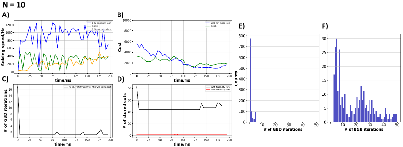
Figure 2: Cart-pole with soft walls simulated for $200ms$. A) solving speed comparison among proposed GBD, GBD without warm-start, and Gurobi, x-axis: simulation time in ms, y-axis: solving speed in Hz. B) Cost of proposed GBD and Gurobi. C) The number of GBD iterations. D) The number of cuts stored during the solving procedure. Blue curves: proposed GBD. Green curves: Gurobi. Orange curve: GBD without warm-start. Black curve: feasibility cuts, red curve: optimality cuts. E) Histogram result for this experiment with different $\boldsymbol{\Theta}$. x-axis: the number of GBD iterations. y axis: the count of problem instances. F) Same histogram result for Branch and Bound with warm-start [36].

Fig. 3 plots the solving speed and number of cuts for the same experiment but running continuously for a few seconds, when at least one contact is planned. Using a finite buffer avoids storing too many cuts and maintains the solving speed while still preventing cold-starts from frequently happening. This is justified by 77% of the cases and 74% cases resolved within one GBD iteration for $N=10$ and $15$. The solving speed of GBD is on average 2-3 times faster than Gurobi. For both $N=10$ and $15$, over 80% of the complete solving time is used on sub-QPs. Less than 20% of the solving time is on BMPs.

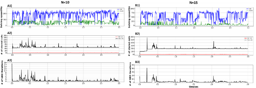
Figure 3: Solving speed, number of stored cuts, and number of GBD iterations for cart-pole with contact experiment. Left: N=10. Right: N=15. A1, B1 show the solving speed of GBD (blue curve) compared against Gurobi (green curve) in Hz. A2, B2 show the number of stored feasibility cuts (black curve) and optimality cuts (red curve). A3, B3 show the number of GBD iterations.

7.2 Free-flying robot navigating inside a maze

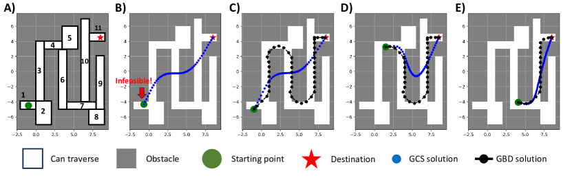
Figure 4: Maze and planned trajectories. Subfigure A): Starting point, destination, and convex patches. Subfigure B): Following GCS trajectory results in infeasibility. Subfigure C,D,E): Three snapshots of GBD planned trajectories with GCS solutions to construct initial optimality cuts.

To test the performance of GBD-MPC to plan trajectories with longer horizon using initial optimality cuts for warm-start, we studied the problem of free-flying robot navigating inside a 2D maze shown in the subfigure A of Fig. 4. The starting point is a green dot and the destination is in red star. During its traverse, the robot has to choose the correct direction to turn at each intersection. Therefore, the robot needs to plan globally optimal trajectories with long horizon. We choose $N=50$. The robot is modeled into a point mass with simple Newton 2nd law dynamics. The robot state $\boldsymbol{x}[k]\in\mathbb{R}^{4}$ include the 2-D positions $x$, $y$ and velocities $\dot{x}$, $\dot{y}$. The controls $\boldsymbol{u}[k]\in\mathbb{R}^{2}$ are $x$ and $y$ direction pushing forces. The maze is composed of 11 rectangular regions $\mathcal{R}_{e,i},i=1,...,11$ shown by the white areas in subfigure A) of Fig. 4, within which the robot is free to move around. The robot cannot move into the grey area that does not belong to any of the white rectangular regions. We define $\boldsymbol{\delta}[k]\in\{0,1\}^{11}$, such that $\delta_{i}[k]=1\Rightarrow(x[k],y[k])\in\mathcal{R}_{e,i}$ enforced by standard big-M formulation. Therefore, this problem has 550 binary variables. Robot mass $m=1$. Velocities and controls are all limited within $[-1,1]$. The discretization step size of the trajectory is $dt=0.65s$. The simulation environment propagates at a much shorter step size than $dt$. We choose $\boldsymbol{Q}_{k}=\text{diag}(1,1,0.2,0.2)$, $\boldsymbol{R}_{k}=0.1\boldsymbol{I}_{2}$, $K_{feas}=4000$, $K_{opt}=500$. We use GCS to generate initial optimality cuts  (30) to warm-start the Benders master problem. Our GCS formulation follows $5.5(a)-5.5(f)$ from [37], with additional linear dynamics constraint on each pair of edge variables $\boldsymbol{z}_{e}$, $\boldsymbol{z}^{\prime}_{e}$, solved by Gurobi. We do not run GCS for each new $\boldsymbol{\Theta}$ and often re-use the same solutions for different initial conditions, since it only represent a rough heuristics. As [35] claimed, GCS solving speed can benefit significantly from better solvers using graphic cards, but out of the scope of this paper. We exclude the GCS solving time and only report the solving time of GBD loops.

Results Subfigures C,D,E of Fig. 4 give three snapshots of the solved trajectory when the free-flying robot is navigating inside the maze. The blue dots depict the heuristic solutions from GCS. The black line with dots depict the GBD solutions with initial optimality cuts  (30) from GCS. We note that since GCS relaxation is too loose for this problem, its solutions are infeasible. If the robot follows GCS trajectories, it tries to enter the infeasible area of the maze. This is shown in subfigure B of Fig. 4. Therefore, using Benders cuts to tighten the GCS relaxation is necessary. With a planning horizon of 50, the GBD solutions successfully reach the goal. After the first few iterations that gather most of the necessary cuts, Benders MPC loop runs at 20Hz and re-plans the trajectory as the robot move forward. The first Benders loop takes about 200 iterations to converge with  (30). Without  (30), it usually takes more than 10 times more iterations to converge, demonstrating a significant improvement of the speed of convergence. The caveat is that  (30) may lead to sub-optimal solutions, which can be remedied by discounting $v_{pri,qr}$ towards $0$.

8 Conclusion

We proposed a hybrid MPC algorithm based on GBD that stores cuts to provide warm-starts for the new problem instances. A fast algorithm to solve the BMP is proposed. Heuristics is used to construct optimality cuts to plan trajectories at longer time horizons. Our algorithm shows competitive solving speeds to Gurobi in controlling the cart-pole system with randomly moving soft walls. It plans trajectories of time horizon 50 allowing the robot to navigate inside a maze.

References

- [1] Alfandari, L., Ljubić, I., da Silva, M.D.M.: A tailored benders decomposition approach for last-mile delivery with autonomous robots. European Journal of Operational Research 299(2), 510–525 (2022)
- [2] Aydinoglu, A., Wei, A., Posa, M.: Consensus complementarity control for multi-contact mpc. arXiv preprint arXiv:2304.11259 (2023)
- [3] Bemporad, A., Morari, M.: Control of systems integrating logic, dynamics, and constraints. Automatica 35(3), 407–427 (1999)
- [4] Benders, J.: Partitioning procedures for solving mixed-variables programming problems ‘. Numerische mathematik 4(1), 238–252 (1962)
- [5] Bertsimas, D., Tsitsiklis, J.N.: Introduction to linear optimization, vol. 6. Athena scientific Belmont, MA (1997)
- [6] Birge, J.R., Louveaux, F.: Introduction to stochastic programming. Springer Science & Business Media (2011)
- [7] Caron, S., Arnström, D., Bonagiri, S., Dechaume, A., Flowers, N., Heins, A., Ishikawa, T., Kenefake, D., Mazzamuto, G., Meoli, D., O’Donoghue, B., Oppenheimer, A.A., Pandala, A., Quiroz Omaña, J.J., Rontsis, N., Shah, P., St-Jean, S., Vitucci, N., Wolfers, S., @bdelhaisse, @MeindertHH, @rimaddo, @urob, @shaoanlu: qpsolvers: Quadratic Programming Solvers in Python (Dec 2023), https://github.com/qpsolvers/qpsolvers
- [8] Cauligi, A., Culbertson, P., Schmerling, E., Schwager, M., Stellato, B., Pavone, M.: Coco: Online mixed-integer control via supervised learning. IEEE Robotics and Automation Letters 7(2), 1447–1454 (2021)
- [9] Cauligi, A., Culbertson, P., Stellato, B., Bertsimas, D., Schwager, M., Pavone, M.: Learning mixed-integer convex optimization strategies for robot planning and control. In: 2020 59th IEEE Conference on Decision and Control (CDC). pp. 1698–1705. IEEE (2020)
- [10] Cleac’h, S.L., Howell, T., Schwager, M., Manchester, Z.: Fast contact-implicit model-predictive control. arXiv preprint arXiv:2107.05616 (2021)
- [11] Codato, G., Fischetti, M.: Combinatorial benders’ cuts for mixed-integer linear programming. Operations Research 54(4), 756–766 (2006)
- [12] Contreras, I., Cordeau, J.F., Laporte, G.: Benders decomposition for large-scale uncapacitated hub location. Operations research 59(6), 1477–1490 (2011)
- [13] Cordeau, J.F., Pasin, F., Solomon, M.M.: An integrated model for logistics network design. Annals of operations research 144, 59–82 (2006)
- [14] Cordeau, J.F., Stojković, G., Soumis, F., Desrosiers, J.: Benders decomposition for simultaneous aircraft routing and crew scheduling. Transportation science 35(4), 375–388 (2001)
- [15] Cote, G., Laughton, M.A.: Large-scale mixed integer programming: Benders-type heuristics. European Journal of Operational Research 16(3), 327–333 (1984)
- [16] Coumans, E., Bai, Y.: Pybullet, a python module for physics simulation for games, robotics and machine learning (2016)
- [17] Crainic, T.G., Hewitt, M., Rei, W.: Partial decomposition strategies for two-stage stochastic integer programs, vol. 88. CIRRELT (2014)
- [18] Dantzig, G.B., Wolfe, P.: Decomposition principle for linear programs. Operations research 8(1), 101–111 (1960)
- [19] Deits, R., Koolen, T., Tedrake, R.: Lvis: Learning from value function intervals for contact-aware robot controllers. In: 2019 International Conference on Robotics and Automation (ICRA). pp. 7762–7768. IEEE (2019)
- [20] Dey, S.S., Molinaro, M., Wang, Q.: Analysis of sparse cutting planes for sparse milps with applications to stochastic milps. Mathematics of Operations Research 43(1), 304–332 (2018)
- [21] Easwaran, G., Üster, H.: Tabu search and benders decomposition approaches for a capacitated closed-loop supply chain network design problem. Transportation science 43(3), 301–320 (2009)
- [22] Geoffrion, A.M.: Generalized benders decomposition. Journal of optimization theory and applications 10, 237–260 (1972)
- [23] Geoffrion, A.M., Graves, G.W.: Multicommodity distribution system design by benders decomposition. Management science 20(5), 822–844 (1974)
- [24] Glover, F.: Improved linear integer programming formulations of nonlinear integer problems. Management science 22(4), 455–460 (1975)
- [25] Heemels, W.P., De Schutter, B., Bemporad, A.: Equivalence of hybrid dynamical models. Automatica 37(7), 1085–1091 (2001)
- [26] Heemels, W., Schumacher, J.M., Weiland, S.: Linear complementarity systems. SIAM journal on applied mathematics 60(4), 1234–1269 (2000)
- [27] Hoang, L.: A fast and accurate algorithm for stochastic integer programming, applied to stochastic shift scheduling r. pacqueau, f. soumis. Les Cahiers du GERAD ISSN 711, 2440 (2012)
- [28] Hogan, F.R., Rodriguez, A.: Reactive planar non-prehensile manipulation with hybrid model predictive control. The International Journal of Robotics Research 39(7), 755–773 (2020)
- [29] Hooker, J.N., Ottosson, G.: Logic-based benders decomposition. Mathematical Programming 96(1), 33–60 (2003)
- [30] Hooker, J.N., Yan, H.: Logic circuit verification by benders decomposition. Principles and practice of constraint programming: the newport papers pp. 267–288 (1995)
- [31] Kuindersma, S., Deits, R., Fallon, M., Valenzuela, A., Dai, H., Permenter, F., Koolen, T., Marion, P., Tedrake, R.: Optimization-based locomotion planning, estimation, and control design for the atlas humanoid robot. Autonomous robots 40, 429–455 (2016)
- [32] Lazimy, R.: Mixed-integer quadratic programming. Mathematical Programming 22, 332–349 (1982)
- [33] Lin, X., Zhang, J., Shen, J., Fernandez, G., Hong, D.W.: Optimization based motion planning for multi-limbed vertical climbing robots. In: 2019 IEEE/RSJ International Conference on Intelligent Robots and Systems (IROS). pp. 1918–1925. IEEE (2019)
- [34] Magnanti, T.L., Wong, R.T.: Accelerating benders decomposition: Algorithmic enhancement and model selection criteria. Operations research 29(3), 464–484 (1981)
- [35] Marcucci, T., Petersen, M., von Wrangel, D., Tedrake, R.: Motion planning around obstacles with convex optimization. arXiv preprint arXiv:2205.04422 (2022)
- [36] Marcucci, T., Tedrake, R.: Warm start of mixed-integer programs for model predictive control of hybrid systems. IEEE Transactions on Automatic Control 66(6), 2433–2448 (2020)
- [37] Marcucci, T., Umenberger, J., Parrilo, P.A., Tedrake, R.: Shortest paths in graphs of convex sets. arXiv preprint arXiv:2101.11565 (2021)
- [38] McBride, R., Yormark, J.: An implicit enumeration algorithm for quadratic integer programming. Management Science 26(3), 282–296 (1980)
- [39] McDaniel, D., Devine, M.: A modified benders’ partitioning algorithm for mixed integer programming. Management Science 24(3), 312–319 (1977)
- [40] Menta, S., Warrington, J., Lygeros, J., Morari, M.: Learning q-function approximations for hybrid control problems. IEEE Control Systems Letters 6, 1364–1369 (2021)
- [41] Moroşan, P.D., Bourdais, R., Dumur, D., Buisson, J.: A distributed mpc strategy based on benders’ decomposition applied to multi-source multi-zone temperature regulation. Journal of Process Control 21(5), 729–737 (2011)
- [42] Noonan, F.: Optimal investment planning for electric power generation. (1975)
- [43] Optimization, G.: Mipgap (2023), https://www.gurobi.com/documentation/9.5/refman/mipgap2.html
- [44] Pereira, M.V., Pinto, L.M.: Stochastic optimization of a multireservoir hydroelectric system: A decomposition approach. Water resources research 21(6), 779–792 (1985)
- [45] Pereira, M.V., Pinto, L.M.: Multi-stage stochastic optimization applied to energy planning. Mathematical programming 52, 359–375 (1991)
- [46] Poojari, C.A., Beasley, J.E.: Improving benders decomposition using a genetic algorithm. European Journal of Operational Research 199(1), 89–97 (2009)
- [47] Quirynen, R., Di Cairano, S.: Tailored presolve techniques in branch-and-bound method for fast mixed-integer optimal control applications. Optimal Control Applications and Methods 44(6), 3139–3167 (2023)
- [48] Rahmaniani, R., Crainic, T.G., Gendreau, M., Rei, W.: The benders decomposition algorithm: A literature review. European Journal of Operational Research 259(3), 801–817 (2017)
- [49] Rei, W., Cordeau, J.F., Gendreau, M., Soriano, P.: Accelerating benders decomposition by local branching. INFORMS Journal on Computing 21(2), 333–345 (2009)
- [50] Rodriguez, J.A., Anjos, M.F., Côté, P., Desaulniers, G.: Milp formulations for generator maintenance scheduling in hydropower systems. IEEE Transactions on Power Systems 33(6), 6171–6180 (2018)
- [51] Saharidis, G.K., Boile, M., Theofanis, S.: Initialization of the benders master problem using valid inequalities applied to fixed-charge network problems. Expert Systems with Applications 38(6), 6627–6636 (2011)
- [52] Sontag, E.: Nonlinear regulation: The piecewise linear approach. IEEE Transactions on automatic control 26(2), 346–358 (1981)
- [53] Walter, M.: Sparsity of lift-and-project cutting planes. In: Operations Research Proceedings 2012: Selected Papers of the International Annual Conference of the German Operations Research Society (GOR), Leibniz University of Hannover, Germany, September 5-7, 2012. pp. 9–14. Springer (2013)
- [54] Warrington, J., Beuchat, P.N., Lygeros, J.: Generalized dual dynamic programming for infinite horizon problems in continuous state and action spaces. IEEE Transactions on Automatic Control 64(12), 5012–5023 (2019)
- [55] Watters, L.J.: Reduction of integer polynomial programming problems to zero-one linear programming problems. Operations Research 15(6), 1171–1174 (1967)
- [56] Zhang, J., Lin, X., Hong, D.W.: Transition motion planning for multi-limbed vertical climbing robots using complementarity constraints. In: 2021 IEEE International Conference on Robotics and Automation (ICRA). pp. 2033–2039. IEEE (2021)