Anomalous transport in long-ranged open quantum systems

Abstract

We consider a one-dimensional fermionic lattice system with long-ranged power-law decaying hopping with exponent $\alpha$. The system is further subjected to dephasing noise in the bulk. We investigate two variants of the problem: (i) an open quantum system where the setup is further subjected to boundary reservoirs enabling the scenario of a non-equilibrium steady state charge transport, and (ii) time dynamics of an initially localized single particle excitation in the absence of boundary reservoirs. In both variants, anomalous super-diffusive behavior is observed for $1<\alpha<1.5$, and for $\alpha>1.5$ the setup is effectively short-ranged and exhibits conventional diffusive transport. Our findings are supported by analytical calculations based on the multiple scale analysis technique that leads to the emergence of a fractional diffusion equation for the density profile. Our study unravels an interesting interplay between long-range interaction and dephasing mechanism that could result in the emergence of unconventional behaviour in open quantum systems.

Introduction. Quantum transport in low dimensional systems has been an active area of research specially due to the evidence of unconventional or anomalous behaviour Dhar (2008); Bertini et al. (2021); Landi et al. (2022); Purkayastha et al. (2018, 2021); Saha et al. (2023); Ljubotina et al. (2019); van Beijeren (2012); Ilievski et al. (2018); Lev et al. (2017); Ljubotina et al. (2023); Prosen and Žnidarič (2012); Agarwal et al. (2015); Rojo-Francàs et al. (2024); Chen et al. (2023). Research in this direction is not only of fundamental importance but can potentially have technological applications Jördens et al. (2008); Greiner et al. (2002); Jepsen et al. (2020); Atala et al. (2014); Syassen et al. (2008); Sieberer et al. (2016); Terraneo et al. (2002); Li et al. (2004). Remarkable experimental progress Joshi et al. (2022a); Bonato et al. (2016); Poyatos et al. (1996); Schäfer et al. (2020); Bloch et al. (2012); Maier et al. (2019); Barredo et al. (2016); Blatt and Roos (2012); Britton et al. (2012) in quantum devices and architecture has made it possible to realize one-dimensional systems which can in principle exhibit conductance ${\cal G}$ that scales differently from the conventional system size scaling ${\cal G}\propto 1/N$ with $N$ being the system size. Such a departure from diffusive behaviour is termed anomalous and conductance in such cases scales as ${\cal G}\propto 1/N^{\delta}$ where $0<\delta<1$ corresponds to super-diffusive transport and $\delta>1$ corresponds to sub-diffusive transport. Another widely employed alternate approach to classify transport is by studying the spread of wave-packets in the system Purkayastha et al. (2018); Schuckert et al. (2020); Gopalakrishnan et al. (2017a); Prelovšek et al. (2018); Lezama and Lev (2022); Bhakuni et al. (2024). The exponent associated with the scaling collapse of the wave function spread dictates the nature of anomalous transport or lack thereof. Often, there can be interesting relations between this exponent and the one associated with conductance scaling with system size Dhar et al. (2013); Li and Wang (2003); Liu et al. (2014).

Such anomalous transport is often predicted in setups with correlated or uncorrelated disorder Menu and Roscilde (2020); Okugawa et al. (2022); Chen et al. (2019); Girschik et al. (2013); Štrkalj et al. (2021); Poon et al. (2023). It has also been reported in interacting many-body quantum systems Fava et al. (2020); Kozarzewski et al. (2019); Brighi and Ljubotina (2024); Singh et al. (2021); Ljubotina et al. (2023); Bar Lev et al. (2015) or quantum systems subject to environmental effects Gopalakrishnan et al. (2017a); Prelovšek et al. (2018); Lezama and Lev (2022); Bhakuni et al. (2024). Despite a plethora of progress, a rigorous microscopic understanding of anomalous transport is still lacking. This is primarily due to the lack of simple platforms where both analytical calculations and state-of-the-art numerical simulations can be performed. Moreover, it is worth emphasising that most works studying anomalous transport consider short-range interacting systems. Some progress has recently been made in long-range systems where unconventional behaviour is reported Sarkar et al. (2024); Iubini et al. (2022a). Therefore, it is of paramount importance to explore the hidden mechanisms in setups with long-range coherent coupling, which results in anomalous behaviour. One such avenue is when long-range systems are subjected to dephasing mechanism and this is the central platform used in our work.

In this work, we study quantum transport properties in a one-dimensional long-range fermionic lattice system with the long-range hopping exponent denoted by $\alpha$. This setup is further sujected to dephasing noise, often called as Büttiker voltage probes (BVP), that acts at each lattice site. We first study the non-equilibrium steady state (NESS) scenario by connecting the setup by two boundary fermionic reservoirs one at each end. These boundary reservoirs result in the establishment of a NESS current. The given platform is amenable to exact results (non-perturbative and non-Markovian) in NESS. We investigate the system size scaling of conductance and observe super-diffusive transport regime when $1<\alpha<1.5$ and conventional diffusive regime when $\alpha>1.5$. We provide a compelling evidence for a relationship between system size scaling exponent of conductance ($\delta$) and long-range hopping exponent ($\alpha$). We then characterize the transport by performing quantum dynamics study of single-particle excitation in the absence of the fermionic boundary reservoirs but retaining the dephasing mechanism. The exponent ($\eta$) associated with the space-time collapse of the single particle density profile is found to be super-diffusive for $1<\alpha<1.5$ and diffusive for $\alpha>1.5$. We support these findings by obtaining a fractional diffusion equation for the density profile following a multiple scale analysis technique Bender and Orszag (1999). We further obtain a relationship between $\eta$ and $\alpha$. This along with the relationship between $\eta$ and $\delta$, known in the context of Lévy flights Dhar et al. (2013); Iubini et al. (2022b), establishes a relation between $\delta$ and $\alpha$ which is fully in agreement with our NESS analysis.

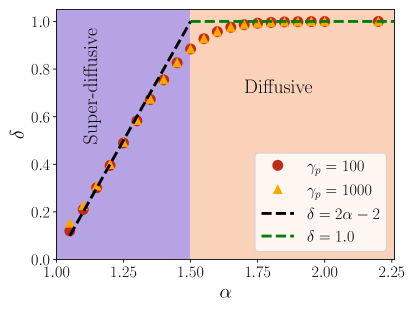
Figure 1: Plot for the system size scaling exponent $\delta$ for NESS conductance with long-range hopping exponent $\alpha$. The exponent $\delta$ is extracted by computing conductance for three large system sizes, $N=8192$, $11585$, and $N=16384$. The transition from super-diffusive to diffusive transport regime is observed when $\alpha\sim 1.5$. We plot results for two different choices for $\gamma_{p}$, $\gamma_{p}=100,1000$. We set $\gamma=J=1$. For the plot we choose, $\mu=\epsilon^{\alpha}_{lb}+0.5$, where $\epsilon^{\alpha}_{lb}$ denotes the energy corresponding to the lower band edge for the given $\alpha$. However note that, in the strong $\gamma_{p}$ limit, the scaling exponent $\delta$ is almost independent of the value of the equilibrium chemical potential $\mu$.

Long-range lattice setup and NESS transport. We consider a one-dimensional fermionic lattice chain with long-range hopping. The Hamiltonian is given by, Purkayastha et al. (2021); Sarkar et al. (2024)

$$\hat{{\cal H}}_{S}=-\sum\limits_{m=1}^{N}\frac{J}{m^{\alpha}}\Bigg{[}\sum\limits_{r=1}^{N-m}\hat{c}^{\dagger}_{r}\hat{c}_{r+m}+\hat{c}^{\dagger}_{r+m}\hat{c}_{r}\Bigg{]},$$ (1)

where $N$ is the system size, $\hat{c}_{r}^{\dagger}(\hat{c}_{r})$ is the fermionic creation (annihilation) operator for the $r$-th site, and $\alpha$ is the long-range hopping exponent. To understand the steady-state transport properties, the lattice chain is further connected to a source and a drain reservoir at its two ends, and these reservoirs are maintained at chemical potentials $\mu_{S}$ and $\mu_{D}$, respectively. The interaction between the system and each reservoir, whose strength is denoted by $\gamma$, is chosen to be bilinear and number-conserving. Here, for simplicity, we consider the wide-band limit of the reservoirs which implies frequency independent density of states. In addition to the boundary reservoirs, at each lattice site, we attach Büttiker voltage probes (BVP) with uniform coupling strength denoted by $\gamma_{p}$. This is done to mimic processes where the phase coherence of particles built during Hamiltonian evolution is lost due to inevitable surroundings D’Amato and Pastawski (1990); Kilgour and Segal (2016); Chiaracane et al. (2022). Such an approach is widely employed to understand effective many-body transport Roy and Dhar (2007); Saha et al. (2022). It is to be borne in mind that BVP’s are essentially themselves similar to the boundary reservoirs discussed above with the difference being their chemical potentials (denoted by $\mu_{i},i=1,2,\cdots N$ with $i$ stands for the index for the lattice site) are carefully engineered to ensure zero particle NESS current. The temperature however for the boundary reservoirs and the BVP’s are always considered to be the same. Note that we do not assume any restriction on the magnitude of the coupling between the system and the boundary reservoirs/probes. We are interested in studying the NESS electronic conductance to characterize transport. We focus here in the linear response regime and set for boundary reservoirs $\mu_{D}=\mu$, $\mu_{S}=\mu+\delta\mu$, and for the BVP’s $\mu_{i}=\mu+\delta\mu_{i},i=1,2,\cdots N$. At zero temperature, the conductance corresponding to the left to right charge current can be exactly obtained as Saha et al. (2022)

$${\cal G}(\mu) = \gamma^{2}|G_{1N}(\mu)|^{2}$$ (2)

$$+ \gamma^{2}\gamma_{p}\sum_{n,j=1}^{N}|G_{Nn}(\mu)|^{2}\,{\cal W}_{nj}^{-1}(\mu)\,|G_{j1}(\mu)|^{2},$$

where $G_{ij}(\omega)$ is the matrix element of the $N\times N$ dressed retarded Green’s function matrix ${G}(\omega)$ for the lattice, which can be written as,

$${G}(\omega)=\Big{[}\omega\,{I}-{h}_{S}-{{\bf\Sigma}}_{L}(\omega)-{{\bf\Sigma}}_{R}(\omega)-{{\bf\Sigma}}_{P}(\omega)\Big{]}^{-1}$$ (3)

with ${I}$ being the $N\times N$ identity matrix, ${h}_{S}$ being the single particle $N\times N$ matrix corresponding to the lattice Hamiltonian and defined as $\hat{\cal H}_{S}=\sum_{l,m=1}^{N}[{h}_{S}]_{lm}\hat{c}_{l}^{\dagger}c_{m}$ in Eq. (1), ${\bf\Sigma}_{\alpha}(\omega),\alpha=L,R,P$ are the self-energy matrices for the left reservoir, right reservoir and the BVPs. The self-energy matrices are diagonal with ${\bf\Sigma}_{L}(\omega)|_{11}=-i\gamma/2$, ${\bf\Sigma}_{R}(\omega)|_{NN}=-i\gamma/2$, and ${\bf\Sigma}_{P}(\omega)|_{jj}=-i\gamma_{p}/2,\,j=1,2,\cdots N$. The matrix elements of $N\times N$ matrix ${\cal W}(\omega)$ in Eq. (2) are given by Saha et al. (2022) (we suppress the argument in ${\cal W}$ and $G$ for the sake of brevity)

$${\cal W}_{ij} = -\gamma_{p}|G_{ij}|^{2}\quad\forall\quad n\neq j$$

$${\cal W}_{ii} = \gamma\Big{(}|G_{i1}|^{2}+|G_{iN}|^{2}\Big{)}+\gamma_{p}\sum_{j\neq n}^{N}|G_{nj}|^{2}\,\,\forall\,\,n\neq j.$$

(4)

The zero particle NESS current from each of the BVP ensures a unique chemical potential value at each lattice site and is given by Saha et al. (2022)

$$\mu_{i}=\mu_{S}+\gamma\,\gamma_{p}\,(\mu_{D}-\mu_{S})\,\sum_{j=1}^{N}{\cal W}_{ij}^{-1}\,|G_{jN}|^{2},$$ (5)

where $i=1,2,\cdots N$ and ${\cal W}$ is given in Eq. (4). Having the expressions for conductance [Eq. (2)] and chemical potential [Eq. (5)] in hand, we now provide the results based on extensive numerical simulations.

In the context of long-range systems, a natural question one may ask is the behavior of system size scaling exponent $\delta$ with respect to long-range hopping exponent $\alpha$. This is demonstrated in Fig. 1. In the limit of large probe coupling strength ($\gamma_{p}\gg J,\gamma$) we observe a super-diffusive transport regime $(0<\delta<1)$ for $1<\alpha<1.5$. Our findings indicate that the relationship between $\delta$ and $\alpha$ in the super-diffusive regime is $\delta\approx 2\alpha-2$. We further find a diffusive transport regime i.e., $\delta=1$ for $\alpha>1.5$. This remarkable crossover in the nature of transport is rooted in the effectively short-ranged interaction when $\alpha>1.5$. In contrast, an interesting interplay between the dephasing noise introduced by the BVPs and the effectively long-ranged hopping ($\alpha<1.5$) gives rise to a faster than diffusive or super-diffusive transport regime. Remarkably similar observations for transport were recently reported for Lindbladian systems Sarkar et al. (2024).

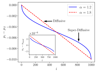
Figure 2: Plot for the local chemical potential $\mu_{i}$ (subtracted by the chemical potential of the source end $\mu_{S}$) profile as given in Eq. (5) for $\alpha=1.2$ (blue-solid), and $\alpha=1.8$ (red-dashed). The distinct line shapes of the profiles in the two transport regimes can be clearly seen here. We choose the value of $\mu_{S}$ to be the energy corresponding to the middle of the band, i.e., for $\alpha=1.2$, we choose $\mu_{S}=-4.87$ and for $\alpha=1.8$, we choose $\mu_{S}=-1.08$, and $\delta\mu=0.01$. The system size $N=1000$. We choose $\gamma_{p}=1000$. The inset represents the local occupation number $n_{i}$ (subtracted by the density at the middle of the lattice $n_{mid}$ to clearly demonstrate the density profile) vs $i$ in the two regimes. $n_{mid}$ depends on the chemical potential and the density of states, which is different in the two regimes.

In Fig. 2, we demonstrate the local chemical potential profile for two different values of $\alpha$, one within the super-diffusive regime and one within the diffusive regime. For $\alpha>1.5$, we notice a linear shape, which is a hallmark of conventional diffusive transport Dhar et al. (2013), whereas for $\alpha<1.5$, the shape is nonlinear, which is a fingerprint of anomalous transport Dhar et al. (2013). The inset of Fig. 2 demonstrates the local occupation number in the two distinct regimes. Given the detailed understanding of transport regimes when boundary reservoirs are attached, it is natural to explore the possible relation with the density profile evolution in the absence of reservoirs (but retaining the dephasing mechanism).

Time dynamics of single particle density profile: We now study the quantum dynamics of single particle excitation for the long-range lattice setup in the absence of the boundary reservoirs while keeping the dephasing mechanism intact. We model the lattice and this dephasing mechanism by a Lindblad quantum master equation (LQME) Turkeshi and Schiró (2021); Gopalakrishnan et al. (2017b); Žnidarič (2010); Sarkar et al. (2024); Dolgirev et al. (2020a); Tupkary et al. (2022); Nathan and Rudner (2020); Maniscalco et al. (2004); Manzano (2020); Palmero et al. (2019); Lindblad (1976), given as (setting $\hbar=1$)

$$\frac{d\hat{\rho}}{dt}=-i[\hat{{\cal H}}_{S},\hat{\rho}]+\kappa\sum_{i=1}^{N}\Bigg{[}\hat{n}_{i}\,\hat{\rho}\,\hat{n}_{i}-\frac{1}{2}\Big{\{}\hat{n}_{i}^{2},\hat{\rho}\Big{\}}\Bigg{]}$$ (6)

where the first term in Eq. (6) is responsible for unitary evolution with $\hat{\cal H}_{S}$ given by Eq. (1), and the second term mimics the dephasing mechanism with $\hat{n}_{i}=\hat{c}_{i}^{\dagger}\hat{c}_{i}$ being the number operator corresponding to the $i$-th site. $\kappa$ represents the effective coupling strength characterising dephasing Turkeshi and Schiró (2021); Gopalakrishnan et al. (2017b); Žnidarič (2010); Sarkar et al. (2024); Dolgirev et al. (2020a); Bhakuni et al. (2024). Note that, although the lattice Hamiltonian $\hat{\cal H}_{S}$ in Eq. (6) is quadratic, the open quantum system version as written in Eq. (6) is far from being trivial. This is due to the presence of dephasing terms, which results in the appearance of a quartic term in the LQME Dolgirev et al. (2020a). For such a setup, we are interested in studying the time dynamics of a single-particle density profile $P(x,t)$ which is initially localized at the middle site of the lattice. Note that, here we introduced a new variable $x=i-(N+1)/2$ so as to have the excitation at $x=0$ and we assume the lattice size $N$ to be odd here, without any loss of generality. Obtaining $P(x,t)$ directly following the LQME in Eq. (6) is computationally expensive since one has to deal with large $N^{2}\times N^{2}$ matrices. This issue can be circumvented by following a unitary unraveling procedure Wiseman and Diósi (2001); Salgado and Sánchez-Gómez (2002) of Eq. (6) which makes it more computationally feasible. The unraveling is carried out by introducing classical delta-correlated Gaussian noise at each lattice site Dolgirev et al. (2020b); Bhakuni et al. (2024). The total Hamiltonian can therefore be written as

$$\hat{{\cal H}}(t)={\cal H}_{S}+\sum_{l=1}^{N}\xi_{l}(t)\,n_{l},$$ (7)

with $\langle\xi_{l}(t)\rangle=0$, and $\langle\xi_{l}(t)\,\xi_{p}(t^{\prime})\rangle=\kappa\,\delta_{lp}\,\delta(t-t^{\prime})$, where recall that $\kappa$ is the dephasing strength. For each noise realization, we perform the dynamics governed by $\hat{\cal H}(t)$ in Eq. (7), and the quantity of interest is obtained by averaging over different noise realizations. For a single noise realization, the single particle density profile is obtained as $P_{\xi}(x,t)=|\psi^{\xi}_{x}(t)|^{2}$, with

$$\psi^{\xi}_{x}(t)={G}_{\xi}\Big{(}\frac{N+1}{2}+x,t\Big{|}\frac{N+1}{2},0\Big{)},$$ (8)

where

$$G_{\xi}\Big{(}x_{1},t_{1}\big{|}x_{0},t_{0}\Big{)}=\Big{\langle}x_{1}\big{|}{\cal T}e^{-i\int_{t_{0}}^{t_{1}}h(t^{\prime})dt^{\prime}}\big{|}x_{0}\big{\rangle}$$ (9)

is the single-particle unitary propagator with $h(t)$ being the single particle Hamiltonian, defined as $\hat{\cal H}(t)=\sum_{l,m=1}^{N}h_{lm}(t)\hat{c}_{l}^{\dagger}\hat{c}_{m}$, following Eq. (7). Here ${\cal T}$ is the time-ordered operator. Note that, the variable $x$ goes from $(-N+1)/2$ to $(N\!-\!1)/2$. We evaluate the full propagator by performing infinitesimal time propagation in steps of $dt$ and write ${\cal T}e^{-i\int_{t_{i}}^{t_{i}+dt}h(t^{\prime})dt^{\prime}}\approx e^{-i\big{(}h_{S}dt+\sqrt{dt}\,\mathcal{M}(t_{i})\big{)}}$ where $\mathcal{M}(t_{i})$ is a $N\times N$ diagonal noise matrix at time $t_{i}$ with $m$-th entry of the matrix corresponds to the value of the uncorrelated noise at the $m$th site i.e. $\langle\mathcal{M}_{m,m}(t_{i})\rangle=0$ and $\langle\mathcal{M}_{m,m}(t_{i})\mathcal{M}_{n,n}(t_{j})\rangle=\kappa\,\delta_{mn}\,\delta_{ij}$. Finally, the single-particle density profile at a particular time instant can be obtained by averaging over different noise trajectories, i.e., $P(x,t)=\overline{P_{\xi}(x,t)}$. We first present the numerical results for $P(x,t)$. In Fig. 3(a) and (b), we show that the numerics obeys the space-time scaling collapse of $P(x,t)$ of the form

$$P(x,t)=\frac{1}{(D_{\alpha}t)^{\eta}}\,f\bigg{(}\frac{x}{(D_{\alpha}t)^{\eta}}\bigg{)}.$$ (10)

In the regime $1<\alpha<1.5$, we find $\eta\approx 1/(2\alpha-1)$ and for $\alpha>1.5$, we get $\eta\approx 1/2$. In what follows we show that one can analytically obtain a fractional diffusion equation for the single particle density profile that provides both the scaling exponents and also the scaling function $f(x/(D_{\alpha}t)^{\eta})$ given in Eq. (10).

To arrive at the fractional-diffusion equation, we use the multiple-scale analysis technique. We focus on the correlator $D_{m,n}(t)\equiv\langle\hat{c}_{m}^{\dagger}(t)\hat{c}_{n}(t)\rangle$, where both $m$ and $n$ goes from $(-N+1)/2$ to $(N\!-\!1)/2$. Note that the diagonal element $D_{m,m}(t)$ for a single particle problem gives the density profile $P(m,t)$ at time $t$. We write down the equation of motion for $D_{m,n}(t)$ following the LQME in Eq. (6) and obtain

$$\frac{d}{dt}D_{m,n}(t) = iJ\sum_{l\neq 0}\left(\frac{D_{m,n+l}(t)-D_{m+l,n}(t)}{|l|^{\alpha}}\right)$$ (11)

$$+ \kappa\,(\delta_{m,n}-1)D_{m,n}(t).$$

In the strong dephasing limit $(\kappa\gg J)$, and using a perturbative expansion of $D_{m,n}$ in terms of a small parameter $\epsilon$, we obtain the following fractional-diffusion equation for the density profile (see Appendix A for the details of the derivation)

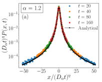
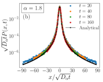
Figure 3: (Color online) Time-dynamics shown as a scaling collapse for the single-particle density profile that is initially localized at the middle site of the lattice for (a) $\alpha=1.2$ and (b) $\alpha=1.8$. For (a) the collapse happens for $\eta\approx 1/(2\alpha-1)$ and for $\alpha=1.2$, $\eta\approx 0.71$ . For both the figures, we choose $N=201,\gamma_{p}=50$, and noise average over 60 different realizations are performed with $dt=0.01$ (Note, we require $dt\ll{\rm min}\{J^{-1},\kappa^{-1}\}$). The black curves are analytically derived scaling functions as mentioned in Eq. (13) along with finite time corrections Schuckert et al. (2020) that are crucial to describe the heavy tails in the diffusive regime as shown in (b) which survive for algebraically long times. The corrections explicitly depend on time, and in particular, for (b), the black curve corresponds with $t=160$.

$$\frac{d}{dt}D_{m,m}(t)=\frac{2J^{2}}{\kappa}\sum_{l\neq 0}\left(\frac{D_{m+l,m+l}(t)-D_{m,m}(t)}{|l|^{2\alpha}}\right).$$ (12)

Note that, in the nearest neighbour case ($\alpha\to\infty$), the summation in Eq. (12) is restricted to $l=\pm 1$ which leads to a conventional diffusion equation with diffusion constant $\Delta=2J^{2}/\kappa$. Remarkably, Eq. (12) possesses interesting scaling forms Schuckert et al. (2020) in both the regimes $1<\alpha<1.5$ and $\alpha>1.5$. The scaling functions are given by:

$$f\bigg{(}z=\frac{x}{(D_{\alpha}t)^{\eta}}\bigg{)}\approx\begin{cases}F_{\alpha}(z),\hskip 34.14322pt1<\alpha<1.5\\ G(z),\hskip 39.83368pt\alpha>1.5\end{cases}$$ (13)

with $\eta=1/(2\alpha-1)$ for $1<\alpha<1.5$, and $\eta=1/2$ for $\alpha>1.5$. Here,

$$F_{\alpha}(z) = \int_{-\infty}^{\infty}\frac{dk}{2\pi}e^{-|k|^{2\alpha-1}}e^{izk},\quad\,G(z)=\frac{e^{-z^{2}/4}}{2\sqrt{\pi}}.\,\,\,\,$$ (14)

There are finite time corrections to these scaling functions Schuckert et al. (2020), which lead to heavy tails even when $\alpha>1.5$, i.e., corrections in $G(z)$ given in Eq. (14) (see Appendix B for details). $D_{\alpha}$ is a generalized diffusion constant, which is given by $D_{\alpha}\approx-2\Delta\Gamma(1-2\alpha)\sin(\pi\alpha)$ for $1<\alpha<1.5$ with $\Gamma$ being the Gamma function, while $D_{\alpha}\approx\Delta/(2\alpha-3)$ for $\alpha>1.5$. For $\alpha\gg 1.5$, the heavy tails would vanish and $D_{\alpha}\approx\Delta$. In Fig. 3, we demonstrate remarkable agreement between the scaling form (with no phenomenological parameters) given in Eq. (13) (with corrections) and our extensive numerical simulations based on stochastic unraveling Eq.(7) .

An important question that naturally emerges is the relation between the system-size scaling exponent of steady state conductance ($\delta$) and the exponent $\eta$ associated with the space-time collapse. We note that the anomalous super-diffusive transport in long-range systems is often governed by Lévy flights Schuckert et al. (2020); Dhar et al. (2013); Iubini et al. (2022b). In our case, we find an intriguing connection with a well known random walk model in low-dimensional systems, i.e., Lévy walk Zaburdaev et al. (2015). The typical space-time scaling in the central region of a pulse dictated by Lévy walker is $x\sim t^{1/\beta}$ where $\beta$ is the exponent associated with the time of flight distribution of a Lévy walker Dhar et al. (2013). If such a system is connected to boundary reservoirs, then the system size scaling of conductance Dhar et al. (2013) is given by $N^{1-\beta}$. For our setup, following the time dynamics of single particle density profile, we find that $\beta=2\alpha-1$ [Eq. (13)], which immediately gives a relation between the exponents $\delta$ and $\alpha$ as $\delta=2\alpha-2$. This perfectly matches with our numerical predictions on transport.

Summary. In summary, we have studied quantum transport properties in one-dimensional long-range fermionic system subjected to dephasing noise. The interesting interplay between the incoherent dephasing mechanism and the coherent long-range hopping, results in an anomalous behaviour. This clear departure from conventional diffusive transport is manifested both in NESS transport and in density profile dynamics. An interesting byproduct of our finding is that when $\alpha=5/4$, we get $\eta=2/3$ which is associated with the Kardar-Parisi-Zhang universality class Kardar et al. (1986); Takeuchi (2018); Spohn (2014); Prähofer and Spohn (2004) at least as far as exponents in space-time correlations are concerned. Furthermore, the density profile dynamics was shown to emerge from a fractional diffusion equation which was derived following the multiple scale analysis technique. This aided in further cementing the relationship between conductance scaling exponent $\delta$ and the long-range hopping exponent $\alpha$.

Recent theoretical Schuckert et al. (2020) and experimental Joshi et al. (2022b) advances in interacting quantum spin-chains have reported such anomalous transport by studying unequal space-time spin-spin correlators. Our work reveals a possible intriguing connection between such interacting quantum systems and systems subjected to dephasing noise mechanisms. Bringing out this interesting connection is an important future direction. The complex interplay between long-range hopping, dephasing noise in the bulk and boundary reservoirs can have interesting implications in several quantities such as entanglement entropy Kehrein (2024); Saha et al. (2024); Glatthard (2024), negativity Plenio (2005), and quantum fluctuations Song et al. (2011); Klich and Levitov (2009).

Appendix A Derivation of the fractional diffusion equation from the Lindblad QME in Eq. (6)

In this appendix, we provide a derivation for the fractional diffusion equation for the long-range setup following the Lindblad QME given in Eq. (6). The derivation is based on the multiple scale analysis technique Bender and Orszag (1999). An alternative route is that of renormalization group technique which was recently employed to derive a diffusion equation Fujimoto et al. (2022). We start with the time evolution of the density matrix which is given by,

$$\frac{d\hat{\rho}(t)}{dt}=-i[\hat{\cal H}_{S},\hat{\rho}(t)]+\kappa\sum_{i=(-N+1)/2}^{(N-1)/2}\left(\hat{n}_{i}\rho(t)\hat{n}_{i}-\frac{1}{2}\{\hat{n}_{i}^{2},\hat{\rho}(t)\}\right).$$ (15)

Here we have consider the middle site of the lattice as origin. $\hat{\cal H}_{S}$ is the long-range lattice Hamiltonian as given in Eq. (1), $\kappa$ is the effective dephasing strength. In what follows, we show that in the large dephasing $\kappa$ limit, the single-particle density profile obeys a fractional diffusion equation. For that purpose, we focus on the correlator $D_{m,n}(t)\equiv\langle\hat{c}_{m}^{\dagger}(t)\hat{c}_{n}(t)\rangle$ and write down its equation of motion following the LQME in Eq. (15). Note that, for the single particle problem the diagonal elements of $D_{m,m}(t)$ gives the density profile $P(m,t)$ at time $t$. We obtain,

$$\begin{split}\frac{d}{dt}D_{m,n}(t)=&iJ\sum_{l\neq 0}\left(\frac{D_{m,n+l}(t)-D_{m+l,n}(t)}{|l|^{\alpha}}\right)+\kappa\,(\delta_{m,n}-1)D_{m,n}(t).\end{split}$$ (16)

We change the variables to $\tau=\kappa\,t$, and work in the strong dephasing limit i.e., $\kappa\gg J$ where recall that $J$ is the hopping strength. We introduce a parameter $\epsilon_{l}=\frac{J\kappa^{-1}}{l^{\alpha}}$, with $l\geq 1$ and receive,

$$\frac{d}{d\tau}D_{m,n}(\tau)= i\sum_{l\neq 0}\epsilon_{|l|}\,\bigg{(}D_{m,n+l}(\tau)-D_{m+l,n}(\tau)\bigg{)}+\lambda_{m,n}D_{m,n}(\tau),$$ (17)

where $\lambda_{m,n}=\delta_{m,n}-1$. We will expand the solution $D_{m,n}$ in terms of a small parameter

$$\epsilon=\sum_{l\geq 1}\epsilon_{l}=\frac{J}{\kappa}\xi(\alpha),$$ (18)

where $\xi(\alpha)$ is the Riemann-Zeta function which converges for $\alpha>1$. We first seek for a convergent solution for $D_{m,n}(\tau)$ by expanding it in powers of $\epsilon$ as,

$$D_{m,n}(\tau)=D_{m,n}^{(0)}(\tau)+\epsilon\,D_{m,n}^{(1)}(\tau)+\epsilon^{2}\,D_{m,n}^{(2)}(\tau)+...$$ (19)

Substituting this in Eq. (17), and matching order by order of $\epsilon$, we obtain:

$$\frac{d}{d\tau}D_{m,n}^{(0)}(\tau)= \lambda_{m,n}D_{m,n}^{(0)}(\tau),$$ (20)

$$\begin{split}\epsilon\frac{d}{d\tau}D_{m,n}^{(1)}(\tau)=&\epsilon\,\lambda_{m,n}\,D_{m,n}^{(1)}(\tau)+i\sum_{l\neq 0}\epsilon_{|l|}\,\Big{(}D_{m,n+l}^{(0)}(\tau)-D_{m+l,n}^{(0)}(\tau)\Big{)},\end{split}$$ (21)

$$\begin{split}\epsilon^{2}\frac{d}{d\tau}D_{m,n}^{(2)}(\tau)=&\epsilon^{2}\lambda_{m,n}D_{m,n}^{(2)}(\tau)+i\sum_{l\neq 0}\epsilon_{|l|}\epsilon\left(D_{m,n+k}^{(1)}(\tau)-D_{m+k,n}^{(1)}(\tau)\right),\end{split}$$ (22)

$$\vdots$$ (23)

$$\begin{split}\epsilon^{a}\frac{d}{d\tau}D_{m,n}^{(a)}(\tau)=&\epsilon^{a}\lambda_{m,n}D_{m,n}^{(a)}(\tau)+i\sum_{l\neq 0}\epsilon_{|l|}\epsilon^{a-1}\left(D_{m,n+k}^{(a-1)}(\tau)-D_{m+k,n}^{(a-1)}(\tau)\right),\end{split}$$ (24)

where the symbol $a>1$ indicates $a$-th order in $\epsilon$. We re-write the above equations as,

$$\frac{d}{d\tau}D_{m,n}^{(0)}(\tau)= \lambda_{m,n}D_{m,n}^{(0)}(\tau),$$ (25)

$$\begin{split}\frac{d}{d\tau}D_{m,n}^{(1)}(\tau)=&\lambda_{m,n}D_{m,n}^{(1)}(\tau)+\frac{i}{\epsilon}\sum_{l\neq 0}\epsilon_{|l|}\,\left(D_{m,n+l}^{(0)}(\tau)-D_{m+l,n}^{(0)}(\tau)\right),\end{split}$$ (26)

$$\begin{split}\frac{d}{d\tau}D_{m,n}^{(2)}(\tau)=&\lambda_{m,n}D_{m,n}^{(2)}(\tau)+\frac{i}{\epsilon}\sum_{l\neq 0}\epsilon_{|l|}\,\left(D_{m,n+l}^{(1)}(\tau)-D_{m+l,n}^{(1)}(\tau)\right),\end{split}$$ (27)

$$\vdots$$ (28)

$$\begin{split}\frac{d}{d\tau}D_{m,n}^{(a)}(\tau)=&\lambda_{m,n}D_{m,n}^{(a)}(\tau)+\frac{i}{\epsilon}\sum_{l\neq 0}\epsilon_{|l|}\left(D_{m,n+l}^{(a-1)}(\tau)-D_{m+l,n}^{(a-1)}(\tau)\right).\end{split}$$ (29)

Let us now consider the initial condition to be such that $D_{m,n}(\tau=0)=D_{m,n}^{(0)}(\tau=0)$. This makes $D_{m,n}^{(a)}(\tau=0)=0$ for all $a>0$. Solving the $0^{th}$ order equation, we have

$$D_{m,n}^{(0)}(\tau)= A_{m,n}e^{\lambda_{m,n}\tau},$$ (30)

$$D_{m,n}^{(1)}(\tau)= \frac{ie^{\lambda_{m,n}\tau}}{\epsilon}\int_{0}^{\tau}dt^{\prime}\,e^{-\lambda_{m,n}t^{\prime}}\sum_{l\neq 0}\epsilon_{|l|}\left(D_{m,n+l}^{(0)}(t^{\prime})-D_{m+l,n}^{(0)}(t^{\prime})\right).$$ (31)

Now, substituting the $0^{th}$ order solution into $1^{st}$ order equation, we get for the diagonal and non-diagonal elements of $D^{(1)}_{m,n}(\tau)$ as

$$D_{m,m}^{(1)}(\tau)= \frac{i(1-e^{-\tau})}{\epsilon}\sum_{l\neq 0}\epsilon_{|l|}\left(A_{m,m+l}-A_{m+l,m}\right)$$ (32)

$$\begin{split}D_{m,m+b}^{(1)}(\tau)=&\frac{i\tau e^{-\tau}}{\epsilon}\sum_{l\neq 0,-b}\epsilon_{|l|}\left(A_{m,m+b+l}-A_{m-l,m+b}\right)+\frac{i(1-e^{-\tau})\,\epsilon_{|b|}}{\epsilon}\left(A_{m,m}-A_{m+b,m+b}\right)\end{split}$$ (33)

Now, because we are interested in the populations (upto 2nd order), we focus on $D_{m,m}^{(2)}(\tau)$

$$D_{m,m}^{(2)}(\tau)= \frac{i}{\epsilon}\int_{0}^{\tau}dt^{\prime}\,\sum_{l\neq 0}\epsilon_{|l|}\,\left(D_{m,m+l}^{(1)}(t^{\prime})-D_{m+l,m}^{(1)}(t^{\prime})\right)$$

$$\begin{split}=&\frac{2\,\tau}{\epsilon^{2}}\sum_{l\neq 0}\epsilon_{|l|}^{2}\left(A_{m+l,m+l}-A_{m,m}\right)+\text{(Convergent term in $\tau$)}\end{split}$$ (34)

From Eq. (34), it is clear that the second order term $D^{(2)}_{m,m}(\tau)$ diverges linearly with $\tau$. To circumvent this issue, we now adapt the multiple scale analysis technique.

Let us seek for a solution

$$D_{m,n}(\tau)=D_{m,n}^{(0)}(\tau,\tau^{\prime})+\epsilon\,D_{m,n}^{(1)}(\tau,\tau^{\prime})+\epsilon^{2}\,D_{m,n}^{(2)}(\tau,\tau^{\prime})+...$$ (35)

where we define a new independent time scale $\tau^{\prime}=\epsilon^{2}\tau$. Note that here we consider $D^{(0)},D^{(1)},D^{(2)}$ as functions of $\tau$ and $\tau^{\prime}$. Since $d\tau^{\prime}/d\tau=\epsilon^{2}$, we receive,

$$\frac{d}{d\tau}D_{m,n}(\tau)=\frac{\partial}{\partial\tau}D_{m,n}^{(0)}(\tau,\tau^{\prime})+\epsilon\frac{\partial}{\partial\tau}D_{m,n}^{(1)}(\tau,\tau^{\prime})+\epsilon^{2}\Big{[}\frac{\partial}{\partial\tau}D_{m,n}^{(2)}(\tau,\tau^{\prime})+\frac{\partial}{\partial\tau^{\prime}}D_{m,n}^{(0)}(\tau,\tau^{\prime})\Big{]}$$ (36)

Now using Eq. (17) and matching terms order by order we get the following. For $0$-th order

$$\frac{\partial}{\partial\tau}D_{m,n}^{(0)}(\tau,\tau^{\prime})=\lambda_{m,n}D_{m,n}^{(0)}(\tau,\tau^{\prime})$$ (37)

Integrating Eq. (37), the solution of which is given as

$$D_{m,n}^{(0)}(\tau,\tau^{\prime})=A_{m,n}(\tau^{\prime})\,e^{\lambda_{m,n}\tau}$$ (38)

where recall that $\tau^{\prime}=\epsilon^{2}\tau$. In order $\epsilon$, we receive,

$$\begin{split}\frac{\partial}{\partial\tau}D_{m,n}^{(1)}(\tau,\tau^{\prime})=&\lambda_{m,n}\,D_{m,n}^{(1)}(\tau,\tau^{\prime})+\frac{i}{\epsilon}\sum_{l\neq 0}\epsilon_{|l|}\,\Big{(}D_{m,n+l}^{(0)}(\tau,\tau^{\prime})-D_{m+l,n}^{(0)}(\tau,\tau^{\prime})\Big{)},\end{split}$$ (39)

which can be solved as before and the solution for $D_{m,n}^{(1)}(\tau,\tau^{\prime})$ is given by Eq. (32) and Eq. (33) with $A$ now having a dependence on $\tau^{\prime}$. Now for the second order in $\epsilon$, we receive,

$$\frac{\partial}{\partial\tau}D_{m,n}^{(2)}(\tau,\tau^{\prime})=\lambda_{m,n}\,D_{m,n}^{(2)}(\tau,\tau^{\prime})+\frac{i}{\epsilon}\sum_{l\neq 0}\epsilon_{|l|}\,\Big{(}D_{m,n+l}^{(1)}(\tau,\tau^{\prime})-D_{m+l,n}^{(1)}(\tau,\tau^{\prime})\Big{)}-\frac{\partial}{\partial\tau^{\prime}}D_{m,n}^{(0)}(\tau,\tau^{\prime}).$$ (40)

Let us investigate the diagonal elements of $D_{m,m}^{(2)}(\tau,\tau^{\prime})$ in Eq. (40), which gives,

$$\frac{\partial}{\partial\tau}D_{m,m}^{(2)}(\tau,\tau^{\prime})=\frac{i}{\epsilon}\sum_{l\neq 0}\epsilon_{|l|}\,\Big{(}D_{m,m+l}^{(1)}(\tau,\tau^{\prime})-D_{m+l,m}^{(1)}(\tau,\tau^{\prime})\Big{)}-\frac{d}{d\tau^{\prime}}A_{m,m}(\tau^{\prime}),$$ (41)

where we have used the fact that $D_{m,m}^{(0)}(\tau,\tau^{\prime})=A_{m,m}(\tau^{\prime})$ from Eq. (38). Upon substituting the solution for $D_{m,m+l}^{(1)}(\tau,\tau^{\prime})$ and $D_{m+l,m}^{(1)}(\tau,\tau^{\prime})$ following Eq. (33), we receive,

$$\frac{\partial}{\partial\tau}D_{m,m}^{(2)}(\tau,\tau^{\prime})=\Bigg{[}\frac{2}{\epsilon^{2}}\sum_{l\neq 0}\epsilon_{|l|}^{2}\Big{(}A_{m+l,m+l}(\tau^{\prime})-A_{m,m}(\tau^{\prime})\Big{)}-\frac{d}{d\tau^{\prime}}A_{m,m}(\tau^{\prime})\Bigg{]}+\text{(Convergent term in $\tau$)}.$$ (42)

Note that the term $\Big{(}A_{m+l,m+l}(\tau^{\prime})-A_{m,m}(\tau^{\prime})\Big{)}$ in Eq. (42) would be the origin of divergent solution. This is because this term appears in Eq. (33) without the exponentially suppressed factor in $\tau$. Therefore, to ensure that the solution of Eq. (42) is convergent, we impose,

$$\frac{d}{d\tau^{\prime}}A_{m,m}(\tau^{\prime})=\frac{2}{\epsilon^{2}}\sum_{l\neq 0}\epsilon_{|l|}^{2}\Big{(}A_{m+l,m+l}(\tau^{\prime})-A_{m,m}(\tau^{\prime})\Big{)}.$$ (43)

Following Eq. (19) and Eq. (37), we immediately receive an equation for $D_{m,m}(\tau)$ given as

$$\frac{d}{d\tau}D_{m,m}(\tau)=2\sum_{l\neq 0}\epsilon_{|l|}^{2}\bigg{(}D_{m+l,m+l}(\tau)-D_{m,m}(\tau)\bigg{)}.$$ (44)

Transforming back to the time variable $t$ as $\tau=\kappa t$, we get,

$$\frac{d}{dt}D_{m,m}(t)=\frac{2J^{2}}{\kappa}\sum_{l\neq 0}\left(\frac{D_{m+l,m+l}(t)-D_{m,m}(t)}{|l|^{2\alpha}}\right).$$ (45)

This is the central equation which describes that a classical master equation for the population that satisfies a fractional diffusion equation.

Appendix B Finite time corrections to the scaling function

In this appendix, we explicitly write down the scaling function for $\alpha>1.5$ with finite time corrections. The corrected scaling function $\tilde{G}(z)$ is given by Schuckert et al. (2020)

$$\tilde{G}(z)=G(z)+(\sqrt{D_{\alpha}t})^{3-2\alpha}\frac{(2\alpha-3)\sin(\pi\alpha)\Gamma(1-2\alpha)\Gamma(\alpha)}{8\pi}{}_{1}F_{1}\big{[}\alpha,\frac{1}{2},-\frac{y^{2}}{4}\big{]}.$$ (46)

Here, $z=x/\sqrt{D_{\alpha}t}$, $D_{\alpha}=\Delta/(2\alpha-3)$, and ${}_{1}F_{1}[\cdot,\cdot,\cdot]$ denotes Kummer confluent hypergeometric function, which has heavy tails $\sim z^{-2\alpha}$ for large $z$.

References

- Dhar (2008) A. Dhar, Advances in Physics 57, 457 (2008).
- Bertini et al. (2021) B. Bertini, F. Heidrich-Meisner, C. Karrasch, T. Prosen, R. Steinigeweg, and M. Žnidarič, Rev. Mod. Phys. 93, 025003 (2021).
- Landi et al. (2022) G. T. Landi, D. Poletti, and G. Schaller, Rev. Mod. Phys. 94, 045006 (2022).
- Purkayastha et al. (2018) A. Purkayastha, S. Sanyal, A. Dhar, and M. Kulkarni, Phys. Rev. B 97, 174206 (2018).
- Purkayastha et al. (2021) A. Purkayastha, M. Saha, and B. K. Agarwalla, Phys. Rev. Lett. 127, 240601 (2021).
- Saha et al. (2023) M. Saha, B. K. Agarwalla, M. Kulkarni, and A. Purkayastha, Phys. Rev. Lett. 130, 187101 (2023).
- Ljubotina et al. (2019) M. Ljubotina, M. Žnidarič, and T. c. v. Prosen, Phys. Rev. Lett. 122, 210602 (2019).
- van Beijeren (2012) H. van Beijeren, Phys. Rev. Lett. 108, 180601 (2012).
- Ilievski et al. (2018) E. Ilievski, J. De Nardis, M. Medenjak, and T. c. v. Prosen, Phys. Rev. Lett. 121, 230602 (2018).
- Lev et al. (2017) Y. B. Lev, D. M. Kennes, C. Klöckner, D. R. Reichman, and C. Karrasch, Europhysics Letters 119, 37003 (2017).
- Ljubotina et al. (2023) M. Ljubotina, J.-Y. Desaules, M. Serbyn, and Z. Papić, Phys. Rev. X 13, 011033 (2023).
- Prosen and Žnidarič (2012) T. c. v. Prosen and M. Žnidarič, Phys. Rev. B 86, 125118 (2012).
- Agarwal et al. (2015) K. Agarwal, S. Gopalakrishnan, M. Knap, M. Müller, and E. Demler, Phys. Rev. Lett. 114, 160401 (2015).
- Rojo-Francàs et al. (2024) A. Rojo-Francàs, P. Pansari, U. Bhattacharya, B. Juliá-Díaz, and T. Grass, arXiv preprint arXiv:2401.16077 (2024).
- Chen et al. (2023) C. Chen, Y. Chen, and X. Wang, “Superdiffusive to ballistic transports in nonintegrable rydberg chains,” (2023), arXiv:2304.05553 [cond-mat.str-el] .
- Jördens et al. (2008) R. Jördens, N. Strohmaier, K. Günter, H. Moritz, and T. Esslinger, Nature 455, 204 (2008).
- Greiner et al. (2002) M. Greiner, O. Mandel, T. Esslinger, T. W. Hänsch, and I. Bloch, Nature 415, 39 (2002).
- Jepsen et al. (2020) P. N. Jepsen, J. Amato-Grill, I. Dimitrova, W. W. Ho, E. Demler, and W. Ketterle, Nature 588, 403 (2020).
- Atala et al. (2014) M. Atala, M. Aidelsburger, M. Lohse, J. T. Barreiro, B. Paredes, and I. Bloch, Nature Physics 10, 588 (2014).
- Syassen et al. (2008) N. Syassen, D. Bauer, M. Lettner, T. Volz, D. Dietze, J. García-Ripoll, J. Cirac, G. Rempe, and S. Dürr, Science (New York, N.Y.) 320, 1329 (2008).
- Sieberer et al. (2016) L. M. Sieberer, M. Buchhold, and S. Diehl, Reports on Progress in Physics 79, 096001 (2016).
- Terraneo et al. (2002) M. Terraneo, M. Peyrard, and G. Casati, Phys. Rev. Lett. 88, 094302 (2002).
- Li et al. (2004) B. Li, L. Wang, and G. Casati, Phys. Rev. Lett. 93, 184301 (2004).
- Joshi et al. (2022a) M. Joshi, F. Kranzl, A. Schuckert, I. Lovas, C. Maier, R. Blatt, M. Knap, and C. Roos, Science 376, 720 (2022a).
- Bonato et al. (2016) C. Bonato, M. S. Blok, H. T. Dinani, D. W. Berry, M. L. Markham, D. J. Twitchen, and R. Hanson, Nature Nanotechnology 11, 247 (2016).
- Poyatos et al. (1996) J. F. Poyatos, J. I. Cirac, and P. Zoller, Phys. Rev. Lett. 77, 4728 (1996).
- Schäfer et al. (2020) F. Schäfer, T. Fukuhara, S. Sugawa, Y. Takasu, and Y. Takahashi, Nature Reviews Physics 2, 411 (2020).
- Bloch et al. (2012) I. Bloch, J. Dalibard, and S. Nascimbene, Nature Physics 8, 267 (2012).
- Maier et al. (2019) C. Maier, T. Brydges, P. Jurcevic, N. Trautmann, C. Hempel, B. P. Lanyon, P. Hauke, R. Blatt, and C. F. Roos, Phys. Rev. Lett. 122, 050501 (2019).
- Barredo et al. (2016) D. Barredo, S. de Leseleuc, V. Lienhard, T. Lahaye, and A. Browaeys, Science 354 (2016), 10.1126/science.aah3778.
- Blatt and Roos (2012) R. Blatt and C. F. Roos, Nature Physics 8, 277 (2012).
- Britton et al. (2012) J. W. Britton, B. C. Sawyer, A. C. Keith, C.-C. J. Wang, J. K. Freericks, H. Uys, M. J. Biercuk, and J. J. Bollinger, Nature 484, 489 (2012).
- Schuckert et al. (2020) A. Schuckert, I. Lovas, and M. Knap, Phys. Rev. B 101, 020416 (2020).
- Gopalakrishnan et al. (2017a) S. Gopalakrishnan, K. R. Islam, and M. Knap, Phys. Rev. Lett. 119, 046601 (2017a).
- Prelovšek et al. (2018) P. Prelovšek, J. Bonča, and M. Mierzejewski, Physical Review B 98, 125119 (2018).
- Lezama and Lev (2022) T. L. M. Lezama and Y. B. Lev, SciPost Phys. 12, 174 (2022).
- Bhakuni et al. (2024) D. S. Bhakuni, T. L. M. Lezama, and Y. B. Lev, SciPost Phys. Core 7, 023 (2024).
- Dhar et al. (2013) A. Dhar, K. Saito, and B. Derrida, Phys. Rev. E 87, 010103 (2013).
- Li and Wang (2003) B. Li and J. Wang, Phys. Rev. Lett. 91, 044301 (2003).
- Liu et al. (2014) S. Liu, P. Hänggi, N. Li, J. Ren, and B. Li, Phys. Rev. Lett. 112, 040601 (2014).
- Menu and Roscilde (2020) R. Menu and T. Roscilde, Phys. Rev. Lett. 124, 130604 (2020).
- Okugawa et al. (2022) T. Okugawa, T. Nag, and D. M. Kennes, Phys. Rev. B 106, 045417 (2022).
- Chen et al. (2019) R. Chen, D.-H. Xu, and B. Zhou, Phys. Rev. B 100, 115311 (2019).
- Girschik et al. (2013) A. Girschik, F. Libisch, and S. Rotter, Phys. Rev. B 88, 014201 (2013).
- Štrkalj et al. (2021) A. Štrkalj, E. V. H. Doggen, I. V. Gornyi, and O. Zilberberg, Phys. Rev. Res. 3, 033257 (2021).
- Poon et al. (2023) T.-F. J. Poon, Y. Wan, Y. Wang, and X.-J. Liu, arXiv preprint arXiv:2312.04349 (2023).
- Fava et al. (2020) M. Fava, B. Ware, S. Gopalakrishnan, R. Vasseur, and S. A. Parameswaran, Phys. Rev. B 102, 115121 (2020).
- Kozarzewski et al. (2019) M. Kozarzewski, M. Mierzejewski, and P. Prelovšek, Phys. Rev. B 99, 241113 (2019).
- Brighi and Ljubotina (2024) P. Brighi and M. Ljubotina, (2024), arXiv:2405.02102 .
- Singh et al. (2021) H. Singh, B. A. Ware, R. Vasseur, and A. J. Friedman, Phys. Rev. Lett. 127, 230602 (2021).
- Bar Lev et al. (2015) Y. Bar Lev, G. Cohen, and D. R. Reichman, Phys. Rev. Lett. 114, 100601 (2015).
- Sarkar et al. (2024) S. Sarkar, B. K. Agarwalla, and D. S. Bhakuni, Phys. Rev. B 109, 165408 (2024).
- Iubini et al. (2022a) S. Iubini, S. Lepri, and S. Ruffo, Journal of Statistical Mechanics: Theory and Experiment 2022, 033209 (2022a).
- Bender and Orszag (1999) C. M. Bender and S. A. Orszag, “Multiple-scale analysis,” in Advanced Mathematical Methods for Scientists and Engineers I: Asymptotic Methods and Perturbation Theory (Springer New York, New York, NY, 1999) pp. 544–576.
- Iubini et al. (2022b) S. Iubini, S. Lepri, and S. Ruffo, Journal of Statistical Mechanics: Theory and Experiment 2022, 033209 (2022b).
- D’Amato and Pastawski (1990) J. L. D’Amato and H. M. Pastawski, Phys. Rev. B 41, 7411 (1990).
- Kilgour and Segal (2016) M. Kilgour and D. Segal, The Journal of Chemical Physics 144, 124107 (2016).
- Chiaracane et al. (2022) C. Chiaracane, A. Purkayastha, M. T. Mitchison, and J. Goold, Phys. Rev. B 105, 134203 (2022).
- Roy and Dhar (2007) D. Roy and A. Dhar, Phys. Rev. B 75, 195110 (2007).
- Saha et al. (2022) M. Saha, B. P. Venkatesh, and B. K. Agarwalla, Phys. Rev. B 105, 224204 (2022).
- Turkeshi and Schiró (2021) X. Turkeshi and M. Schiró, Phys. Rev. B 104, 144301 (2021).
- Gopalakrishnan et al. (2017b) S. Gopalakrishnan, K. R. Islam, and M. Knap, Phys. Rev. Lett. 119, 046601 (2017b).
- Žnidarič (2010) M. Žnidarič, New Journal of Physics 12, 043001 (2010).
- Dolgirev et al. (2020a) P. E. Dolgirev, J. Marino, D. Sels, and E. Demler, Phys. Rev. B 102, 100301 (2020a).
- Tupkary et al. (2022) D. Tupkary, A. Dhar, M. Kulkarni, and A. Purkayastha, Phys. Rev. A 105, 032208 (2022).
- Nathan and Rudner (2020) F. Nathan and M. S. Rudner, Phys. Rev. B 102, 115109 (2020).
- Maniscalco et al. (2004) S. Maniscalco, J. Piilo, F. Intravaia, F. Petruccione, and A. Messina, Phys. Rev. A 70, 032113 (2004).
- Manzano (2020) D. Manzano, AIP Advances 10, 025106 (2020).
- Palmero et al. (2019) M. Palmero, X. Xu, C. Guo, and D. Poletti, Phys. Rev. E 100, 022111 (2019).
- Lindblad (1976) G. Lindblad, Communications in Mathematical Physics 48, 119 (1976).
- Wiseman and Diósi (2001) H. Wiseman and L. Diósi, Chemical Physics 268, 91 (2001).
- Salgado and Sánchez-Gómez (2002) D. Salgado and J. L. Sánchez-Gómez, Journal of Optics B: Quantum and Semiclassical Optics 4, S458 (2002).
- Dolgirev et al. (2020b) P. E. Dolgirev, J. Marino, D. Sels, and E. Demler, Phys. Rev. B 102, 100301 (2020b).
- Zaburdaev et al. (2015) V. Zaburdaev, S. Denisov, and J. Klafter, Rev. Mod. Phys. 87, 483 (2015).
- Kardar et al. (1986) M. Kardar, G. Parisi, and Y.-C. Zhang, Phys. Rev. Lett. 56, 889 (1986).
- Takeuchi (2018) K. A. Takeuchi, Physica A: Statistical Mechanics and its Applications 504, 77 (2018), lecture Notes of the 14th International Summer School on Fundamental Problems in Statistical Physics.
- Spohn (2014) H. Spohn, Journal of Statistical Physics 154, 1191 (2014).
- Prähofer and Spohn (2004) M. Prähofer and H. Spohn, Journal of statistical physics 115, 255 (2004).
- Joshi et al. (2022b) M. K. Joshi, F. Kranzl, A. Schuckert, I. Lovas, C. Maier, R. Blatt, M. Knap, and C. F. Roos, Science 376, 720 (2022b).
- Kehrein (2024) S. Kehrein, (2024), arXiv:2311.18045 .
- Saha et al. (2024) M. Saha, M. Kulkarni, and A. Dhar, arXiv:2402.18422 (2024).
- Glatthard (2024) J. Glatthard, Phys. Rev. D 109, L081901 (2024).
- Plenio (2005) M. B. Plenio, Phys. Rev. Lett. 95, 090503 (2005).
- Song et al. (2011) H. F. Song, C. Flindt, S. Rachel, I. Klich, and K. Le Hur, Phys. Rev. B 83, 161408 (2011).
- Klich and Levitov (2009) I. Klich and L. Levitov, Phys. Rev. Lett. 102, 100502 (2009).
- Fujimoto et al. (2022) K. Fujimoto, R. Hamazaki, and Y. Kawaguchi, Phys. Rev. Lett. 129, 110403 (2022).