IENE: Identifying and Extrapolating the Node Environment for Out-of-Distribution Generalization on Graphs

Abstract

Due to the performance degradation of graph neural networks (GNNs) under distribution shifts, the work on out-of-distribution (OOD) generalization on graphs has received widespread attention. A novel perspective involves distinguishing potential confounding biases from different environments through environmental identification, enabling the model to escape environmentally-sensitive correlations and maintain stable performance under distribution shifts. However, in graph data, confounding factors not only affect the generation process of node features but also influence the complex interaction between nodes. We observe that neglecting either aspect of them will lead to a decrease in performance. In this paper, we propose IENE, an OOD generalization method on graphs based on node-level environmental identification and extrapolation techniques. It strengthens the model’s ability to extract invariance from two granularities simultaneously, leading to improved generalization. Specifically, to identify invariance in features, we utilize the disentangled information bottleneck framework to achieve mutual promotion between node-level environmental estimation and invariant feature learning. Furthermore, we extrapolate topological environments through graph augmentation techniques to identify structural invariance. We implement the conceptual method with specific algorithms and provide theoretical analysis and proofs for our approach. Extensive experimental evaluations on two synthetic and four real-world OOD datasets validate the superiority of IENE, which outperforms existing techniques and provides a flexible framework for enhancing the generalization of GNNs.

1 Introduction

Graph Neural Networks (GNNs) are highly effective deep learning algorithms specifically designed for processing graph-structured data, exhibiting various forms of variations [15, 20, 45]. One primary task of GNNs involves performing node-level predictions on graphs, which has numerous applications in recommendation systems [50, 60], fraud detection [27], and social networks [46, 57].

The success of the learning paradigm of GNNs relies on the assumption that the data follows the principle of independent and identically distributed (IID). Nevertheless, in practical scenarios, it is often challenging to satisfy this assumption due to various uncontrollable factors inherent in real-world data generation mechanisms, such as data selection biases, confounding factors, and other characteristics[3, 13, 42]. The test distribution may introduce uncontrollable deviations, commonly referred to as out-of-distribution (OOD) shifts [18, 22], which frequently results in unstable predictions for most GNNs. In essence, the primary cause of accuracy degradation in GNNs is the existence of accidental correlations between spurious features and class labels. Models trained using Empirical Risk Minimization (ERM) often struggle to distinguish spurious features and may instead rely on environmental cues for classification. Consequently, any environmental changes may significantly degrade the performance of the classifier. [26].

To tackle the OOD problem, a widely-adopted approach aims to extract invariant features $X_{i}$ that exhibit a stable correlation with the target Y and can reliably predict Y in new test distributions [2, 23, 36, 40]. The recent advancements in invariant learning have also followed this principle [29, 43, 61]. In general, invariant learning assumes the existence of multiple discrete environments in the training dataset. In different environments, the conditional distribution $P(Y|X_{s})$ differs, but $P(Y|X_{i})$ remains invariant. From a causal perspective, $X_{i}$ is the direct cause of Y, while other factors are represented by $X_{s}$ (further discussion in Section 3). Invariant learning techniques aim to train a feature extractor $\Phi$ that focuses solely on $X_{i}$ without being influenced by $X_{s}$. This implies that in any environment, a representation such as $\Phi\left(X\right)$ will yield equal (optimal) performance for downstream classifiers. Existing research has demonstrated that $\Phi$ can extract $X_{i}$ across a sufficient number of distinct environments and under other appropriate conditions. Nevertheless, in practical scenarios, it is often difficult to satisfy the assumption of environmental heterogeneity without prior knowledge of the partitioning of environments, as such information is often unavailable [12, 30].

To achieve environmental heterogeneity in features, a crucial approach is environment partitioning, which involves constructing data for multiple environments by dividing the node sets into independent subsets. Some prior studies have attempted to achieve environmental recognition by making additional assumptions about $X_{s}$. For example, [12] assume that the ERM method learns only $X_{s}$, while [30] assume that the differences in cluster features are greater than those in invariant features. However, these assumptions are difficult to validate as they may not universally hold, and $X_{s}$ may not be the direct cause of Y. Although ZIN provides an environment prediction method based on $X_{z}$, avoiding additional assumptions about spurious features, it explicitly requires prior knowledge (i.e., $X_{z}\bot Y|X_{i}$) and working conditions (i.e., given latent $X_{z}$). However, obtaining such prior knowledge can be challenging in practical scenarios, thus limiting the broader application of the method. Therefore, TIVA [43], attempted to automatically learn environmental partitions using target-independent variables $X_{ir}$, but the underutilization of information may lead to the suboptimal performance. BA-GNN [10] identifies environments by clustering nodes based purely on the relationships between their variant information and target labels, which can not guarantee that invariant information is not separated. CaNet [48] utilizes parameterized techniques to predict pseudo-environments at each layer of the GNN, which resemble the gating scores in Mixture of Experts (MoE) and differ from the environment we defined.

In addition to node features, structural information can also impact the model’s ability to generalize under environmental shifts, which introduces unique technical challenges in addressing distribution shifts on graphs. To discover invariance in structural shifts across environments, recent efforts involve generating augmented views and conducting invariant learning in multi-environment settings. For instance, FLOOD [31] and Lisa [59] employs general graph augmentation techniques such as random node feature masking [58] and random DropEdge [35]. CAT [16] generates structural interventions by minimizing structure correlations related to node clustering embeddings. EERM [49] trains multiple graph structure generators to maximize risk divergence from various virtual environments. However, there is no guarantee that these generated views adequately satisfy the assumption of environmental heterogeneity, as merely introducing varying degrees of noise or reducing information to different extents can also increase risk divergence in different environments.

In this work, we first propose an automatic approach for learning environmental partitioning in a data-driven manner. To achieve this, we introduce a feature disentanglement framework to simultaneously learn environmental representation $h_{e}$ and invariant representation $h_{i}$. We utilize $h_{e}$ as auxiliary information for environment partitioning and employ $h_{i}$ for invariant learning. Furthermore, to promote the learning of invariance in structure, we develop a novel environmental extrapolation method to generate multiple augmented views and utilize NV-REx, a node-level invariance penalty, to minimize the risk discrepancy across different environments. Our framework integrates invariant learning strategies at both feature and structural granularities, enabling the discovery of invariant patterns when environmental changes occur on graphs. In Section 3.3, we theoretically demonstrate the ability of IENE to identify invariance. Subsequently, we conducted practical experiments on both synthetic and real-world datasets to validate the superiority of IENE. We summarize our contributions as follows:

• We propose IENE, an approach that integrates environmental identification, environmental extrapolation techniques, and an invariance learning framework to discover invariant patterns on graphs, enabling generalization of GNNs when distribution shifts occur on the graph.

• we apply disentangled information bottleneck framework to the alternating learning of environmental inferring and invariance in features, and discover invariance in structures through environmental extrapolation to identify more accurate invariant and variant patterns. This is a novel insight in the current research on invariant learning on graphs.

• We theoretically prove that IENE can identify invariant features on graphs under appropriate conditions. And our empirical evaluation demonstrates that, compared to baseline methods, IENE exhibits superior performance on multiple synthetic and real-world datasets.

Organization of the rest of the paper. We begin by presenting preliminary work in Section 2. Subsequently, we introduced the two main modules of IENE, conduct theoretical analysis, and describe the specific algorithm in Section 3. Then, in Section 4, we evaluate the proposed method by comparing it with several baseline methods on both synthetic and real OOD datasets. Finally, we summarize the work and discuss future directions in Section 5. In Appendix, we provide alternative algorithms for IENE, detailed theoretical analyses and proofs, additional ablation studies, experimental details and reviews of related work.

2 Preliminaries

2.1 Node-Level Environment Extrapolation Problem for OOD Generalization

Assuming $v\in V$ is a random variable representing a node. Similar to EERM [49], we use an ego-graph to define the subgraph centered on a node. We define the L-th order inner neighbor set of node $v$ as $N_{v}$ (including $v$ itself), where the nodes and connections in $N_{v}$ constitute the ego-graph $G_{v}$ of $v$. The ego-graph is comprised of a local node feature matrix $X_{v}=\left\{x_{u}|u\in N_{v}\right\}$ and a local adjacency matrix $A_{v}=\left\{a_{uw}|u,w\in N_{v}\right\}$. Using $\boldsymbol{G_{v}}$ as the random variable for the ego-graph, its implementation is denoted as $G_{v}=\left(A_{v},X_{v}\right)$. Additionally, we can represent the entire graph as a set of local graph instances $G=\left\{G_{v}\right\},v\in V$. The ego-graph can be seen as the Markov blanket of the central node, and the conditional distribution $p\left(\boldsymbol{Y}|\boldsymbol{G},\boldsymbol{e}\right)$ can be decomposed as a product of $|V|$ independent and identical marginal distributions $p\left(\boldsymbol{y}|\boldsymbol{G_{v}},\boldsymbol{e_{v}}\right)$.

We define $\boldsymbol{e}$ as a random variable for the node environment, where $e\in\mathbb{R}^{|V|\times K}$ represents a specific instance of $\boldsymbol{e}$. The node-level OOD problem can be formulated as follows:

Problem 1: Given training data from distribution $p\left(\boldsymbol{Y},\boldsymbol{G}|\boldsymbol{e}=e\right)$, the model needs to handle test data from a new distribution $p\left(\boldsymbol{Y},\boldsymbol{G}|\boldsymbol{e}=e^{\prime}\right)$. Using $\varepsilon=supp(\boldsymbol{e})$ to denote the support set of the environment, $f$ for the prediction model, and $l\left(\cdot|\cdot\right)$ for the loss function, more formally, the OOD problem can be written as:

$$f^{*}=\min_{f}\max_{e\in\varepsilon}\mathbb{E}_{v}[\mathbb{E}_{e_{v}}[l(f(G_{v}),y_{v})]]$$ (1)

Eqn. (1) is inherently unsolvable in the natural scenario, with no prior knowledge or structural assumptions to obtain e that maximizes the inner term, as access is limited to environments in the training set. However, assuming that environments are identifiable and assumption 5 holds, we can extend the training environment to diverse environments by extrapolation.

In summary, the node-level OOD problem can be approximately addressed by extrapolating node environments based on graph augmentation, and conducting invariant learning on graphs under multiple environments for OOD generalization. Furthermore, Problem 1 extends to Problem 2.

Problem 2: Given a graph dataset $G=\left\{X,A|e\right\}$, with $G_{v}^{e_{k}}$ representing the ego-graph centered at node $v$ under environment $e_{k}$. The task is to generate distributions $P\left(G|\boldsymbol{e}=\overline{e}_{k}\right)$ from a given distribution $P\left(G|\boldsymbol{e}=e\right)$. In other words, generate multiple new graphs $\{G_{k}\}=\{m\left(G,n_{k}\right)\}$, where $m(\cdot|\cdot)$ is a non-linear mapping function satisfying assumption 5, and $n_{k}$ is a learnable independent noise variable for environment $\overline{e}_{k}$. $\{G_{k}\}$ augment the observed environments during training, leading to $\varepsilon_{tr}\to\varepsilon_{ex}$. Assuming $\overline{e}_{k}\in\varepsilon_{ex}$ and $\overline{e}_{j}\in\varepsilon_{ex}\setminus\overline{e}_{k}$, if ${e}_{k}\perp{e}_{j}$, then node environment extrapolation achieves data distribution augmentation for $\varepsilon_{tr}$. Subsequently, learn a predictor $f^{*}$ defined in problem 1 to achieve better OOD generalization performance.

$$f^{*}=\min_{f}\max_{e\in\varepsilon_{ex}}\mathbb{E}_{v}[\mathbb{E}_{e_{k}}[l(f(G_{v}^{e_{k}}),y_{v})]]$$ (2)

$$s.t.\ G_{v}^{e_{k}}=m(G_{v},n_{k})$$

2.2 Environment Identification Problem

Assuming that node features $X_{v}\in\mathbb{R}^{|N_{v}|\times d}$ in ego-graph $G_{v}$ are composed of invariant features $X_{v_{i}}\in\mathbb{R}^{|N_{v}|\times d_{i}}$, spurious features $X_{v_{s}}\in\mathbb{R}^{|N_{v}|\times d_{s}}$, and irrelevant features $X_{v_{ir}}\in\mathbb{R}^{|N_{v}|\times d_{ir}}$ by function $q$, i.e. $X_{v}=q(X_{v_{i}},X_{v_{s}},X_{v_{ir}})$. Moreover, the target $y$ is generated by a non-degenerate function $g_{i}$ with independent random noise: $y=g_{i}(X_{v_{i}},A_{v},\epsilon_{v})$, where $X_{v_{i}}\perp\epsilon_{v}$. The probability distribution $P(y|X_{v_{s}})$ changes in different environments, while $P(y|X_{v_{i}})$ remains invariant.

According to the analysis in B.1,$X_{v_{i}}$ is not beneficial to environment identification and may even introduce additional noise, while $X_{v_{s}}$ and $X_{v_{ir}}$ play crucial roles in environmental inference. Assuming the environment recognition module $\varphi$ is composed of a environmental feature extractor $u$ and an environment classifier $w$, i.e., $\varphi(\cdot)=w(u(\cdot))$. During environment identification, following [29], we consider that graph data is not collected from a single discrete environment but from a mixture of multiple environments, with the distribution $P(X,A,Y)={\textstyle\sum_{e\in\varepsilon}}\alpha^{e}P(X^{e},A^{e},Y^{e})$, where $\alpha^{e}\in[0,1]$ and ${\textstyle\sum_{e\in\varepsilon}}\alpha^{e}=1$. The goal of environment identification is to learn a feature representation $h_{e}$ to predict $\alpha$.

3 Method

3.1 Identifying Invariance in features through Environment Partitioning

As [29] demonstrated that it is impossible to perform generally environment partitioning without introducing predefined environmental knowledge or auxiliary information, our first step is to extract auxiliary information from the input graph for environment partitioning. Here, we consider mapping the ego-graph $G_{v}$ to the environmental representation $h_{e}$ through a learning function $u(\cdot):\mathbb{R}^{|N_{v}|\times d}\to\mathbb{R}^{H}$, where $H$ is the dimension of the hidden layer.

A main challenge is how we learn $h_{e}$. From a causal perspective, $h_{e}$ and $h_{i}$ belong to two independent subspaces ($h_{e}\perp h_{i}$) of $G_{v}$ [8, 24], and $h_{e}$ should contain information relevant to environmental prediction. Here, we leverage information beyond the invariant features in the raw data as a substitute for $h_{e}$. Adjusting the objective function for Disentangled Information Bottleneck [32], we learn $h_{e}$ by minimizing the following equation:

$$L_{DisenIB}=-I(h_{i};Y)-I(G_{v};h_{e},h_{i})+I(h_{e};h_{i})$$ (3)

For the specific implementation algorithm of Eqn. (LABEL:equation3), refer to Section 3.4.2. Note that $h_{v_{e}}$ may contain noise unrelated to environmental prediction, and we will discuss how to leverage $h_{v_{e}}$ for effective environment partitioning in the following.

The goal of environment recognition is to learn a discriminator that predicts environment partition based on $h_{v_{e}}$. Considering $K$ as a tunable hyperparameter, we assume another function $w(\cdot):\mathbb{R}^{H}\to\mathbb{R}^{K}$ can map the environmental representation $h_{v_{e}}$ to a $K$-dimensional vector $\rho$. Inspired by [29], data is generated by a mixture of multiple environmental factors. Based on this perspective, we have $\rho^{(k)}\in[0,1]$, and $\sum\rho^{(k)}=1$, where $\rho^{(k)}$ is the $k$-th entry of $\rho$.

The goal of IRM [2] is to learn an invariant feature extractor $\Phi$, which extracts the same representation across all environments and provides equal (optimal) performance for downstream classifiers. To achieve this objective, we fit classifiers $c_{k}$ in discrete environments and a shared classifier $c$ for multiple domains. Given $\rho_{u,w}$, the invariant penalty is defined as:

$$\mathcal{P}_{inv}(\rho_{u,w},\Phi,c,c_{1},...,c_{k})={\textstyle\sum_{k=1}^{K}}\left[\mathcal{R}^{k}_{\rho_{u,w}}(c,\Phi)-\mathcal{R}^{k}_{\rho_{u,w}}(c_{k},\Phi)\right]$$ (4)

where $\mathcal{R}^{k}_{\rho_{u,w}}(c,\Phi)=\frac{1}{n}{\textstyle\sum_{v\in V}}\rho^{(k)}(G_{v}){l}(c(\Phi(G_{v})),y_{v})$. Inspired by [43], we adopt the following min-max procedure to adversarially learn environment partitioning and extract invariant features. The objective of feature invariant learning is:

$$\min_{c,\Phi}\max_{u,w,c_{1},...,c_{K}}L_{s}:=\mathcal{R}(c,\Phi)+\lambda\cdot\mathcal{P}_{inv}(\rho_{u,w},\Phi,c,c_{1},...,c_{K})$$ (5)

where $\mathcal{R}(c,\Phi)=\frac{1}{n}{\textstyle\sum_{v\in V}}l(c(\Phi(G_{v})),y_{v})$ represents the ERM loss. The inner max part in Eqn. (5) attempts to find an environment partition where spurious features would incur the maximum penalty.

3.2 Identifying Invariance in structures through Environment Extrapolation

In Section 3.1, we identified invariance through environmental partitioning by finding the partition that maximizes the penalty. However, according to analysis in B.2, the invariant features identified in static graph may struggle to adapt to structural changes in the environment. In this section, our goal is to identify dynamic invariant features that not only preserve the properties of invariance but also should be insensitive to structural changes. Based on environmental partitioning, we further leverage graph augmentation to achieve environment extrapolation and identify dynamic invariant features with an invariance objective.

Similar to the setting of [29], we have $\rho^{(k)}\in[0,1]$, and $\sum\rho^{(k)}=1$, meaning that data is collected from a mixture of multiple environments with the distribution $P(X,A,Y)={\textstyle\sum_{k}}\rho^{(k)}P(X^{k},A^{k},Y^{k})$, where $\rho^{(k)}$ represents the weight or probability of being collected from a specific environment. Environmental extrapolation implies reducing the coupling between spurious features from different environments, bringing the augmented graph closer to a discrete environment. Based on the above intuition, our goal for environmental extrapolation is:

$$G_{v}^{(k)}=\mathop{\text{argmin}}\limits_{G_{v}^{(k)}}\mathbb{E}_{v}\left[\mathbb{E}_{k}\left[l(w(u({G}_{v}^{(k)})),e^{(k)})\right]\right]$$ (6)

where $G_{v}^{(k)}=(X_{v}^{(k)},A_{v}^{(k)})$ represents the ego-graph of a node $v$ under the environment index $k$, and $e^{(k)}$ represents a one-hot vector with only the $k$-th position being 1. Here, $w$ and $u$ are given after training in an adversarial manner according to Eqn. (5), capable of automatically inferring the environment $\varphi(G_{v})=w(u(G_{v}))$ based on the input graph. We assume that $w$ and $u$ can approximately fit the generation process of data in each discrete environment with non-linear rules. By updating $G_{v}^{(k)}$ by Eqn. (6), we can approximate a series of new graphs $G^{(k)}=\{G_{v}^{(k)}\},v\in V$ with maximal environmental differences, thus achieving environmental extrapolation.

For discrete multi-environmental data, some literature aiming at node-level OOD generalization [31, 49] directly adopts V-REx [22] as the invariance penalty. Based on analysis B.3, in some cases, V-REx may struggle to impose a sufficiently large penalty on differences, latently leading to suboptimal results. Therefore, we improved V-Rex, proposing a new invariance penalty called N(Node-wise)V-REx, as shown in Eqn. (7), where $f(\cdot)=c(\Phi(\cdot))$. In Appendix C, it is proven that, compared to V-REx, it has a tighter upper bound for optimizing OOD errors measured by $D_{KL}(p_{e^{\prime}}(y|G_{v})||q(y|G_{v}))$.

$$\mathbb{V}(\mathcal{L}(G^{(k)},Y))=\mathbb{E}_{v}\mathbb{E}_{k}\left[l(f(G_{v}^{(k)}),y_{v})-\mathbb{E}_{k}\left[l(f(G_{v}^{(k)}),y_{v})\right]\right]^{2}$$ (7)

where $\mathcal{L}(G^{(k)},Y)=\mathbb{E}_{v}\mathbb{E}_{k}l(f(G_{v}^{(k)}),y_{v})$, and the objective of dynamic invariant learning is given by Eqn. (LABEL:equation8) for given $G_{v}^{(1)},...,G_{v}^{(k)}$.

$$\min_{c,\Phi}L_{d}:=\mathcal{L}(\hat{G}^{(k)},Y)+\beta\cdot\mathbb{V}(\mathcal{L}(\hat{G}^{(k)},Y))$$ (8)

In Section 3.3, we discussed the sufficient conditions for identifying invariant features by Eqn. (5) and (LABEL:equation8) without prior knowledge and using inductive biases. Subsequently, from a theoretical perspective, we proposed practical algorithms in Section 3.4.

3.3 Theoretical Analysis

3.3.1 Why IENE can identify invariant features

First, we will demonstrate that the objective of Eqn. (5) can ensure the identification of invariant features. For this, we rely on Assumptions 2-4 and Conditions 1-2. Theorem 1 generalizes Theorem 2 of ZIN [29] to graphs.

Theorem 1.

Based on Assumptions 2-4 and Conditions 1-2, if there exists $\epsilon<\frac{C\gamma\delta}{4\gamma+2C\delta H(Y)}$ and $\lambda\in[\frac{H(Y)+1/2\delta C}{\delta C-4\epsilon}-\frac{1}{2},\frac{\gamma}{4\epsilon}-\frac{1}{2}$, let $\Phi^{*}$ be the solution to Eqn. (5), then we have $\hat{\mathcal{L}}(\Phi_{i})>\hat{\mathcal{L}}(\Phi^{*})$ for all $\Phi_{i}\neq\Phi^{*}$, where $H(Y)$ represents the entropy of $Y$, and $\hat{\mathcal{L}}(\Phi_{i})$ represents the Loss when $\Phi(\cdot)$ is $\Phi_{i}$. Thus, the solution to Eqn. (5) determines the invariant features. See Appendix C for the proof.

The necessary conditions for identifiability have been sufficiently discussed in Appendix B.3-5 of ZIN [29]. It is worth noting that, since there exists a "invariant" spurious feature $X_{s}^{s}$ in all possible environment partitions, adding this feature to $\Phi(G)$ does not incur any invariance penalty. This indicates that through Eqn. (5), what we learn are static invariant features $X_{i}^{s}$, which actually encompass a subset of spurious features $X_{i}^{s}=(X_{i},X_{s}^{s})$. Environments should have sufficient diversity and informativeness so that each spurious feature can be identified and penalized. Therefore, we extend the environment partition to environment extrapolation, allowing for the identification of more invariant features from $X_{i}^{s}$ that can stably predict $Y$ under structural dynamic changes.

Following the derivation route of EERM, we propose Theorem 2. Note that EERM defines the entire graph sharing the same environment, while we refine the environment, considering the more common and challenging scenario where nodes come from multiple latent environments.

Theorem 2.

Under assumption 1 and 5, if the invariant feature encoder $\Phi$ and classifier $c$ satisfy condition 1 and 3, then the model $f=c\circ\Phi$ is a solution to the OOD problem in Eqn. (2), where the invariance condition is equivalent to $I(Y;w(u(G))|\Phi(G))=0$, and the sufficiency condition is equivalent to maximizing $I(Y;\Phi(G))$. The complete theoretical proof is provided in Appendix C.

3.3.2 Under what circumstances can IENE identify invariant features

(a)

(b)

(c)

Figure 1: An example of causal structural model with certain general structural patterns, where $X_{1},X_{2}$ are invariant features, $X_{3},X_{4}$ are spurious features, $Y$ is the target, and $e$ is the environmental factor.

Figure 1. depicts an example of a causal structural model with certain general structural patterns, illustrating several scenarios where IENE can successfully identify invariant features without providing any prior knowledge of domain partitions. In Figure 1(a), we approximate the environmental factor $e$ in the causal graph based on the inferred environmental partitions $\rho$ by $w(u(G))$. Then, IENE eliminates the influence of $X_{3},X_{4}$ through the invariance penalty (see Eqn. (4)), thereby identifying the invariant features $X_{1},X_{2}$. Figure 1(b) extends Figure 1(a), where we simultaneously identify the irrelevant feature $X_{3}$ and the spurious feature $X_{4}$ through environmental partitioning. Figures 1(a) and 1(b) can be extended to more complex scenarios, where, for simplicity, we omit representations of hidden confounding factors and other similar features. The case in Figure 1(c) is relatively complex because, in addition to spurious and irrelevant features, environmental partitioning may also penalize some invariant features (such as $X_{2}$ in Figure 1(c)), as the assumption that $P(Y|X_{i})$ remains invariant across different environments is not contradictory to $X_{2}\leftarrow e\to X_{4}$. Therefore, IENE may unavoidably overlook a small portion of invariant features in such cases. However, this does not affect the ability of IENE to identify more influential and stable invariant features for predicting $Y$. Further discussion is provided in Appendix B.5.

3.4 Algorithm

In this section, we provide a concrete implementation of the concepts introduced in Section 3.1 and 3.2. The complete algorithm is presented in Appendix A.

3.4.1 Identifying Invariant Features through Environment Partitioning

According to the analysis in Section 3.1, to achieve environment partitioning, the first step is to extract environment representations $h_{v_{e}}$ that satisfy $h_{v_{e}}\perp h_{v_{i}}$ and $X_{v}=d(h_{v_{e}},h_{v_{i}})$ for each node $v$. We developed a feature disentanglement framework to learn a feature extractor $u$ and a feature reconstructor $d$ that satisfy the conditions. Additionally, as $h_{v_{i}}=\Phi(G_{v})$ needs to be part of the input for $d$, we should learn $h_{v_{e}}$ and $h_{v_{i}}$ simultaneously. Inspired by [32], from the perspective of Disentangled Information Bottleneck, we can train multiple modules in an adversarial manner to obtain disentangled features:

$$\min_{c,\Phi}\max_{w,c_{1},...,c_{K}}\mathcal{R}(c,\Phi)+\lambda\cdot{\textstyle\sum_{k=1}^{K}}\left[\mathcal{R}^{k}_{\rho_{u,w}}(c,\Phi)-\mathcal{R}^{k}_{\rho_{u,w}}(c_{k},\Phi)\right]$$ (9)

$$s.t.~{}~{}u=\mathop{\text{argmin}}\limits_{u}D(d(u(G),\Phi(G)),X)+\eta\cdot\frac{\scalebox{0.7}{HSIC}(u(G),\Phi(G))}{\sqrt{\scalebox{0.7}{HSIC}(u(G),u(G)),\scalebox{0.7}{HSIC}(\Phi(G),\Phi(G))}}$$

where $D$ represents the reconstruction loss, such as Mean Squared Error (MSE). $u$ and $w$ serve as graph neural networks since they need to learn representations from graph data $G_{v}$, while $d$, $c$, and $w$ can be constructed using typical multi-layer perceptrons. HSIC refers to the Hilbert-Schmidt Independence Criterion, and following [21, 7], we use its empirical estimate and the normalized form. This learning process ensures that $h_{v_{e}}$ and $h_{v_{i}}$ are as mutually independent as possible, and $h_{v_{e}}$ retains sufficient information from $G_{v}$, extracting knowledge from irrelevant features and spurious features. Additionally, by imposing a penalty when $\Phi$ extracts spurious features, as given by Eqn. (4), $\Phi$ gradually identifies more invariant features. This satisfies the conditions outlined in Section B.6.

3.4.2 Identifying Invariant Features through Environment Extrapolation

According to the analysis in Section 3.2, we leverage graph data augmentation to achieve environment extrapolation, identifying invariant features that are insensitive to structural changes across multiple augmented views. It’s important to note that the environment recognizer is pre-trained using Eqn. (5) at this point. Combining Eqn. (6) and (LABEL:equation8), our objective is as follows:

$$\min_{c,\Phi}L_{d}=\mathcal{L}(\hat{G}^{(k)},Y)+\beta\cdot\mathbb{V}(\mathcal{L}(\hat{G}^{(k)},Y))$$ (10)

$$s.t.\ G_{v}^{(k)}=\mathop{\text{argmin}}\limits_{G_{v}^{(k)}}\mathbb{E}_{v}\left[\mathbb{E}_{k}\left[l(w(u({G}_{v}^{(k)})),e^{(k)})\right]\right]$$

where $\hat{G}^{(k)}=(X,\hat{A}^{(k)})$, and $\hat{A^{(k)}}=A+(E-I-2A)\circ S^{k}$, $E$ is a matrix with all elements being 1, and $I$ is an identity matrix. $S^{k}\in\{0,1\}^{N\times N}$, where $s^{k}_{ij}\in S^{k}$ represents whether the connection between node $v_{i}$ and node $v_{j}$ will be changed. As $A$ is discrete and its gradient cannot be directly computed, following [53], we can sample $S^{k}$ from the gradient of a surrogate loss using convex relaxation.

We avoid directly adjusting the features because, from causal perspective, changing invariant features without altering the target would modify the distribution $P(Y|X_{i})$, contradicting the invariance assumption 1 and leading to the failure of identifying invariance. Due to the structural information of the graph, we can adjust the environment of the graph by modifying its structure without manipulating the original features. In essence, at this stage, we identify those invariant features that can still predict the target $Y$ reliably under structural shifts.

Ultimately, we integrate the environment partitioning with the environment extrapolation algorithm into a unified framework, as shown in Appendix A. The advantages of our design are discussed in the analysis in Appendix D.5.

4 Experiments

In this section, we evaluate the proposed methods using two synthetic and four real-world OOD datasets. ERM is chosen as the baseline method to demonstrate typical OOD performance under the IID assumption. We select EERM [49], TIVA [43], CIE [7], SRGNN [62], LISA [59] and CaNet [48] for comparison with our method. Due to space limitations, we present the comparison with SRGNN and LISA in Appendix D. Besides, Additional ablation experiments are presented in Appendix D, and experimental details including complete hyperparameter settings and the code of IENE are provided in Appendix E.

4.1 Out-of-Distribution Datasets

Dataset Statistics. The statistical details of the datasets are presented in Table 1, which includes three distinct types of distribution shifts: (1) Artificial Transformation, indicating that node features are replaced by synthetically generated spurious features; (2) Cross-domain Transfer, where the graphs in the dataset are from different domains; (3) Temporal Evolution, where the dataset consists of a dynamic graph with evolving properties. It is noteworthy that we utilize datasets provided by [49] for OOD generalization assessment, involving distribution shifts crafted both from the aforementioned references and manually created. It is important to note that there can be multiple training/validation/testing graphs. Specifically, Cora [56] and Amazon-Photo [39] have 1/1/8 graphs for training/validation/testing sets. Similarly, Twitch-E [37] has 11/1/5, FB-100 [44] has 3/2/3, Elliptic [33] has 5/5/33, and OGB-Arxiv [17] has 1/1/3.

Table 1: Dataset Statistics.

Distribution Shift	Dataset	Nodes	Edges	Classes	Train/Val/Test Split	Metric	Adapted From
Artificial Transformation	Cora	2,703	5,278	10	Domain-Level	Accuracy	[56]
	Amz-Photo	7,650	119,081	10	Domain-Level	Accuracy	[39]
Cross-Domain Transfers	Twitch-E	1,9129,498	31,299-153,138	2	Domain-Level	ROC-AUC	[37]
	FB100	76941,536	16,656-1,590,655	2	Domain-Level	Accuracy	[44]
Temporal Evolution	Elliptic	203,769	234,355	2	Time-Aware	F1 Score	[33]
	OGB-Arxiv	169,343	1,166,24	40	Time-Aware	Accuracy	[17]

4.2 Generalization to Out-Of-Distribution Data

IENE-r represents the integration of environment partitioning and invariant learning methods (Section 3.1), while IENE-e denotes the combination of environment extrapolation and invariant learning methods (Section 3.2). IENE-re signifies the integration of both approaches. As these algorithms can be executed independently, we evaluate their individual performances, as detailed in Appendix D.5.

Here, we compare IENE-re with five methods: Empirical Risk Minimization (ERM, i.e., standard training), EERM [49], CIE [7], TIVA [43], and CaNet [48]. Additionally, we evaluate all methods using four popular GNN backbones, including GCN [20], GraphSAGE [15], GAT [45], and GPR [11]. The parameter settings for the compared methods follow the original papers, and we performed parameter tuning on different datasets. For more implementation details of the baselines and IENE, please refer to Appendix E. It is worth noting that all experiments in this paper were repeated 10 times with different random seeds.

Table 2: Average classification performance (%) on test graphs. "Rank" indicates the average rank for each method across different backbone networks. "OOM" denotes an out-of-memory error on a GPU(A40) with 48 GB memory. Compared to the baselines, the proposed IENE-re consistently achieves the highest ranking.

Backbone	Method	Cora	Amz-Photo	Twitch-E	FB-100	Elliptic	OGB-Arxiv	Rank
GCN	ERM	92.29$\pm$ 3.87	92.34$\pm$0.55	54.04$\pm$ 6.46	52.52$\pm$0.61	61.86$\pm$1.29	41.59$\pm$1.20	5.5
	EERM	92.49$\pm$ 1.55	91.54$\pm$0.45	56.28$\pm$ 5.93	53.59$\pm$0.12	62.35$\pm$3.57	41.76$\pm$1.07	4.3
	CIE	93.17$\pm$ 0.92	93.59$\pm$1.13	59.15$\pm$ 3.61	52.92$\pm$1.21	65.13$\pm$2.83	40.88$\pm$1.30	4.0
	TIVA	94.49$\pm$ 1.35	95.61$\pm$3.18	55.15$\pm$ 1.58	52.33$\pm$0.87	64.29$\pm$2.14	43.74$\pm$0.61	4.0
	CaNet	95.80$\pm$ 1.04	95.93$\pm$0.55	61.47$\pm$ 0.32	53.30$\pm$1.83	66.45$\pm$2.01	45.19$\pm$0.74	1.8
	IENE-re	95.58$\pm$ 2.07	96.40$\pm$1.80	61.87$\pm$ 1.43	53.73$\pm$2.65	67.90$\pm$3.31	44.85$\pm$0.31	1.3
SAGE	ERM	98.02$\pm$ 0.63	95.03$\pm$1.02	65.14$\pm$ 0.52	OOM	58.08$\pm$3.80	40.37$\pm$0.83	5.4
	EERM	99.58$\pm$ 0.03	96.55$\pm$0.94	66.69$\pm$ 0.26	OOM	61.18$\pm$4.77	41.00$\pm$1.16	2.6
	CIE	98.20$\pm$ 0.38	94.59$\pm$1.27	65.07$\pm$ 0.44	OOM	59.91$\pm$2.59	40.45$\pm$0.99	5.2
	TIVA	99.13$\pm$ 0.89	94.30$\pm$1.93	65.76$\pm$ 0.16	OOM	63.74$\pm$4.10	41.59$\pm$1.71	3.8
	CaNet	99.41$\pm$ 0.27	96.13$\pm$1.14	66.84$\pm$ 0.61	OOM	67.95$\pm$2.93	41.53$\pm$1.08	2.2
	IENE-re	99.27$\pm$ 0.55	96.87$\pm$1.65	66.18$\pm$ 0.78	OOM	68.38$\pm$3.78	41.82$\pm$1.84	1.8
GAT	ERM	91.26$\pm$ 3.26	94.81$\pm$1.06	58.86$\pm$ 2.69	53.22$\pm$0.34	64.65$\pm$3.68	43.37$\pm$1.10	5.8
	EERM	96.19$\pm$ 2.48	95.32$\pm$0.73	62.43$\pm$ 1.30	53.31$\pm$0.29	62.04$\pm$2.19	44.05$\pm$4.04	4.2
	CIE	94.31$\pm$ 1.52	95.07$\pm$0.35	61.02$\pm$ 1.81	53.68$\pm$0.82	64.95$\pm$3.21	44.54$\pm$1.07	4.0
	TIVA	97.50$\pm$ 0.98	96.51$\pm$1.40	60.74$\pm$ 1.85	53.49$\pm$1.92	65.38$\pm$2.17	43.80$\pm$1.21	3.8
	CaNet	98.12$\pm$ 0.74	96.60$\pm$0.95	61.87$\pm$ 1.69	54.38$\pm$1.77	66.12$\pm$2.31	45.49$\pm$1.40	2.2
	IENE-re	99.00$\pm$ 0.60	96.85$\pm$1.76	62.55$\pm$ 1.42	54.72$\pm$ 2.05	66.56$\pm$3.95	45.70$\pm$0.81	1.0
GPR	ERM	84.94$\pm$ 2.87	91.35$\pm$0.81	63.27$\pm$ 0.34	54.10$\pm$0.72	62.82$\pm$2.23	47.16$\pm$0.52	4.8
	EERM	88.85$\pm$1.59	89.27$\pm$3.61	65.72$\pm$ 0.71	54.86$\pm$0.58	61.00$\pm$0.39	45.93$\pm$1.12	4.5
	CIE	90.11$\pm$ 1.70	91.86$\pm$1.59	63.53$\pm$ 0.18	54.45$\pm$1.32	62.63$\pm$2.91	46.21$\pm$0.95	4.3
	TIVA	92.12$\pm$ 2.19	92.86$\pm$1.46	64.46$\pm$ 0.63	54.21$\pm$0.87	62.11$\pm$0.48	47.09$\pm$1.53	3.8
	CaNet	93.64$\pm$ 2.51	92.58$\pm$2.39	65.33$\pm$ 0.45	55.61$\pm$0.94	63.18$\pm$1.08	47.35$\pm$1.37	2.2
	IENE-re	94.36$\pm$ 3.34	92.93$\pm$2.76	64.68$\pm$ 0.72	55.75$\pm$ 1.28	63.57$\pm$1.65	47.53$\pm$1.20	1.3

The results in Table 2 report the average performance on test graphs for each dataset and the average ranking for each algorithm. From the table, we make the following observations:

(a) Overall Performance: The framework consistently demonstrates optimal performance on all OOD datasets, with IENE achieving average rankings of 1.3, 1.8, 1.0, and 1.3 when using GCN, SAGE, GAT, and GPR as backbone methods, respectively. Furthermore, in most cases, IENE significantly outperforms the vanilla baseline (ERM). Notably, when using GCN as the backbone, IENE outperforms ERM by 3.29%, 7.83%, and 6.04% on Cora, Twitch-E, and Elliptic, respectively. These results highlight the superiority of IENE in addressing different types of distribution shifts.

(b) Comparison with Other Baselines. CIE, TIVA, CaNet and EERM all modify the training process to enhance the generalization ability of the model. However, in most cases, these methods demonstrated suboptimal performance. As a training approach for automatically identifying environments, TIVA demonstrated satisfactory performance in certain scenarios, but it is limited to addressing OOD problems on datasets that conform to its assumptions ($X_{z}\perp Y$ and $X_{z}$ has clear environmental information). We observe that IENE generally outperforms other methods in tests on each dataset. Furthermore, we present an additional analysis of the performance on each test graph using a model trained on Cora in Figure 2.

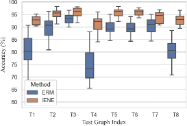
Figure 2: Results on Cora under OOD. Compared to ERM, IENE significantly improves the accuracy and stability of GNN.

(c) Efficiency Comparison. Table 3 illustrates the efficiency comparison of the three variants of IENE, EERM, and TIVA on the Cora dataset. The backbone network for experiments is GCN, and the hyperparameters for these frameworks are unified. Note that, due to the two-stage training strategy employed in both IENE and TIVA, the runtime for every 100 epochs in the table represents the average time for both stages. The time cost of IENE-r is mainly determined by the bi-level optimization between the classifiers in discrete environments and the shared classifier, along with the alternating learning of the two representation extractors. The time cost of IENE-e primarily depends on the bi-level optimization between the view augmentation component and the invariant learner. Compared to the retraining method EERM, IENE-e adopts a similar training pattern but exhibits higher efficiency. IENE-r and TIVA share a similar training pattern, resulting in a small efficiency gap between them. Furthermore, IENE-re combines the two proposed methods, achieving superior OOD generalization performance without incurring significant additional memory overhead. Note that both IENE-e and IENE-re include the time and memory occupied by the pre-training phase of IENE-r.

5 Conclusion

In this paper, we propose a novel method, IENE, to achieve OOD generalization of GNNs from the perspective of invariant learning. First, we present a fully data-driven environmental inference method that extracts environmental representation and partitions environments with a disentangled information bottleneck framework, simultaneously discovers invariance in features. Besides, we analyze the characteristics of invariance on graph-structured data and design a augmentation-based method for environmental extrapolation, generating a series of environmental views to learn invariance in the structure of graphs. Additionally, we integrate environmental identification, environmental extrapolation techniques, and an invariance learning framework to discover invariant patterns on graph. In practice, we have implemented conceptual methods specifically, and for stability, we conduct invariant learning in a bilevel optimization manner. We theoretically and experimentally demonstrate that IENE can automatically learn invariance from input graphs, achieving competitive generalization performance on OOD datasets. The evaluation also validated our theoretical analysis. In future work, We will enhance the scalability of IENE to adapt to large-scale graphs and apply the method to specific GNN-based real-world scenarios to address the OOD problem.

Appendix

Appendix A Learning Algorithm

IENE-re combines IENE-r and IENE-e, and its objective function is given by Eqn. (LABEL:equation11).

$$\min_{c,\Phi}\max_{w,c_{1},...,c_{K}}\mathcal{R}(c,\Phi)+\lambda\cdot{\textstyle\sum_{k=1}^{K}}\left[\mathcal{R}^{k}_{\rho_{u,w}}(c,\Phi)-\mathcal{R}^{k}_{\rho_{u,w}}(c_{k},\Phi)\right]+\mathcal{L}(\hat{G}^{(k)},Y)+\beta\cdot\mathbb{V}(\mathcal{L}(\hat{G}^{(k)},Y))$$ (11)

Detailed variable explanations can be found in Eqn. (LABEL:equation9) and (LABEL:equation10). Since the Eqn. (LABEL:equation11) involve a max-min objective, it is complex and challenging to optimize directly. Therefore, in practice, we can complete the learning of different components in stages. In general, during the implementation process, we can follow a two-stage training approach to optimize the model. The complete algorithm is provided in algorithm 1.

Algorithm 1 IENE-re

  Input: invariant feature extractor $\Phi$, invariant label classifier $c$, environmental feature extractor $u$, environmental index classifier $w$, environmental label classifier $c_{1},...,c_{K}$, feature reconstructor $d$, Input graph $G$ and target $Y$.

  1.Stage-one: Annealing Iteration

  for each annealing iteration do

     for each disentanglement iteration do

        Train $u,d$ by minimize the constraint part of Eqn. (LABEL:equation9) with fixed $\Phi$.

     end for

     Train $c_{1},...,c_{K}$ by minimizing the ERM loss ${\textstyle\sum_{k=1}^{K}}\mathcal{R}(c_{k},\Phi)$ with fixed $\Phi$.

     Train $\Phi,c$, by minimize the Eqn. (5) with fixed $u,w$ and $c_{1},...,c_{K}$.

     Train $w$ by maximize the Eqn. (5) with fixed $u,\Phi,c$ and $c_{1},...,c_{K}$.

  end for

  2.Stage-two: Invariant Learning Iteration

  for each training iteration do

     for each structural intervention iteration do

        Train $\hat{G}_{v}^{(1)},...,\hat{G}_{v}^{(K)}$ by minimize the Eqn. (6) with fixed $u,w$.

     end for

     Train $\Phi,c$ by minimize the Eqn. (LABEL:equation11) with fixed $u,w$ and $c_{1},...,c_{K}$.

  end for

Appendix B Conceptual Analysis and Discussion

B.1 Auxiliary Information for Identifying the Environment

$X_{v_{i}}$ provides no benefits for environment identification and may even introduce additional noise, while $X_{v_{s}}$ and $X_{v_{ir}}$ play an important role in inferring the environment. According to the assumption, the probability distribution $P(Y|X_{v_{s}})$ varies across different environments $e\in\varepsilon$, while $P(Y|X_{v_{i}})$ remains invariant, i.e., $P(Y|X_{v_{i}},e)=P(Y|X_{v_{i}},e^{\prime})$.

Here, we consider two cases of $X_{v_{i}}$.

The first case corresponds to Figure 1(a)(b), where the nodes in the figure are generated based on a Structural Causal Model (SCM) with a directed acyclic graph. Assuming the Markov property and other underlying assumptions hold, in both causal graphs, we have Condition $X_{i}\bot e$, indicating that $X_{i}$ manifests as noise relative to the environment $e$.

The second case corresponds to Figure 1(c). Clearly, in this causal graph, $X_{i}\not\!\bot\ e$, due to $e\to X_{2}$. While $X_{2}$ may contribute to environmental inference, it is essential to emphasize that within the framework of invariant learning, the purpose of environment partitioning is to maximize the differences in $P(Y|X_{v_{s}})$ across different partitions, providing an invariant penalty. This aims to prevent the invariant representation learner $\Phi$ from extracting spurious features $X_{v_{s}}$ from the input graph. If we use $X_{2}$ as the input for environmental prediction, where different values $X_{2}^{(1)}\neq X_{2}^{(2)}$ of $X_{2}$ correspond to inferred environments $e^{(1)}$ and $e^{(2)}$, we have $P(Y|X_{2},e^{(1)})\neq P(Y|X_{2},e^{(2)})$. Consequently, the subset of invariant features $X_{2}\in X_{i}$ is considered by the invariant learner as spurious, hindering the learning of invariant features with similar properties.

Therefore, $X_{i}$ should not be used for predicting the environment in any case.

According to the previous assumptions, $P(Y|X_{v_{s}},e)\neq P(Y|Y|X_{v_{s}},e^{\prime})$. In the causal graph, the relationship between $X_{v_{s}}$ and the environment $e$ can be considered as a direct or latent causal relationship. Therefore, it is reasonable to use $X_{v_{s}}$ as a basis for predicting the environment. Literature [43] assumes that features $X_{v_{ir}}$ unrelated to the target $Y$ can be used to predict the environment, such as background factors like time or location. While this assumption is possible, it may not always hold. Thus, we believe that both $X_{v_{s}}$ and $X_{v_{ir}}$ play important roles in environmental reasoning.

B.2 Adaptation to Structural Environment Changes

Training an invariant model on static graph data may face challenges in adapting to changes in the structural environment. In data with independent samples, Method in 3.1 theoretically excels at identifying invariant features. However, in graph-structured data, nodes’ representations are not independent of those of their neighbors. This characteristic leads the learner $\Phi$ (composed of some GNN layers, to learn high-quality information from graph-organized data), to inevitably aggregate the invariant features of the neighbors when learning the invariant representation $h_{v_{i}}$ of node $v$. When structural changes occur, this aggregation may significantly impact the learned invariant representation, resulting in failures in downstream tasks. In other words, training $\Phi$ using Eqn. (5) can only guarantee the identification of invariant features on graphs with similar structural properties. For a single graph, Method in 3.1 can only learn to identify invariant features under a static context, and it is not invariant to changes in structural properties. Therefore, we extend the method to environment extrapolation, conducting dynamic invariant learning through environment augmentation. This is verified in the ablation experiments in Appendix D.5.

B.3 The Limitations of V-REx

In certain cases of node classification, V-REx [22] may struggle to impose a significant penalty for dissimilarity. Here, we illustrate this issue with a simple example. We consider two views, $G^{(1)}$ and $G^{(2)}$, from different environments. When $\mathbb{E}_{v}l(f(G_{v}^{(1)}),y_{v})\approx\mathbb{E}_{v}l(f(G_{v}^{(2)}),y_{v})$, V-REx $\mathbb{V}_{k}(\mathcal{L}((G^{(1)}),Y))\approx 0$, but for a node $v\in V$, there may be a significant difference between $l(f(G_{v}^{(1)}),y_{v})$ and $l(f(G_{v}^{(2)}),y_{v})$, indicating that graph-level V-REx fails to capture node-level differences. In more extreme cases, where nodes correctly classified in one view are complementary to those in the other view, they may still exhibit similar loss values at the graph level (However, from the perspective of node-wise environment, these two views are vastly different). Therefore, V-REx perceives their performance as similar and may not impose a significant penalty. NV-REx, on the other hand, is capable of providing a positive penalty based on the differences of each node in different environments, accumulating them to better penalize the learned features for their dissimilarity across environments, compelling the learner to acquire invariant features.

B.4 Feature Learning Preserves Invariance

In IENE, the invariant representation $h_{v_{i}}=\Phi(G_{v})$ is capable of preserving observations of $X_{v_{i}}$. In this section, following [2, 36, 29], we will demonstrate that IENE can learn invariant features given a scrambled observation in a linear form. Specifically, we consider the same data generation process as [2]:

$$Y^{e}=X_{i}^{e}\cdot\beta+\epsilon_{i},X_{i}^{e}\perp\epsilon_{i},\mathbb{E}(\epsilon_{i})=0,X^{e}=W\cdot[X_{i}^{e},X_{s}^{e}]$$ (12)

where $\beta\in\mathbb{R}^{d_{i}}$ and $W\in\mathbb{R}^{d\times(d_{i}+d_{s})}$. We assume the existence of $\widetilde{W}\in\mathbb{R}^{d_{i}\times d}$ such that $\widetilde{W}(W[x_{i};x_{s}])=x_{i}$ for all $x_{i}$ and $x_{s}$. Both the feature extractor and predictor adopt a linear form, that is, $\Phi$ takes values in $\mathbb{R}^{d\times d}$ and $x_{i}$ takes values in $\mathbb{R}^{d}$. The prediction for $X$ is $\omega\circ\Phi(X)=(\Phi X)^{T}\omega$.

In this case, a major challenge lies in describing the impact of an invariant or spurious feature in a quantitative manner: the feature extractor $\Phi$ can capture arbitrary small portions of spurious information. Following [2, 36, 29], we consider a constrained form of problem 5 for theoretical analysis:

$$\min_{c,\Phi}\mathcal{R}(c,\Phi),s.t.\max_{u,w,c_{k}}{\textstyle\sum_{k=1}^{K}}[\mathcal{R}^{k}_{\rho_{u,w}}(c,\Phi)-\mathcal{R}^{k}_{\rho_{u,w}}(c_{k},\Phi)]$$ (13)

Similar to condition 1 and condition 2, auxiliary information should also provide sufficient information so that the inferred environment can be diverse enough while maintaining latent invariance. This aligns with existing conditions for identifiability in linear cases [36, 29]. In this paper, we leverage such a condition, $lineargeneralpositioncondition$, from [2]. For our analysis, we use squared error as the loss function and consider that $\rho(\cdot)$ partitions the environments in a challenging way, where each data sample is precisely assigned to one environment. We use $L(\cdot|\cdot)$ to denote the optimal expected risk. We also assume that environments are non-degenerate, meaning each inferred environment contains some data samples; otherwise, we can simply remove such environments. The identifiability results for the linear case are as follows.

Proposition 1.

Suppose $H(\cdot|\cdot)$ in condition 1 is replaced by $L(\cdot|\cdot)$. Assume the existence of $\rho(\cdot)$ such that the generated environments, denoted as $\{X^{k}\}_{k=1}^{K}$, are in linear generic position of degree $r$. For example, for some $r\in\mathbb{N}$, there exists $K>d-r+d/r$, and for any non-zero $x\in\mathbb{R}^{d}:dim(span(\{\mathbb{E}_{X^{k}}[X^{k}X^{k^{T}}]x-\mathbb{E}_{X^{k},\epsilon_{i}}[X^{k}]\epsilon_{i}\}_{k}))>d-r$. If the rank of $\Phi\in\mathbb{R}^{d\times d}$, $r>0$, then Eqn. (LABEL:equation13) will yield the expected invariant predictor.

Proof. Step 1: No spurious feature will be learned. Given a partition $\{X^{k}\}_{k=1}^{K}$ in linear generic position of degree $r$, theorem 9 in [2] demonstrates that for any $k$, $\Phi$, and $\omega$ satisfying the normal equations $\Phi\mathbb{E}_{X^{k}}[X^{k}X^{k^{T}}]\Phi^{T}\omega=\Phi\mathbb{E}_{X^{k},Y^{k}}[X^{k}Y^{k}]$, it holds if and only if $\Phi$ leads to the desired invariant predictor $\Phi^{T}\omega=\widetilde{W}^{T}\beta$. Therefore, we only need to prove that our solution satisfies the same normal equations. Let $\Phi^{\prime}$ and $\omega^{\prime}$ denote the solution to Eqn. (LABEL:equation13). According to the constraints and the general linear position condition, we know that there exists a partition $\{X^{k}\}_{k=1}^{K}$ in general linear position of degree $r$, where $\mathcal{R}^{k}(\omega^{\prime},\Phi^{\prime})=\mathcal{R}^{k}(\omega_{k},\Phi^{\prime})$. Note that $\omega_{k}$ only minimizes the mean squared error in the $k$-th environment, so it must satisfy the normal equation $\Phi^{\prime}\mathbb{E}_{X^{k}}[X^{k}X^{k^{T}}]\Phi^{\prime T}\omega=\Phi^{\prime}\mathbb{E}_{X^{k},Y^{k}}[X^{k}Y^{k}]$. As $\omega^{\prime}$ achieves the same minimal mean squared error in the $k$-th environment, $\omega^{\prime}$ must also satisfy the normal equations. Therefore, the invariant representation contains no spurious information, $X\Phi=[SX_{i};0_{d_{s}}]$, where $S\in\mathbb{R}^{d_{i}\times d_{i}}$ is a reversible matrix, and $0_{d_{s}}$ represents $d_{s}$- dimensional vectors with all elements being zero.

Step 2: The representation does not discard any invariance information. With $H(\cdot|\cdot)$ replaced by $L(\cdot|\cdot)$ in condition 1, we have $L(Y|X_{i})-L(Y|X_{i},w(u(G)))=0$. Then $X\Phi$ will satisfy the constraints of Eqn. (LABEL:equation13). Note that the obtained loss for $X\Phi$ is minimized when only using invariant feature information.

B.5 More Discussions on Identifiable Invariance

IENE may inevitably overlook a small portion of invariant features, but this does not affect our ability to identify more influential and stable invariant features for predicting $Y$. Considering the case in Figure 1(c), $X_{2}$, a subset of invariant features may be mistaken as spurious features due to changes in the environment, leading to $P(Y|X_{2},e^{(1)})\neq P(Y|X_{2},e^{(2)})$. However, we can adjust the learning extent of the invariant learner for features like $X_{2}$ by controlling the trade-off between ERM loss and invariant penalty. When the invariant penalty dominates, the invariant learner tends to reject learning $X_{2}$ (while rejecting all spurious features, but sacrificing information in $X_{2}$ that is helpful for predicting $Y$); when the ERM loss dominates, it tends to learn from $X_{2}$ because it contains causal features for $Y$ (retaining most of the information helpful for predicting $Y$ in $X_{2}$, but possibly learning some spurious features $x_{s}\in X_{4}$). Invariant features $X_{2}^{s}\subseteq X_{2}$, which play a more critical role in predicting $Y$, are not overlooked, as this would significantly increase the ERM loss and dominate the training, prompting the relearning of invariant features from $X_{2}^{s}$.

B.6 Prerequisites and Assumptions

In IENE, the invariant representation $h_{v_{i}}=\Phi(G_{v})$ not only preserves observations of the original invariant features $X_{v_{i}}$ in the raw data but also captures new invariances, as demonstrated in Appendix B.4. Based on this, we can relax the assumptions about the data.

Assumption 1.

There exist invariant features $X_{v_{i}}$ in the original features $X_{v}$ of $G_{v}$, or $h_{v_{i}}$ obtained by some linear transformation $\Phi$ on the original features $X_{v}$ satisfies the invariance property, i.e., Property 1.

Property 1.

(Invariance Property): In causal graph, under any intervention at any node (except $Y$ itself), $P(Y|X_{i})$ or $P(Y|h_{i})$ remains invariant.

For simplicity, in the subsequent descriptions, we use $X_{i}$ to refer to $X_{i}$ or $h_{i}$, and $X_{s}$ to refer to $X_{s}$ or $h_{s}$, as they share similar properties. We then introduce the following assumptions, which are similar to assumptions 1-3 in the literature [29, 43].

Assumption 2.

For any given learning function $\Phi$ and any constant $\epsilon>0$, there exists $c\in F$, such that $\mathbb{E}[\mathcal{L}(c(\Phi(G)),Y)]\leq H(Y|\Phi(G))+\epsilon$.

Assumption 3.

If a feature violates the invariance constraint, adding another feature will not eliminate the penalty, i.e., there exists a constant $\delta>0$ such that for spurious feature $X_{1}\subset X_{s}$ and any feature $X_{2}\subset X$, we have $H(Y|X_{1},X_{2})-H(Y|w(u(G)),X_{1},X_{2})\geq\delta(H(Y|X_{1})-H(Y|w(u(G)),X_{1}))$.

Assumption 4.

Let $X_{i}^{s}$ represent any appropriate subset of invariant features, i.e., $X_{i}^{s}\subsetneq X_{i}$, we have $H(Y|X_{i})\leq H(Y|X_{i}^{s})-\gamma$, where $\gamma$ is a constant and $\gamma>0$.

Assumption 2 is a common assumption, requiring that the function space is rich enough. So, given $\Phi$, there exists $c\in F$ that can fit $P(Y|\Phi(G))$ well. The purpose of Assumption 3 is to ensure sufficient positive penalty when spurious features are included. Assumption 4 indicates that any set of features contains some information useful for predicting $Y$. Otherwise, we could simply remove such a class of irrelevant features as they do not impact predictions.

As discussed in Section 3.3.1, if $u(\cdot)$, $w(\cdot)$, $\Phi(\cdot)$, and $c(\cdot)$ satisfy condition 1, 2, and 3, Eqn. (5) and (LABEL:equation8) can be proven to learn invariant features, and the downstream classifier exhibits the same and optimal performance across different environments.

Condition 1.

(Invariance Condition): Given the invariant feature $X_{i}$ and any environment index classifier $w(\cdot)$, it holds that $H(Y|X_{i},w(u(G)))=H(Y|X_{i})$.

Condition 2.

(Non-Invariance Discrimination Condition): For any feature $X_{s}^{s}\in X_{s}$, there exists an environment index classifier $w(\cdot)$ and a constant $C>0$, such that $H(Y|X_{s}^{s})-H(Y|X_{s}^{s},w(u(G)))\geq C$.

Condition 3.

(Sufficiency Condition): For the invariant feature encoder $\Phi(\cdot)$ and classifier $c(\cdot)$, $Y=c(\Phi(G))+n$, where $n$ is independent noise.

Condition 1 requires that the invariant feature $X_{i}$ caused by $w(u(G))$ should remain invariant for any environment partition. Otherwise, if there is a partition where an invariant feature changes, that feature will result in a positive penalty. Condition 2 implies that, for each spurious feature, there is at least one partition where this feature is non-invariant in a split environment. If a spurious feature does not receive any invariance penalty in all possible environment partitions, we can never distinguish it from a truly invariant feature.

Then, the next assumption will serve as the foundation for our environmental extrapolation approach.

Assumption 5.

(Environmental Heterogeneity): For $\Phi$, $u$, and $w$ satisfying conditions 1 and 2, there exists a function mapping $m$ such that $G^{(e)}=m(G,n^{(e)})$. And $P(Y|X^{k}_{s},w(u(G)))$ can arbitrarily vary across different environments.

Are these assumptions difficult to hold? These assumptions are explicitly or implicitly required in a series of works such as IRM, ZIN, TIVA, and VREx. Therefore, we believe that assumptions 1-4 used in this paper are nearly unavoidable in the current framework of invariant learning based on environmental partitioning. And assumption 5 is also a common assumption in graph invariant learning works such as EERM and DIR. We believe that the success of these works indicates that these assumptions are generally easy to hold in reality.

Appendix C Proofs

C.1 Proof of Theorem 1

To prove Theorem 1, we can replace $X_{v}$ and $X_{s}$ with $h_{v_{i}}$ and $h_{v_{s}}$ in the proof of Theorem 2 as presented by [29].

C.2 Proof of Theorem 2

Lemma 1.

Condition 1 (Invariance) can be equivalently expressed as: $I(Y;w(u(G))|h_{i})=0$, and Condition 3 (Sufficiency) can be equivalently represented as: $I(Y;h_{i})$ is maximized.

Proof. For invariance, we can easily derive equivalent expressions for the given facts.

$$I(Y;w(u(G))|h_{i})=D_{KL}(P(Y,w(u(G))|h_{i})||P(Y|h_{i})P(w(u(G))|h_{i}))$$ (14)

$$=D_{KL}(P(Y|w(u(G)),h_{i})||P(Y|h_{i}))]$$

For sufficiency, we first prove that if $Y=c^{*}(h_{i})+n$ is satisfied, then $h_{i}=argmax_{h}I(Y;h)$ will also be satisfied simultaneously. Let $h^{\prime}=argmax_{h}I(Y;h),h_{i}\in supp(h_{i})$, and we prove this by showing that $I(Y;h^{\prime})\leq I(Y;h_{i})$. There exists a random variable $\overline{h}_{i}$ that is independent of $h_{i}$ and $h^{\prime}$ can be expressed as $h^{\prime}=m(h_{i},\overline{h}_{i})$, where $m$ is a mapping function. Then, we can derive the following:

$$I(Y;h^{\prime})=I(Y;m(h_{i},\overline{h}_{i}))\leq I(Y;h_{i},\overline{h}_{i})=I(c^{*}(h_{i})+n;h_{i},\overline{h}_{i})=I(c^{*}(h_{i});h_{i})=I(Y;h_{i})$$

Due to $h^{\prime}=argmax_{h}I(Y;h)$ and $I(Y;h^{\prime})\leq I(Y;h_{i})$, we have $h^{\prime}=h_{i}=argmax_{h}I(Y;h)$ Next, we prove that for $(h_{i},Y)$, if $h_{i}=argmax_{h}I(Y;h)$ is satisfied, then $Y=c^{*}(h_{i})+n$ will also be satisfied. We will prove this by contradiction. Suppose $Y\neq c^{*}(h_{i})+n$ and $Y=c^{*}(h^{\prime})+n$ hold, where $h^{\prime}\neq h_{i}$. Then, based on sufficiency, we have $I(c^{*}(h^{\prime});h_{i})\leq I(c^{*}(h^{\prime});h^{\prime})$. Consequently, $h^{\prime}=argmax_{h}I(Y;h)=h_{i}$, which contradicts the given conditions. Therefore, $Y=c^{*}(h_{i})+n$.

Lemma 1 has been proven.

For Lemma 1, we know that 1) the node representation $h_{v_{i}}$ (given by the GNN encoder $h_{v_{i}}=\Phi(G_{v})$) satisfies the invariant condition, i.e., $P(y|h_{v_{i}},e_{v})=P(y|h_{v_{i}})$ if and only if $I(y;e_{v}|h_{v_{i}})=0$, and 2) the node representation $h_{v_{i}}$ satisfies the necessary and sufficient condition, i.e., $Y=c^{*}(h_{v_{i}})+n$ if and only if $h_{v_{i}}=argmax_{h_{v}}I(y;h_{v})$.

We denote the GNN encoder that satisfies condition 1 (Invariance condition) and condition 3 (Sufficiency condition) as $\Phi^{*}$, and we represent the corresponding predictor model as $f^{*}(\cdot)=c^{*}(\Phi^{*}(\cdot))$. Let $z$ be an instance of $h_{v_{i}}$. According to assumption 5, we know that there exists a random variable $\overline{z}$ such that $G_{v}=m(z,\overline{z})$ and $P(y|\overline{z},e_{v})$ can vary arbitrarily across different environments. Based on this, for any given distribution $P_{e}(y,z,\overline{z})$ over environment $e$, there exists an environment $e^{\prime}$ that satisfies the distribution $P_{e^{\prime}}(y,z,\overline{z})$ such that

$$P_{e^{\prime}}(y,z,\overline{z})=P_{e}(y,z)P_{e^{\prime}}(\overline{z})]$$ (15)

Then, following the reasoning line of Theorem 2 in [49], we can prove that for any function $f=c\circ\Phi$ and environment $e$, there exists an environment $e^{\prime}$ such that

$$\scalebox{0.8}{$\frac{1}{|V|}\sum_{v\in V}\mathbb{E}_{G_{v}\sim p_{e^{\prime}}(\boldsymbol{G_{v}})}\mathbb{E}_{y_{v}\sim p_{e^{\prime}}(\boldsymbol{y}|\boldsymbol{G_{v}}=G_{v})}[l(f(G_{v}),y_{v})]\geq\frac{1}{|V|}\sum_{v\in V}\mathbb{E}_{G_{v}\sim p_{e}(\boldsymbol{G_{v}})}\mathbb{E}_{y_{v}\sim p_{e}(\boldsymbol{y}|\boldsymbol{G_{v}}=G_{v})}[l(f^{*}(G_{v}),y_{v})]$}$$

Specifically, we have

$$\scalebox{0.8}{$\frac{1}{|V|}\sum_{v\in V}\mathbb{E}_{G_{v}\sim p_{e^{\prime}}(\boldsymbol{G_{v}})}\mathbb{E}_{(y_{v},z_{v},\overline{z}_{v})\sim p_{e^{\prime}}(\boldsymbol{y,z,\overline{z}}|\boldsymbol{G_{v}}=G_{v})}[l(c(z_{v},\overline{z}_{v}),y_{v})]$}$$

$$\scalebox{0.8}{$=\frac{1}{|V^{\prime}|}\sum_{v^{\prime}\in V^{\prime}}\mathbb{E}_{G^{\prime}_{v}\sim p_{e^{\prime}}(\boldsymbol{G_{v}})}\mathbb{E}_{(\overline{z}_{v^{\prime}})\sim p_{e^{\prime}}(\boldsymbol{\overline{z}}|\boldsymbol{G_{v}}=G_{v})}[\frac{1}{|V|}\sum_{v\in V}\mathbb{E}_{G_{v}\sim p_{e}(\boldsymbol{G_{v}})}\mathbb{E}_{(y_{v},z_{v})\sim p_{e}(\boldsymbol{y,z}|\boldsymbol{G_{v}}=G_{v})}[l(c(z_{v},\overline{z}_{v^{\prime}}),y_{v})]$}$$

$$\scalebox{0.8}{$\geq\frac{1}{|V^{\prime}|}\sum_{v^{\prime}\in V^{\prime}}\mathbb{E}_{G^{\prime}_{v}\sim p_{e^{\prime}}(\boldsymbol{G_{v}})}\mathbb{E}_{(\overline{z}_{v^{\prime}})\sim p_{e^{\prime}}(\boldsymbol{\overline{z}}|\boldsymbol{G_{v}}=G_{v})}[\frac{1}{|V|}\sum_{v\in V}\mathbb{E}_{G_{v}\sim p_{e}(\boldsymbol{G_{v}})}\mathbb{E}_{(y_{v},z_{v})\sim p_{e}(\boldsymbol{y,z}|\boldsymbol{G_{v}}=G_{v})}[l(c^{*}(z_{v},\overline{z}_{v^{\prime}}),y_{v})]$}$$

$$\scalebox{0.8}{$=\frac{1}{|V^{\prime}|}\sum_{v^{\prime}\in V^{\prime}}\mathbb{E}_{G^{\prime}_{v}\sim p_{e^{\prime}}(\boldsymbol{G_{v}})}\mathbb{E}_{(\overline{z}_{v^{\prime}})\sim p_{e^{\prime}}(\boldsymbol{\overline{z}}|\boldsymbol{G_{v}}=G_{v})}[\frac{1}{|V|}\sum_{v\in V}\mathbb{E}_{G_{v}\sim p_{e}(\boldsymbol{G_{v}})}\mathbb{E}_{(y_{v},z_{v})\sim p_{e}(\boldsymbol{y,z}|\boldsymbol{G_{v}}=G_{v})}[l(c^{*}(z_{v}),y_{v})]$}$$

$$\scalebox{0.8}{$=\frac{1}{|V|}\sum_{v\in V}\mathbb{E}_{G_{v}\sim p_{e}(\boldsymbol{G_{v}})}\mathbb{E}_{y_{v}\sim p_{e}(\boldsymbol{y}|\boldsymbol{G_{v}}=G_{v})}[l(f^{*}(G_{v}),y_{v})]]$}$$

The first equality is given by Eqn. (LABEL:equation15), and the second/third steps are due to the sufficiency condition (condition 3) of $\Phi^{*}$. Therefore, a function $f^{*}$ that satisfies both condition 1 and condition 3 will have optimal performance across all environments.

C.3 NV-REx

Here, we will demonstrate that our invariant regularizer NV-REx, provides a tighter upper bound compared to V-REx.

$Proof$. First, from a node-level perspective, let’s redefine the KL distance as:

$$D_{KL}(p_{e}(\boldsymbol{y|G_{v}})||q(\boldsymbol{y|G_{v}})):=\frac{1}{|V|}\sum_{v\in V}\mathbb{E}_{G_{v}\sim p_{e}(\boldsymbol{G_{v}})}\mathbb{E}_{y_{v}\sim p_{e}(\boldsymbol{y}|\boldsymbol{G_{v}}=G_{v})}[log\frac{p_{e}(\boldsymbol{y}=y_{v}|\boldsymbol{G_{v}}=G_{v})}{q(\boldsymbol{y}=y_{v}|\boldsymbol{G_{v}}=G_{v})}]$$ (16)

We utilize $D_{KL}(q(\boldsymbol{y|z})||\mathbb{E}_{\boldsymbol{e}}[q(\boldsymbol{y|z})])$ to measure the generalization error,

$$D_{KL}(q(\boldsymbol{y|z})||\mathbb{E}_{\boldsymbol{e}}[q(\boldsymbol{y|z})])$$

$$\scalebox{0.8}{$\frac{1}{|V|}\sum_{v\in V}\mathbb{E}_{\boldsymbol{e}}\mathbb{E}_{G\sim p_{e}(\boldsymbol{G})}\mathbb{E}_{y_{v}\sim p_{e}(\boldsymbol{y|G_{v}}=G_{v})}\mathbb{E}_{z_{v}\sim p_{e}(\boldsymbol{z|G_{v}}=G_{v})}[log\frac{q(\boldsymbol{y}=y_{v}|\boldsymbol{z}=z_{v})}{\mathbb{E}_{\boldsymbol{e}}[q(\boldsymbol{y}=y_{v}|\boldsymbol{z}=z_{v})]}]$}$$

$$\scalebox{0.8}{$=\frac{1}{|V|}\sum_{v\in V}\mathbb{E}_{\boldsymbol{e}}\mathbb{E}_{G\sim p_{e}(\boldsymbol{G})}\mathbb{E}_{y_{v}\sim p_{e}(\boldsymbol{y|G_{v}}=G_{v})}\mathbb{E}_{z_{v}\sim p_{e}(\boldsymbol{z|G_{v}}=G_{v})}[log\ q(\boldsymbol{y}=y_{v}|\boldsymbol{z}=z_{v})-log\mathbb{E}_{\boldsymbol{e}}\left[q(\boldsymbol{y}=y_{v}|\boldsymbol{z}=z_{v})\right]]$}$$

$$\scalebox{0.8}{$\leq\frac{1}{|V|}\sum_{v\in V}\mathbb{E}_{\boldsymbol{e}}\mathbb{E}_{G\sim p_{e}(\boldsymbol{G})}\mathbb{E}_{y_{v}\sim p_{e}(\boldsymbol{y|G_{v}}=G_{v})}\mathbb{E}_{z_{v}\sim p_{e}(\boldsymbol{z|G_{v}}=G_{v})}[log\ q(\boldsymbol{y}=y_{v}|\boldsymbol{z}=z_{v})-\mathbb{E}_{\boldsymbol{e}}\left[log\ q(\boldsymbol{y}=y_{v}|\boldsymbol{z}=z_{v})\right]]$}$$

Using Jensen Inequality, we can also obtain an upper bound for $D_{KL}(q(\boldsymbol{y|z})||\mathbb{E}_{\boldsymbol{e}}[q(\boldsymbol{y|z})])$ as

$${\textstyle\sum_{v\in V}}\mathbb{E}_{\boldsymbol{e}}|l(f(G_{v}),y_{v})-\mathbb{E}_{\boldsymbol{e}}[l(f(G_{v}),y_{v})]|$$ (17)

We optimize its squared form, denoted as $\mathbb{V}_{node-wise}={\textstyle\sum_{v\in V}}\mathbb{E}_{\boldsymbol{e}}[l(f(G_{v}),y_{v})-\mathbb{E}_{\boldsymbol{e}}[l(f(G_{v}),y_{v})]]^{2}$. Similarly, utilizing Jensen Inequality, we have:

$$\mathbb{V}_{node-wise}=$$

$$\scalebox{0.8}{$\frac{1}{|V|}\sum_{v\in V}\mathbb{E}_{\boldsymbol{e}}\mathbb{E}_{G\sim p_{e}(\boldsymbol{G})}\mathbb{E}_{y_{v}\sim p_{e}(\boldsymbol{y|G_{v}}=G_{v})}\mathbb{E}_{z_{v}\sim p_{e}(\boldsymbol{z|G_{v}}=G_{v})}[log\ q(\boldsymbol{y}=y_{v}|\boldsymbol{z}=z_{v})-\mathbb{E}_{\boldsymbol{e}}\left[log\ q(\boldsymbol{y}=y_{v}|\boldsymbol{z}=z_{v})\right]]$}$$

$$\scalebox{0.8}{$\leq\mathbb{E}_{\boldsymbol{e}}\frac{1}{|V|}\sum_{v\in V}\mathbb{E}_{G\sim p_{e}(\boldsymbol{G})}\mathbb{E}_{y_{v}\sim p_{e}(\boldsymbol{y|G_{v}}=G_{v})}\mathbb{E}_{z_{v}\sim p_{e}(\boldsymbol{z|G_{v}}=G_{v})}[log\ q(\boldsymbol{y}=y_{v}|\boldsymbol{z}=z_{v})-\mathbb{E}_{\boldsymbol{e}}\left[log\ q(\boldsymbol{y}=y_{v}|\boldsymbol{z}=z_{v})\right]]$}$$

$$=\mathbb{V}_{graph-wise}$$

Therefore, optimizing NV-REx ($\mathbb{V}_{node-wise}$) compared to V-REx ($\mathbb{V}_{graph-wise}$) allows the generalization error to converge to a tighter upper bound.

Appendix D Ablation Experiments

D.1 Supplementary Table

Table 3: Efficiency Comparison. IENE-re achieves superior OOD generalization performance and demonstrates better time and space efficiency compared to EERM. Experiments were conducted on Nvidia A40 (48G).

	Running Time (s/100 epochs)				Total GPU Memory(GB)
	Cora	Amz-Photo	Elliptic	OGB-Arxiv	Cora	Amz-Photo	Elliptic	OGB-Arxiv
TIVA	7	13	31	47	2.23	3.71	4.02	5.49
IENE-r	9	21	45	62	2.41	3.97	4.76	8.69
EERM	30	174	280	440	4.19	18.79	19.78	33.64
IENE-e	13	62	130	311	3.02	8.27	10.81	25.24
IENE-re	14	66	137	328	3.03	8.48	10.99	25.36

D.2 Selection of Auxiliary Information

To assess the influence of auxiliary information on performance, we performed ablation studies on the synthetic dataset described in Section 4. We specifically employed environmental representation $h_{v_{e}}$, irrelevant features ${X_{ir}}$, and random noise $n$ as auxiliary information for environmental partitioning. The informative content of each auxiliary information was evaluated by measuring the average accuracy. For identifying irrelevant features ${X_{ir}}$, we adopted the methodology proposed by TIVA [43], while standard Gaussian noise was utilized for the random noise $n$. The experimental settings were consistent with those described in Section 4.2. The final experimental results are presented in Table 4.

Table 4: The ablation study reults on different selection of auxiliary information.

	$h_{v_{e}}$	$X_{ir}$	$n$
Cora	95.58$\pm$ 2.07	94.33$\pm$2.18	91.41$\pm$3.59
Amz-Photo	96.40 $\pm$1.80	95.45 $\pm$2.60	91.78 $\pm$1.73

Based on the results of the ablation study, we observed that using $h_{v_{e}}$ for environmental recognition yielded the best performance, while using $X_{ir}$ resulted in suboptimal performance. This can be attributed to the fact that $h_{v_{e}}$ not only learns from $X_{ir}$ but also incorporates rich spurious feature information that is causally related to the environment. These spurious features play a direct and key role in environmental partitioning. Additionally, our ablation study indicates that the model cannot utilize random noise as auxiliary information since it does not contain any information about $X$, thus it is unable to assist in distinguishing the spurious features. It is worth noting that when no useful component is found in the auxiliary information, the model would degrade to ERM (Empirical Risk Minimization).

D.3 V-REx and NV-REx

According to Appendix C.3, we have theoretically proven that the node-level variance (NV-REx) possesses a tighter upper bound compared to the graph-level variance (V-REx). Here, we further validate their performance as invariant penalties. We employ GCN as the backbone network and train the models using the IENE-re method on six datasets. The experimental settings are identical, except for the invariant penalty. The results are presented in Table 5.

Table 5: The ablation study reults on different selection of variance penalty.

	V-REx	NV-REx
Cora	94.71$\pm$ 2.29	95.58$\pm$2.07
Amz-Photo	95.48 $\pm$1.32	96.40 $\pm$1.80
Twitch-E	59.57 $\pm$2.51	61.87 $\pm$1.43
FB-100	52.46 $\pm$1.69	53.73 $\pm$2.65
Elliptic	66.85 $\pm$1.54	67.90 $\pm$3.31
OGB-Arxiv	44.19 $\pm$0.90	44.85 $\pm$0.33

As shown in Table 5, NV-REx demonstrates better performance on all datasets. This indicates that in the task of node classification on graphs under out-of-distribution (OOD) settings, NV-REx achieves better performance as it can identify a greater amount of environmental variations.

D.4 Method of Environment Extrapolation

We explored different graph augmentation methods and validated the effectiveness of using IENE-re for extrapolating beyond known environments. It is important to note that EERM and FLOOD generate augmented views by randomly adding or removing edges. We will compare the following methods for generating environment views: a method based on random edge dropout [47], a method based on gradient perturbation of edges [53], and EERM [49]. Each method has the same edge adjustment budget. It is worth emphasizing that these methods only differ in their view generation approaches, while the training framework remains the same as IENE-re. The results are presented in Table 6.

Table 6: The ablation study results on different methods of environment extrapolation.

	Cora	Amaz-Photo
Random	91.43$\pm$ 3.96	93.17$\pm$1.63
Grad-based	93.49 $\pm$2.50	95.38 $\pm$1.67
EERM	94.77 $\pm$1.85	95.14 $\pm$1.46
IENE-re	95.58 $\pm$2.07	96.40 $\pm$1.80

Several general methods for augmenting graph data have been proposed, but they can not guarantee the quality of the generated views. Specifically, from an invariance perspective, it is desirable for the generated views to maximize the differences in spurious features, thereby fully satisfying Condition 2 (Non-Invariance Discrimination Condition). Existing data augmentation methods do not meet these requirements and are not well-suited for our research. In contrast, IENE-re excels by generating augmented views that better adhere to these conditions, resulting in superior performance.

D.5 Different Frameworks of IENE

We compared the performance of IENE-r, IENE-e, and IENE-re on six datasets. The results of the experimental evaluation are shown in Table 7.

Table 7: The ablation study reults on different frameworks of IENE.

Backbone	Method	Cora	Amz-Photo	Twitch-E	FB-100	Elliptic	OGB-Arxiv
GCN	IENE-r	94.76$\pm$ 2.31	95.49$\pm$1.64	60.49$\pm$ 1.51	51.98$\pm$1.57	66.18$\pm$0.85	43.37$\pm$0.50
	IENE-e	95.13$\pm$ 1.52	96.24$\pm$1.15	61.10$\pm$ 0.88	51.42$\pm$2.34	66.79$\pm$1.64	43.98$\pm$1.21
	IENE-re	95.58$\pm$ 2.07	96.40$\pm$1.80	61.87$\pm$ 1.43	53.73$\pm$2.65	67.90$\pm$3.31	44.85$\pm$0.31
SAGE	IENE-r	98.31$\pm$ 0.90	95.21$\pm$1.44	64.31$\pm$ 0.82	OOM	65.80$\pm$4.08	40.67$\pm$1.90
	IENE-e	98.68$\pm$ 0.48	96.48$\pm$0.67	64.96$\pm$ 0.60	OOM	66.72$\pm$4.81	41.58$\pm$1.63
	IENE-re	99.27$\pm$ 0.55	96.87$\pm$1.65	66.18$\pm$ 0.78	OOM	68.38$\pm$3.78	41.82$\pm$1.84
GAT	IENE-r	96.86$\pm$ 1.32	95.97$\pm$0.40	62.19$\pm$ 1.79	53.61$\pm$0.73	65.65$\pm$3.42	44.37$\pm$1.49
	IENE-e	97.92$\pm$ 0.47	95.48$\pm$1.51	62.46$\pm$ 1.03	53.98$\pm$1.59	64.73$\pm$2.76	44.17$\pm$2.61
	IENE-re	99.00$\pm$ 0.60	96.85$\pm$1.76	62.55$\pm$ 1.42	54.72$\pm$ 2.05	66.56$\pm$3.95	45.70$\pm$0.81
GPR	IENE-r	91.97$\pm$ 3.69	91.75$\pm$1.58	63.44$\pm$ 0.14	54.55$\pm$1.70	62.73$\pm$1.69	47.24$\pm$0.99
	IENE-e	93.39$\pm$2.82	92.36$\pm$3.16	62.87$\pm$0.37	54.91$\pm$1.85	62.89$\pm$0.94	47.03$\pm$1.28
	IENE-re	94.36$\pm$ 3.34	92.93$\pm$2.76	64.68$\pm$ 0.72	55.75$\pm$ 1.28	63.57$\pm$1.65	47.53$\pm$1.20

The table clearly indicates that the IENE-re outperforms others on all datasets and backbones. This superiority can be attributed to the fact that using IENE-r or IENE-e independently has certain limitations that lead to a decrease in performance. Specifically, IENE-r’s identified invariant features may not exhibit sufficient tolerance to structural variations. On the other hand, IENE-e struggles to allocate weights to the classification loss for different environments as flexibly and precisely as IENE-r does. Consequently, it fails to fully maximize the invariant penalty and disregards certain invariant features. In contrast, IENE-re effectively combines the strengths of both methods, resulting in more efficient and robust invariant learning.

D.6 Hyperparameter Analysis

We primarily analyze three key hyperparameters of the model, namely, $K$, $\lambda$, and $\beta$.

D.6.1 Influence of $K$

We conducted an ablation analysis on the synthetic dataset to explore the impact of the value of $K$ on our proposed algorithm. It is important to note that when $K=1$, the model degenerates into ERM (Empirical Risk Minimization). Here, we report the average accuracy for each test. The computational results are presented in Table 8.

Table 8: The ablation study results on different value of $K$ on synthetic dataset.

	IENE-re
$K=2$	95.13
$K=3$	95.58
$K=4$	94.79
$K=5$	94.90
$ERM$	92.29

The results of the ablation experiments demonstrate that our algorithm shows relative flexibility in the value of $K$, which is similar to the observations in TIVA [43] and ZIN [29].

D.6.2 Influence of $\lambda$

Based on the discussion in Appendix B.5, our model allowed us to control the degree to which the model learns confounding invariances, as shown by the $X_{2}$ in Figure 1(c), by adjusting the coefficient of the invariant penalty term. To validate the aforementioned observation, we performed experimental adjustments to the parameter $\lambda$ and employed the offset technique proposed by [49]. This technique can generate additional synthetic features that possess similar characteristics to $X_{4}$ in Figure 1(c). The results of these experiments are presented in Figure 3.

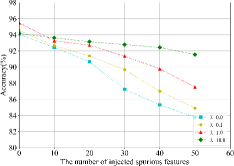
Figure 3: Ablation experiments on the value of parameter $\lambda$.

Based on Figure 3, we can draw the following conclusions: when no additional spurious features are added, the model’s performance improves as $\lambda$ increases within a certain range ($\lambda<1.0$). Besides, for sufficiently large values of $\lambda$ (e.g., $\lambda\geq 1.0$), larger values of $\lambda$ (such as $\lambda=10.0$) help force the model to learn knowledge from features that are completely unaffected by the environment, as represented by $X_{1}$ in Figure 1(c). This comes at the cost of sacrificing a certain level of accuracy since some features that are causally related to the prediction $Y$, such as $X_{2}$, are ignored, which to some extent violates the sufficiency condition (Condition 3). However, the model exhibits inclusiveness towards additionally added confusable spurious features. On the other hand, smaller values of $\lambda$ (e.g., $\lambda=1.0$) allow the model to learn knowledge from $X_{2}$, resulting in better initial performance. However, as the number of confusable spurious features similar to $X_{2}$ (such as $X_{4}$) increases, the OOD (out-of-distribution) performance deteriorates at a relatively faster rate due to the difficulty of distinguishing between $X_{2}$ and $X_{4}$.

D.6.3 Influence of $\beta$

We analyzed the impact of hyperparameter $\beta$ on performance, as shown in Table 9. The experiments were conducted on the synthetic dataset Cora. Here, we report the average accuracy for each test. Additionally, to validate the analysis in Section B.2, we randomly perturbed 5% of the edges in the test graphs based on DICE [47] and evaluated the model’s sensitivity to structural changes.

Table 9: The ablation study reults on different value of parameter $\beta$.

IENE-re	$\beta=0$	$\beta=0.01$	$\beta=0.1$	$\beta=1.0$	$\beta=5.0$	$\beta=10.0$
Original test data	93.99	94.62	95.26	95.58	95.17	94.21
+Random noise	91.73	92.51	93.28	93.93	93.67	92.78
Decrease	2.26	2.11	1.98	1.65	1.50	1.43

The results indicate that choosing the appropriate value for parameter $\beta$ is a determining factor for the model’s performance. As $\beta$ increases within a certain range, the OOD (out-of-distribution) performance improves. Additionally, larger values of $\beta$ tend to enable the model to learn invariant features that can adapt to variations of structural environment.

D.7 More Comparisons

Due to space limitations in the main text, we will present a comparison of some methods here. As shown in Table 10, our method still maintains superior performance.

Table 10: Comparison between IENE and other methods using GCN as Backbone.

Method	Cora	Amaz-Photo	Twitch-E	FB-100	Elliptic	OGB-Arxiv
SRGNN	92.43$\pm$ 2.48	93.85$\pm$1.31	56.04$\pm$1.63	52.91$\pm$1.60	64.76$\pm$3.59	44.24$\pm$1.78
LISA	93.85 $\pm$1.91	94.22 $\pm$1.06	57.83$\pm$2.16	53.17$\pm$1.39	64.39$\pm$2.62	43.49$\pm$0.71
IENE	95.58 $\pm$2.07	96.40 $\pm$1.80	61.87 $\pm$1.43	53.73 $\pm$2.65	67.90 $\pm$3.31	44.85 $\pm$0.31

D.8 Performance on In-distribution Data and Different Subsets

To verify the stability of our model on different data, we have supplemented the experimental results with in-distribution data on six datasets and various test subsets on Twitch and Arxiv, as shown in Table 11 to 13.

Table 11: The performance of IENE on In-distribution dataset.

	Cora	Amaz-Photo	Twitch-E	FB-100	Elliptic	OGB-Arxiv
ERM	94.80$\pm$ 0.25	95.49$\pm$0.21	71.41$\pm$0.03	59.31$\pm$0.32	74.87$\pm$0.12	47.21$\pm$0.45
IENE	97.33 $\pm$0.27	96.71 $\pm$0.38	71.27$\pm$0.08	59.52$\pm$0.40	75.18$\pm$0.48	48.73$\pm$0.30

Table 12: The performance of IENE on different subgraphs of Twitch.

	ES	FR	PTBR	RU	TW
ERM	60.73$\pm$ 2.75	56.41$\pm$2.14	59.39$\pm$1.80	45.77$\pm$1.55	47.90$\pm$1.76
IENE	63.74 $\pm$1.43	61.25 $\pm$1.05	64.85$\pm$1.11	56.26$\pm$0.52	57.59$\pm$0.83

Table 13: The performance of IENE on different publication years of Arxiv.

	2014-2016	2016-2018	2018-2020
ERM	42.83$\pm$ 0.93	41.58$\pm$1.67	40.36$\pm$0.79
IENE	46.39 $\pm$0.44	44.70 $\pm$0.92	43.46$\pm$0.53

Appendix E Hyperparameter Settings and Experimental Details

Table 14: Hyperparameter settings for the experiments.

Dataset	$Learning\ rate$	$K$	$\lambda$	$\beta$	$\eta$	$Learning\ ratefor\ u,d,w$	$num\_sample$
Cora	[0.005,0.01]	[2,3,4]	4.0	1.0	1.0	[0.005,0.01,0.05]	[1,3,5,7]
Amz-Photo	[0.01,0.05]	[3,4]	4.0	1.0	1.0	[0.001,0.1,0.5]	[1,3,5,7]
Twitch-E	[0.01,0.05]	[2,3,4]	4.0	3.0	1.0	[0.05,0.1]	[1,3,5,7]
FB-100	[0.005,0.01]	[2,3,4]	4.0	1.0	1.0	[0.05,0.1]	[1,3,5,7]
Elliptic	[0.005,0.01]	[2,3,4]	1.0	0.5	1.0	[0.01,0.05,0.1]	[1,3,5,7]
OGB-Arxiv	[0.001,0.01]	[2,3,4]	1.0	1.0	1.0	[0.05,0.1]	[1,3,5,7]

In this section, we will present the experimental details of Section 4. All experiments were conducted on an Nvidia A40 (48G) GPU, and the hyperparameters used for the methods proposed in Section 4 are shown in Table 14. The encoders and decoders used in all experiments are GNNs, and the classifier is a 2-layer MLP with 32 neurons. Here, we use the ReLU activation function [28] in all the networks. The output layers of the encoders $u(\cdot)$ and $\Phi(\cdot)$ are activated using the tanh function [52]. Hyperparameters in different network may be different, and we fine-tune these hyperparameters through a grid search method across 10 trials.

We primarily utilize the Adam optimizer for parameter updates [19], except for $u(\cdot)$, $\Phi(\cdot)$, $d(\cdot)$ and $w(\cdot)$ which use the SGD optimizer [5] to enhance the robustness of adversarial training.

The complete and reproducible code for our work has been anonymously submitted to: https://anonymous.4open.science/r/IENE-code

Appendix F Related Work

F.1 Invariant Learning

Invariant learning is a technique aimed at discovering invariant features to achieve out of distribution (OOD) generalization. Invariant features, denoted as $X_{i}$, exhibit stable correlations with the target Y when distribution shifts, while spurious features $X_{s}$ are unstable. In general, models relying on invariant features maintain robust on OOD data due to stable correlations when violating the independent and identically distributed (IID) assumption. Conversely, spurious features $X_{s}$ can lead to significant performance degradation [2]. [34], starting from causal theory, first investigated the fact that invariance can infer causal structures under necessary conditions, proposing Invariant Causal Prediction (ICP). Invariant Risk Minimization (IRM) is introduced to learn the optimal invariant associations across different environment partitions provided in the training data [2]. To further explore the capabilities of IRM, some literature combines multi-objective optimization with game theory [1, 9] or conducts invariant representation learning through adversarial training [6, 54]. REx [22] encourages reducing training risk while increasing similarity in training risk under the variance risk extrapolation paradigm. GroupDRO [38] has a similar problem setting to IRM, which obtains a robust model by reducing the worst-case training loss on a predefined set of groups.

However, most existing methods, including the aforementioned ones, greatly rely on additional environment labels explicitly provided in the training dataset. Such annotations for nodes on graph data are often unavailable and costly to collect, making these invariant learning methods impractical for real-world data [12, 30]. It has led to multiple efforts in performing invariant learning without the need for explicitly provided environment partitions. [41] utilize clustering techniques to partition the training data into different groups, then incorporate the labels of these groups as noise supervision into a distributionally robust optimization objective. EIIL [12] addresses the issue through a two-stage training involving biased model environment reasoning and sequence invariance learning for environment reasoning. Heterogeneous Risk Minimization (HRM) [30] jointly learns latent heterogeneity and invariance by using an identification module and an invariance predictor, respectively. ZIN [29] demonstrates that additional auxiliary variables provided by metadata of the dataset can be used for environment inference and subsequent invariant learning. TIVA [43] attempts to automatically learn environment partitions using target-independent variable $X_{z}$ ($X_{z}\bot Y$). However, on one hand, the performance of environment partitioning is limited due to the insufficient discovery of diverse environment factors; on the other hand, the assumption that $X_{z}$ can be used to partition the environment remains challenging to verify because $X_{z}$ may not have explicit physical meanings in many datasets.

In this work, we learn both environmental representations and invariant representations in a disentangled information bottleneck framework. We use environmental representation as auxiliary information for environmental reasoning and invariant representation as input for downstream tasks. Compared to the aforementioned methods, our approach is conducive to extracting more environmental information and promoting mutual learning between environmental learning and invariant learning.

F.2 Invariant Learning on Graph

Invariant learning on graphs can be more complex due to the various forms of distribution shifts, such as in features and structures, making it challenging to identify invariance. Recently, there has been widespread interest in exploring the out-of-distribution (OOD) generalization capability of GNNs. In particular, [4] focused on learning size-invariant representations to address distribution shifts related to graph size. DIR [51] created multiple randomly paired intervention graphs to achieve the goal of invariant causal representation learning across different distributions, enhancing generalization. GIL [25], through joint optimization of three custom modules, captured the invariant relationships between the structural information and labels of predicted graphs in mixed latent environments. CIGA [8] used causal models to characterize changes in distribution. MoleOOD [55] improved the robustness of molecular learning and could infer the environment in a data-driven manner. LISA [59] proposes a model-agnostic label-invariant subgraph augmentation framework to generate augmented environments with consistent predictive relationships for graph OOD generalization. These efforts have primarily centered on graph-level tasks, emphasizing the extraction of core subgraphs while generally overlooking the more challenging node-level tasks with multiple latent environments. In contrast, our work addresses the OOD problem in node-level tasks on graphs.

Some works addressing semi-supervised node classification in non-I.I.D. settings have been proposed to focus on the adaptability of GNNs under distribution shifts. For instance, SR-GNN [62] is designed to interpret the distribution differences between biased training data and the true inference distribution of the graph. CATs [16] introduced a joint attention mechanism considering structural perturbations to enhance the model’s generalization to structural biases. BA-GNN [10] improved the model’s generalization by identifying biases and learning invariant features. DGNN [14] introduced the idea of variable decorrelation in GNNs to mitigate the impact of label selection bias. However, designing models specifically for certain types of biases may not truly enhance generalization ability in real-world applications due to the presence of confounding biases. EERM [49], learns invariant representations of nodes by training multiple context generators to maximize the risk differences from multiple virtual environments. FLOOD [31] proposes an invariant learning component to construct multiple environments from graph data augmentation and learns invariant representations under risk extrapolation. However, EERM and FLOOD cannot guarantee the quality of the generated views during data augmentation, making it difficult to provide reliable support for invariant learning. Because view generators may take shortcuts to achieve their objectives, such as increasing risk differences in different environments by adding varying degrees of noise or reducing the amount of information, violating the assumption of environmental heterogeneity. CIE [7] introduces the independence constraint to improve discriminability and stability of causal and spurious features in complex biased environments and mitigates spurious correlations by implementing the backdoor adjustment. CaNet [48] uses a new learning objective derived from causal inference that coordinates an environment estimator and a mixture-of-expert GNN predictor to counteract the confounding bias in training data. These two works combine the idea of causal reasoning, aiming to eliminate confounding bias in the data.

Appendix G Limitations

The limitations of IENE have been partially discussed in sections 3.3.2 and B.5 that we discussed the scenarios where IENE can successfully identify invariant features. Here, we will discuss some other limitations.

Dependence on assumptions. The success of IENE still relies on some common assumptions that are required in many invariant learning works. Therefore, in some specific cases, it may not be able to recognize all invariant features.

Requirements for computing resource. Although the environmental extrapolation module can potentially enhance generalization performance by identifying more invariant features, it significantly increases the model’s time and memory overhead on some datasets, as shown in Table 3. This may not be user-friendly for resource-constrained scenarios.

Scalability. The scalability of the model on large-scale and complex graphs remains to be further validated. We believe that IENE possesses scalability since it is a relatively flexible learning framework where the backbone network can be freely switched and potentially integrated with other frameworks. Moreover, our empirical results indicate that switching the backbone network does not affect the effectiveness of the framework. Therefore, it is possible to extend IENE to large-scale graphs by employing local graph sampling strategies or sampling-based networks such as GraphSAGE as the backbone. Similarly, adopting heterogeneous graph convolutional networks as the backbone can enable extension to heterogeneous graphs. While this idea seems simple, it may be feasible, and we plan to further validate the capabilities of IENE on large-scale and heterogeneous graph datasets in the future.

NeurIPS Paper Checklist

1. Claims

2. Question: Do the main claims made in the abstract and introduction accurately reflect the paper’s contributions and scope?

3. Answer: [Yes]

4. Justification: We confirm that the main claims presented in the abstract and introduction reflect the contribution and scope of the paper.

5. Guidelines:

   • The answer NA means that the abstract and introduction do not include the claims made in the paper.

   • The abstract and/or introduction should clearly state the claims made, including the contributions made in the paper and important assumptions and limitations. A No or NA answer to this question will not be perceived well by the reviewers.

   • The claims made should match theoretical and experimental results, and reflect how much the results can be expected to generalize to other settings.

   • It is fine to include aspirational goals as motivation as long as it is clear that these goals are not attained by the paper.

6. Limitations

7. Question: Does the paper discuss the limitations of the work performed by the authors?

8. Answer: [Yes]

9. Justification: We discussed the limitations of our work in the appendix G.

10. Guidelines:

    • The answer NA means that the paper has no limitation while the answer No means that the paper has limitations, but those are not discussed in the paper.

    • The authors are encouraged to create a separate "Limitations" section in their paper.

    • The paper should point out any strong assumptions and how robust the results are to violations of these assumptions (e.g., independence assumptions, noiseless settings, model well-specification, asymptotic approximations only holding locally). The authors should reflect on how these assumptions might be violated in practice and what the implications would be.

    • The authors should reflect on the scope of the claims made, e.g., if the approach was only tested on a few datasets or with a few runs. In general, empirical results often depend on implicit assumptions, which should be articulated.

    • The authors should reflect on the factors that influence the performance of the approach. For example, a facial recognition algorithm may perform poorly when image resolution is low or images are taken in low lighting. Or a speech-to-text system might not be used reliably to provide closed captions for online lectures because it fails to handle technical jargon.

    • The authors should discuss the computational efficiency of the proposed algorithms and how they scale with dataset size.

    • If applicable, the authors should discuss possible limitations of their approach to address problems of privacy and fairness.

    • While the authors might fear that complete honesty about limitations might be used by reviewers as grounds for rejection, a worse outcome might be that reviewers discover limitations that aren’t acknowledged in the paper. The authors should use their best judgment and recognize that individual actions in favor of transparency play an important role in developing norms that preserve the integrity of the community. Reviewers will be specifically instructed to not penalize honesty concerning limitations.

11. Theory Assumptions and Proofs

12. Question: For each theoretical result, does the paper provide the full set of assumptions and a complete (and correct) proof?

13. Answer: [Yes]

14. Justification: We have listed the used assumptions in Appendix B.6 and provided proof in Appendix C.

15. Guidelines:

    • The answer NA means that the paper does not include theoretical results.

    • All the theorems, formulas, and proofs in the paper should be numbered and cross-referenced.

    • All assumptions should be clearly stated or referenced in the statement of any theorems.

    • The proofs can either appear in the main paper or the supplemental material, but if they appear in the supplemental material, the authors are encouraged to provide a short proof sketch to provide intuition.

    • Inversely, any informal proof provided in the core of the paper should be complemented by formal proofs provided in appendix or supplemental material.

    • Theorems and Lemmas that the proof relies upon should be properly referenced.

16. Experimental Result Reproducibility

17. Question: Does the paper fully disclose all the information needed to reproduce the main experimental results of the paper to the extent that it affects the main claims and/or conclusions of the paper (regardless of whether the code and data are provided or not)?

18. Answer: [Yes]

19. Justification: We provide detailed model parameter information in Appendix E and attach reproducible code. And the dataset used in the experiment is shown in the code description.

20. Guidelines:

    • The answer NA means that the paper does not include experiments.

    • If the paper includes experiments, a No answer to this question will not be perceived well by the reviewers: Making the paper reproducible is important, regardless of whether the code and data are provided or not.

    • If the contribution is a dataset and/or model, the authors should describe the steps taken to make their results reproducible or verifiable.

    • Depending on the contribution, reproducibility can be accomplished in various ways. For example, if the contribution is a novel architecture, describing the architecture fully might suffice, or if the contribution is a specific model and empirical evaluation, it may be necessary to either make it possible for others to replicate the model with the same dataset, or provide access to the model. In general. releasing code and data is often one good way to accomplish this, but reproducibility can also be provided via detailed instructions for how to replicate the results, access to a hosted model (e.g., in the case of a large language model), releasing of a model checkpoint, or other means that are appropriate to the research performed.

    • While NeurIPS does not require releasing code, the conference does require all submissions to provide some reasonable avenue for reproducibility, which may depend on the nature of the contribution. For example

      1. If the contribution is primarily a new algorithm, the paper should make it clear how to reproduce that algorithm.

      2. If the contribution is primarily a new model architecture, the paper should describe the architecture clearly and fully.

      3. If the contribution is a new model (e.g., a large language model), then there should either be a way to access this model for reproducing the results or a way to reproduce the model (e.g., with an open-source dataset or instructions for how to construct the dataset).

      4. We recognize that reproducibility may be tricky in some cases, in which case authors are welcome to describe the particular way they provide for reproducibility. In the case of closed-source models, it may be that access to the model is limited in some way (e.g., to registered users), but it should be possible for other researchers to have some path to reproducing or verifying the results.

21. Open access to data and code

22. Question: Does the paper provide open access to the data and code, with sufficient instructions to faithfully reproduce the main experimental results, as described in supplemental material?

23. Answer: [Yes]

24. Justification: We provide detailed model parameter information in Appendix E and attach reproducible code. And the dataset used in the experiment is shown in the code description.

25. Guidelines:

    • The answer NA means that paper does not include experiments requiring code.

    • Please see the NeurIPS code and data submission guidelines (https://nips.cc/public/guides/CodeSubmissionPolicy) for more details.

    • While we encourage the release of code and data, we understand that this might not be possible, so “No” is an acceptable answer. Papers cannot be rejected simply for not including code, unless this is central to the contribution (e.g., for a new open-source benchmark).

    • The instructions should contain the exact command and environment needed to run to reproduce the results. See the NeurIPS code and data submission guidelines (https://nips.cc/public/guides/CodeSubmissionPolicy) for more details.

    • The authors should provide instructions on data access and preparation, including how to access the raw data, preprocessed data, intermediate data, and generated data, etc.

    • The authors should provide scripts to reproduce all experimental results for the new proposed method and baselines. If only a subset of experiments are reproducible, they should state which ones are omitted from the script and why.

    • At submission time, to preserve anonymity, the authors should release anonymized versions (if applicable).

    • Providing as much information as possible in supplemental material (appended to the paper) is recommended, but including URLs to data and code is permitted.

26. Experimental Setting/Details

27. Question: Does the paper specify all the training and test details (e.g., data splits, hyperparameters, how they were chosen, type of optimizer, etc.) necessary to understand the results?

28. Answer: [Yes]

29. Justification: We provide detailed model parameter information in Appendix E and attach reproducible code. And the dataset used in the experiment is shown in the code description.

30. Guidelines:

    • The answer NA means that the paper does not include experiments.

    • The experimental setting should be presented in the core of the paper to a level of detail that is necessary to appreciate the results and make sense of them.

    • The full details can be provided either with the code, in appendix, or as supplemental material.

31. Experiment Statistical Significance

32. Question: Does the paper report error bars suitably and correctly defined or other appropriate information about the statistical significance of the experiments?

33. Answer: [Yes]

34. Justification: As we demonstrated in Section 4, we repeated the experiment ten times and reported the mean value and standard deviation of the results. In addition, instructions were provided on how to reproduce the results.

35. Guidelines:

    • The answer NA means that the paper does not include experiments.

    • The authors should answer "Yes" if the results are accompanied by error bars, confidence intervals, or statistical significance tests, at least for the experiments that support the main claims of the paper.

    • The factors of variability that the error bars are capturing should be clearly stated (for example, train/test split, initialization, random drawing of some parameter, or overall run with given experimental conditions).

    • The method for calculating the error bars should be explained (closed form formula, call to a library function, bootstrap, etc.)

    • The assumptions made should be given (e.g., Normally distributed errors).

    • It should be clear whether the error bar is the standard deviation or the standard error of the mean.

    • It is OK to report 1-sigma error bars, but one should state it. The authors should preferably report a 2-sigma error bar than state that they have a 96% CI, if the hypothesis of Normality of errors is not verified.

    • For asymmetric distributions, the authors should be careful not to show in tables or figures symmetric error bars that would yield results that are out of range (e.g. negative error rates).

    • If error bars are reported in tables or plots, The authors should explain in the text how they were calculated and reference the corresponding figures or tables in the text.

36. Experiments Compute Resources

37. Question: For each experiment, does the paper provide sufficient information on the computer resources (type of compute workers, memory, time of execution) needed to reproduce the experiments?

38. Answer: [Yes]

39. Justification: We introduced the comparison of computational efficiency in Section 4.2(c), and the results are shown in Table 3.

40. Guidelines:

    • The answer NA means that the paper does not include experiments.

    • The paper should indicate the type of compute workers CPU or GPU, internal cluster, or cloud provider, including relevant memory and storage.

    • The paper should provide the amount of compute required for each of the individual experimental runs as well as estimate the total compute.

    • The paper should disclose whether the full research project required more compute than the experiments reported in the paper (e.g., preliminary or failed experiments that didn’t make it into the paper).

41. Code Of Ethics

42. Question: Does the research conducted in the paper conform, in every respect, with the NeurIPS Code of Ethics https://neurips.cc/public/EthicsGuidelines?

43. Answer: [Yes]

44. Justification: Yes, our research complies with NeurIPS ethical standards.

45. Guidelines:

    • The answer NA means that the authors have not reviewed the NeurIPS Code of Ethics.

    • If the authors answer No, they should explain the special circumstances that require a deviation from the Code of Ethics.

    • The authors should make sure to preserve anonymity (e.g., if there is a special consideration due to laws or regulations in their jurisdiction).

46. Broader Impacts

47. Question: Does the paper discuss both potential positive societal impacts and negative societal impacts of the work performed?

48. Answer: [N/A]

49. Justification: Our work belongs to basic research and has no significant social impact.

50. Guidelines:

    • The answer NA means that there is no societal impact of the work performed.

    • If the authors answer NA or No, they should explain why their work has no societal impact or why the paper does not address societal impact.

    • Examples of negative societal impacts include potential malicious or unintended uses (e.g., disinformation, generating fake profiles, surveillance), fairness considerations (e.g., deployment of technologies that could make decisions that unfairly impact specific groups), privacy considerations, and security considerations.

    • The conference expects that many papers will be foundational research and not tied to particular applications, let alone deployments. However, if there is a direct path to any negative applications, the authors should point it out. For example, it is legitimate to point out that an improvement in the quality of generative models could be used to generate deepfakes for disinformation. On the other hand, it is not needed to point out that a generic algorithm for optimizing neural networks could enable people to train models that generate Deepfakes faster.

    • The authors should consider possible harms that could arise when the technology is being used as intended and functioning correctly, harms that could arise when the technology is being used as intended but gives incorrect results, and harms following from (intentional or unintentional) misuse of the technology.

    • If there are negative societal impacts, the authors could also discuss possible mitigation strategies (e.g., gated release of models, providing defenses in addition to attacks, mechanisms for monitoring misuse, mechanisms to monitor how a system learns from feedback over time, improving the efficiency and accessibility of ML).

51. Safeguards

52. Question: Does the paper describe safeguards that have been put in place for responsible release of data or models that have a high risk for misuse (e.g., pretrained language models, image generators, or scraped datasets)?

53. Answer: [N/A]

54. Justification: the paper poses no such risks.

55. Guidelines:

    • The answer NA means that the paper poses no such risks.

    • Released models that have a high risk for misuse or dual-use should be released with necessary safeguards to allow for controlled use of the model, for example by requiring that users adhere to usage guidelines or restrictions to access the model or implementing safety filters.

    • Datasets that have been scraped from the Internet could pose safety risks. The authors should describe how they avoided releasing unsafe images.

    • We recognize that providing effective safeguards is challenging, and many papers do not require this, but we encourage authors to take this into account and make a best faith effort.

56. Licenses for existing assets

57. Question: Are the creators or original owners of assets (e.g., code, data, models), used in the paper, properly credited and are the license and terms of use explicitly mentioned and properly respected?

58. Answer: [Yes]

59. Justification: All assets used in this paper have clear references and are publicly available.

60. Guidelines:

    • The answer NA means that the paper does not use existing assets.

    • The authors should cite the original paper that produced the code package or dataset.

    • The authors should state which version of the asset is used and, if possible, include a URL.

    • The name of the license (e.g., CC-BY 4.0) should be included for each asset.

    • For scraped data from a particular source (e.g., website), the copyright and terms of service of that source should be provided.

    • If assets are released, the license, copyright information, and terms of use in the package should be provided. For popular datasets, paperswithcode.com/datasets has curated licenses for some datasets. Their licensing guide can help determine the license of a dataset.

    • For existing datasets that are re-packaged, both the original license and the license of the derived asset (if it has changed) should be provided.

    • If this information is not available online, the authors are encouraged to reach out to the asset’s creators.

61. New Assets

62. Question: Are new assets introduced in the paper well documented and is the documentation provided alongside the assets?

63. Answer: [Yes]

64. Justification: The code we release and the dataset we use are well documented in the code repository documentation.

65. Guidelines:

    • The answer NA means that the paper does not release new assets.

    • Researchers should communicate the details of the dataset/code/model as part of their submissions via structured templates. This includes details about training, license, limitations, etc.

    • The paper should discuss whether and how consent was obtained from people whose asset is used.

    • At submission time, remember to anonymize your assets (if applicable). You can either create an anonymized URL or include an anonymized zip file.

66. Crowdsourcing and Research with Human Subjects

67. Question: For crowdsourcing experiments and research with human subjects, does the paper include the full text of instructions given to participants and screenshots, if applicable, as well as details about compensation (if any)?

68. Answer: [N/A]

69. Justification: the paper does not involve crowdsourcing nor research with human subjects.

70. Guidelines:

    • The answer NA means that the paper does not involve crowdsourcing nor research with human subjects.

    • Including this information in the supplemental material is fine, but if the main contribution of the paper involves human subjects, then as much detail as possible should be included in the main paper.

    • According to the NeurIPS Code of Ethics, workers involved in data collection, curation, or other labor should be paid at least the minimum wage in the country of the data collector.

71. Institutional Review Board (IRB) Approvals or Equivalent for Research with Human Subjects

72. Question: Does the paper describe potential risks incurred by study participants, whether such risks were disclosed to the subjects, and whether Institutional Review Board (IRB) approvals (or an equivalent approval/review based on the requirements of your country or institution) were obtained?

73. Answer: [N/A]

74. Justification: the paper does not involve crowdsourcing nor research with human subjects.

75. Guidelines:

    • The answer NA means that the paper does not involve crowdsourcing nor research with human subjects.

    • Depending on the country in which research is conducted, IRB approval (or equivalent) may be required for any human subjects research. If you obtained IRB approval, you should clearly state this in the paper.

    • We recognize that the procedures for this may vary significantly between institutions and locations, and we expect authors to adhere to the NeurIPS Code of Ethics and the guidelines for their institution.

    • For initial submissions, do not include any information that would break anonymity (if applicable), such as the institution conducting the review.

References

- [1] Kartik Ahuja, Karthikeyan Shanmugam, Kush R. Varshney and Amit Dhurandhar “Invariant Risk Minimization Games” In Proceedings of the 37th International Conference on Machine Learning, ICML 2020, 13-18 July 2020, Virtual Event 119, Proceedings of Machine Learning Research PMLR, 2020, pp. 145–155
- [2] Martín Arjovsky, Léon Bottou, Ishaan Gulrajani and David Lopez-Paz “Invariant Risk Minimization” In CoRR abs/1907.02893, 2019 arXiv:1907.02893
- [3] Yoshua Bengio et al. “A Meta-Transfer Objective for Learning to Disentangle Causal Mechanisms” In 8th International Conference on Learning Representations, ICLR 2020, Addis Ababa, Ethiopia, April 26-30, 2020 OpenReview.net, 2020
- [4] Beatrice Bevilacqua, Yangze Zhou and Bruno Ribeiro “Size-Invariant Graph Representations for Graph Classification Extrapolations” In Proceedings of the 38th International Conference on Machine Learning, ICML 2021, 18-24 July 2021, Virtual Event 139, Proceedings of Machine Learning Research PMLR, 2021, pp. 837–851
- [5] Léon Bottou “Stochastic Gradient Descent Tricks” In Neural Networks: Tricks of the Trade - Second Edition 7700, Lecture Notes in Computer Science Springer, 2012, pp. 421–436 DOI: 10.1007/978-3-642-35289-8\_25
- [6] Shiyu Chang, Yang Zhang, Mo Yu and Tommi S. Jaakkola “Invariant Rationalization” In Proceedings of the 37th International Conference on Machine Learning, ICML 2020, 13-18 July 2020, Virtual Event 119, Proceedings of Machine Learning Research PMLR, 2020, pp. 1448–1458
- [7] Guoxin Chen et al. “Causality and Independence Enhancement for Biased Node Classification” In Proceedings of the 32nd ACM International Conference on Information and Knowledge Management, CIKM 2023, Birmingham, United Kingdom, October 21-25, 2023 ACM, 2023, pp. 203–212 DOI: 10.1145/3583780.3614804
- [8] Yongqiang Chen et al. “Learning Causally Invariant Representations for Out-of-Distribution Generalization on Graphs” In Advances in Neural Information Processing Systems 35: Annual Conference on Neural Information Processing Systems 2022, NeurIPS 2022, New Orleans, LA, USA, November 28 - December 9, 2022, 2022
- [9] Yongqiang Chen et al. “Pareto Invariant Risk Minimization: Towards Mitigating the Optimization Dilemma in Out-of-Distribution Generalization” In The Eleventh International Conference on Learning Representations, ICLR 2023, Kigali, Rwanda, May 1-5, 2023 OpenReview.net, 2023
- [10] Zhengyu Chen, Teng Xiao and Kun Kuang “BA-GNN: On Learning Bias-Aware Graph Neural Network” In 38th IEEE International Conference on Data Engineering, ICDE 2022, Kuala Lumpur, Malaysia, May 9-12, 2022 IEEE, 2022, pp. 3012–3024 DOI: 10.1109/ICDE53745.2022.00271
- [11] Eli Chien, Jianhao Peng, Pan Li and Olgica Milenkovic “Adaptive Universal Generalized PageRank Graph Neural Network” In 9th International Conference on Learning Representations, ICLR 2021, Virtual Event, Austria, May 3-7, 2021 OpenReview.net, 2021
- [12] Elliot Creager, Jörn-Henrik Jacobsen and Richard S. Zemel “Environment Inference for Invariant Learning” In Proceedings of the 38th International Conference on Machine Learning, ICML 2021, 18-24 July 2021, Virtual Event 139, Proceedings of Machine Learning Research PMLR, 2021, pp. 2189–2200
- [13] Logan Engstrom et al. “Exploring the Landscape of Spatial Robustness” In Proceedings of the 36th International Conference on Machine Learning, ICML 2019, 9-15 June 2019, Long Beach, California, USA 97, Proceedings of Machine Learning Research PMLR, 2019, pp. 1802–1811
- [14] Shaohua Fan et al. “Debiased Graph Neural Networks with Agnostic Label Selection Bias” In CoRR abs/2201.07708, 2022 arXiv:2201.07708
- [15] William L. Hamilton, Zhitao Ying and Jure Leskovec “Inductive Representation Learning on Large Graphs” In Advances in Neural Information Processing Systems 30: Annual Conference on Neural Information Processing Systems 2017, December 4-9, 2017, Long Beach, CA, USA, 2017, pp. 1024–1034
- [16] Tiantian He, Yew Soon Ong and Lu Bai “Learning Conjoint Attentions for Graph Neural Nets” In Advances in Neural Information Processing Systems 34: Annual Conference on Neural Information Processing Systems 2021, NeurIPS 2021, December 6-14, 2021, virtual, 2021, pp. 2641–2653
- [17] Weihua Hu et al. “Open Graph Benchmark: Datasets for Machine Learning on Graphs” In Advances in Neural Information Processing Systems 33: Annual Conference on Neural Information Processing Systems 2020, NeurIPS 2020, December 6-12, 2020, virtual, 2020
- [18] Wei Jin et al. “Empowering Graph Representation Learning with Test-Time Graph Transformation” In The Eleventh International Conference on Learning Representations, ICLR 2023, Kigali, Rwanda, May 1-5, 2023 OpenReview.net, 2023
- [19] Diederik P. Kingma and Jimmy Ba “Adam: A Method for Stochastic Optimization” In 3rd International Conference on Learning Representations, ICLR 2015, San Diego, CA, USA, May 7-9, 2015, Conference Track Proceedings, 2015
- [20] Thomas N. Kipf and Max Welling “Semi-Supervised Classification with Graph Convolutional Networks” In 5th International Conference on Learning Representations, ICLR 2017, Toulon, France, April 24-26, 2017, Conference Track Proceedings OpenReview.net, 2017
- [21] Simon Kornblith, Mohammad Norouzi, Honglak Lee and Geoffrey E. Hinton “Similarity of Neural Network Representations Revisited” In Proceedings of the 36th International Conference on Machine Learning, ICML 2019, 9-15 June 2019, Long Beach, California, USA 97, Proceedings of Machine Learning Research PMLR, 2019, pp. 3519–3529
- [22] David Krueger et al. “Out-of-Distribution Generalization via Risk Extrapolation (REx)” In Proceedings of the 38th International Conference on Machine Learning, ICML 2021, 18-24 July 2021, Virtual Event 139, Proceedings of Machine Learning Research PMLR, 2021, pp. 5815–5826
- [23] Kun Kuang et al. “Stable Prediction with Model Misspecification and Agnostic Distribution Shift” In The Thirty-Fourth AAAI Conference on Artificial Intelligence, AAAI 2020, The Thirty-Second Innovative Applications of Artificial Intelligence Conference, IAAI 2020, The Tenth AAAI Symposium on Educational Advances in Artificial Intelligence, EAAI 2020, New York, NY, USA, February 7-12, 2020 AAAI Press, 2020, pp. 4485–4492 DOI: 10.1609/AAAI.V34I04.5876
- [24] Julius Kügelgen et al. “Self-Supervised Learning with Data Augmentations Provably Isolates Content from Style” In Advances in Neural Information Processing Systems 34: Annual Conference on Neural Information Processing Systems 2021, NeurIPS 2021, December 6-14, 2021, virtual, 2021, pp. 16451–16467
- [25] Haoyang Li, Ziwei Zhang, Xin Wang and Wenwu Zhu “Learning Invariant Graph Representations for Out-of-Distribution Generalization” In Advances in Neural Information Processing Systems 35: Annual Conference on Neural Information Processing Systems 2022, NeurIPS 2022, New Orleans, LA, USA, November 28 - December 9, 2022, 2022
- [26] Haoyang Li, Xin Wang, Ziwei Zhang and Wenwu Zhu “Out-Of-Distribution Generalization on Graphs: A Survey” In CoRR abs/2202.07987, 2022 arXiv:2202.07987
- [27] Pengbo Li, Hang Yu, Xiangfeng Luo and Jia Wu “LGM-GNN: A Local and Global Aware Memory-Based Graph Neural Network for Fraud Detection” In IEEE Trans. Big Data 9.4, 2023, pp. 1116–1127 DOI: 10.1109/TBDATA.2023.3234529
- [28] Yuanzhi Li and Yang Yuan “Convergence Analysis of Two-layer Neural Networks with ReLU Activation” In Advances in Neural Information Processing Systems 30: Annual Conference on Neural Information Processing Systems 2017, December 4-9, 2017, Long Beach, CA, USA, 2017, pp. 597–607
- [29] Yong Lin, Shengyu Zhu, Lu Tan and Peng Cui “ZIN: When and How to Learn Invariance Without Environment Partition?” In Advances in Neural Information Processing Systems 35: Annual Conference on Neural Information Processing Systems 2022, NeurIPS 2022, New Orleans, LA, USA, November 28 - December 9, 2022, 2022
- [30] Jiashuo Liu et al. “Heterogeneous Risk Minimization” In Proceedings of the 38th International Conference on Machine Learning, ICML 2021, 18-24 July 2021, Virtual Event 139, Proceedings of Machine Learning Research PMLR, 2021, pp. 6804–6814
- [31] Yang Liu et al. “FLOOD: A Flexible Invariant Learning Framework for Out-of-Distribution Generalization on Graphs” In Proceedings of the 29th ACM SIGKDD Conference on Knowledge Discovery and Data Mining, KDD 2023, Long Beach, CA, USA, August 6-10, 2023 ACM, 2023, pp. 1548–1558 DOI: 10.1145/3580305.3599355
- [32] Ziqi Pan, Li Niu, Jianfu Zhang and Liqing Zhang “Disentangled Information Bottleneck” In Thirty-Fifth AAAI Conference on Artificial Intelligence, AAAI 2021, Thirty-Third Conference on Innovative Applications of Artificial Intelligence, IAAI 2021, The Eleventh Symposium on Educational Advances in Artificial Intelligence, EAAI 2021, Virtual Event, February 2-9, 2021 AAAI Press, 2021, pp. 9285–9293 DOI: 10.1609/AAAI.V35I10.17120
- [33] Aldo Pareja et al. “EvolveGCN: Evolving Graph Convolutional Networks for Dynamic Graphs” In The Thirty-Fourth AAAI Conference on Artificial Intelligence, AAAI 2020, The Thirty-Second Innovative Applications of Artificial Intelligence Conference, IAAI 2020, The Tenth AAAI Symposium on Educational Advances in Artificial Intelligence, EAAI 2020, New York, NY, USA, February 7-12, 2020 AAAI Press, 2020, pp. 5363–5370 DOI: 10.1609/AAAI.V34I04.5984
- [34] Jonas Peters, Peter Bühlmann and Nicolai Meinshausen “Causal Inference by using Invariant Prediction: Identification and Confidence Intervals” In Journal of the Royal Statistical Society Series B: Statistical Methodology 78.5, 2016, pp. 947–1012 DOI: 10.1111/rssb.12167
- [35] Yu Rong, Wenbing Huang, Tingyang Xu and Junzhou Huang “DropEdge: Towards Deep Graph Convolutional Networks on Node Classification” In 8th International Conference on Learning Representations, ICLR 2020, Addis Ababa, Ethiopia, April 26-30, 2020 OpenReview.net, 2020
- [36] Elan Rosenfeld, Pradeep Kumar Ravikumar and Andrej Risteski “The Risks of Invariant Risk Minimization” In 9th International Conference on Learning Representations, ICLR 2021, Virtual Event, Austria, May 3-7, 2021 OpenReview.net, 2021
- [37] Benedek Rozemberczki, Carl Allen and Rik Sarkar “Multi-Scale attributed node embedding” In J. Complex Networks 9.2, 2021 DOI: 10.1093/COMNET/CNAB014
- [38] Shiori Sagawa, Pang Wei Koh, Tatsunori B. Hashimoto and Percy Liang “Distributionally Robust Neural Networks for Group Shifts: On the Importance of Regularization for Worst-Case Generalization” In CoRR abs/1911.08731, 2019 arXiv:1911.08731
- [39] Oleksandr Shchur, Maximilian Mumme, Aleksandar Bojchevski and Stephan Günnemann “Pitfalls of Graph Neural Network Evaluation” In CoRR abs/1811.05868, 2018 arXiv:1811.05868
- [40] Zheyan Shen, Peng Cui, Tong Zhang and Kun Kuang “Stable Learning via Sample Reweighting” In The Thirty-Fourth AAAI Conference on Artificial Intelligence, AAAI 2020, The Thirty-Second Innovative Applications of Artificial Intelligence Conference, IAAI 2020, The Tenth AAAI Symposium on Educational Advances in Artificial Intelligence, EAAI 2020, New York, NY, USA, February 7-12, 2020 AAAI Press, 2020, pp. 5692–5699 DOI: 10.1609/AAAI.V34I04.6024
- [41] Nimit Sharad Sohoni et al. “No Subclass Left Behind: Fine-Grained Robustness in Coarse-Grained Classification Problems” In Advances in Neural Information Processing Systems 33: Annual Conference on Neural Information Processing Systems 2020, NeurIPS 2020, December 6-12, 2020, virtual, 2020
- [42] Jiawei Su, Danilo Vasconcellos Vargas and Kouichi Sakurai “One Pixel Attack for Fooling Deep Neural Networks” In IEEE Trans. Evol. Comput. 23.5, 2019, pp. 828–841 DOI: 10.1109/TEVC.2019.2890858
- [43] Xiaoyu Tan et al. “Provably Invariant Learning without Domain Information” In International Conference on Machine Learning, ICML 2023, 23-29 July 2023, Honolulu, Hawaii, USA 202, Proceedings of Machine Learning Research PMLR, 2023, pp. 33563–33580
- [44] Amanda L. Traud, Peter J. Mucha and Mason A. Porter “Social Structure of Facebook Networks” In CoRR abs/1102.2166, 2011 arXiv:1102.2166
- [45] Petar Velickovic et al. “Graph Attention Networks” In 6th International Conference on Learning Representations, ICLR 2018, Vancouver, BC, Canada, April 30 - May 3, 2018, Conference Track Proceedings OpenReview.net, 2018
- [46] Wei Wang et al. “User-Context Collaboration and Tensor Factorization for GNN-Based Social Recommendation” In IEEE Trans. Netw. Sci. Eng. 10.6, 2023, pp. 3320–3330 DOI: 10.1109/TNSE.2023.3258427
- [47] Marcin Waniek, Tomasz P. Michalak, Talal Rahwan and Michael J. Wooldridge “Hiding Individuals and Communities in a Social Network” In CoRR abs/1608.00375, 2016 arXiv:1608.00375
- [48] Qitian Wu et al. “Graph Out-of-Distribution Generalization via Causal Intervention” In Proceedings of the ACM on Web Conference 2024, WWW 2024, Singapore, May 13-17, 2024 ACM, 2024, pp. 850–860 DOI: 10.1145/3589334.3645604
- [49] Qitian Wu, Hengrui Zhang, Junchi Yan and David Wipf “Handling Distribution Shifts on Graphs: An Invariance Perspective” In The Tenth International Conference on Learning Representations, ICLR 2022, Virtual Event, April 25-29, 2022 OpenReview.net, 2022
- [50] Xinglong Wu et al. “PDA-GNN: propagation-depth-aware graph neural networks for recommendation” In World Wide Web (WWW) 26.5, 2023, pp. 3585–3606 DOI: 10.1007/S11280-023-01200-Z
- [51] Yingxin Wu et al. “Discovering Invariant Rationales for Graph Neural Networks” In The Tenth International Conference on Learning Representations, ICLR 2022, Virtual Event, April 25-29, 2022 OpenReview.net, 2022
- [52] F. Xiao, Y. Honma and T. Kono “A simple algebraic interface capturing scheme using hyperbolic tangent function” In International Journal for Numerical Methods in Fluids 48.9, 2005, pp. 1023–1040 DOI: 10.1002/fld.975
- [53] Kaidi Xu et al. “Topology Attack and Defense for Graph Neural Networks: An Optimization Perspective” In Proceedings of the Twenty-Eighth International Joint Conference on Artificial Intelligence, IJCAI 2019, Macao, China, August 10-16, 2019 ijcai.org, 2019, pp. 3961–3967 DOI: 10.24963/IJCAI.2019/550
- [54] Yilun Xu and Tommi S. Jaakkola “Learning Representations that Support Robust Transfer of Predictors” In CoRR abs/2110.09940, 2021 arXiv:2110.09940
- [55] Nianzu Yang et al. “Learning Substructure Invariance for Out-of-Distribution Molecular Representations” In Advances in Neural Information Processing Systems 35: Annual Conference on Neural Information Processing Systems 2022, NeurIPS 2022, New Orleans, LA, USA, November 28 - December 9, 2022, 2022
- [56] Zhilin Yang, William W. Cohen and Ruslan Salakhutdinov “Revisiting Semi-Supervised Learning with Graph Embeddings” In Proceedings of the 33nd International Conference on Machine Learning, ICML 2016, New York City, NY, USA, June 19-24, 2016 48, JMLR Workshop and Conference Proceedings JMLR.org, 2016, pp. 40–48
- [57] Xiaoyan Yin et al. “AS-GNN: Rigging GNN-Based Social Status by Adversarial Attacks in Signed Social Networks” In IEEE Trans. Inf. Forensics Secur. 18, 2023, pp. 206–220 DOI: 10.1109/TIFS.2022.3219342
- [58] Yuning You et al. “Graph Contrastive Learning with Augmentations” In Advances in Neural Information Processing Systems 33: Annual Conference on Neural Information Processing Systems 2020, NeurIPS 2020, December 6-12, 2020, virtual, 2020
- [59] Junchi Yu, Jian Liang and Ran He “Mind the Label Shift of Augmentation-based Graph OOD Generalization” In 2023 IEEE/CVF Conference on Computer Vision and Pattern Recognition (CVPR), 2023, pp. 11620–11630 DOI: 10.1109/CVPR52729.2023.01118
- [60] Dan Zhang et al. “ApeGNN: Node-Wise Adaptive Aggregation in GNNs for Recommendation” In Proceedings of the ACM Web Conference 2023, WWW 2023, Austin, TX, USA, 30 April 2023 - 4 May 2023 ACM, 2023, pp. 759–769 DOI: 10.1145/3543507.3583530
- [61] Xiao Zhou, Yong Lin, Weizhong Zhang and Tong Zhang “Sparse Invariant Risk Minimization” In International Conference on Machine Learning, ICML 2022, 17-23 July 2022, Baltimore, Maryland, USA 162, Proceedings of Machine Learning Research PMLR, 2022, pp. 27222–27244
- [62] Qi Zhu, Natalia Ponomareva, Jiawei Han and Bryan Perozzi “Shift-Robust GNNs: Overcoming the Limitations of Localized Graph Training data” In Advances in Neural Information Processing Systems 34: Annual Conference on Neural Information Processing Systems 2021, NeurIPS 2021, December 6-14, 2021, virtual, 2021, pp. 27965–27977