Mechanisms of unstable blowup in a quadratic nonlinear Schrödinger equation

Abstract

In the work Cho et al. [Jpn. J. Ind. Appl. Math. 33 (2016): 145-166] the authors conjecture that the quadratic nonlinear Schrödinger equation (NLS) $iu_{t}=u_{xx}+u^{2}$ for $x\in\mathbb{T}$ is globally well-posed for real initial data. While this may be true in a generic sense, we present evidence that this conjecture is false. Moreover we conjecture that the set of real initial data which blows up under the NLS dynamics is the stable manifold of the zero equilibrium for the nonlinear heat equation $u_{t}=u_{xx}+u^{2}$.

1 Introduction

Determining whether solutions to a differential equation can blow up in finite time is important for understanding the scope of validity for a given model. The blowup of solutions can be easy to detect through direct numerical simulation if it occurs for a large open set of initial data, but detection may be difficult if the blowup set is unstable and has finite co-dimension. Indeed, unstable objects are by definition sensitive to perturbation, and numerically simulating a blowup solution to a PDE causes both the temporal and spatial resolution to diverge as the blowup time is approached. Whether blowup occurs is an open question for important PDEs such as the Navier-Stokes equations [Fef00], and the development of techniques to find elusive blowup solutions is an active area of research [Pro22, WLGSB23, Hou23].

A classical PDE for studying blowup is given by the quadratic nonlinear heat equation:

$$u_{t} =u_{xx}+u^{2}$$ (1)

On a periodic domain, if the average of the initial data is positive, $a_{0}=\int_{\mathbb{T}}u>0$, then the solution blows up. However, blowup becomes less generic when (1) is considered as a complex PDE as has been studied in models of vortex stretching [CLM85, GNSY13, HL08]. For a simpler example, consider the complex ODE and its solutions:

$$z_{t} =z^{2}, z(t) =\frac{z_{0}}{1+z_{0}t}$$

for initial condition $z(0)=z_{0}\in\mathbb{C}$. While the solution will blow up in forward (backwards) time if $z_{0}$ is a positive (negative) real number, conversely if $z_{0}\in\mathbb{C}\backslash\mathbb{R}$ then it is globally well-posed.

To robustly analyze blowup solutions, one can make a self-similar ansatz for scaling the magnitude and spatial dependence of a solution as it approach blowup time [EF08, QS19]. This self-similar change of variables renormalizes the blowup problem into one of studying the self-similar dynamics of a new PDE produced by the change of variables. In the simplest case, a blowup profile can be equated with an equilibrium to a new PDE. However the self-similar dynamics need not be simple, and may in fact be periodic, or even chaotic [EF08, CM18].

An alternate methodology for understanding blowup was developed in Masuda’s work [Mas83, Mas84], where he considers continuing the solution in the complex plane of time around the blowup point, and shows for close to constant initial data there is a branching singularity. In this work, solving equation (1) in complex time is equivalent to solving the family of quadratic evolution equations:

$$u_{t} =e^{i\theta}\left(\partial_{xx}u+u^{2}\right)$$ (2)

for $\theta\in[-\pi/2,\pi/2]$ and for $u:\mathbb{T}^{1}\to\mathbb{C}$. Here $\theta=0$ corresponds to the original nonlinear heat equation, $\theta=\pi/4$ is complex Ginzberg-Landau like, and $\theta=\pi/2$ is a nonlinear Schrödinger equation (NLS).

This approach was investigated numerically by [COS16], showing that large, not close-to-constant initial data also has a branching singularity. Furthermore, they observed that numerical solutions generically converge to zero, and posed the following conjecture:

Conjecture 1.1 ([COS16]).

The nonlinear Schrödinger equation:

$$iu_{t} =u_{xx}+u^{2}$$ (3)

is globally well-posed for any real initial data, small or large.

Beyond convergence to zero, this nonlinear Schrödinger equation exhibits rich dynamical structure, possessing nontrivial equilibria, homoclinic orbits, heteroclinic orbits, and periodic orbits [JLT22a, FMS23, Jaq22, JLT22b]. Recently Fiedler and Stuke [FS24] studied (3) within the context of the 1-parameter family of PDEs:

$$u_{t} =e^{i\theta}\left(u_{xx}+6u^{2}-\lambda\right)$$ (4)

In short, this work demonstrates that real eternal solutions are not complex entire. They prove there exists real initial data to (4) which for the heat equation $(\theta=0)$ is a heteroclinic orbit existing globally in time, however for the NLS $(\theta=\pm\tfrac{\pi}{2}$) it blows up in finite time. However, this analysis requires $\lambda>0$ and does not resolve Conjecture 1.1.

In this paper we present evidence which suggests that Conjecture 1.1 is false. Furthermore we present an alternative in Conjecture 1.2, that blowup from real initial data occurs on a codimension-1 manifold.

Conjecture 1.2.

Let $\mathcal{W}^{s}(0)\subseteq C(\mathbb{T}^{1},\mathbb{R})$ denote the stable manifold of the $0$ equilibrium for the nonlinear heat equation (1). Initial data $u_{0}\in C(\mathbb{T}^{1},\mathbb{R})$ is globally well-posed under (3) if and only if $u_{0}\notin\mathcal{W}^{s}(0)$.

It is a well-known fact that if $\mathcal{W}$ is the stable manifold of an ODE $\dot{x}=f(x)$, then $\mathcal{W}$ is also the unstable manifold of $\dot{x}=-f(x)$. While the trajectories may differ, the stable manifold of (1) remains invariant under the dynamics of (2) for all $\theta$. If $|\theta|<\pi/2$ it will remain a stable manifold. But for $\theta=\pm\pi/2$ then $\mathcal{W}$ becomes a submanifold of the center manifold of (3), and exhibits secular growth of solutions. In Section 3 we give a heuristic characterization of the real initial data which blows up versus globally well-posed.

In Section 4 we use self-similar variables to analyze the numerical blowup of real initial data, and compare it to the known case of blowup for monochromatic initial data [Jaq22]. While the two blowup profiles appear similar, they appear to obey different scaling rates. All source code is available at [Jaq24].

2 Evidence of blowup from real initial data

Numerical evidence has been suggestive that Conjecture 1.1 may be true in a generic sense, i.e. for “almost all” real initial data. Indeed, for real initial data which is close-to-constant (and arbitrarily large!), it has been shown that the solution will limit to zero in both forward and backwards time:

Theorem 2.1 (Theorem 1.3 [JLT22a]).

Fix a complex scalar $z_{0}=re^{i\phi}\in\mathbb{C}$ and a function $w_{0}:\mathbb{T}^{1}\to\mathbb{C}$ on a $2\pi/\omega$ periodic torus having summable Fourier coefficients, that is $w_{0}(x)=\sum_{k\in\mathbb{Z}}a_{k}e^{ik\omega x}$ for $a=\{a_{k}\}\in\ell^{1}$. Let $u(t)$ be the solution of (3) with initial data $u_{0}=z_{0}+w_{0}$, and suppose:

$$\|a\|_{\ell^{1}}<e^{-\pi/2}|z_{0}|.$$

If $0\leq\phi\leq\pi$ then $\lim_{t\to-\infty}u(t)=0$. If $\pi\leq\phi\leq 2\pi$ then $\lim_{t\to+\infty}u(t)=0$.

To prove Conjecture 1.1 one could hope to show that all real initial data limits to zero, however this is not necessary for proving global well-posedness. For example, solutions could limit to a nontrivial equilibrium or a periodic orbit. In [JLT22a] it is shown via computer assisted proofs that there exist at least two distinct families of equilibria to (3), with heteroclinic orbits linking the trivial and nontrivial equilibria. In [FS24] it is shown that the complex equilibria to (1) are given by the Weierstrass elliptic functions, and in [Jaq22] it is shown that small initial data supported on positive Fourier modes will yield periodic orbits of locked frequency.

In light of Theorem 2.1, to look for possible counter examples to Conjecture 1.1 one must consider initial data which is close to zero average. To that end, consider the 1-parameter family of real initial data:

$$u_{30}(x;A) =30\cos(2\pi x)+A$$ (5)

Note that due to the even nonlinearity and even initial data, the Fourier series of the solution can be expressed as a cosine series with complex, time-varying coefficients:

$$u(t,x)=\sum_{n\in\mathbb{Z}}a_{n}(t)e^{\frac{2\pi in}{\omega}x}=a_{0}(t)+2\sum_{n=1}^{\infty}a_{n}(t)\cos(\tfrac{2\pi n}{\omega}x)$$ (6)

By Theorem 2.1 if $|A|>30e^{\tfrac{\pi}{2}}\approx 144.3$, then the solution is guaranteed to exist for all $t\in\mathbb{R}$ and converge to zero in both forward and backwards time. In Figure 1 is depicted the solution of the NLS (3) over the time interval $t\in[0,1]$, taking initial data in (5) with integers $-150\leq A\leq 150$. This computation was performed using 256 Fourier modes and a time step of $h=10^{-4}$ with an exponential integrator [DHT14].

Almost all initial data converges to zero, however close to $A=-5$ the solutions take a long time to decay. For each solution which does decay to zero, Theorem 2.1 enables us to identify when it enters a so called “trapping region” where it is guaranteed to converge to zero. This is denoted in Figure 1 by the dashed gray line. While a neighborhood of initial data with $A$ about $-5$ does decay, it seems to take asymptotically long to enter the trapping region. This provides us with a more robust measure of identifying solutions which do not converge to the zero equilibrium. Moreover, there appears to be a codimension-1 manifold for which initial data to the NLS does not converge to zero.

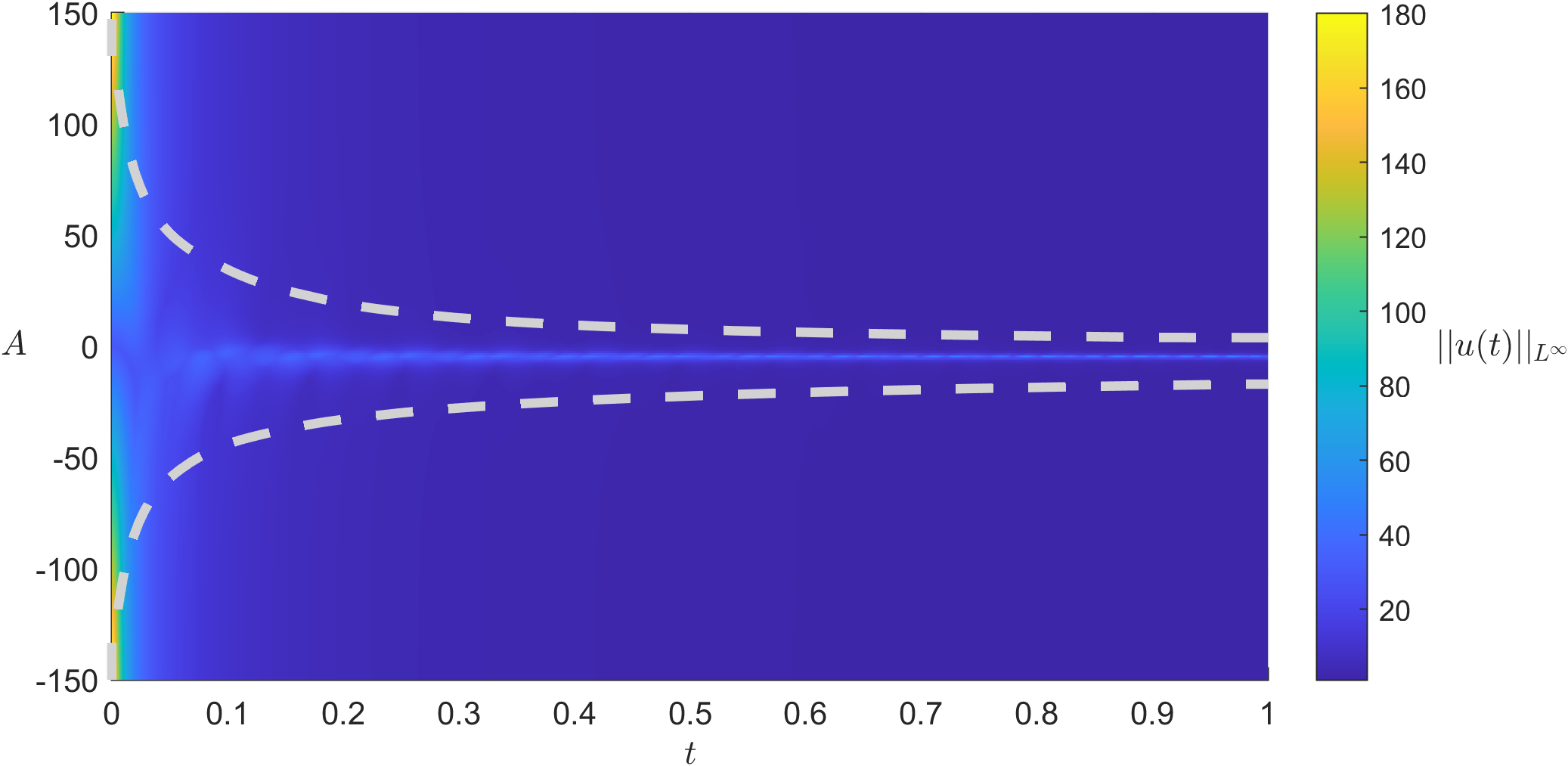
Figure 1: The norm $\|u_{30}(t;A)\|_{L^{\infty}}$ for $u_{30}(x;A)$ as in (5). The dashed gray lines represent where the solution reaches the trapping region given by Theorem 2.1.

Informed by Conjecture 1.2 we selected $A_{30}=-5.3070235$ in (5), and the solution of this initial value problem under the dynamics of the NLS (3) is plotted in Figure 2. This computation used a 4096 Fourier mode truncation and a time step of $h=10^{-7}$. We selected $A_{30}$ using a bisection method so that $u_{30}$ would be on the stable manifold $\mathcal{W}(0)$ for the nonlinear heat equation (1). We also note that nearby values of $A$ (e.g. $\approx\pm 1\%$) also appear to blowup under the dynamics of (3).

Overall, the trajectory appears to oscillate while steadily growing larger. As shown in Figure 2 (b), the $L^{\infty}$ norm of the solution maintains regular oscillations of fixed period yet steadily grows larger in amplitude. In Figure 2 (c), we display the relative composition of each Fourier modes to the $L^{2}$ norm. By Parseval’s identity $\|u(t)\|_{L^{2}}^{2}=\|a(t)\|_{\ell^{2}}=|a_{0}(t)|^{2}+2\sum_{n=1}^{\infty}|a_{n}(t)|^{2}$, and we plot in Figure 2(c) the ratio of the $n^{\text{th}}$ mode:

$$E_{n}(t):=\begin{dcases}\frac{|a_{n}|^{2}}{\|a(t)\|_{\ell^{2}}}&\mbox{if }n=0\\ \frac{2|a_{n}|^{2}}{\|a(t)\|_{\ell^{2}}}&\mbox{if }n\neq 0\end{dcases}$$ (7)

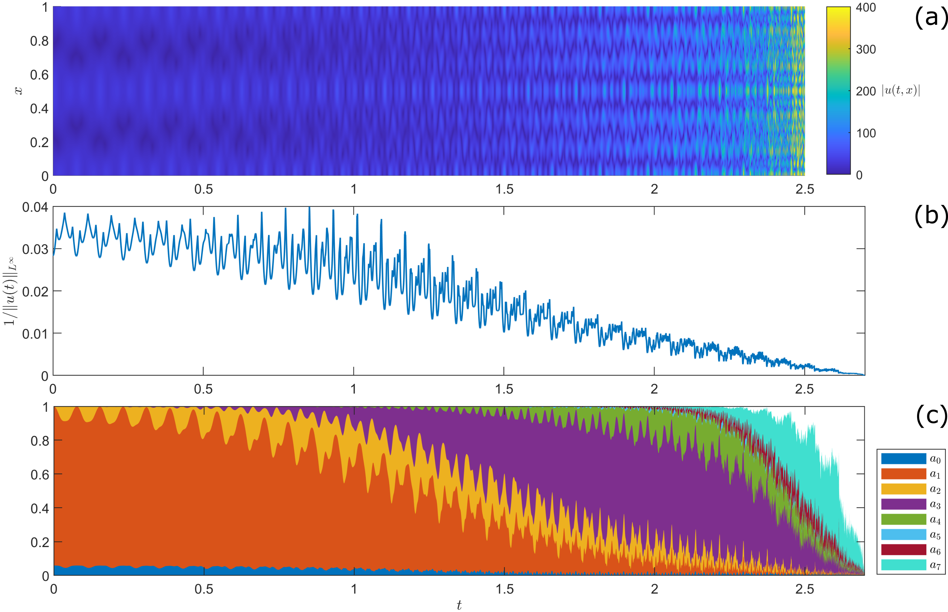
Figure 2: Solution to the NLS in (3) with initial data (5) with $A_{30}=-5.3070235$: (a) Space time plot of the solution; (b) Inverse norm of the solution $1/\|u(t)\|_{L^{\infty}}$; (c) Relative proportions $E_{n}$ of the Fourier modes, see (7).

While the spacetime plot in Figure 2(a) appears quite complex, the relative energy of each spatial mode in Figure 2(c) paints a clearer picture. As the solution evolves in time, higher spatial frequencies are progressively excited with increasing temporal oscillations. Furthermore, these oscillations grow ever more complex and almost fractal-like.

3 Secular growth of solutions along a center manifold

3.1 Dynamics of the PDE’s Galerkin truncation

To investigate the initial growth phase of the solutions we consider finite Galerkin truncations of (3). Consider a function given as a $2\pi$-periodic cosine series as in (6), where for ease of analysis in this section we take $\omega=2\pi$. Then the $N$-mode truncation of (2) yields the following dynamics on the Fourier modes:

$$e^{-i\theta}\dot{a}_{n} =-n^{2}a_{n}+\sum_{\begin{subarray}{c}n_{1}+n_{1}=n\\ -N\leq n_{1},n_{2}\leq N\end{subarray}}a_{|n_{1}|}a_{|n_{2}|}$$ (8)

By the cosine ansatz we have $a_{n}=a_{-n}$, thereby this defines a complex ODE on $\mathbb{C}^{N+1}$. Furthermore the system has an equilibrium at $0\in\mathbb{C}^{N+1}$ whose linearization has eigenvalues $\lambda_{n}=-e^{i\theta}n^{2}$ for $0\leq n\leq N$.

Define $\mathcal{W}(0)$ as the unique invariant manifold tangent to $\{0\}\times\mathbb{C}^{N}$. Selecting different values of $\theta$ will induce different internal dynamics on $\mathcal{W}$, however $\mathcal{W}$ will remain an invariant manifold for any choice of $\theta$. For example, if the real component of $-e^{i\theta}$ is negative, then $\mathcal{W}$ is a submanifold of the equilibrium’s stable set, and trajectories on $\mathcal{W}$ will exponentially approach the zero equilibrium in forward time.

More generally if $\mathcal{M}$ is an invariant complex manifold of any ODE $\dot{x}=f(x)$, then $\mathcal{M}$ will also be an invariant manifold of the system $\dot{x}=\mu f(x)$ for scalars $\mu\in\mathbb{C}$. The most well know usage of this fact is the case $\mu=-1$. That is, the stable manifold of an equilibrium in forward time is also the unstable manifold of the equilibrium in backwards time. While trajectories on $\mathcal{M}$ remain invariant when $\mu\in\mathbb{R}$, this is not the case when $\mu$ is complex.

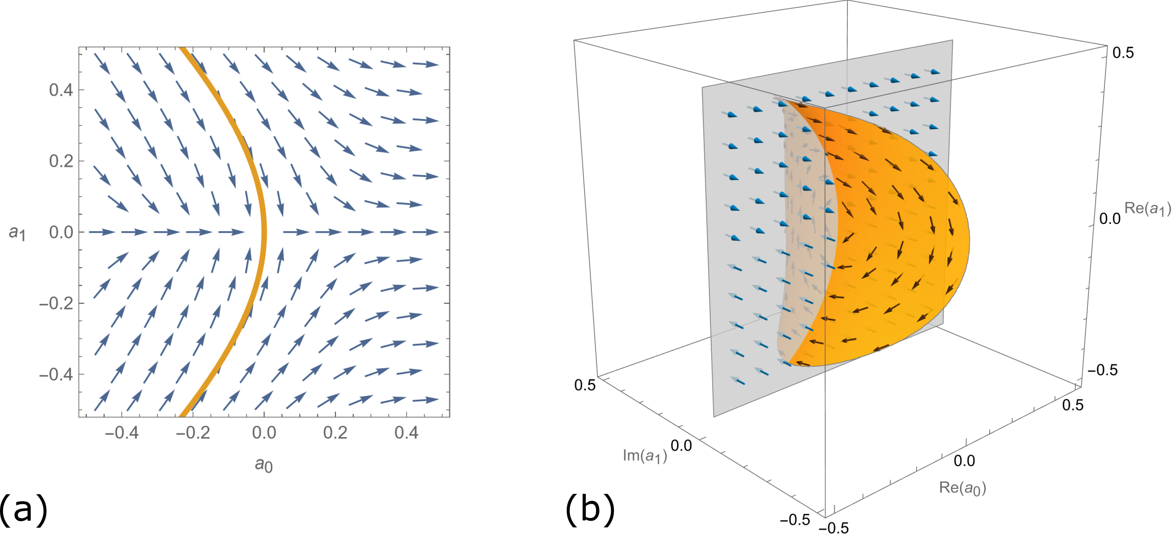
Figure 3: Phase portraits of the dynamics to (9) with the invariant manifold $\mathcal{W}$ tangent to $\{0\}\times\mathbb{C}$ depicted in orange. (a) When $\theta=0$ real initial data remains invariant, and the stable manifold $\mathcal{W}$ divides trajectories which converge to zero, from those which/that blowup in finite time. (b) When $\theta=\pi/2$, the invariant manifold $\mathcal{W}$ is foliated by periodic orbits.

For a simple illustration consider the dynamics of (8) in the case $N=1$, where we obtain the system of complex ODEs:

$$e^{-i\theta}\dot{a}_{0} =a_{0}^{2}+2a_{1}^{2}$$ (9)

$$e^{-i\theta}\dot{a}_{1} =-a_{1}+2a_{0}a_{1}$$

The case $\theta=0$ is analogous to the nonlinear heat equation (1), see Figure 3(a). Real initial data is invariant, and if $a_{0}>0$ then there is finite time blowup. Furthermore the manifold $\mathcal{W}$ divides solutions which blowup in finite time from those which converge algebraically to zero. Furthermore if $-\pi/2<\theta<\pi/2$ then solutions on $\mathcal{W}$ will exponentially decay.

In contrast, consider the case $\theta=\pm\frac{\pi}{2}$ analogous to the NLS in (3), see Figure 3(b). In this case the eigenvalues $\{\lambda_{0},\lambda_{1}\}=\{0,\mp i\}$ are purely imaginary and the manifold $\mathcal{W}$ is a submanifold of the center manifold. Furthermore $\mathcal{W}(0)$ is foliated by a Lyapunov family of periodic orbits [Hen73]. In Figure 2 we can similarly observe periodic behavior for short time scales ($0<t<0.25$). However, like with Figure 2(c), we will see in the dynamics of (8) for larger values of $N$ that there is a secular drift of solutions along $\mathcal{W}$, whereby the lower modes progressively excite the higher modes.

3.2 Parameterizing the manifold $\mathcal{W}$

The existence of stable, unstable, and center manifolds associated to equilibria has been established for a wide variety of dynamical systems, such as ODEs, PDEs, and DDEs [SY02]. However even if such a manifold is unique, its representation via a coordinate chart is not unique, nor is there just one method available for computing an approximation for the manifold.

To analyze and compute the invariant manifold $\mathcal{W}$ associated with (8) we shall use the parameterization method [CFdlL03a, CFdlL03b, CFDLL05], which has had great success analyzing the dynamics of PDEs [RJ19, JLT22a, JLT22b, GJT22, JH22, OVTF23]. This approach may be seen to be in contrast to the graph approach, where one fixes the representation of the invariant manifold as graph over the particular eigenspace and the internal dynamics need to be solved for. Instead, the parameterization method fixes the internal dynamics and solves for the coordinate chart as a map into the entire phase space.

To review the parameterization method we follow the presentation in [HCF⁺16]. Consider $F:\mathbb{C}^{n}\to\mathbb{C}^{n}$ and the differential equation given by:

$$\dot{z}=e^{i\theta}F(z)$$

having an equilibrium $z_{*}$. Let $L\in\mathbb{C}^{n\times d}$ denote a matrix whose $d$-columns are eigenvectors of the linearization $DF(z_{*})$, and let $V\subseteq\mathbb{C}^{n}$ denote the $d$-dimensional subspace spanned by the column vectors of $L$. The goal is to look for a parameterization $z=W(\sigma):\mathbb{C}^{d}\to\mathbb{C}^{n}$ of the invariant manifold $\mathcal{W}$ tangent to $V$ at $z_{*}$. The internal dynamics on the manifold are described by a vector field $\dot{\sigma}=e^{i\theta}f(\sigma)$ on $\mathbb{C}^{d}$ with $f(0)=0$, and the invariance equation is given by:

$$e^{i\theta}F(W(\sigma)) =DW(\sigma)e^{i\theta}f(\sigma)$$ (10)

Note that the complex phase $e^{i\theta}$ cancels and disappears completely!

The parameterization method seeks to write $W$ and $f$ as power series in $\sigma=(\sigma_{1},\dots,\sigma_{d})$:

$$W(\sigma) =z_{*}+\sum_{k\geq 1}W_{k}(\sigma), f(\sigma)=\sum_{k\geq 1}f_{k}(\sigma)$$ (11)

where each $W_{k}(\sigma)$ (respectively $f_{k}$) is a homogeneous polynomial in $\sigma$ of degree $k$ with coefficients in $\mathbb{C}^{n}$ (respectively with coefficients in $\mathbb{C}^{d}$), that is:

$$W_{k}(\sigma) =\sum_{k_{1}+\dots+k_{d}=k}W_{(k_{1}\dots k_{d})}\sigma_{1}^{k_{1}}\cdots\sigma_{d}^{k_{d}}, W_{(k_{1}\dots k_{d})} \in\mathbb{C}^{n}$$ (12)

To enforce the invariant manifold $\mathcal{W}$ being tangent to the eigenspace $V$ we take $W_{1}(\sigma)=L\sigma$ and $f_{1}(\sigma)=\Lambda_{L}\sigma$. The higher order terms in the power series may be obtained by matching the order-$k$ terms in (10), yielding the cohomological equations:

$$DF(z_{*})W_{k}(\sigma)-DW_{k}(\sigma)\Lambda_{L}\sigma-Lf_{k}(\sigma)=-E_{k}(\sigma)$$ (13)

where:

$$E_{k}(\sigma)=[F(W_{<k}(\sigma))]_{k}-[DW_{<k}(\sigma)f_{<k}(\sigma)]_{k}$$

is the order-$k$ error term, depending only on coefficients whose order is strictly less that $k$. Thus through (13) the coefficients $W_{k}$ may be solved recursively for orders $k\geq 2$, subject to the choice of coefficients $f_{k}$.

The simplest dynamics one may conjugate to is linear dynamics $\dot{\sigma}=\Lambda_{L}\sigma$ wherein $f_{k}=0$ for $k\geq 2$. Then for each $\vec{k}=(k_{1},\dots,k_{d})$ equation (13) reduces to the linear system:

$$(DF(z_{*})-\vec{k}\cdot\lambda I_{n})W_{\vec{k}}=-E_{\vec{k}}$$

This can be solved for $|k|\geq 2$ so long as the matrix $(DF(z_{*})-\vec{k}\cdot\lambda I_{n})$ is invertible. This fails to occur when there is an internal resonance, which is to say when:

$$\vec{k}\cdot\lambda=\lambda_{i}$$

for $\vec{k}\in\mathbb{N}^{d}$ and $|k|\geq 2$. This can only occur if the eigenvalues $(\lambda_{1}\dots\lambda_{d})$ are rationally dependent.

Returning to the dynamics resulting from the Galerkin truncation in (8), recall that the zero equilibrium has eigenvalues $\lambda_{n}=-e^{i\theta}n^{2}$ for integers $0\leq n\leq N$. Thus, resonances occur whenever we can write a square integer as a sum of other square integers:

$$m^{2}=\sum_{n=1}^{m-1}k_{n}n^{2}$$

for non-negative integers $k_{n}$ with $k_{1}+\dots+k_{m-1}\geq 2$. This happens abundantly often! For example $m^{2}=m^{2}\cdot 1^{2}$ or $m^{2}=(m^{2}-n^{2})\cdot 1^{2}+1\cdot n^{2}$ for any $1<n<m$. While resonances are an obstruction to conjugating the internal dynamics of $\mathcal{W}$ to a linear system, a parameterization may still be obtained for more nontrivial internal dynamics.

For an example, consider the $N=3$ Galerkin truncation of (8) given by:

$$e^{-i\theta}\dot{a}_{0} =a_{0}^{2}+2a_{1}^{2}+2a_{2}^{2}+2a_{3}^{2}$$

$$e^{-i\theta}\dot{a}_{1} =-a_{1}+2a_{0}a_{1}+2a_{1}a_{2}+2a_{2}a_{3}$$ (14)

$$e^{-i\theta}\dot{a}_{2} =-4a_{2}+2a_{0}a_{2}+a_{1}^{2}+2a_{1}a_{3}$$

$$e^{-i\theta}\dot{a}_{3} =-9a_{3}+2a_{0}a_{3}+2a_{1}a_{2}$$

Again, we define $\mathcal{W}(0)$ as the unique invariant manifold tangent to $\{0\}\times\mathbb{C}^{3}$. The equilibrium’s nonzero eigenvalues are $e^{-i\theta}\lambda=(-1,-4,-9)$, and we obtain the resonances:

$$(4,0,0)\cdot\lambda =\lambda_{2}, (1,2,0)\cdot\lambda =\lambda_{3}, (5,1,0)\cdot\lambda =\lambda_{3}, (9,0,0)\cdot\lambda =\lambda_{3}$$

One can deal with resonances by adjusting the function $f$, that one conjugates the dynamics to [vdBMJR16]. In our code [Jaq24] we calculate a parameterization $W$ such that the dynamics are conjugate to:

$$\mu^{-1}\dot{\sigma}_{1} =-\sigma_{1}$$

$$\mu^{-1}\dot{\sigma}_{2} =-4\sigma_{2}+\tfrac{1}{3}\sigma_{1}^{4}$$ (15)

$$\mu^{-1}\dot{\sigma}_{3} =-9\sigma_{3}-\sigma_{1}\sigma_{2}^{2}+\tfrac{19}{24}\sigma_{1}^{5}\sigma_{2}+\tfrac{11}{81}\sigma_{1}^{9}$$

where $\mu=e^{i\theta}$. The specific coefficients for the higher order terms, such as $\frac{1}{3}\sigma_{1}^{4}$ and $\tfrac{19}{24}\sigma_{1}^{5}\sigma_{2}$, are not able to be determined in advance and requires one to first solve the cohomological equation (13) for all of the lower order terms. While nonlinear, the internal dynamics of $\mathcal{W}$ determined by (15) is integrable, and for initial data $\sigma(0)=(\gamma_{1},\gamma_{2},\gamma_{3})$ its solution is given by:

$$\sigma_{1}(t) =\gamma_{1}e^{-\mu t},$$

$$\sigma_{2}(t) =\left(\gamma_{2}+\frac{\mu t}{3}\gamma_{1}^{4}\right)e^{-4\mu t},$$ (16)

$$\sigma_{3}(t) =\left(\gamma_{3}-\mu t\gamma_{1}\gamma_{2}^{2}+\left(\frac{19\mu t}{24}-\frac{\mu^{2}t^{2}}{3}\right)\gamma_{1}^{5}\gamma_{2}+\left(\frac{11\mu t}{81}+\frac{19\mu^{2}t^{2}}{144}-\frac{\mu^{3}t^{3}}{27}\right)\gamma_{1}^{9}\right)e^{-9\mu t}$$

Note that if $-\pi/2<\theta<\pi/2$ then $Re(-\mu)<0$ whereby all of these solutions exponentially decay.

However if $\theta=\pm\pi/2$ then $\mu=\pm i$, whereby the solutions in (16) are oscillatory with secular drift exciting the higher modes. Indeed, while $|\sigma_{1}(t)|$ stays bounded for all $t$, the higher modes grow like $|\sigma_{2}(t)|=\mathcal{O}(t|\gamma_{1}|^{4})$ and $|\sigma_{3}(t)|=\mathcal{O}(t^{3}|\gamma_{1}|^{9})$. Hence small initial data in the lowest modes requires a long time before the higher modes are excited to a comparable level.

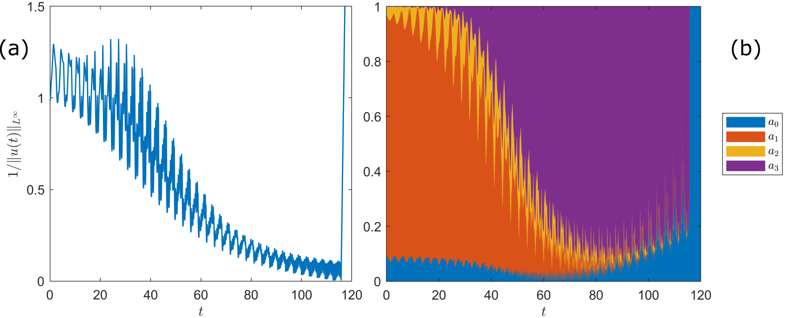
Figure 4: Solution to the four-mode Galerkin truncation in (3.2) with initial data (17) (a): The inverse norm $1/\|u^{(N)}(t)\|_{L^{\infty}}$ ; (b) Relative proportions $E_{n}$ of the Fourier modes, see (7).

Like with any power series, the parameterization of $\mathcal{W}$ is only valid on the power series’ radius of convergence. (Based on our computation, the radius of convergence seems to be about $0.80$.) While the explicit solutions given in (16) never blow up, it may be possible for a solution on $\mathcal{W}$ to blowup after it leaves the local coordinate chart. To investigate this, we consider the following initial condition selected on the invariant manifold $\mathcal{W}$:

$$\left(\begin{matrix}\sigma_{1}\\ \sigma_{2}\\ \sigma_{3}\end{matrix}\right) =\left(\begin{matrix}\;0.4300654917290795\\ -0.07398732057014827\\ \;\;0.00530826265454094\end{matrix}\right), W(\sigma) =\left(\begin{matrix}-0.22301409257004942\\ 0.5\\ 0\\ 0\end{matrix}\right)$$ (17)

When integrated under (3.2) with $\theta=\pi/2$ this trajectory undergoes a large growth in norm, see Figure 4. Like with Figure 2, one can see that there is a steady cascade pumping energy into the higher modes. This initial condition does not appear to completely blowup, as in the later stage of trajectory $1/\|u(t)\|_{L^{\infty}}$ grows rapidly. However, such a non-blowup may also be seen to be consistent with the existence of an unstable blowup profile. Note also that as our computation of $\mathcal{W}$ was with a finite Taylor series, our the initial condition was not exactly on the manifold $\mathcal{W}$. (For our 20th order Taylor approximation of $W$, we estimate the error of the initial point to be on the order of $10^{-5}$.) While one could get a more precise initial point on the manifold by choosing a smaller initial condition $\sigma$, this would conversely increase the integration time and the associated errors.

4 Apparent self-similar blowup profiles

The finite Fourier truncation model offers a heuristic explanation for why initial data from the stable manifold of the heat equation (1) will grow larger, and exhibit a seemingly periodic forward cascade to the higher modes. However this analysis is localized at the zero equilibrium. While it is suggestive of how small initial data grows to become finitely large in norm, it does not explain how large initial data may grow without bound and blowup.

To focus on the dynamics of blowup we consider larger initial data. With consideration to Conjecture 1.2, we fix the following real initial data:

$$u_{300}(x) =300\cos(2\pi x)+A_{300}, A_{300} =-189.286840601635,$$ (18)

see Figure 5. We used computational parameters of 4096 Fourier mode truncation and a time step of $h=10^{-7}$. For comparison we also consider monochromatic initial data:

$$u_{300}^{mc}(x) =300e^{2\pi ix},$$ (19)

see Figure 6. As $300>6(2\pi)^{2}\approx 236.9$, the initial data in (19) is guaranteed to blowup as per [Jaq22].

Theorem 4.1 (Theorem 1.5[Jaq22]).

Consider (3) with initial data $u_{0}(x)=Ae^{i\omega x}$ with $A\in\mathbb{C}$, $\omega>0$.

1. If $|A|\leq 3\omega^{2}$, then $u$ is a smooth periodic solution with period $\frac{2\pi}{\omega^{2}}$.

2. If $|A|\geq 6\omega^{2}$, then $\|u(t)\|_{L^{2}}$ blows up in finite time $|T_{*}|\leq\frac{2\pi}{\omega^{2}}$.

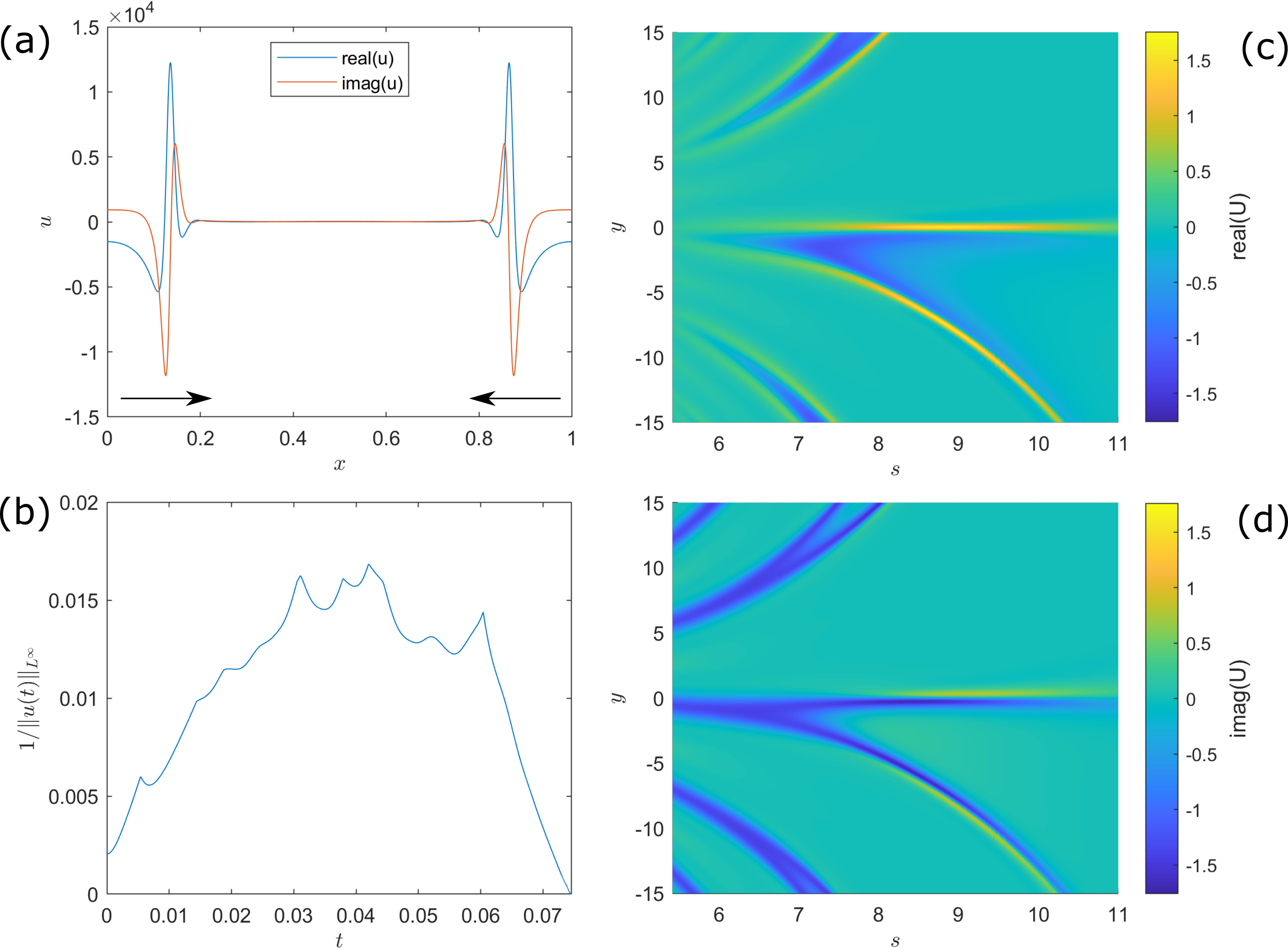
Figure 5: Numerical solution of (3) using initial data from (18). (a) Real and imaginary components of $u(t,x)$ when $t=0.0743$ ($s=8.95$), depicted with the direction of movement of the blowup point(s); (b) Inverse norm of solution $1/\|u(t)\|_{L^{\infty}}$; (c-d) Real and imaginary components of $U$ from (20) using self-similar coordinates with scaling $(\alpha,\beta)=(1,1/2)$.

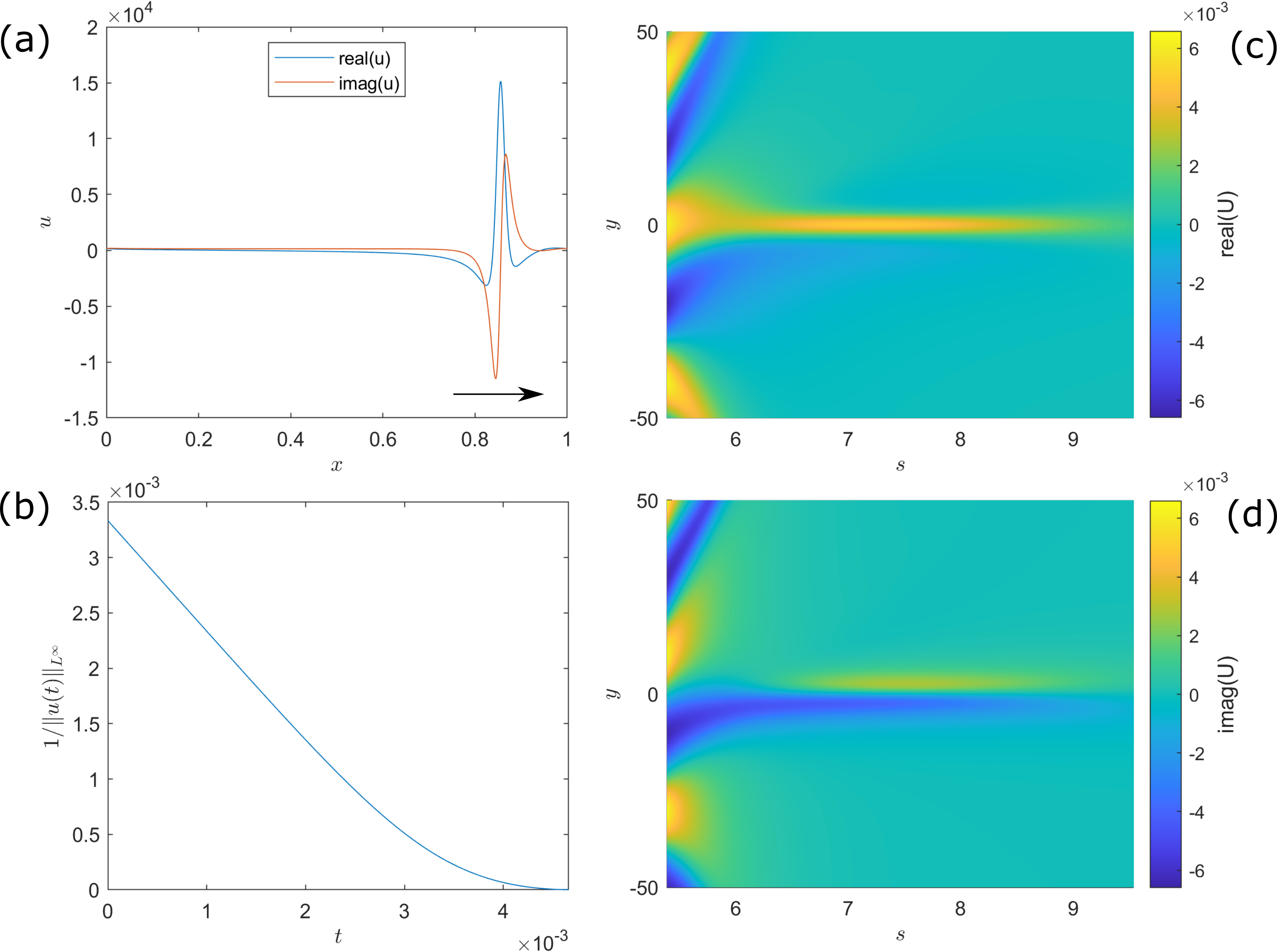
Figure 6: Numerical solution of (3) using initial data from (19). (a) Real and imaginary components of $u(t,x)$ when $t=0.004$ ($s=7.47$), depicted with the direction of movement of the blowup point; (b) Inverse norm of solution $1/\|u(t)\|_{L^{\infty}}$; (c-d) Real and imaginary components of $U$ from (20) using self-similar coordinates with scaling $(\alpha,\beta)=(2,1)$.

As predicted by Conjecture 1.2 and Theorem 4.1, the numerical solutions of the initial data (18) and (19) appear to blowup. Plotted in Figures 5-6(a) are the numerical solutions after a period of time. While the monochromatic initial data yields a single blowup point moving to the right, the real initial data produces two blowup points moving in opposite directions.

Moreover, the solutions appear to undergo self-similar blowup. In a general context, this occurs when a blowup solution $u$ to a given PDE can be regularized using a self-similar change of variables into a new solution $U$ with nontrivial limiting behavior [EF08, QS19]. For a given blowup time $T$ and pair of scaling parameters $(\alpha,\beta)$ define:

$$u(t,x) =\frac{1}{(T-t)^{\alpha}}U(s,y)$$ (20)

using the self-similar coordinates:

$$y =\frac{x-\xi(t)}{(T-t)^{\beta}} s =-\log(T-t)$$ (21)

where $\xi(t)$ denotes the moving location of the spatial blowup point. Note that if $\alpha>0$ and $\liminf_{s\to\infty}\|U(s)\|_{L^{\infty}}>0$, then $u(t)$ blows up as $t\to T$. While the dynamics of $u$ are singular as $t\to T$, ideally the dynamics of $U$ are well behaved as $s\to\infty$.

In Figures 5-6(b) the inverse norm $1/\|u(t)\|_{L^{\infty}}$ can be seen to approach zero (thus blowing up). The solution with real initial data first decreases in norm and oscillates to a small extent before it begins a path towards blowup. In contrast, the solution with monochromatic initial data immediately increases in norm and accelerates in the later stage.

To estimate the scaling parameter $\alpha$, we fit the data in Figures 5-6(b) to the equation $y(t)=C_{0}|T-t|^{\alpha}$. For the solution with real initial data, fitting the data over the time interval $[0.070,0.074]$ yielded $\alpha=1.1457$ with an $R^{2}$ value of $0.9999$. For the solution with monochromatic initial data, fitting the data over the time interval $[0.038,0.045]$ yielded $\alpha=2.0098$ with an $R^{2}$ value of $0.9992$. Note that even though the two blowup profiles in Figures 5-6(a) look qualitatively similar, they appear to obey distinct rates of blowup. Additionally, while the $R^{2}$ values are suggestive of a good fit, the residual errors are not normally distributed, indicative of systematic bias. Practically speaking, we observe that fit parameters are quite sensitive to the time range over which the data is fit. For the case of real initial data, the non-integer value of $\alpha$ may also be suggestive of a logarithmic correction term being needed in the norm scaling, as is the case with the nonlinear heat equation [BK94, MZ97].

To investigate whether these numerical solutions obey self-similar scaling, we perform a change of variables in (3) using the self-similar coordinates, resulting in the following equations that govern the self-similar dynamics:

$$i\left(\alpha U+\partial_{s}U+\beta y\partial_{y}U\right) =e^{(2\beta-1)s}\partial_{yy}U+e^{(\beta-1)s}i\dot{\xi}\partial_{y}U+e^{(\alpha-1)s}U^{2}$$ (22)

For consistency in scaling, balance laws suggest that $\alpha=2\beta$. Rounding to the closest integer our statistical fits for $\alpha$, we obtain scaling parameters $(\alpha,\beta)=(1,1/2)$ for the real initial data and $(\alpha,\beta)=(2,1)$ for the monochromatic initial data. Making the change of variables into these self-similar coordinates, we plot the solutions $U(s,y)$ in Figure 5-6(c-d) for the real and imaginary components of the solutions.

In Figure 5-6(c-d) the self-similar solutions $U(s,y)$ appear to be decently regularized. For smaller values of $s$, periodic copies of the blowup profile may be observed to diverge away from $y=0$, as would be expected. For larger values of $s$ however the blowup profile appears to fade, a likely result of an imprecise selection of the blowup time, and the significant numerical error which accumulate as the blowup time is approached. While the solution with real initial data appears to grow according to a power law starting at $t\geq 0.06$, the blowup profile qualitatively changes. This may be most prominently seen in Figure 5(d) when comparing the imaginary component of $U(s,y)$ over the regions $s\in[6,7]$ and $s\in[8,10]$, and may be indicative of non-trivial self-similar dynamics.

Alternatively, the simplest blowup scenario would be the so-called Type-I blowup [EF08, QS19], whereby $U$ converges to an equilibrium with scaling parameters $(\alpha,\beta)=(1,1/2)$ and (22) simplifies to:

$$i\left(U+\partial_{s}U+\tfrac{y}{2}\partial_{y}U\right) =\partial_{yy}U+e^{-s/2}i\dot{\xi}\partial_{y}U+U^{2}$$ (23)

In this case, as $\lim_{s\to\infty}e^{-s/2}=0$, an equilibrium solution would satisfy the following second order ODE:

$$0 =\partial_{yy}U-\tfrac{i}{2}y\partial_{y}U-iU+U^{2}, \lim_{y\to\pm\infty}|U(y)|=0$$ (24)

Despite our efforts, we have not found a nontrivial solution to (24).

5 Conclusion

While Conjecture 1.1 may be true in a generic sense, we have presented numerical evidence of real initial data to (3) which blows up in finite time. By tracking solutions to the 1-parameter family of initial data in (5), we were able to identify initial conditions leading to blowup. While tracking the $L^{\infty}$ norm of solutions proved sufficient, measuring when solutions entered a trapping region of zero provided a much more robust method of identification.

As previously mentioned, the blowup solution identified in Section 2 has two distinct qualitative features: (i) on shorter time scales, the solution periodic oscillates with progressive excitement of the higher modes; (ii) on longer time scales, the solution steadily grows, eventually leading to blowup. In Section 3 we provide a heuristic explanation for the mechanisms behind feature (i). Namely, we use the parameterization method to analyze a submanifold $\mathcal{W}$ of the center manifold of $0$. While solutions on $\mathcal{W}$ do oscillate, a secular drift due to a resonance of eigenvalues induces a cascade whereby the lower modes excite the higher modes.

This analysis leads us to propose Conjecture 1.2, that real initial data to (3) will blowup if and only if it lies on the stable manifold of $0$ for the nonlinear heat equation (1). We note that the finite Galerkin truncation model only has a finite number of eigenvalue resonances, and is thus amenable to the parameterization method. While empirical evidence supports Conjecture 1.2, we cannot hope to prove it using the parameterization method due to the infinite number of resonances in the full PDE.

To analyze the later stage of blowup in (3) we performed a self-similar analysis in Section 4, comparing blowup solutions starting from both real and monochromatic initial data. While both solutions appear to exhibit self-similar blowup, key questions remain. For example, what is the exact scaling rate for the solution starting with real initial data, and is a logarithmic correction term required? And does the self-similar solution limit to an equilibrium or some more complicated dynamical object, such as a periodic orbit or a chaotic attractor?

References

- [BK94] Jean Bricmont and Antti Kupiainen. Universality in blow-up for nonlinear heat equations. Nonlinearity, 7(2):539, 1994.
- [CFdlL03a] Xavier Cabré, Ernest Fontich, and Rafael de la Llave. The parameterization method for invariant manifolds I: manifolds associated to non-resonant subspaces. Indiana University mathematics journal, pages 283–328, 2003.
- [CFdlL03b] Xavier Cabré, Ernest Fontich, and Rafael de la Llave. The parameterization method for invariant manifolds II: regularity with respect to parameters. Indiana University mathematics journal, pages 329–360, 2003.
- [CFDLL05] Xavier Cabré, Ernest Fontich, and Rafael De La Llave. The parameterization method for invariant manifolds III: overview and applications. Journal of Differential Equations, 218(2):444–515, 2005.
- [CLM85] Peter Constantin, Peter D Lax, and Andrew Majda. A simple one-dimensional model for the three-dimensional vorticity equation. Communications on pure and applied mathematics, 38(6):715–724, 1985.
- [CM18] Ciro S Campolina and Alexei A Mailybaev. Chaotic blowup in the 3d incompressible Euler equations on a logarithmic lattice. Physical review letters, 121(6):064501, 2018.
- [COS16] C.-H. Cho, H. Okamoto, and M. Shōji. A blow-up problem for a nonlinear heat equation in the complex plane of time. Japan Journal of Industrial and Applied Mathematics, 33(1):145–166, Feb 2016.
- [DHT14] Tobin A Driscoll, Nicholas Hale, and Lloyd N Trefethen. Chebfun guide, 2014.
- [EF08] Jens Eggers and Marco A Fontelos. The role of self-similarity in singularities of partial differential equations. Nonlinearity, 22(1):R1, 2008.
- [Fef00] Charles L Fefferman. Existence and smoothness of the Navier-stokes equation. The millennium prize problems, 57:67, 2000.
- [FMS23] Yue Feng, Georg Maierhofer, and Katharina Schratz. Long-time error bounds of low-regularity integrators for nonlinear Schrödinger equations. arXiv preprint arXiv:2302.00383, 2023.
- [FS24] Bernold Fiedler and Hannes Stuke. Real eternal PDE solutions are not complex entire: a quadratic parabolic example. arXiv preprint arXiv:2403.06490, 2024.
- [GJT22] Jorge Gonzalez, JD Mireles James, and Necibe Tuncer. Finite element approximation of invariant manifolds by the parameterization method. Partial Differential Equations and Applications, 3(6):75, 2022.
- [GNSY13] Jong-Shenq Guo, Hirokazu Ninomiya, Masahiko Shimojo, and Eiji Yanagida. Convergence and blow-up of solutions for a complex-valued heat equation with a quadratic nonlinearity. Transactions of the American Mathematical Society, 365(5):2447–2467, 2013.
- [HCF+16] Alex Haro, Marta Canadell, Jordi-Lluis Figueras, Alejandro Luque, and Josep-Maria Mondelo. The parameterization method for invariant manifolds. Applied mathematical sciences, 195, 2016.
- [Hen73] Jacques Henrard. Lyapunov’s center theorem for resonant equilibrium. Journal of Differential Equations, 14(3):431–441, 1973.
- [HL08] Thomas Y Hou and Congming Li. Dynamic stability of the three-dimensional axisymmetric Navier-Stokes equations with swirl. Communications on Pure and Applied Mathematics: A Journal Issued by the Courant Institute of Mathematical Sciences, 61(5):661–697, 2008.
- [Hou23] Thomas Y Hou. Potentially singular behavior of the 3d Navier–Stokes equations. Foundations of Computational Mathematics, 23(6):2251–2299, 2023.
- [Jaq22] Jonathan Jaquette. Quasiperiodicity and blowup in integrable subsystems of nonconservative nonlinear Schrödinger equations. Journal of Dynamics and Differential Equations, pages 1–25, 2022.
- [Jaq24] Jonathan Jaquette. Matlab code of “Mechanisms of unstable blowup in a quadratic nonlinear Schrödinger equation”. https://github.com/JCJaquette/Unstable-Blowup-NLS, 2024.
- [JH22] Shobhit Jain and George Haller. How to compute invariant manifolds and their reduced dynamics in high-dimensional finite element models. Nonlinear dynamics, 107(2):1417–1450, 2022.
- [JLT22a] Jonathan Jaquette, Jean-Philippe Lessard, and Akitoshi Takayasu. Global dynamics in nonconservative nonlinear Schrödinger equations. Advances in Mathematics, 398:108234, 2022.
- [JLT22b] Jonathan Jaquette, Jean-Philippe Lessard, and Akitoshi Takayasu. Singularities and heteroclinic connections in complex-valued evolutionary equations with a quadratic nonlinearity. Communications in Nonlinear Science and Numerical Simulation, 107:106188, 2022.
- [Mas83] Kyûya Masuda. Blow-up of solutions of some nonlinear diffusion equations. In Hiroshi Fujita, Peter D. Lax, and Gilbert Strang, editors, Nonlinear Partial Differential Equations in Applied Science; Proceedings of The U.S.-Japan Seminar, Tokyo, 1982, volume 81 of North-Holland Mathematics Studies, pages 119 – 131. North-Holland, 1983.
- [Mas84] Kyûya Masuda. Analytic solutions of some nonlinear diffusion equations. Mathematische Zeitschrift, 187(1):61–73, Mar 1984.
- [MZ97] Frank Merle and Hatem Zaag. Stability of the blow-up profile for equations of the type . Duke Mathematical Journal, 86(1):143 – 195, 1997.
- [OVTF23] Andrea Opreni, Alessandra Vizzaccaro, Cyril Touzé, and Attilio Frangi. High-order direct parametrisation of invariant manifolds for model order reduction of finite element structures: application to generic forcing terms and parametrically excited systems. Nonlinear Dynamics, 111(6):5401–5447, 2023.
- [Pro22] Bartosz Protas. Systematic search for extreme and singular behaviour in some fundamental models of fluid mechanics. Philosophical Transactions of the Royal Society A, 380(2225):20210035, 2022.
- [QS19] Pavol Quittner and Philippe Souplet. Superlinear parabolic problems. Springer, 2019.
- [RJ19] Christian Reinhardt and JD Mireles James. Fourier–Taylor parameterization of unstable manifolds for parabolic partial differential equations: Formalism, implementation and rigorous validation. Indagationes Mathematicae, 30(1):39–80, 2019.
- [SY02] George R Sell and Yuncheng You. Dynamics of evolutionary equations, volume 143. Springer Science & Business Media, 2002.
- [vdBMJR16] Jan Bouwe van den Berg, Jason D Mireles James, and Christian Reinhardt. Computing (un) stable manifolds with validated error bounds: non-resonant and resonant spectra. Journal of Nonlinear Science, 26:1055–1095, 2016.
- [WLGSB23] Yongji Wang, C-Y Lai, Javier Gómez-Serrano, and Tristan Buckmaster. Asymptotic self-similar blow-up profile for three-dimensional axisymmetric Euler equations using neural networks. Physical Review Letters, 130(24):244002, 2023.