Full-Atom Peptide Design based on Multi-modal Flow Matching

Abstract

Peptides, short chains of amino acid residues, play a vital role in numerous biological processes by interacting with other target molecules, offering substantial potential in drug discovery. In this work, we present PepFlow, the first multi-modal deep generative model grounded in the flow-matching framework for the design of full-atom peptides that target specific protein receptors. Drawing inspiration from the crucial roles of residue backbone orientations and side-chain dynamics in protein-peptide interactions, we characterize the peptide structure using rigid backbone frames within the $\mathrm{SE}(3)$ manifold and side-chain angles on high-dimensional tori. Furthermore, we represent discrete residue types in the peptide sequence as categorical distributions on the probability simplex. By learning the joint distributions of each modality using derived flows and vector fields on corresponding manifolds, our method excels in the fine-grained design of full-atom peptides. Harnessing the multi-modal paradigm, our approach adeptly tackles various tasks such as fix-backbone sequence design and side-chain packing through partial sampling. Through meticulously crafted experiments, we demonstrate that PepFlow exhibits superior performance in comprehensive benchmarks, highlighting its significant potential in computational peptide design and analysis.

1 Introduction

Peptides, comprising approximately $3$ to $20$ amino-acid residues, are single-chain proteins (Bodanszky, 1988). By binding to other molecules, especially target proteins (receptors), peptides serve as integral players in diverse biological processes, such as cellular signaling, enzymatic catalysis, and immune responses (Petsalaki & Russell, 2008; Kaspar & Reichert, 2013). Therapeutic peptides that bind to diseases-associated proteins are gaining recognition as promising drug candidates due to their strong affinity, low toxicity, and easy delivery (Craik et al., 2013; Fosgerau & Hoffmann, 2015; Muttenthaler et al., 2021; Wang et al., 2022). Traditional discovery methods, such as mutagenesis and immunization-based library construction, face limitations due to the vast design space of peptides (Lam, 1997; Vlieghe et al., 2010; Fosgerau & Hoffmann, 2015). To break the experimental constraints, there is a growing demand for computational methods facilitating in silico peptide design and analysis (Bhardwaj et al., 2016; Cao et al., 2022; Xie et al., 2023; Manshour et al., 2023; Bryant & Elofsson, 2023; Bhat et al., 2023).

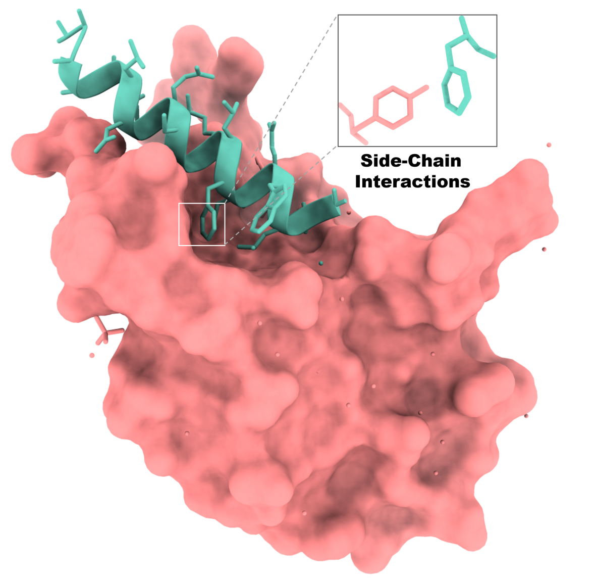
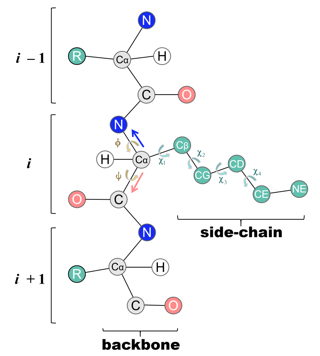
Figure 1: Left. A peptide binds to its target protein receptor, highlighting the pivotal role of backbone orientations and side-chain interactions among key residues. Right. Every protein residue consists of backbone atoms and side-chain atoms. The backbone atoms establish a rigid frame, whereas the side-chain atoms contribute to flexible side-chain angles.

Recently, deep generative models, particularly diffusion probabilistic models (Sohl-Dickstein et al., 2015; Ho et al., 2020; Song & Ermon, 2019; Song et al., 2020b), have shown considerable promise in de novo protein design (Huang et al., 2016). These models mainly focus on generating protein backbones, represented as $N$ rigid frames in the $\mathrm{SE}(3)$ manifold (Trippe et al., 2022; Anand & Achim, 2022; Luo et al., 2022; Wu et al., 2022; Ingraham et al., 2023; Yim et al., 2023b). The current state-of-the-art method, RFDiffusion (Watson et al., 2022) excels in designing a diverse array of functional proteins with an enhanced success rate validated through experiments (Roel-Touris et al., 2023).

Though achieving remarkable success in protein backbone design, current generative models still encounter challenges in generating peptide binders conditioned on a specific target protein (Bennett et al., 2023). Unlike unconditional generation, generating binding peptides necessitates explicit conditioning on binding pockets, as the bound-state structures of peptides in protein-peptide complexes partially depend on their targets (Duffaud et al., 1985; Dagliyan et al., 2011) and peptides contact accurate binding sites for biological functions. Furthermore, as shown in Figure 1, in protein-peptide interactions (Stanfield & Wilson, 1995; Jacobson et al., 2002), the focus should extend beyond the positions and orientations of the backbones to encompass the dynamics of side-chain angles, where residues interact with each other through non-covalent forces formed by side-chain groups. Consequently, peptide generation should consider full-atom structures rather than solely concentrating on modeling the four backbone heavy atoms. Also, since the structure of the functional peptide is mainly determined by its sequence (Whisstock & Lesk, 2003), it is essential to simultaneously consider sequence and structure during generation to enhance consistency between them.

To address the challenges mentioned above, we introduce PepFlow, a multi-modal deep generative model built upon the Conditional Flow Matching (CFM) framework (Lipman et al., 2022). CFM learns the continuous normalizing flow (Chen et al., 2018) by regressing the vector field that transforms prior distributions to target distributions. It has demonstrated competitive generation performance compared to the diffusion framework and is handy to adopt on non-Euclidean manifolds (Chen & Lipman, 2023). We further extend CFM to modalities related to full-atom proteins. In our framework, each residue in the peptide is represented as a rigid frame in $\mathrm{SE}(3)$ for backbone, a point on a hypertorus corresponding to side-chain angles, and an element on the probability simplex indicating the discrete type. We derive analytical flows for each modality and model the joint distribution of the full-atom peptide structure and sequence conditioned on the target protein. Subsequently, we can design full-atom peptides by simultaneously transforming from the prior distribution to the learned distribution on each modality. Our method extends its applicability to other tasks including fix-backbone sequence design and side-chain packing, which is achieved through partial sampling for desired modalities. Notably, there is no current comprehensive benchmark for evaluating generative models in peptide design, we further introduce a new dataset with in-depth metrics to quantify the qualities of generated peptides.

In summary, our key contributions include:

• We introduce PepFlow, the first multi-modal generative model for designing full-atom protein structures and sequences

• We pioneer the resolution of challenges in target-specific peptide design and establish comprehensive benchmarks, including newly cleaned dataset and novel in silico metrics to evaluate generated peptides.

• Our method showcases superior performance and great scalability across a spectrum of peptide design and analysis tasks encompassing sequence-structure co-design, fix-backbone sequence design, and side-chain packing.

2 Related Work

Diffusion-based and Flow-based Generative Models Trained on the denoising score matching objective (Vincent, 2011), diffusion models refine samples from prior Gaussian distributions into gradually meaningful outputs (Sohl-Dickstein et al., 2015; Ho et al., 2020; Song & Ermon, 2019; Song et al., 2020b). Diffusion models are applicable in diverse modalities, e.g. images (Ho et al., 2020; Zhang et al., 2023a), texts (Austin et al., 2021; Hoogeboom et al., 2021) and molecules (Hoogeboom et al., 2022; Xu et al., 2022; Jing et al., 2022). However, they rely on stochastic estimation which leads to suboptimal probability paths and longer sample steps (Song et al., 2020a; Lu et al., 2022).

Another direction considers ODE-based continuous normalizing flows as an alternative to diffusion models (Chen et al., 2018). Conditional Flow Matching (CFM) (Lipman et al., 2022; Liu et al., 2022; Albergo & Vanden-Eijnden, 2022) directly learns the ODE that traces the probability path from the prior distribution to the target, regressing the pushing-forward vector field conditioned on individual data points. Additionally, Riemannian Flow Matching (Chen & Lipman, 2023) extends CFM to general manifolds without the requirement for expensive simulations (Ben-Hamu et al., 2022; De Bortoli et al., 2022; Huang et al., 2022). In our work, we use the flow matching framework to conditionally model full-atom structures and sequences of peptide binders. Though previous work existed in applying flow matching models in molecular generation (Song et al., 2023; Bose et al., 2023; Yim et al., 2023a, 2024), they mainly focused on specific modalities or unconditional generation.

De novo Protein Design with Generative Models Generative models have demonstrated promising performance in the design of protein-related applications including enzyme active sites (Yeh et al., 2023; Dauparas et al., 2023; Zhang et al., 2023c) and motif scaffolds (Wang et al., 2021; Trippe et al., 2022; Yim et al., 2024). These methods can be categorized into three main schemes: sequence design, structure design, and sequence-structure co-design. In sequence design, protein sequences are crafted using oracle-based directed evolution (Jain et al., 2022; Ren et al., 2022; Khan et al., 2022; Stanton et al., 2022), protein language models (Madani et al., 2020; Verkuil et al., 2022; Nijkamp et al., 2023), and discrete diffusion models (Alamdari et al., 2023; Frey et al., 2023; Gruver et al., 2024; Yi et al., 2024).Alternatively, sequences are sampled based on protein backbone structures, known as fix-backbone sequence design (Ingraham et al., 2019; Jing et al., 2020; Hsu et al., 2022; Li et al., 2022; Gao et al., 2022). Recognizing the important role of protein 3D structures, another approach involves directly generating protein backbone structures (Trippe et al., 2022; Anand & Achim, 2022; Luo et al., 2022; Wu et al., 2022; Ingraham et al., 2023). These backbones are then fed into fix-backbone design models to predict the corresponding sequences, e.g. ProteinMPNN (Dauparas et al., 2022). Sequence-structure co-design methods jointly sample sequence-structure pairs conditioned on provided information and find widespread usage in designing antibodies (Jin et al., 2021; Luo et al., 2022; Kong et al., 2022). Nevertheless, few methods focus on the interplay of side-chain interactions in the conditional generation of proteins or concurrently producing protein structures and sequences in full atomic detail (Martinkus et al., 2023; Kong et al., 2023; Krishna et al., 2023).

3 Methods

3.1 Preliminary

A protein is a biomolecule comprised of several amino acid residues, each characterized by its type, backbone frame, and side-chain angles (Fisher, 2001), as illustrated in Figure 1. The type of the $i$-th residue $a^{i}\in\{1...20\}$ is determined by its side-chain R group. The rigid frame is constructed by using the coordinates of four backbone heavy atoms N-C_α-C-O, with C_α located at the origin. Thus, a residue frame is parameterized by a position vector $\mathbf{x}^{i}\in\mathbb{R}^{3}$ and a rotation matrix $R^{i}\in\mathrm{SO}(3)$ (Jumper et al., 2021). The side-chain conformation exhibits flexibility compared to the rigid backbone and can be represented as up to four torsion angles corresponding to rotatable bonds between side-chain atoms $\chi_{i}\in[0,2\pi)^{4}$. We further consider the rotatable backbone torsion angle $\psi^{i}\in[0,2\pi)$ which governs the position of the O atom. Consequently, a protein with $n$ residues can be sufficiently and succinctly parameterized as $\{(a^{i},R^{i},\mathbf{x}^{i},\chi^{i})\}_{i=1}^{n}$, where $\chi^{i}[0]=\psi^{i}$ and $\chi^{i}\in[0,2\pi)^{5}$.

In this work, we focus on designing peptides based on their target proteins. Formally, given a $n$-residue peptide $C^{\text{pep}}=\{(a^{j},R^{j},\mathbf{x}^{j},\mathbf{\chi}^{j})\}_{j=1}^{n}$ and its $m$-residue target protein (receptor) $C^{\text{rec}}=\{(a^{i},R^{i},\mathbf{x}^{i},\mathbf{\chi}^{i})\}_{i=1}^{m}$, we aim to model the conditional joint distribution $p(C^{\text{pep}}|C^{\text{rec}})$.

3.2 Multi-modal Flow Matching

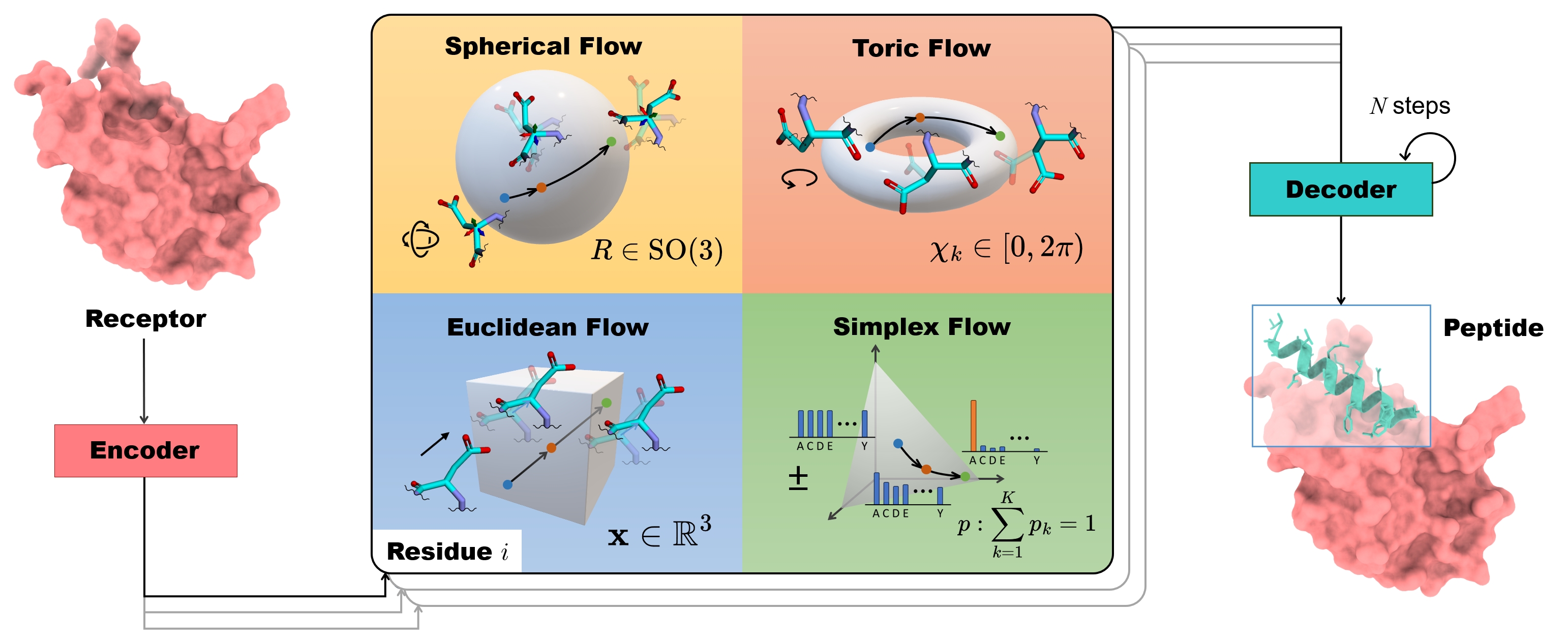
Figure 2: Illustration of PepFlow Architecture. The encoder encodes the receptor as the context for peptide generation. Flows for four different modalities are then constructed: spherical for the orientation $R$, Euclidean for the translation $\mathbf{x}$, toric for the torsion angles $\chi_{k}$, and categorical for the type distribution $p$. The multi-modal flow matching decoder finally recovers the full-atom peptide structure and sequence iteratively using the Euler method.

The conditional flow matching framework (Lipman et al., 2022) provides a simple yet powerful way to learn a probability flow $\psi$ that pushes the source distribution $p_{0}$ to the target distribution $p_{1}$ of the data points $\mathbf{x}\in\mathbb{R}^{d}$. The time-dependent flow $\psi_{t}:[0,1]\times\mathbb{R}^{d}\rightarrow\mathbb{R}^{d}$ and the associated vector field $u_{t}:[0,1]\times\mathbb{R}^{d}\rightarrow\mathbb{R}^{d}$ can be defined via the Ordinary Differential Equation (ODE) $\frac{d}{dt}\mathbf{x}_{t}=u_{t}(\mathbf{x}_{t})$ where $\mathbf{x}_{t}=\psi_{t}(\mathbf{x_{0}})$. A time-dependent network $v_{\theta}(\mathbf{x}_{t},t)$ can be used to directly regress the defined vector field, known as the Flow Matching objective (FM). However, the FM objective is intractable in practice, as we have no access to the closed-form vector field $u_{t}$. Nonetheless, when conditioning the time-dependent vector field and probability flow on the specific sample $\mathbf{x}_{1}\sim p_{1}(\mathbf{x}_{1})$ and the prior sample $\mathbf{x}_{0}\sim p_{0}(\mathbf{x}_{0})$, we can model $\mathbf{x}_{t}=\psi_{t}(\mathbf{x}_{0}|\mathbf{x}_{1})$ and $u_{t}(\mathbf{x}_{t}|\mathbf{x}_{0},\mathbf{x}_{1})=\frac{d}{dt}\mathbf{x}_{t}$ with the tractable Conditional Flow Matching (CFM) objective:

$$\mathcal{L}(\theta)=\mathbb{E}_{t,p_{1}(\mathbf{x}_{1}),p_{0}(\mathbf{x}_{0})}\|v_{\theta}(\mathbf{x}_{t},t)-u_{t}(\mathbf{x}_{t}|\mathbf{x}_{1},\mathbf{x}_{0})\|^{2}$$ (1)

where $t\sim\mathcal{U}(0,1)$. It has been proved that the FM and CFM objectives have identical gradients with respect to the parameters $\theta$, and we can integrate the learned vector field through time for sampling. Chen & Lipman (2023) further extended CFM to general geometries.

We employ the conditional flow matching framework to learn the conditional distribution of an $n$-residue peptide based on its $m$-residue target protein $p(C^{\text{pep}}|C^{\text{rec}})$. We empirically decompose the joint probability into the product of probabilities of four basic elements that can describe the sequence and structure:

$$p(C^{\text{pep}}|C^{\text{rec}}) \propto p(\{a^{j}\}_{j=1}^{n}|C^{\text{rec}})p(\{R^{j}\}_{j=1}^{n}|C^{\text{rec}})$$ (2)

$$\quad\cdot p(\{\mathbf{x}^{j}\}_{j=1}^{n}|C^{\text{rec}})p(\{\chi^{j}\}_{j=1}^{n}|C^{\text{rec}})$$

We elaborate on the construction of different probability flows on the residue’s position $p(x^{j}|C^{\text{rec}})$, orientation $p(R^{j}|C^{\text{rec}})$, torsion angles $p(\mathbf{\chi}^{j}|C^{\text{rec}})$, and type $p(a^{j}|C^{\text{rec}})$ as follows. For simplicity, we initially focus on the single $j$-th residue in the peptide.

Euclidean CFM for Position

We first adopt Euclidean CFM for the position vector $\mathbf{x}^{j}\in\mathbb{R}^{3}$. As a common practice, we choose the isotropic Gaussian $\mathcal{N}(0,I_{3})$ as the prior, and our target distribution is $p(\mathbf{x}^{j}|C^{\text{rec}})$. The conditional flow is defined as linear interpolation connecting sampled noise $\mathbf{x}_{0}^{j}\sim\mathcal{N}(0,I_{3})$ and the data point $\mathbf{x}_{1}^{j}\sim p(\mathbf{x}^{j}|C^{\text{rec}})$. The linear interpolation favors a straight trajectory, and such a property contributes to the efficiency of training and sampling, as it is the shortest path between two points in Euclidean space (Liu et al., 2022). The conditional vector field $u_{t}^{\text{pos}}$ is derived by taking the time derivative of the linear flow $\psi_{t}^{\text{pos}}$:

$$\psi_{t}^{\text{pos}}(\mathbf{x}_{0}^{j}|\mathbf{x}_{1}^{j}) =t\mathbf{x}_{1}^{j}+(1-t)\mathbf{x}_{0}^{j}$$ (3)

$$u_{t}^{\text{pos}}(\mathbf{x}_{t}^{j}|\mathbf{x}_{1}^{j},\mathbf{x}_{0}^{j}) =\mathbf{x}_{1}^{j}-\mathbf{x}_{0}^{j}=\frac{\mathbf{x}_{1}^{j}-\mathbf{x}_{t}^{j}}{1-t}$$ (4)

We use a time-dependent translation-invariant neural network $v^{\text{pos}}$ to predict the conditional vector field based on the current interpolant $\mathbf{x}_{t}$ and the timestep $t$. The CFM objective of the $j$ th residue is formulated as:

$$\mathcal{L}^{\text{pos}}_{j}=\mathbb{E}_{t,p(\mathbf{x}_{1}^{j}),p(\mathbf{x}_{0}^{j})}\left\|v^{\text{pos}}(\mathbf{x}_{t}^{j},t,C^{\text{rec}})-(\mathbf{x}_{1}^{j}-\mathbf{x}_{0}^{j})\right\|_{2}^{2}$$ (5)

During generation, we first sample from the prior $\mathbf{x}^{j}_{0}\sim\mathcal{N}(0,I_{3})$ and solve the probability flow with the learned predictor $v^{\text{pos}}$ using the $N$-step forward Euler method to get the position of residue $j$ with $t=\{0,...,\frac{N-1}{N}\}$:

$$\mathbf{x}_{t+\frac{1}{N}}^{j}=\mathbf{x}_{t}^{j}+\frac{1}{N}v^{\text{pos}}(\mathbf{x}_{t}^{j},t,C^{\text{rec}})$$ (6)

Spherical CFM for Orientation

The orientation of the residue $j$ can be represented as a rotation matrix $R^{j}\in\mathrm{SO}(3)$ concerning the global frame. The 3D rotation group $\mathrm{SO}(3)$ is a smooth Riemannian manifold and its tangent $\mathfrak{so}(3)$ is a Lie group containing skew-symmetric matrices. An element in $\mathfrak{so}(3)$ can also be interpreted as an infinitesimal rotation around a certain axis and characterized as a rotation vector in $\mathbb{R}^{3}$ (Blanco-Claraco, 2021). We choose the uniform distribution over $\mathrm{SO}(3)$ as our prior distribution. Just as flow matching in Euclidean space uses the shortest distance between two points, we can envision establishing flows by following the corresponding geodesics in the context of $\mathrm{SO}(3)$ (Lee, 2018). Geodesics on $\mathrm{SO}(3)$ represent the paths of the minimum rotational distance between two orientations and provide a natural way to interpolate and evolve orientations in a manner that respects the underlying geometry of the rotation manifold (Bose et al., 2023; Yim et al., 2023a). The conditional flow $\psi^{\text{ori}}$ and vector field $u_{t}^{\text{ori}}$ are established by the geodesic interpolation between $R^{j}_{0}\sim U(\mathrm{SO}(3))$ and $R_{1}^{j}\in p(R^{j}|C^{\text{rec}})$ with the geodesic distance decreasing linearly by time:

$$\psi^{\text{ori}}_{t}(R^{j}_{0}|R^{j}_{1}) =\mathtt{exp}_{R_{0}^{j}}(t\mathtt{log}_{R_{0}^{j}}(R_{1}^{j}))$$ (7)

$$u_{t}^{\text{ori}}(R_{t}^{j}|R_{0}^{j},R_{1}^{j}) =\frac{\mathtt{log}_{R_{t}^{j}}R_{1}^{j}}{1-t}$$ (8)

where $\mathtt{exp}$ and $\mathtt{log}$ are the exponential and logarithm maps on $\mathrm{SO}(3)$ that can be computed efficiently using Rodrigues’ formula (see Appendix A.1). A rotation-equivariant neural network $v^{\text{ori}}$ is applied to predict the vector field, represented as rotation vectors. The CFM objective on $\mathrm{SO}(3)$ is formulated as:

$$\mathcal{L}_{\text{ori}}^{j}=\mathbb{E}_{t,p(R_{1}^{j}),p(R_{0}^{j})}\left\|v^{\text{ori}}(R_{t}^{j},t,C^{\text{rec}})-\frac{\mathtt{log}_{R_{t}^{j}}R_{1}^{j}}{1-t}\right\|_{\mathrm{SO}(3)}^{2}$$ (9)

where the vector field lies on the tangent space $\mathfrak{so}(3)$ of $\mathrm{SO(3)}$ and the norm is induced by the canonical metric on $\mathrm{SO(3)}$. During inference, we initiate the process from $R^{j}_{0}\sim U(\mathrm{SO}(3))$ and proceed by taking small steps along the geodesic path in $\mathrm{SO}(3)$ over the timestep $t$:

$$R_{t+\frac{1}{N}}^{j}=\mathtt{exp}_{R_{t}^{j}}\left(\frac{1}{N}v^{\text{ori}}(R_{t}^{j},t,C^{\text{rec}})\right)$$ (10)

Toric CFM for Angles

An angle taking values in $[0,2\pi)$ can be represented as a point on the unit circle $\mathbb{S}^{1}$, and the torsion vector $\chi^{j}$ consisting $5$ angles lies on the $5$-dimensional flat torus $\mathbb{T}^{d}=(\mathbb{S}^{1})^{5}$ as the Cartesian product of $5$ one-dimensional unit circles. The flat torus $\mathbb{T}^{5}$ can also be viewed as the quotient space $\mathbb{R}^{5}/(2\pi\mathbb{Z})^{5}$ that inherits its Riemannian metric from Euclidean space. Therefore, the exponential and logarithm maps are similar to those in Euclidean space except for the equivalence relation about the periodicity of $2\pi$. We choose the uniform distribution on $[0,2\pi]^{5}$ as the prior distribution, and the conditional flow between sampled points $\chi^{j}_{0}\sim U([0,2\pi]^{5})$ and $\chi^{j}_{1}\sim p(\chi^{j}|C^{\text{rec}})$ is constructed along the geodesic:

$$\text{wrap}(u) =(u+\pi)\%(2\pi)-\pi$$ (11)

$$\psi_{t}^{\text{ang}}(\chi_{0}^{j}|\chi_{1}^{j}) =(\chi_{0}^{j}+t(\chi_{1}^{j}-\chi_{0}^{j}))\%2\pi$$ (12)

$$u_{t}^{\text{ang}}(\chi_{t}^{j}|\chi_{0}^{j},\chi_{1}^{j}) =\text{wrap}\left(\frac{\chi_{1}^{j}-\chi_{t}^{j}}{1-t}\right)$$ (13)

A neural network $v^{\text{ang}}$ is applied to predict the vector field that lies on the tangent space of $\mathbb{T}^{5}$, leading to the CFM objective on torus as:

$$\mathcal{L}_{\text{ang}}^{j}=\mathbb{E}_{t,p(\mathbf{\chi}_{1}^{j}),p(\mathbf{\chi}_{0}^{j})}\left\|\text{wrap}\left(v^{\text{ang}}(\mathbf{\chi}_{t}^{j},t,C^{\text{rec}})-\frac{\chi_{1}^{j}-\chi_{0}^{j}}{1-t}\right)\right\|^{2}$$ (14)

Instead of using the standard distance of the Euclidean space, we use the flat metric on $\mathbb{T}^{d}$ for comparing the predicted and ground truth vector field, which enhances the network’s awareness of angular periodicity on the toric geometry. During inference, we take Euler steps from prior sample points $\chi^{j}\sim U([0,2\pi]^{5})$ along the geodesic path in $\mathbb{T}^{5}$:

$$\chi^{j}_{t+\frac{1}{N}}=\left(\chi^{j}_{t}+\frac{1}{N}v^{\text{ang}}(\mathbf{\chi}_{t}^{j},t,C^{\text{rec}})\right)\%2\pi$$ (15)

Simplex CFM for Type

The above flow-matching methods apply to values in continuous spaces. The residue type $a^{j}\in\{1...20\}$, however, admits a discrete categorical value. To map the discrete residue type $a^{j}$ to a continuous space, we adopt a soft one-hot encoding operation $\mathtt{logit}(a^{j})=\mathbf{s}^{j}\in\mathbb{R}^{20}$ with a constant value $K>0$, and the $i$-th value in $\mathbf{s}^{j}$ is

$$\mathbf{s}^{j}[i]=\begin{cases}K,&i=a^{j}\\ -K,&\text{otherwise}\end{cases}$$ (16)

$\mathbf{s}^{j}$ can be understood as the logits of the probabilities (Han et al., 2023), and $\mathtt{softmax}(\mathbf{s}^{j})$ becomes a normalized probability distribution with the $j$-th term close to $1$ and other terms close to $0$. This representation promotes the underlying categorical distribution with a probability mass centered on the correct residue type $a^{j}$. In other word, $\mathtt{softmax}(\mathbf{s}^{j})$ is a point on the $20$-category probability simplex $\Delta^{19}$. The $d$-categorical probability simplex $\Delta^{d-1}:=\{\mathbf{x}\in\mathbb{R}^{d}:0\leq\mathbf{x}[i]\leq 1,\sum_{i=1}^{d}\mathbf{x}[i]=1\}$ is a smooth manifold in $\mathbb{R}^{d}$ (Wang & Carreira-Perpinán, 2013; Richemond et al., 2022; Floto et al., 2023), where each point in $\Delta^{d-1}$ represents a categorical distribution over the $d$ classes. Though we can directly perform flow matching on $\Delta^{d-1}$ (Li, 2018), we choose to construct conditional flow on the logit space in $\mathbb{R}^{d}$. We choose our prior distribution of logit as $\mathcal{N}(0,K^{2}I)$ such that the prior distribution on simplex becomes the logistic-normal distribution by construct (Atchison & Shen, 1980). The conditional flow $\psi_{t}^{\text{type}}$ and vector field on the logit space is defined as:

$$\psi_{t}^{\text{type}}(\mathbf{s}_{0}^{j}|\mathbf{s}_{1}^{j}) =t\mathbf{s}_{1}^{j}+(1-t)\mathbf{s}_{0}^{j}$$ (17)

$$u_{t}^{\text{type}}(\mathbf{s}_{t}^{j}|\mathbf{s}_{1}^{j},\mathbf{s}_{0}^{j}) =\mathbf{s}_{1}^{j}-\mathbf{s}_{0}^{j}=\frac{\mathbf{s}_{1}^{j}-\mathbf{s}_{t}^{j}}{1-t}$$ (18)

The linear interpolations between $\mathbf{s}^{j}_{1}$ and $\mathbf{s}^{j}_{0}$ induce a geometric mean of the prior logit-normal distribution and target distribution $p(a_{j}|C^{\text{rec}})$. This induces a time-dependent interpolant between points on the probability simplex, capturing the evolving relationship between the prior and target distributions. Similarly, a neural network $v^{\text{type}}$ is applied to predict the vector field on the logit space, and the CFM objective is:

$$\mathcal{L}^{\text{type}}_{j}=\mathbb{E}_{t,p(\mathbf{s}_{1}^{j}),p(\mathbf{s}_{0}^{j})}\left\|v^{\text{type}}(\mathbf{s}_{t}^{j},t,C^{\text{rec}})-(\mathbf{s}_{1}^{j}-\mathbf{s}_{0}^{j})\right\|_{2}^{2}$$ (19)

During inference, we perform Euler steps to solve the probability flow on the logit space, residue types can be sampled from the corresponding probability vector on the simplex:

$$\mathbf{s}_{t+\frac{1}{N}}^{j} =s_{t}^{j}+\frac{1}{N}v^{\text{type}}(\mathbf{s}_{t}^{j},t,C^{\text{rec}})$$ (20)

$$a^{j}_{t+1/N} \sim\mathtt{softmax}(\mathbf{s}_{t+\frac{1}{N}}^{j})$$ (21)

To improve generation consistency between the logit and simplex space, we additionally map the predicted discrete residue back to the logit space during each iteration as $\mathbf{s}_{t+1/N}^{j}=\mathtt{logit}(a^{j}_{t+\frac{1}{N}})$.

Combining all modalities, we obtain the final multi-modal conditional flow matching objective for residue $j$ as the weighted sum of different conditional flow matching objectives:

$$\mathcal{L}^{j}_{\text{cfm}}=\mathbb{E}_{t}(\lambda^{\text{pos}}\mathcal{L}^{\text{pos}}_{j}+\lambda^{\text{ori}}\mathcal{L}^{\text{ori}}_{j}+\lambda^{\text{ang}}\mathcal{L}^{\text{ang}}_{j}+\lambda^{\text{type}}\mathcal{L}^{\text{type}}_{j})$$ (22)

After discussing the multi-modal flow for modeling the factorized distribution of position, orientation, residue type, and side-chain torsion angles for a single residue $j$, we further extend our method for modeling the joint distribution $p(C^{\text{pep}}|C^{\text{rec}})$ in the following subsection.

3.3 PepFlow Architecture

Network Parametrization

As the joint distribution of the peptide is conditioned on its target protein receptor, we employ a geometric equivariant encoder to capture the context information of the target protein. Conversely, the above flow matching model can be viewed as a decoder for regressing the vector fields of the generated peptide, as depicted in Figure 2. In the model pipeline, the encoder $\mathrm{Enc}$ takes the sequence and structure of the target protein $C^{\text{rec}}$, producing the hidden residue representations $\mathbf{h}$ and the residue-pair embedding $\mathbf{z}$. Subsequently, we sample a specific timestep $t\sim U(0,1)$ to construct the multi-modal flows where time-dependent vector fields are learned simultaneously for each modality of the peptide $C^{\text{pep}}$. The time-dependent decoder network $\mathrm{Dec}$, mainly based on the Invariant Point Attention scheme (Jumper et al., 2021), takes the timestep $t$, the interpolant state of the peptide $C^{\text{pep}}_{t}=\{(\mathbf{s}^{j}_{t},R^{j}_{t},\mathbf{x}^{j}_{t},\chi^{j}_{t})\}_{j=1}^{n}$, and the residue and pair embeddings as input. Rather than directly regressing the vector fields, the decoder first recovers the original peptide $\overline{C}^{\text{pep}}_{1}=\{(\overline{\mathbf{s}}^{j}_{1},\overline{R}^{j}_{1},\overline{\mathbf{x}}^{j}_{1},\overline{\chi}^{j}_{1})\}_{j=1}^{n}$ which allows for better training efficiency and the use of auxiliary loss. In this way, the CFM objectives for different modalities are reparametrized as the distance between the vector fields derived from ground truth elements and those derived from predicted elements (see Appendix A.2). The overall training objective is the sum of reparameterized CFM objectives, considering the expectation over each timestep and each residue in the peptide.

$$\mathcal{L}=\mathbb{E}_{t}\left[\frac{1}{n}\sum_{j}(\mathcal{L}^{j}_{\text{cfm}}+\lambda^{\text{aux}}(\mathcal{L}^{j}_{\text{bb}}+\mathcal{L}^{j}_{\text{tor}}))\right]$$ (23)

Here we also use the backbone position loss $\mathcal{L}_{\text{bb}}$ and the torsion angle loss $\mathcal{L}_{\text{tor}}$ as auxiliary structure losses to improve the generation quality, incorporating information from different modalities (see Appendix A.5). The training process is outlined in Algorithm 1.

Algorithm 1 Training Multi-Modal PepFlow

1:  while not converged do

2:     Sample protein-peptide pair $C^{\text{rec}},C^{\text{pep}}$ from dataset

3:     Encode target $\mathbf{h,z}=\mathrm{Enc}(C^{\text{rec}})$

4:     Sample prior state $C^{\text{pep}}_{0}=\{(a^{j}_{0},R^{j}_{0},\textbf{x}^{j}_{0},\chi^{j}_{0})\}_{j=1}^{n}$

5:     Sample $t\sim U(0,1)$

6:     Decode predicted peptide $\overline{C}^{\text{pep}}=\mathrm{Dec}(C^{\text{pep}}_{t},t,\mathbf{h,z})$

7:     Calculate the vector fields and the loss according to Eq.(23)

8:     Update the parameters of $\mathrm{Enc}$ and $\mathrm{Dec}$

9:  end while

Sampling Process

The sampling algorithm is outlined in Algorithm 2. During sampling, the target protein is encoded only once and is fed into each step of decoding. Initially, a prior state of the peptide is sampled. Subsequently, for each timestep of the sampling, the decoder predicts the recovered peptide state, and vector fields are calculated for each modality of the current state. The current state of the peptide is then updated using the Euler method following the derived vector fields, and the updated peptide is considered as the input of the decoder in the subsequent iteration. In the final step, we reconstruct the full-atom peptide using local coordinate transformations of the backbone and side-chain rigid groups (Jumper et al., 2021).

Noticeably, for a specific residue, the generation of a particular modality is not only dependent on the update of that modality but also influenced by the states of other modalities and other residues within the peptide. This interdependence highlights the intricate relationship between different modalities and residues, illustrating the complex nature of the joint distribution captured by our designed decoder network.

Algorithm 2 Sampling with Multi-Modal PepFlow

1:  Encode target $\mathbf{h,z}=\mathrm{Enc}(C^{\text{rec}})$

2:  Sample prior state $C^{\text{pep}}_{0}=\{(a^{j}_{0},R^{j}_{0},\textbf{x}^{j}_{0},\chi^{j}_{0})\}_{j=1}^{n}$

3:  for $t\leftarrow 1$ to $N$ do

4:     Decode predicted peptide $\overline{C}^{\text{pep}}_{\frac{t}{N}}=\mathrm{Dec}(C^{\text{pep}}_{\frac{t-1}{N}},t,\mathbf{h,z})$

5:     Calculate vector fields and update the peptide $C^{\text{pep}}_{\frac{t}{N}}=\mathrm{EulerStep}(\overline{C}^{\text{pep}}_{\frac{t}{N}},C^{\text{pep}}_{\frac{t-1}{N}},\frac{1}{N})$

6:  end for

7:  return $\overline{C}^{\text{pep}}_{1}$

Furthermore, beyond the joint design of sequences and structures, we can construct partial states tailored for peptide design tasks that specifically emphasize the generation of a particular modality while keeping other modalities fixed. In the context of side-chain packing, we maintain the ground truth sequence and the backbone structure (i.e., types, positions, and orientations), and exclusively sample the torsion angles. Conversely, in fix-backbone sequence design, our focus lies in sampling sequences while holding constant the backbone positions and orientations.

4 Experiment

Table 1: Evaluation of methods in the sequence-structure co-design task.

	Geometry				Energy		Design
	AAR $\%\uparrow$	RMSD $\AA\downarrow$	SSR $\%\uparrow$	BSR $\%\uparrow$	Stability $\%\uparrow$	Affinity $\%\uparrow$	Designability $\%\uparrow$	Diversity $\uparrow$
RFdiffusion	40.14	4.17	63.86	26.71	26.82	16.53	78.52	0.38
ProteinGenerator	45.82	4.35	29.15	24.62	23.48	13.47	71.82	0.54
Diffusion	47.04	3.28	74.89	49.83	15.34	17.13	48.54	0.57
PepFlow w/Bb	50.46	2.30	82.17	82.17	14.04	18.10	50.03	0.64
PepFlow w/Bb+Seq	53.25	2.21	85.22	85.19	19.20	19.39	56.04	0.50
PepFlow w/Bb+Seq+Ang	51.25	2.07	83.46	86.89	18.15	21.37	65.22	0.42

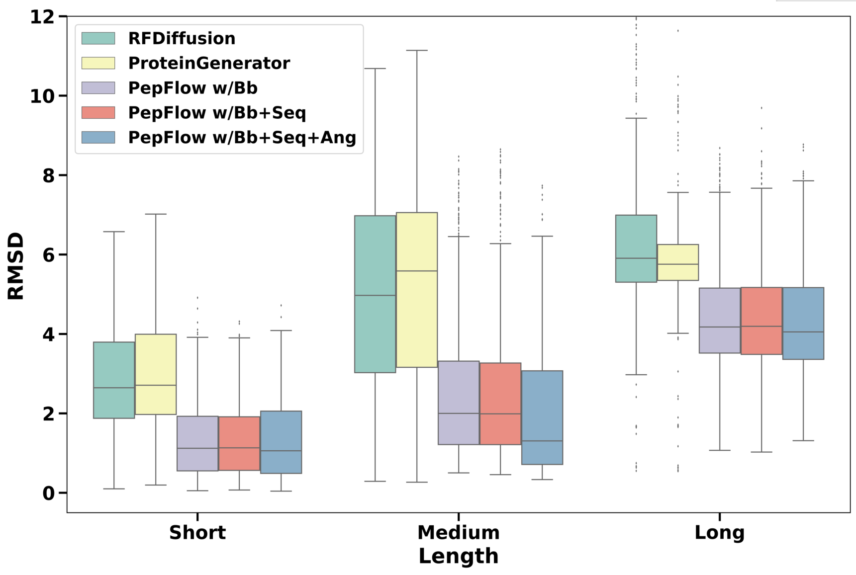
Figure 3: Left: RMSD of designed peptides of different lengths. (Short: 3-9, Medium: 10-14, Long: 15-25) Middle: Ramachandran plot of PepFlow generated and native peptides. Right: Binding energy distributions of generated and native peptides. (lower is better)

Figure 4: Three examples of the generated peptides. Top: native peptides; Bottom: generated peptides. PDB: 3MXY, 6OX4, 5DJY.

In this section, we conduct a comprehensive evaluation of PepFlow across three tasks: (1) Sequence-Structure Co-design, (2) Fix-Backbone Sequence Design, and (3) Side-Chain Packing. We introduce a new benchmark dataset derived from PepBDB (Wen et al., 2019) and Q-BioLip (Wei et al., 2024). After removing duplicate entries and applying empirical criteria (e.g. resolution $\textless 4\AA$, peptide length between $3-25$), we cluster these complexes according to $40\%$ peptide sequence identity using mmseqs2 (Steinegger & Söding, 2017). This results in $8,365$ non-orphan complexes distributed across $292$ clusters. To construct the test set, We randomly select $10$ clusters containing $158$ complexes, while the remaining complexes are used for training and validation.

We implement and compare the performance of three variants of our model. PepFlow w/Bb only samples backbones; PepFlow w/Bb+Seq is used for modeling backbones and sequences jointly; and PepFlow w/Bb+Seq+Ang finally model the full-atom distributions of peptides. Experimental details and additional results are provided in Appendix B.

4.1 Sequence-Structure Co-design

This task requires the generation of both the sequence and bound-state structure of the peptide based on its target protein. Models take the full-atom structure of the target protein as input and generate bound-state peptides. We generate $64$ peptides for each target protein for every evaluated model.

Baselines We use two state-of-the-art protein design models as baselines. RFDiffusion (Watson et al., 2022) generates protein backbones, and sequences are later predicted by ProteinMPNN (Dauparas et al., 2022). ProteinGenerator (Lisanza et al., 2023) improves RFDiffusion by jointly sampling backbones and corresponding sequences. These two methods do not consider side-chain conformations.

Metrics We assess the generated peptides from three perspectives. (1) Geometry. The generated peptides should exhibit sequences and structures similar to those of the native ones. The amino acid recovery rate (AAR) measures the sequence identity between the generated and the ground truth. The root-mean-square deviation (RMSD) aligns the complex by peptide structures and calculates the C_α RMSD. The secondary-structure similarity ratio (SSR) calculates the proportion of shared secondary structures. The binding site ratio (BSR) is the overlapping ratio between the binding site of the generated peptide and the native binding site on the target protein. (2) Energy. We aim to design high-affinity peptide binders that stabilize the protein-peptide complexes. Affinity is the percentage of the designed peptides with higher binding affinities (lower binding energies) than the native peptide, and Stability calculates the percentage of complex structures that are at more stable (lower total energy) states than the native ones. The energy terms are calculated by Rosetta (Alford et al., 2017). (3) Design. Designablity measures the consistency between generated sequences and structures by counting the fractions of sequences that can fold into similar structures as the corresponding generated structure. We utilize ESMFold (Lin et al., 2023) to refold sequences and use C_α RMSD <2Åas designable criteria. Diversity is the average of one minus the pair-wise TM-Score (Zhang & Skolnick, 2005) among the generated peptides, reflecting structural dissimilarities.

Results As indicated in Table 1, PepFlow is capable of generating peptides that closely resemble native ones with improved binding affinities. The distributions of generated backbone torsion angles also closely align with the native peptide distributions (see Figure 3). Since the generation of structure and sequence is decoupled, RFDiffusion exhibits the lowest recovery, whereas PepFlow achieves lower RMSD and higher AAR by incorporating the sequence modality. Moreover, the explicit modeling of side-chain conformations effectively captures the fine-grained structures in protein-peptide interactions, enhancing the ability of generated peptides to accurately bind to designated binding sites. Consequently, the proportion of peptides with higher affinity is also increased. We also observe that baselines outperformed our models in terms of Stability and Designability, probably because they are trained on the entire PDB structures and are biased toward structures with more stable motifs. Additionally, we note that modeling more modalities leads to a slightly lower diversity of refolded structures. Nevertheless, our results demonstrate that incorporating sequence and side-chain conformation, beyond modeling the backbone, significantly improved the model’s performance, underscoring the importance of full-atom modeling.

Visualizations We further present three examples of generated full-atom peptides generated by full-atom PepFlow in Figure 4. We observe that PepFlow consistently produces peptides with topologically resembling geometries, regardless of the native length. Remarkably, the generated peptides exhibit similar side-chain compositions and conformations, facilitating effective interaction with the target protein at the correct binding site.

4.2 Fix-backbone Sequence Design

This task involves designing peptide sequences based on the structure of the complex without side-chains. We generate $64$ sequences for each peptide using each model. For our models, we apply the partial sampling scheme to recover the sequence.

Table 2: Evaluations of methods in the fix-backbone sequence design task.

	AAR $\%\uparrow$	Worst $\%\uparrow$	Likeness $\downarrow$	Diversity $\uparrow$	Designbility $\%\uparrow$
ProteinMPNN	53.28	45.99	-8.42	15.33	60.55
ESM-IF	43.51	36.18	-8.39	13.76	53.76
PepFlow w/Bb+Seq	56.40	46.59	-8.26	23.38	59.72
PepFlow w/Bb+Seq+Ang	54.32	44.48	-8.58	20.65	65.48

Baselines We use two inverse folding models which can design peptide sequences conditioned on the rest of the complex as our baselines: Protein-MPNN (Dauparas et al., 2022), a GNN-base model, and ESM-IF (Hsu et al., 2022), based on GVP-Transformer (Jing et al., 2020).

Metrics In addition to AAR used in co-design task, we calculate Worst as the lowest recovery rate. Likeness is the negative log-likelihood score of the sequence from ProtGPT2 (Ferruz et al., 2022), indicating how closely the generated sequence aligns with the native protein distribution. Diversity represents the average pairwise Hamming Distance between generated sequences.

Results As presented in Table 2, our models achieve higher recovery rates and better diversities, showcasing the effectiveness of our proposed simplex flow matching. We also observe a slight decrease in the recovery rate with the inclusion of angle modeling. This might be attributed to the fact that some amino acids share similar side-chain compositions and physicochemical properties (e.g. Ser and Thr, Arg and Lys), leading the model to generate a physicochemically feasible but different residue. Generating both the sequences and side-chain angles leads to higher likeness and lower diversity.

4.3 Side-chain Packing

This task predicts the side-chain angles of the peptide. We generate $64$ side-chain conformations for each peptide by each model and apply the partial sampling scheme of our model to recover side-chain angles.

Table 3: Evaluation of methods in the side-chain packing task.

	MSE ${}^{\circ}\downarrow$
	$\chi_{1}$	$\chi_{2}$	$\chi_{3}$	$\chi_{4}$	Correct $\%\uparrow$
Rosseta	38.31	43.23	53.61	71.67	57.03
SCWRL4	30.06	40.40	49.71	53.79	60.54
DLPacker	22.44	35.65	58.53	61.70	60.91
AttnPacker	19.04	28.49	40.16	60.04	61.46
DiffPack	17.92	26.08	36.20	67.82	62.58
PepFlow w/Bb+Seq+Ang	17.38	24.71	33.63	58.49	62.79

Baselines Two energy-based methods: RossettaPacker (Leman et al., 2020), SCWRL4 (Krivov et al., 2009), and learning-based models: DLPacker (Misiura et al., 2022), AttnPacker (McPartlon & Xu, 2022), DiffPack (Zhang et al., 2023b).

Metrics We use the Mean Absolute Error (MAE) of predicted four torsion angles. Due to the flexibility of side-chains, We also include the proportion of the Correct predictions that deviate within $20^{\circ}$ around the ground truth.

Results As shown in Table 3, our partially sampling PepFlow outperforms all other baselines across all four side-chain angles. Notably, $\chi_{1}$ and $\chi_{2}$ angles are easier to predict than $\chi_{3}$ and $\chi_{4}$. Our method also achieves the best correct rates, as our proposed toric flow can precisely capture the reasonable distribution of the side-chain angles and the plausible side-chain dynamics during the interaction between peptides and target proteins.

5 Conclusion

In this study, we introduced PepFlow, a novel flow-based generative model tailored for target-specific full-atom peptide design. PepFlow characterizes each modality of peptide residues into the corresponding manifold and constructs analytical flows and vector fields for each modality. Through multi-modal flow matching objectives, PepFlow excels in generating full-atom peptides, capturing the intrinsic geometric characteristics across different modalities. In our newly designed comprehensive benchmarks, PepFlow has demonstrated promising performance by modeling full-atom joint distributions and exhibits potential applications in protein design beyond peptides, such as antibody and enzyme design. Nevertheless, PepFlow faces limitations in diversity during generation, stemming from the deterministic nature of ODE-based flow. Furthermore, its current incapability for property-guided generation, a common requirement in protein optimization, represents an area for improvement. Despite these considerations, PepFlow stands out as a potent and versatile tool for computational peptide design and analysis.

Impact Statement

PepFlow can contribute to the advancement of computational biology, particularly in the field of protein design, offering a valuable tool for designing therapeutic peptides with potential benefits for human health. While our primary focus is on positive applications, such as drug development and disease treatment, we recognize the importance of considering potential risks associated with any powerful technology. There is a possibility that our algorithm could be misused for designing harmful substances, posing ethical concerns. However, we emphasize the responsible and ethical use of our tool, urging the scientific community and practitioners to employ it judiciously for constructive purposes. Our commitment to ethical practices aims to ensure the positive impact of PepFlow on society.

Code and data are available at https://github.com/Ced3-han/PepFlowww.

Appendix A PepFlow Implementations

A.1 Manifold Explanations

In this subsection, we further introduce some basic concepts of Riemannian manifolds as well as some important properties of the manifolds used by PepFlow. A Riemannian manifold $\langle\mathcal{M},g\rangle$ is a real, smooth manifold $\mathcal{M}$ equipped with a positive-definite inner product $g$ on the tangent space $T_{p}\mathcal{M}$ at each point $p$. Let $T\mathcal{M}=\bigcup_{p\in\mathcal{M}}\{p\}\times T_{p}\mathcal{M}$ be the tangent bundle of the manifold, a time-dependent smooth vector field on $\mathcal{M}$ is a mapping $u_{t}:[0,1]\times\mathcal{M}\to T\mathcal{M}$ where $u_{t}(p)\in T_{p}(\mathcal{M})$ for all $p\in\mathcal{M}$.

A geodesic is a locally distance-minimizing curve on the manifold. The existence and the uniqueness of the geodesic state that for any point $p\in\mathcal{M}$ and for any tangent vector $u\in T_{p}(\mathcal{M})$, there exists a unique geodesic $\gamma:[0,1]\to\mathcal{M}$ such that $\gamma(0)=p$ and $\gamma^{\prime}(0)=u$. The exponential map $\mathtt{exp}_{p}:\mathcal{M}\times T\mathcal{M}\to\mathcal{M}$ is uniquely defined to be $\mathtt{exp}_{p}(u)=\gamma(1)$. The logarithm map $\mathtt{log}:\mathcal{M}\times\mathcal{M}\to T\mathcal{M}$ is defined as the inverse mapping of the exponential map such that $\mathtt{exp}_{p}(\mathtt{log}_{p}(q))\equiv q,\forall p,q\in\mathcal{M}$. The exponential map and logarithm map are central in terms of interpolation along the geodesic. As we have mentioned in the main text, the time-dependent flow can be compactly written as

$$\psi_{t}(p|p_{0},p_{1})=\mathtt{exp}_{p_{0}}(t\mathtt{log}_{p_{0}}p_{1})$$ (24)

It can be verified that the above formula indeed follows the geodesic between $p_{0}$ and $p_{1}$ with linearly decreasing geodesic distances between the interpolated point $p_{t}$ and the target $p_{1}$. For general manifolds, closed-form formulae for the exponential and logarithm maps are generally not available. However, the manifolds encountered in this work have well-understood geometries which make it possible for efficient training and sampling using the exponential and logarithm maps.

Euclidean manifold

The tangent space of the Euclidean space $\mathbb{R}^{d}$ is also $\mathbb{R}^{d}$, and the canonical inner product for $n$-dimensional vectors can be equipped to form a Riemannian manifold. The exponential map and logarithm map on the Euclidean manifold can be explicitly written as

$$\mathtt{exp}_{\mathbf{x}}(\mathbf{y}) =\mathbf{x}+\mathbf{y}$$ (25)

$$\mathtt{log}_{\mathbf{x}}(\mathbf{u}) =\mathbf{u}-\mathbf{x}$$ (26)

Intuitively, the geodesic between two points in the Euclidean space is exactly the line segment joining the two points, and interpolation at timestep $t$ is given linearly by $\psi_{t}(\mathbf{x}|\mathbf{x}_{0},\mathbf{x}_{1})=(1-t)\mathbf{x}_{0}+t\mathbf{x}_{1}$. This coincides with the common flow-matching loss for image generation, as already demonstrated in (Chen & Lipman, 2023).

Rotation group $\mathrm{SO}(3)$

The 3D rotation group or the special orthogonal group $\mathrm{SO}(3)$ is a compact 3-dimensional Lie group whose differential is a skew-symmetric matrix in the tangent space $\mathfrak{so}(3)$. The canonical choice of the inner product on the tangent space is the half of the induced Frobenius inner product:

$$\langle A,B\rangle_{\mathrm{SO}(3)}=\frac{1}{2}\langle A,B\rangle_{F}=\frac{1}{2}\mathrm{tr}(A^{\top}B),\forall A,B\in\mathfrak{so}(3)$$ (27)

This equips $\mathrm{SO}(3)$ with a Riemannian structure. The $\mathrm{SO}(3)$ manifold has a constant Gaussian curvature everywhere and is diffeomorphic to a solid ball with antipolar points identified. The exponential map (from the identity rotation $I$) $\mathtt{exp}:\mathfrak{so}(3)\to\mathrm{SO}(3)$ can be realized as the standard matrix exponentiation:

$$\mathtt{exp}(A)=\exp(A)=\sum_{k=0}^{\infty}\frac{A^{k}}{k!},\forall A\in\mathfrak{so}(3)$$ (28)

Rodrigues’ rotation formula gives an equivalent but more compact form of the exponential map as

$$\mathtt{exp}(A)=I+\frac{\sin\theta}{\theta}A+\frac{1-\cos\theta}{\theta^{2}}A^{2},\forall A\in\mathfrak{so}(3)$$ (29)

where $\theta=\|A\|_{\mathrm{SO}(3)}=\frac{1}{2}\|A\|_{F}$ represents the rotation angle. Similarly, the logarithm map (from the identity rotation $I$) $\mathtt{log}:\mathrm{SO}(3)\to\mathfrak{so}(3)$ can be defined as the matrix logarithm as

$$\mathtt{log}(R)=\log R=\sum_{k=1}^{\infty}(-1)^{k+1}\frac{(R-I)^{k}}{k}$$ (30)

or more compactly via

$$\mathtt{log}(R)=\frac{\theta}{\sin\theta}A,\forall R\in\mathrm{SO}(3)$$ (31)

where $A=(R-R^{\top})/2\in\mathfrak{so}(3)$ and $\theta=\|A\|_{\mathrm{SO}(3)}$ represents the rotation angle. Utilizing the sphere geometry, the geodesic distance between two rotations can be determined as $d(R_{1},R_{2})=\|\mathtt{log}(R_{1}^{\top}R_{2})\|_{F}$, and the interpolation can be calculated as $\mathtt{exp}(tA)$.

Special Euclidean group $\mathrm{SE}(3)$

The special Euclidean group $\mathrm{SE}(3)$ comprises of all rigid transformations of rotation and translation. It can be understood as the semidirect product of $\mathrm{SO}(3)$ and a translation vector in $\mathbb{R}^{3}$

$$\mathrm{SE}(3)=\mathrm{SO}(3)\ltimes\mathbb{R}^{3}$$ (32)

In practice, the interpolated rotation $R_{t}$ and translation $\mathbf{x}_{t}$ at timestep $t$ are fed into a common encoder. Different predictor heads are then applied to the hidden representation to predict the rotation and translation vector field. In this way, each head can leverage the information from both the rotation and translation to learn the joint distribution over $\mathrm{SE}(3)$.

Toric manifold

A flat torus in $n$ dimensions is characterized by a metric inherited from its representation as the quotient, $\mathbb{R}^{n}/L$, where $L$ denotes a discrete subgroup of $\mathbb{R}^{n}$ that is isomorphic to $\mathbb{Z}^{n}$. The tangent space of the torus corresponds to the Euclidean Space $\mathbb{R}^{n}$. In our study of torsional flow matching, $L$ represents the cartesian product of $2\pi\mathbb{Z}$ (Jantzen, 2012).

Since the flat torus inherits its metric from the quotient manifold, the exponential and logarithm maps can be understood as corresponding to their Euclidean counterparts with modulo of $2\pi$. In Eq.33, the logarithm map is represented as an array of angles that indicate the direction of the geodesic.

$$\mathtt{exp}_{a}(u) =(a+u)\%(2\pi)$$ (33)

$$\mathtt{log}_{a}(b) =\mathrm{atan2}(\sin(b-a),\cos(b-a))$$ (34)

Then we can derive the simplified vector field on the toric manifold, by definition, the atan2 function returns an angle in $(-\pi,\pi]$, and we can rewrite the logarithm map, which is locally and linearly connecting the displacement vectors:

$$\text{wrap}(u) =(u+\pi)\%(2\pi)-\pi$$ (35)

$$\log_{a}(b) =\text{wrap}(b-a)$$ (36)

Then the interpolation can be written as a locally straight line in the embedded Euclidean space connecting the starting point and end point:

$$\psi_{t}=\exp_{\chi_{0}^{j}}(t\log_{\chi_{0}^{j}}\chi_{1}^{j})=(\chi_{0}^{j}+t\text{wrap}(\chi_{1}^{j}-\chi_{0}^{j}))\%(2\pi)$$ (37)

Taking the derivative concerning $t$, we obtain the vector field as:

$$u_{t}=\frac{\partial\psi_{t}}{\partial t}=\text{wrap}(\chi_{1}^{j}-\chi_{0}^{j})=\text{wrap}\left(\frac{\chi_{1}^{j}-\chi_{t}^{j}}{1-t}\right)$$ (38)

Simplex manifold

A $(d-1)$-simplex $\Delta^{d-1}$ can be used to represent the collect of all $d$-class categorical distributions such that $\Delta^{d-1}=\{\mathbf{p}\in\mathbb{R}^{d},\|\mathbf{p}\|_{1}=1,0\leq p_{k}\leq 1,1\leq k\leq d\}$. In this way, each point $\mathbf{p}\in\Delta^{d-1}$ is a $d$-class categorical distribution on which a flow can be defined. Different from the common Euclidean setting, a simplex manifold is a bounded manifold. If we construct a flow directly on the simplex, we may encounter the problems of Points moving outside the boundaries. Note that the vector field on the boundary points outside the simplex. Point moving away from the manifold. Though this can be prevented by projecting the predicted vector fields onto the tangent space $\{\mathbf{u}|\sum_{k=1}^{n}u_{k}=0\}$. Therefore, even though directly working on the simplex has the advantage of being simpler to implement, we chose to work on the logit space which is well-defined over $\mathbb{R}^{n}$ for unconstraint flow matching. There is, however, one disadvantage of the projective structure of the logit space. In other words, the mapping between the simplex and the logit space is not one-to-one, as an equivariant class of a categorical distribution can be identified with $\mathbf{s}_{1}\sim\mathbf{s}_{1}\Leftrightarrow\exists C\in\mathbb{R}\text{ s.t. }s_{1,k}=s_{2,k}+C,1\leq k\leq n$. We addressed this problem by essentially setting the logit of the last class to 0.

We follow (Han et al., 2023) to assume the logit-normal distribution of the categorical distribution of the amino acid types. In other words, we assume that the logits $s_{k}=\log(p_{k}/p_{d}),1\leq k\leq d-1$ follow some normal distribution in $\mathbb{R}^{d}$. Such a transform provides a diffeomorphism from the interior of the simplex $(\Delta^{d-1})^{\circ}$ to $\mathbb{R}^{d-1}$ in which the standard Euclidean flow matching can be applied. It can be demonstrated that such a transform assigns the last class $d$ with a logit of 0. As the boundary of the simplex is excluded in such a logit transformation, we instead use soft one-hot encoding by assigning the ground truth class with a const logit value of $2K>0$ and other logits with $0$ to be consistent with the last class $d$. Note that after applying the softmax function, a logit vector represents the same categorical distribution when adding a constant value to all of the logits. Therefore, such an assignment of the logit values coincides with our definition in Eq.(15). Similarly, if the last class $d$ is the ground truth class, other logits are set to $-2K$ such that the softmax probabilities remain the same. In this way, the categorical flow matching loss will be symmetric for all classes. The common Euclidean exponential and logarithm map and linear interpolation are applied on $\mathbb{R}^{d-1}$ for learning the vector field. The final amino acid types are sampled from the last categorical distribution. For all cases, we empirically set $K=5$.

A.2 Reparameterized CFM objectives

The Riemannian flow matching paper used the formulation of the object of the conditional vector field as

$$\mathcal{L}(\theta)=\mathbb{E}_{t,p_{1}(x_{1}),p_{0}(x_{0})}\|v_{\theta}(x_{t},t)-u_{t}(x_{t}|x_{1},x_{0})\|_{g}^{2}$$ (39)

where the time-dependent model $v_{\theta}$ directly learns the vector field at timestep $t$. Following the techniques used in various diffusion models, we can instead predict the target data at timestep $t=1$ and reparameterize the objective as

$$\mathcal{L}(\theta)=\mathbb{E}_{t,p_{1}(x_{1}),p_{0}(x_{0})}\|u_{t}(x_{t}|\hat{x}_{1},x_{0})-u_{t}(x_{t}|x_{1},x_{0})\|_{g}^{2}$$ (40)

where $\hat{x}_{1}=v_{\theta}(x_{t},t)$. In this formulation, the vector field between the reconstructed data $\hat{x}_{1}$ and the noise $x_{0}$ are calculated and compared to the ground truth vector field. Specifically, for flowing matching on Euclidean manifolds, we have $u_{t}(\mathbf{x}_{t}|\mathbf{x}_{1},\mathbf{x}_{0})=\mathbf{x}_{1}-\mathbf{x}_{0}$, and

$$\mathcal{L}_{\text{pos}}=\mathbb{E}_{t,p_{1}(\mathbf{x}_{1}),p_{0}(\mathbf{x}_{0})}\|(\hat{\mathbf{x}}_{1}-\mathbf{x}_{0})-(\mathbf{x}_{1}-\mathbf{x}_{0})\|_{2}^{2}=\mathbb{E}_{t,p_{1}(\mathbf{x}_{1}),p_{0}(\mathbf{x}_{0})}\|\hat{\mathbf{x}}_{1}-\mathbf{x}_{1}\|_{2}^{2}$$ (41)

which coincides with the mean squared error loss. Similarly, the reparameterized loss of the orientation, dihedral angles, and sequence can be formulated as

$$\mathcal{L}_{\text{ori}} =\mathbb{E}_{t,p_{1}(R_{1}),p_{0}(R_{0})}\left\|\left(\mathtt{log}_{\hat{R}_{t}}\hat{R}_{1}-\mathtt{log}_{R_{t}}R_{1}\right)/(1-t)\right\|_{\mathrm{SO}(3)}^{2}$$ (42)

$$\mathcal{L}_{\text{ang}} =\mathbb{E}_{t,p_{1}(\chi_{1}),p_{0}(\chi_{0})}\left\|(\hat{\chi}_{1}-\chi_{1})\%2\pi\right\|_{2}^{2}$$ (43)

$$\mathcal{L}_{\text{type}} =\mathbb{E}_{t,p_{1}(\mathbf{s}_{1}),p_{0}(\mathbf{s}_{0})}\left\|\hat{\mathbf{s}}_{1}-\mathbf{s}_{1}\right\|_{2}^{2}$$ (44)

Empirically, such parameterization makes the model more numerically stable while $t$ is close to 1 during sampling. Auxiliary losses based on the ground truth data are also feasible to calculate based on the reconstruction, as we will describe in detail in Appendix A.5. During training, we take the ground truth peptide state $C^{\text{pep}}$ and predicted peptide state $\overline{C}^{\text{pep}}$to calculate vector fields and CFM losses; during sampling, we take vector fields which start from the prior peptide state $C^{\text{pep}}_{\frac{t-1}{N}}$ to the current predicted peptide state $\overline{C}^{\text{pep}}_{\frac{t}{N}}$ for updating the prior state to the next state $C^{\text{pep}}_{\frac{t}{N}}$.

We would also like to mention that since different amino acids have varying numbers of side-chain angles, directly calculating torsion loss based on the real amino acid sequence might lead to potential data leakage. This situation could cause the sequence modality to rely on the number of torsions to predict amino acid types instead of learning the underlying biological connections. Therefore, during training, we pragmatically use the predicted amino acid sequence to guide the computation of torsion loss concerning side-chains. For instance, for the $j$-th amino acid, if its true type is LEU but it is predicted as ARG, we use the four side-chain angles of ARG to calculate the angle-related loss, rather than employing the two side-chain angles of LEU. This approach compels the model to treat the two extra side-chain angles from the real type as the default value of 0. In the generation phase, we directly reconstruct side-chain atomic coordinates based on the predicted amino acid type, using the corresponding number of the side-chain angles and the side-chain atomic composition.

A.3 Geometric Symmetries

We model the position $\mathbf{x}_{j}$ and orientation $R_{j}$ of each residue as a point in the Riemannian manifolds $\mathbb{R}^{3}$ and $\mathrm{SO}(3)$ such that the frame $T_{j}=(\mathbf{x}_{j},R_{j})$ lies on the Riemannian manifold $\mathrm{SE}(3)$. When extending to the whole peptide with $n$ residues, the set of $n$ frames should lie on a subspace of the Cartesian product of $n$ manifolds, $\mathrm{SE}(3)^{n}$ with a well-defined $\mathrm{SE}(3)$-invariant metric. To achieve that, we translate the entire protein-peptide complex by subtracting the mean positions of the $n$ residues in the peptide. This ensures that the $n$ positions of the peptide are in the zero center of mass subspace in Euclidean Space and renders the distribution of the generated peptide frames $\mathrm{SE}(3)$-invariant. The defined flows are also $\mathrm{SE}(3)$-invariant, and the vector fields for positions and orientations are $\mathrm{SE}(3)$-equivariant by the use of an equivariant IPA decoder (see Appendix A.4). For the modeling of torsion angles, side chain angles of some residues are $\pi$-rotation-symmetric, which means $\chi\in\mathbb{S}^{1}$ and the alternative $\chi+\pi\in\mathbb{S}^{1}$ will result in the same physical structures. We determine the symmetry of the $j$-th residue by the predicted residue type $\overline{a}^{j}$, followed by evaluating the toric CFM objectives for both the predicted angles and the alternative angles. The minimum values are then used to optimize our networks.

A.4 Network Details

In this subsection, we describe the network architecture of the target protein encoder and the flow-based decoder in detail.

Encoder

The encoder takes the 3D structural information of the target protein and output node embeddings and node-pair embeddings. For the node (residue) embeddings, we use a mixture of the following features:

• Residue type. A learnable embedding is applied.

• Atom coordinates. This includes both the backbone and the side-chain atoms.

• Backbone dihedrals. Sinusoidal embeddings are applied.

• Side-chain angles. Sinusoidal embeddings are applied.

These features are encoded using different multi-layer perceptions (MLPs). The concatenated features are transformed by another MLP to form the final node embedding. For the edge (residue-pair) embeddings, we use a mixture of the following features:

• Residue-type pair. A learnable embedding of $20\times 20$ entries is applied.

• Relative sequential positions. A learnable embedding of the relative position of the two residues is applied.

• Distance between two residues.

• Relative orientation between two residues. Inter-residue backbone dihedral angles are calculated to represent the relative orientation and sinusoidal embeddings are applied.

Similarly, these features are encoded using different MLPs and are concatenated features and transformed by another MLP to form the final edge embedding. The encoder is $\mathrm{SE}(3)$-invariant, meaning that its output will be the same regardless of any global rigid transformation. Here we set the hidden dimension of residue embedding as $128$, and the hidden dimension of pair embedding hidden dimension as $64$.

Decoder

The flow-based decoder takes the node embeddings and edge embeddings of the receptor proteins, the current interpolated peptide descriptors, and the timestep $t$. It tries to recover the ground truth peptide descriptors at timestep $t=1$ as we are using the reparameterized CFM objectives (see Appendix A.2). The overall architecture is based on the Invariant Point Attention (IPA) (Jumper et al., 2021) which takes the above features and backbone frames as input and applies an invariant attention mechanism to capture the interactions between the receptor protein and the current peptide backbone. Additional MLP encoders for the timestep embedding, the residue sequence embeddings, and the dihedral angle embeddings are applied and fused into the IPA output. Separate MLP decoders then try to recover the ground truth descriptors based on the fused information. Note that some residue types may be inferred from the number of residual dihedral angles. To prevent data leakage, we carefully mask out this information for the prediction of the residue types. Here we set the hidden dimension of residue embedding as $128$, and the hidden dimension of pair embedding hidden dimension as $64$, and we use $6$ blocks of IPA.

A.5 Auxiliary Losses

The reparameterized flow matching objectives (Appendix A.2) make it possible to enforce additional auxiliary loss on the predicted target data at $t=1$. Specifically, the backbone reconstruction loss $\mathcal{L}_{\text{bb}}$ is proposed to align the prediction with the ground truth backbone:

$$\mathcal{L}_{\text{bb}}^{j}=\sum_{k_{\text{bb}}}\left\|(\hat{R}^{j}_{1}\mathbf{x}_{0,k_{\text{bb}}}+\hat{\mathbf{x}}^{j}_{1})-\mathbf{x}_{1,k_{\text{bb}}}\right\|_{2}^{2}$$ (45)

where $\hat{R}^{j}_{1}$ and $\hat{\mathbf{x}}^{j}_{1}$ are predictions from the model and $\mathbf{x}_{0,k_{\text{bb}}},\mathbf{x}_{1,k_{\text{bb}}}$ are the initial backbone atoms coordinates and the ground truth backbone atom coordinates. The backbone reconstruction loss further helps the model to learn the translation and orientation of each residue.

The torsion angles lie on the flat toric manifold, so it is also feasible to enforce a torsion reconstruction loss as

$$\mathcal{L}_{\text{tor}}^{j}=\sum_{k}\left\|(\hat{\chi}_{k,1}^{j}-\chi_{k,1}^{j})\%(2\pi)\right\|_{2}^{2}$$ (46)

where $\hat{\chi}_{k,1}^{j}$ is the prediction from the model and $\chi_{k,1}^{j}$ is the ground truth torsion angle. The modulo inside the norm makes sure that the error is in $[-\pi,\pi]$.

A.6 Training

We employ three types of models: PepFlow w/Bb, exclusively trained to model the distribution of the peptide backbone; PepFlow w/Bb+Seq, trained to model the joint distribution of backbone and sequence; and PepFlow w/Bb+Seq+Ang, the full-atom version modeling trained on all four modalities of peptide structure and sequence. Despite sharing the same network architecture, each model has a modified training loss. For instance, PepFlow w/Bb includes only position CFM, orientation, and backbone losses, PepFlow w/Bb includes position, orientation, and backbone losses, PepFlow w/Bb+Seq+Ang includes all CFM losses, backbone losses, and torsion losses. We set $\lambda_{\text{pos}}=0.5,\lambda_{\text{ori}}=0.5,\lambda_{\text{ang}}=1.0,\lambda_{\text{type}}=1.0,\lambda_{\text{aux}}=0.25$.

All three models are trained on $8$ NVIDIA A100 GPUs using a DDP distributed training scheme for $40$k iterations. We set the learning rate at $5\times 10^{-4}$ and the batch size at $32$ for each distributed node. To prevent potential gradient clipping issues that may occur during IPA updating, we apply gradient clipping when using the Adam optimizer.

A.7 Sampling

We execute the sampling process of our model on a single NVIDIA A100, employing $200$ equal-spaced timesteps for the Euler step update and simultaneously sampling $64$ peptides for each test case. This parallel sampling strategy significantly boosts efficiency, allowing us to generate multiple peptides concurrently.

For scenarios involving partial sampling such as in fix-backbone sequence design, we initialize the prior state with the native peptide backbone structure. During each iteration, we exclusively update the sequence modality while keeping the backbone structure fixed. This approach ensures a focused exploration of the desired modality.

Appendix B Experimental Details

B.1 Dataset Statistics

Figure 5: Length distribution of the peptide in our dataset.

Our dataset is derived from PpeBDB (Wen et al., 2019) and QBiolLip (Wei et al., 2024). We combine the structures of protein-peptide complexes from these sources and eliminate the duplicate PDBs. Further refinement involves excluding structures with a resolution less than 4Å, peptides that are too long (exceeding $25$ residues) or too short (less than $3$ residues), and targets with a length not twice as long as that of the peptide. After applying these filters, we reach a set of $10,384$ structures. We then employ clustering based on $40\%$ peptide sequence identity using mmseqs2 (Steinegger & Söding, 2017). This results in $1,557$ clusters. Due to the presence of numerous orphan peptide clusters, we remove clusters with fewer than $5$ items, resulting in a final dataset with $292$ clusters containing $8,365$ complex structures. For efficient and unbiased evaluation, we randomly select $10$ groups from clusters with item numbers ranging from $10$ to $50$ to create our test set of $158$ structures. The remainder of the dataset is allocated for training and validation. Note that for the input of generative models, we derive the binding pocket of the peptide in each complex. The binding pocket is defined as the residues in the target protein which has heavy atoms lying in the $10$Åradius of any heavy atom in the peptide. The length distribution of peptides is presented in Figure 5.

B.2 Methods Details

B.2.1 Sequence-Structure Co-Design

We remove the peptide in each protein-peptide complex, and the model takes the full-atom target protein structure as input, trying to recover both the sequence and the structure of the corresponding peptide. We generate $64$ peptides for each protein target for every evaluated model. All methods are evaluated on a single NVIDIA A100. Note that the length of the generated peptide is predefined to be the length of each native peptide.

PepFlow

We evaluate all three types of our models. PepFlow w/Bb is used for sampling peptide backbones, and sequences are designed by ProteinMPNN (Dauparas et al., 2022) (1 sequence for each peptide). PepFlow w/Bb+Seq jointly generates backbones and sequences, and PepFlow w/Bb+Seq+Ang is the full-atom version, which designs backbones, sequences, and side-chains.

RFDiffusion

RFDiffusion (Watson et al., 2022) utilizes pre-trained weights from RoseTTAFold and undergoes training for generating protein backbone structures through the denoising diffusion process. For designing peptide binders, we employ the official implementation of RFDiffusion. Specifically, we apply $200$ discrete timesteps for the diffusion process, resulting in the generation of $64$ peptides for each target protein. It is important to note that, for the sake of fair comparison, we do not consider the addition of hotspot residues on the target protein during the generation process. Subsequently, the sequences of the generated peptide backbone structures are predicted using ProteinMPNN (Dauparas et al., 2022).

ProteinGenerator

ProteinGenerator (Lisanza et al., 2023) represents an updated version of RFDiffusion, capable of concurrently generating protein backbone structures and their corresponding sequences. We utilize the official inference scripts, employing $200$ diffusion timesteps to design $64$ peptides for each target protein. Notably, for a fair comparison, we refrain from incorporating additional hotspot and DSSP information during the generation process.

Diffusion

We also evaluated a diffusion-based peptide generative model that was trained from scratch using the same settings as our models and possesses similar architectures to the diffab model (Luo et al., 2022).

B.2.2 Fix-Backbone Sequence Design

We mask the sequence of the peptide in each protein-peptide complex, and models should predict the sequence based on the peptide backbone structure with a full-atom protein target structure and sequence information. We sample $64$ sequences for each peptide using the evaluated methods and report the average of the metrics over all the test peptides. All methods are evaluated on a single NVIDIA A100.

PepFlow

We evaluate both PepFlow w/Bb+Seq and PepFlow w/Bb+Seq+Ang. Both methods take the peptide backbone with the target protein as input, but PepFlow w/Bb+Seq can only sample sequences, while PepFlow w/Bb+Seq+Ang samples both the sequence and the side-chain angles. We do not include PepFlow w/Bb as it can only be used for generating peptide backbones.

ProteinMPNN

ProteinMPNN is a Graph Neural Network (GNN) based fix-backbone design model (Dauparas et al., 2022), capable of iteratively predicting protein sequences based on the provided backbone structure. A notable feature of ProteinMPNN is its ability to selectively design specific chains within the complex. When performing Sequence-Structure Co-Design, we utilize the official multi-chain design scripts, setting the sampling temperature to $0.1$. In this context, ProteinMPNN is employed to generate sequences for both RFDiffusion and our PepFlow w/Bb ($10$ sequences for each peptide, but we only select the one with the highest score). Additionally, during fix-backbone design, ProteinMPNN is utilized to design $64$ peptide sequences for each complex structure.

ESM-IF

ESM-IF is a fix-backbone design model (Hsu et al., 2022) trained on the CATH dataset and AlphaFold-predicted UniRef 50 structures. For evaluation, we utilize the ESM-IF multi-chain design method to generate $64$ sequences for each complex.

B.2.3 Side-chain Packing

We remove the side-chain atoms of the peptide in each protein-peptide complex, and models should predict the side-chain angles of each residue in the peptide. We make predictions $64$ times for each peptide and report the average of the metrics over all the test peptides.

PepFlow

As side-chain packing requires the modeling of side-chain angles, we only evaluate our PepFlow Bb+Seq+Ang by fixing the backbone and sequence to the ground truth and partially sampling for side-chain angles.

RosettaPacker

We employ the PackRotamersMover in PyRosetta (Chaudhury et al., 2010), utilizing the Rosetta energy function (Alford et al., 2017) and a rotamer library (Shapovalov & Dunbrack, 2011). In each test case, we perform packing iterations $64$ times, ensuring a thorough exploration of side-chain conformations.

SCWRL4

SCWRL4 (Krivov et al., 2009) stands as a widely adopted side-chain packing method, leveraging a backbone-dependent rotamer library within a statistical energy function. For Side-chain Packing evaluation, we download and compile the official program, utilizing it to reconstruct $64$ full-atom structures.

DLPacker

DLPacker is a 3D CNN-based model designed for predicting residue side-chain conformations (Misiura et al., 2022). To reconstruct the side-chains of the peptide, we utilize the official implementation along with the model weights. For each peptide, we perform side-chain packing by generating $64$ structures.

AttnPacker

AttnPacker incorporates backbone 3D geometry to simultaneously compute all side-chain coordinates using equivariant attention mechanism (McPartlon & Xu, 2022). We adapt the pretrained weights from the official implementation and generate $64$ structures for each complex.

DiffPack

DiffPack is a diffusion-based generative model which autoregressive pack side-chain angles using diffusion process on toric manifold (Zhang et al., 2023b). We adapt the pretrained weights from the official implementation and generate $64$ structures for each complex.

B.3 Metric Details

B.3.1 Sequence-Structure Co-Design

AAR

AAR, or Amino Acid Recovery, quantifies the sequence identity between the generated peptide and the native peptide. This metric is computed by evaluating the overlapping ratio of the generated sequence with the native sequence. A higher AAR indicates a closer match between the generated and native peptides in terms of amino acid composition, reflecting the accuracy of the generated sequence.

RMSD

The Root-Mean-Square Deviation (RMSD) is a standard metric used to compare two protein structures. In our evaluation, the generated peptide within the complex is aligned to the native peptide using the Kabsch Algorithm (Kabsch, 1976). It is important to note that only the peptide structure in the complex is considered for superposition. Subsequently, we calculate the normalized C_α distances between the generated and original peptide, yielding the RMSD value. A lower RMSD indicates a closer structural alignment between the generated and native peptides.

SSR

As single-chain proteins, peptides cannot form higher-level structures such as tertiary and quaternary structures; they can only form secondary structures and interact with their receptors through specific motifs (Kahn, 1993; Eiríksdóttir et al., 2010; Seebach et al., 2006). Secondary Structure Ratio (SSR) assesses the similarity between the secondary structure of the generated peptide and the ground-truth peptide. This metric is computed by determining the ratio of identical entries in the secondary structure labels of the two peptides. The secondary structure labels are obtained using the DSSP software (Kabsch & Sander, 1983). A higher SSR indicates a closer match in the secondary structure between the generated and native peptides. The use of DSSP for evaluating secondary structures is inspired by prior works (Singh et al., 2019; Jiang et al., 2023), where DSSP outputs are treated as ground truth labels of secondary structures. We will provide additional explanations about this metric.

BSR

Binding Site Rates (BSR) gauge the interaction similarity between the generated peptide-protein pair and the native peptide-protein pair. Essentially, BSR assesses whether the generated peptide can recognize residues in the target protein similarly to the native peptide, which may imply similar biological functions. We define a residue in the binding site if its C_β atom is within a 6Åradius of any residue in the peptide. BSR is then calculated as the overlapping ratio of the derived binding sites in the generated and native peptides. A higher BSR indicates a closer match in the binding interactions between the generated and native peptide-protein pairs.

STAB

STAB, or Stability Ratio, is defined as the proportion of designed peptides that exhibit a lower energy score compared to the native complex. The stability of the protein-peptide complex is inversely related to its energy level, as a lower energy score signifies higher stability. Utilizing the FastRelax method in PyRosetta (Chaudhury et al., 2010), each complex first undergoes relaxation, and the total score is evaluated using the REF2015 score function. The STAB metric is then determined by calculating the ratio of complexes with the reduced energy scores, highlighting the designed peptides that contribute to the enhanced stability in the protein-peptide complex.

BIND

BIND represents the percentage of designed peptides exhibiting lower binding energy, indicating a higher binding affinity to the target protein compared to the native peptide. Higher binding affinities are often associated with improved peptide functions. The binding energy is computed using the InterfaceAnalyzerMover in PyRosetta (Chaudhury et al., 2010), after relaxing the complex and defining the interface between the peptide and target protein. A higher BIND percentage implies that the designed peptides possess enhanced binding affinities, suggesting potential improvements in their functional capabilities.

Designability

Designability assesses whether a generated peptide structure corresponds to a sequence that can fold into a structure similar to itself. This property is crucial in wet lab experiments where synthesized peptide sequences can be evaluated. We compared the predicted structures from folding models of designed sequences with their native structures. In addition to existing metrics, we have incorporated this assessment to further gauge the performance of different fix-backbone design models. Specifically, we utilized ESMFold to predict the structure of the peptide sequence and subsequently employ Rosetta FlexPep Dock (London et al., 2011; Raveh et al., 2011) to dock the predicted structure into the target. The resulting docked structure was then compared with the native peptide structure. We quantified the fraction of generated peptides that exhibit less than 2 $\AA$ RMSD to the native structure as the designability metric.

Diversity

Diversity is quantified by calculating all the pair-wise TM-scores among the generated peptides for a given target using the original TM-align program (Zhang & Skolnick, 2005). TM-scores represent the structural similarities between peptides. The diversity metric is then defined as 1 minus the average TM-score. A higher diversity value indicates greater structural variation among the generated peptides, showcasing the extent of structural exploration in the design process.

B.3.2 Fix-Backbone Sequence Design

Likeness

Likeness assesses the similarity between the generated sequences and the natural protein sequences. Utilizing a pre-trained protein language model, ProtGPT2 (Ferruz et al., 2022), each sequence is scored based on the negative log-likelihood. The negative log-likelihood is inversely proportional to the similarity to the natural protein sequence distribution: the lower the negative log-likelihood, the more akin the generated sequence is to the natural protein sequence distribution. This metric offers insights into the fidelity of the generated sequences to the natural protein sequence characteristics.

Diversity

Diversity is evaluated using the Hamming Distance, which assesses the string distance between two sequences. To quantify diversity among the generated sequences for a given complex, we calculate all the pair-wise Hamming Distances and average them. A higher diversity value indicates a greater dissimilarity among the generated sequences, providing insights into the variety present within the designed peptide set for the target complex.

Designbility

We compared the predicted structures from folding models of designed sequences with their native structures. In addition to existing metrics, we have incorporated this assessment to further gauge the performance of different fix-backbone design models. Specifically, we utilized ESMFold to predict the structure of the peptide sequence and subsequently employ Rosetta FlexPep Dock to dock the predicted structure into the target. The resulting docked structure was then compared with the native peptide structure. We quantified the fraction of generated peptides that exhibit less than 2 RMSD to the native structure as the designability metric.

B.3.3 Side-chain Packing

MSE

We use the Mean Squared Error (MSE) to check how well the predicted side-chain angles match the actual values. Since different residues have different numbers of side-chain angles, we calculate MSE separately for each of the four side-chain angles. This helps us understand how accurately the model predicts the angles for different parts of the peptide.

Correct

Given the flexibility of side-chain angles in space, relying solely on absolute error may not provide a complete picture of the performance of the model. To address this, we define a predicted angle as correct if it falls within a $20^{\circ}$ deviation from its ground truth (Zhang et al., 2023b). The metric calculates the proportion of correctly predicted angles for all four side-chain angles, offering a more lenient measure that accounts for the inherent flexibility in the angles.

B.4 Additional Results

B.4.1 Sequence-Structure Co-Design

Figure 6: RMSD vs Length in sequence-structure co-design tasks.

We present the RMSD of the generated peptides for the evaluated methods in Figure 6. We observe that diffusion-based baselines exhibit more variance than our ODE-based method, and all methods perform better in shorter peptide generation than the longer ones.

Figure 7: Correlation between 1-AAR and RMSD of PepFlow generated peptides, Pearson r is $0.63$. (1-AAR is between 0 and 1).

We also observe a strong correlation between sequence dissimilarity (1-AAR) and RMSD in Figure 7, with a Pearson correlation coefficient of $0.63$. This underscores the robust consistency between sequence and structure in peptide generation.

Table 4: Additional Results of Sequence-Structure Co-Design

	C-RMSD $\AA\downarrow$	TM-Score
RFdiffusion	29.02	0.31
ProteinGenerator	30.88	0.33
PepFlow w/Bb	6.16	0.37
PepFlow w/Bb+Seq	6.13	0.38
PepFlow w/Bb+Seq+Ang	5.59	0.42

Note that the RMSDs reported in our main text and figures are calculated by aligning the generated peptide structures solely to the native peptide. However, given the relatively low Binding Site Ratio (BSR) observed in baseline models, indicating inaccurately placed peptides, we also present the C_α RMSDs by aligning the entire complex (Complex-RMSD (Watson et al., 2022)), as shown in Table 4. Baseline models exhibit subpar performance, suggesting their ability to design peptides but struggle to position them accurately at binding sites. In contrast, our models demonstrate proficiency in generating native-like peptides positioned at similar binding sites to the native peptide, particularly when incorporating side-chain modeling. Additionally, we include the average TM-Score between generated peptide structures, revealing that baselines tend to design more diverse structures, while ours lean towards generating more similar structures. This indicates a trade-off between structure diversities and similarities to the native structure.

B.4.2 Side-chain Packing

Table 5: Mean absolute error of different types of residues.

Type	$\chi$	SCWRL4	Rosetta	DLPacker	PepFlow
LEU	1	16.87	26.22	25.67	30.82
	2	24.84	41.55	42.51	31.50
LYS	1	45.31	50.43	54.45	51.40
	2	34.76	29.23	65.36	34.43
	3	20.88	30.35	47.66	31.37
	4	46.41	45.79	62.18	35.11
MET	1	27.12	49.00	25.92	30.40
	2	62.99	60.54	33.79	44.09
	3	61.00	83.63	65.07	50.01
PHE	1	14.33	30.86	23.91	36.95
	2	98.51	110.39	43.41	23.76
SER	1	62.66	48.56	43.89	35.95
THR	1	36.33	53.45	30.73	22.99
TRP	1	18.89	18.64	11.58	11.21
	2	27.73	31.44	26.37	11.15
TYR	1	21.04	27.99	35.46	31.32
	2	112.29	42.96	48.44	60.08
VAL	1	26.46	25.73	20.73	18.20
CYS	1	10.16	96.40	18.45	9.49

Type	$\chi$	SCWRL4	Rosetta	DLPacker	PepFlow
ARG	1	35.50	51.48	34.67	40.80
	2	43.07	41.25	39.48	30.59
	3	61.28	54.22	48.77	32.54
	4	59.14	71.71	65.48	40.16
ASN	1	29.22	35.57	12.09	21.76
	2	33.50	33.86	31.54	23.63
ASP	1	37.75	47.06	26.56	22.12
	2	76.96	78.44	84.31	40.37
GLN	1	48.98	63.41	52.91	35.97
	2	56.98	66.90	66.23	38.39
	3	53.08	71.95	70.21	36.01
GLU	1	55.72	69.74	63.63	35.05
	2	34.69	32.36	30.77	41.16
	3	60.28	63.67	69.88	44.47
HIS	1	12.48	15.02	20.99	15.32
	2	30.70	37.40	28.97	51.48
ILE	1	19.77	19.84	21.53	31.55
	2	38.75	49.52	43.69	41.56
PRO	1	12.86	12.75	10.95	16.01
	2	18.97	18.30	16.61	23.55

We also include per residue mean absolute errors of predicted four side-chain angles, as shown in Table 5. We observe that PepFlow consistently demonstrates better or competitive performance across most cases. Additionally, we notice that for chemically similar amino acids with analogous side-chain compositions, PepFlow exhibits similar performance. This suggests that our designed partial sampling strategy effectively models the distribution of side-chain conformations while adequately considering information from the amino acid sequence modality.

B.5 More Sampling Results

B.5.1 Sequence-Structure Co-Design

We present additional sampling results of the full-atom PepFlow w/Bb+Seq+Ang for 6 different target protein pockets whose peptide binders have different lengths and topologies, as shown in Figure 8. We observe that PepFlow is capable of designing native-like peptides and using similar residue side-chains to bind key residues in the binding pocket. For short peptides, PepFlow tends to recover the original peptide with low sequence and structure diversities. In contrast, for long linear peptides, PepFlow generates peptides with sequences different from the native, yet they can bind to the same binding site utilizing other residue side-chain groups.

Figure 8: Additional generated peptides by PepFlow.

B.5.2 Side-chain Packing

We also include several side-chain packing results from PepFlow w/Bb+Seq+Ang in Figure 9. We observe that PepFlow can accurately recover the side-chains of the residues that are in contact with the target proteins, but performs poorly in modeling the outside residues. This may be attributed to the fact that the contact residues are constrained by binding sites, while the outside ones can exhibit more flexibility.

Figure 9: Additional generated side-chain conformations by PepFlow.

Appendix C Potential Applications

Our proposed peptide generation model demonstrates effective applicability to the task of protein binder design, particularly in conjunction with specific receptor proteins. We promise to add more discussion about the application of binder design.

Small protein binders, typically short, single-chain peptides, serve as important candidates in drug discovery and medical applications (Muttenthaler et al., 2021; Henninot et al., 2018). Take, for example, the widely recognized peptide drug GLP-1, which functions by binding to the GLP-1 receptor, aiding in the management of conditions such as diabetes and obesity (Cho & Kieffer, 2011; Skibicka, 2013). Moreover, compared to antibodies, peptides offer advantages in delivery and exhibit lower immunogenicity in the human body. Their utility extends beyond therapeutic purposes; peptide binders can also serve as contrast agents by specifically binding to receptors on certain cells, facilitating precise localization of those cells or tissues within the body (Nitin et al., 2004; Koudrina & DeRosa, 2020). The design of these bio-active peptides is fundamental to advancing medical science, and we believe our models can contribute significantly to this endeavor. Nevertheless, challenges persist in these applications, particularly due to the limited availability of complex data, which can impact the generalizability and scalability of the model.

In addition to peptide binders, another class of biomolecules capable of binding to specific proteins is small molecule binders. Designing small molecules based on target structures has been extensively studied within the AI4S community (Luo et al., 2021; Peng et al., 2022). Notably, considering the atomic interactions between binders and receptors, researchers have identified that small molecules and peptides may utilize similar physical and chemical patterns to interact with key residues in receptors (Baines & Colas, 2006; Hummel et al., 2006). In light of this insight, we posit that developing a unified model capable of designing both small molecules and peptide binders at full-atom resolution represents a promising direction for future research.

While our work primarily focuses on conditional peptide design to evaluate the performance of our proposed full-atom protein design models, it serves as a versatile framework applicable to unconditional protein design and conditional antibody loop design as well, in the full-atom sequence-structure co-design manner. We also acknowledge that the most reliable and accurate evaluation of the generated proteins can only be achieved through wet lab experiments, where in-silico based metrics can be used for selecting good candidates from a large number of generated proteins.

References

- Alamdari et al. (2023) Alamdari, S., Thakkar, N., van den Berg, R., Lu, A. X., Fusi, N., Amini, A. P., and Yang, K. K. Protein generation with evolutionary diffusion: sequence is all you need. bioRxiv, pp. 2023–09, 2023.
- Albergo & Vanden-Eijnden (2022) Albergo, M. S. and Vanden-Eijnden, E. Building normalizing flows with stochastic interpolants. arXiv preprint arXiv:2209.15571, 2022.
- Alford et al. (2017) Alford, R. F., Leaver-Fay, A., Jeliazkov, J. R., O’Meara, M. J., DiMaio, F. P., Park, H., Shapovalov, M. V., Renfrew, P. D., Mulligan, V. K., Kappel, K., et al. The rosetta all-atom energy function for macromolecular modeling and design. Journal of chemical theory and computation, 13(6):3031–3048, 2017.
- Anand & Achim (2022) Anand, N. and Achim, T. Protein structure and sequence generation with equivariant denoising diffusion probabilistic models. arXiv preprint arXiv:2205.15019, 2022.
- Atchison & Shen (1980) Atchison, J. and Shen, S. M. Logistic-normal distributions: Some properties and uses. Biometrika, 67(2):261–272, 1980.
- Austin et al. (2021) Austin, J., Johnson, D. D., Ho, J., Tarlow, D., and Van Den Berg, R. Structured denoising diffusion models in discrete state-spaces. Advances in Neural Information Processing Systems, 34:17981–17993, 2021.
- Baines & Colas (2006) Baines, I. C. and Colas, P. Peptide aptamers as guides for small-molecule drug discovery. Drug discovery today, 11(7-8):334–341, 2006.
- Ben-Hamu et al. (2022) Ben-Hamu, H., Cohen, S., Bose, J., Amos, B., Nickel, M., Grover, A., Chen, R. T., and Lipman, Y. Matching normalizing flows and probability paths on manifolds. In International Conference on Machine Learning, pp. 1749–1763. PMLR, 2022.
- Bennett et al. (2023) Bennett, N. R., Coventry, B., Goreshnik, I., Huang, B., Allen, A., Vafeados, D., Peng, Y. P., Dauparas, J., Baek, M., Stewart, L., et al. Improving de novo protein binder design with deep learning. Nature Communications, 14(1):2625, 2023.
- Bhardwaj et al. (2016) Bhardwaj, G., Mulligan, V. K., Bahl, C. D., Gilmore, J. M., Harvey, P. J., Cheneval, O., Buchko, G. W., Pulavarti, S. V., Kaas, Q., Eletsky, A., et al. Accurate de novo design of hyperstable constrained peptides. Nature, 538(7625):329–335, 2016.
- Bhat et al. (2023) Bhat, S., Palepu, K., Yudistyra, V., Hong, L., Kavirayuni, V. S., Chen, T., Zhao, L., Wang, T., Vincoff, S., and Chatterjee, P. De novo generation and prioritization of target-binding peptide motifs from sequence alone. bioRxiv, pp. 2023–06, 2023.
- Blanco-Claraco (2021) Blanco-Claraco, J. L. A tutorial on se(3) transformation parameterizations and on-manifold optimization. arXiv preprint arXiv:2103.15980, 2021.
- Bodanszky (1988) Bodanszky, M. Peptide chemistry. A Practical Textbook,, 1988.
- Bose et al. (2023) Bose, A. J., Akhound-Sadegh, T., Fatras, K., Huguet, G., Rector-Brooks, J., Liu, C.-H., Nica, A. C., Korablyov, M., Bronstein, M., and Tong, A. Se (3)-stochastic flow matching for protein backbone generation. arXiv preprint arXiv:2310.02391, 2023.
- Bryant & Elofsson (2023) Bryant, P. and Elofsson, A. Peptide binder design with inverse folding and protein structure prediction. Communications Chemistry, 6(1):229, 2023.
- Cao et al. (2022) Cao, L., Coventry, B., Goreshnik, I., Huang, B., Sheffler, W., Park, J. S., Jude, K. M., Marković, I., Kadam, R. U., Verschueren, K. H., et al. Design of protein-binding proteins from the target structure alone. Nature, 605(7910):551–560, 2022.
- Chaudhury et al. (2010) Chaudhury, S., Lyskov, S., and Gray, J. J. Pyrosetta: a script-based interface for implementing molecular modeling algorithms using rosetta. Bioinformatics, 26(5):689–691, 2010.
- Chen & Lipman (2023) Chen, R. T. and Lipman, Y. Riemannian flow matching on general geometries. arXiv preprint arXiv:2302.03660, 2023.
- Chen et al. (2018) Chen, R. T., Rubanova, Y., Bettencourt, J., and Duvenaud, D. K. Neural ordinary differential equations. Advances in neural information processing systems, 31, 2018.
- Cho & Kieffer (2011) Cho, Y. and Kieffer, T. New aspects of an old drug: metformin as a glucagon-like peptide 1 (glp-1) enhancer and sensitiser. Diabetologia, 54:219–222, 2011.
- Craik et al. (2013) Craik, D. J., Fairlie, D. P., Liras, S., and Price, D. The future of peptide-based drugs. Chemical biology & drug design, 81(1):136–147, 2013.
- Dagliyan et al. (2011) Dagliyan, O., Proctor, E. A., D’Auria, K. M., Ding, F., and Dokholyan, N. V. Structural and dynamic determinants of protein-peptide recognition. Structure, 19(12):1837–1845, 2011.
- Dauparas et al. (2022) Dauparas, J., Anishchenko, I., Bennett, N., Bai, H., Ragotte, R. J., Milles, L. F., Wicky, B. I., Courbet, A., de Haas, R. J., Bethel, N., et al. Robust deep learning–based protein sequence design using proteinmpnn. Science, 378(6615):49–56, 2022.
- Dauparas et al. (2023) Dauparas, J., Lee, G. R., Pecoraro, R., An, L., Anishchenko, I., Glasscock, C., and Baker, D. Atomic context-conditioned protein sequence design using ligandmpnn. Biorxiv, pp. 2023–12, 2023.
- De Bortoli et al. (2022) De Bortoli, V., Mathieu, E., Hutchinson, M., Thornton, J., Teh, Y. W., and Doucet, A. Riemannian score-based generative modelling. Advances in Neural Information Processing Systems, 35:2406–2422, 2022.
- Duffaud et al. (1985) Duffaud, G. D., Lehnhardt, S. K., March, P. E., and Inouye, M. Structure and function of the signal peptide. In Current topics in membranes and transport, volume 24, pp. 65–104. Elsevier, 1985.
- Eiríksdóttir et al. (2010) Eiríksdóttir, E., Konate, K., Langel, Ü., Divita, G., and Deshayes, S. Secondary structure of cell-penetrating peptides controls membrane interaction and insertion. Biochimica et Biophysica Acta (BBA)-Biomembranes, 1798(6):1119–1128, 2010.
- Ferruz et al. (2022) Ferruz, N., Schmidt, S., and Höcker, B. Protgpt2 is a deep unsupervised language model for protein design. Nature communications, 13(1):4348, 2022.
- Fisher (2001) Fisher, M. Lehninger principles of biochemistry, ; by david l. nelson and michael m. cox. The Chemical Educator, 6:69–70, 2001.
- Floto et al. (2023) Floto, G., Jonsson, T., Nica, M., Sanner, S., and Zhu, E. Z. Diffusion on the probability simplex. In ICML 2023 Workshop: Sampling and Optimization in Discrete Space, 2023.
- Fosgerau & Hoffmann (2015) Fosgerau, K. and Hoffmann, T. Peptide therapeutics: current status and future directions. Drug discovery today, 20(1):122–128, 2015.
- Frey et al. (2023) Frey, N. C., Berenberg, D., Zadorozhny, K., Kleinhenz, J., Lafrance-Vanasse, J., Hotzel, I., Wu, Y., Ra, S., Bonneau, R., Cho, K., et al. Protein discovery with discrete walk-jump sampling. arXiv preprint arXiv:2306.12360, 2023.
- Gao et al. (2022) Gao, Z., Tan, C., Chacón, P., and Li, S. Z. Pifold: Toward effective and efficient protein inverse folding. arXiv preprint arXiv:2209.12643, 2022.
- Gruver et al. (2024) Gruver, N., Stanton, S., Frey, N., Rudner, T. G., Hotzel, I., Lafrance-Vanasse, J., Rajpal, A., Cho, K., and Wilson, A. G. Protein design with guided discrete diffusion. Advances in Neural Information Processing Systems, 36, 2024.
- Han et al. (2023) Han, X., Kumar, S., and Tsvetkov, Y. SSD-LM: Semi-autoregressive simplex-based diffusion language model for text generation and modular control. In Rogers, A., Boyd-Graber, J., and Okazaki, N. (eds.), Proceedings of the 61st Annual Meeting of the Association for Computational Linguistics (Volume 1: Long Papers), pp. 11575–11596, Toronto, Canada, July 2023. Association for Computational Linguistics. doi: 10.18653/v1/2023.acl-long.647. URL https://aclanthology.org/2023.acl-long.647.
- Henninot et al. (2018) Henninot, A., Collins, J. C., and Nuss, J. M. The current state of peptide drug discovery: back to the future? Journal of medicinal chemistry, 61(4):1382–1414, 2018.
- Ho et al. (2020) Ho, J., Jain, A., and Abbeel, P. Denoising diffusion probabilistic models. Advances in neural information processing systems, 33:6840–6851, 2020.
- Hoogeboom et al. (2021) Hoogeboom, E., Nielsen, D., Jaini, P., Forré, P., and Welling, M. Argmax flows and multinomial diffusion: Learning categorical distributions. Advances in Neural Information Processing Systems, 34:12454–12465, 2021.
- Hoogeboom et al. (2022) Hoogeboom, E., Satorras, V. G., Vignac, C., and Welling, M. Equivariant diffusion for molecule generation in 3d. In International conference on machine learning, pp. 8867–8887. PMLR, 2022.
- Hsu et al. (2022) Hsu, C., Verkuil, R., Liu, J., Lin, Z., Hie, B., Sercu, T., Lerer, A., and Rives, A. Learning inverse folding from millions of predicted structures. In International Conference on Machine Learning, pp. 8946–8970. PMLR, 2022.
- Huang et al. (2022) Huang, C.-W., Aghajohari, M., Bose, J., Panangaden, P., and Courville, A. C. Riemannian diffusion models. Advances in Neural Information Processing Systems, 35:2750–2761, 2022.
- Huang et al. (2016) Huang, P.-S., Boyken, S. E., and Baker, D. The coming of age of de novo protein design. Nature, 537(7620):320–327, 2016.
- Hummel et al. (2006) Hummel, G., Reineke, U., and Reimer, U. Translating peptides into small molecules. Molecular BioSystems, 2(10):499–508, 2006.
- Ingraham et al. (2019) Ingraham, J., Garg, V., Barzilay, R., and Jaakkola, T. Generative models for graph-based protein design. Advances in neural information processing systems, 32, 2019.
- Ingraham et al. (2023) Ingraham, J. B., Baranov, M., Costello, Z., Barber, K. W., Wang, W., Ismail, A., Frappier, V., Lord, D. M., Ng-Thow-Hing, C., Van Vlack, E. R., et al. Illuminating protein space with a programmable generative model. Nature, pp. 1–9, 2023.
- Jacobson et al. (2002) Jacobson, M. P., Friesner, R. A., Xiang, Z., and Honig, B. On the role of the crystal environment in determining protein side-chain conformations. Journal of molecular biology, 320(3):597–608, 2002.
- Jain et al. (2022) Jain, M., Bengio, E., Hernandez-Garcia, A., Rector-Brooks, J., Dossou, B. F., Ekbote, C. A., Fu, J., Zhang, T., Kilgour, M., Zhang, D., et al. Biological sequence design with gflownets. In International Conference on Machine Learning, pp. 9786–9801. PMLR, 2022.
- Jantzen (2012) Jantzen, R. T. Geodesics on the torus and other surfaces of revolution clarified using undergraduate physics tricks with bonus: nonrelativistic and relativistic kepler problems. arXiv preprint arXiv:1212.6206, 2012.
- Jiang et al. (2023) Jiang, Y., Wang, R., Feng, J., Jin, J., Liang, S., Li, Z., Yu, Y., Ma, A., Su, R., Zou, Q., et al. Explainable deep hypergraph learning modeling the peptide secondary structure prediction. Advanced Science, 10(11):2206151, 2023.
- Jin et al. (2021) Jin, W., Wohlwend, J., Barzilay, R., and Jaakkola, T. Iterative refinement graph neural network for antibody sequence-structure co-design. arXiv preprint arXiv:2110.04624, 2021.
- Jing et al. (2020) Jing, B., Eismann, S., Suriana, P., Townshend, R. J., and Dror, R. Learning from protein structure with geometric vector perceptrons. arXiv preprint arXiv:2009.01411, 2020.
- Jing et al. (2022) Jing, B., Corso, G., Chang, J., Barzilay, R., and Jaakkola, T. Torsional diffusion for molecular conformer generation. Advances in Neural Information Processing Systems, 35:24240–24253, 2022.
- Jumper et al. (2021) Jumper, J., Evans, R., Pritzel, A., Green, T., Figurnov, M., Ronneberger, O., Tunyasuvunakool, K., Bates, R., Žídek, A., Potapenko, A., et al. Highly accurate protein structure prediction with alphafold. Nature, 596(7873):583–589, 2021.
- Kabsch (1976) Kabsch, W. A solution for the best rotation to relate two sets of vectors. Acta Crystallographica Section A: Crystal Physics, Diffraction, Theoretical and General Crystallography, 32(5):922–923, 1976.
- Kabsch & Sander (1983) Kabsch, W. and Sander, C. Dictionary of protein secondary structure: pattern recognition of hydrogen-bonded and geometrical features. Biopolymers: Original Research on Biomolecules, 22(12):2577–2637, 1983.
- Kahn (1993) Kahn, M. Peptide secondary structure mimetics: recent advances and future challenges. Synlett, 1993(11):821–826, 1993.
- Kaspar & Reichert (2013) Kaspar, A. A. and Reichert, J. M. Future directions for peptide therapeutics development. Drug discovery today, 18(17-18):807–817, 2013.
- Khan et al. (2022) Khan, A., Cowen-Rivers, A. I., Grosnit, A., Deik, D.-G.-X., Robert, P. A., Greiff, V., Smorodina, E., Rawat, P., Dreczkowski, K., Akbar, R., et al. Antbo: Towards real-world automated antibody design with combinatorial bayesian optimisation. arXiv preprint arXiv:2201.12570, 2022.
- Kong et al. (2022) Kong, X., Huang, W., and Liu, Y. Conditional antibody design as 3d equivariant graph translation. arXiv preprint arXiv:2208.06073, 2022.
- Kong et al. (2023) Kong, X., Huang, W., and Liu, Y. End-to-end full-atom antibody design. arXiv preprint arXiv:2302.00203, 2023.
- Koudrina & DeRosa (2020) Koudrina, A. and DeRosa, M. C. Advances in medical imaging: aptamer-and peptide-targeted mri and ct contrast agents. ACS omega, 5(36):22691–22701, 2020.
- Krishna et al. (2023) Krishna, R., Wang, J., Ahern, W., Sturmfels, P., Venkatesh, P., Kalvet, I., Lee, G. R., Morey-Burrows, F. S., Anishchenko, I., Humphreys, I. R., et al. Generalized biomolecular modeling and design with rosettafold all-atom. bioRxiv, pp. 2023–10, 2023.
- Krivov et al. (2009) Krivov, G. G., Shapovalov, M. V., and Dunbrack Jr, R. L. Improved prediction of protein side-chain conformations with scwrl4. Proteins: Structure, Function, and Bioinformatics, 77(4):778–795, 2009.
- Lam (1997) Lam, K. S. Mini-review. application of combinatorial library methods in cancer research and drug discovery. Anti-cancer drug design, 12(3):145–167, 1997.
- Lee (2018) Lee, J. M. Introduction to Riemannian manifolds, volume 2. Springer, 2018.
- Leman et al. (2020) Leman, J. K., Weitzner, B. D., Lewis, S. M., Adolf-Bryfogle, J., Alam, N., Alford, R. F., Aprahamian, M., Baker, D., Barlow, K. A., Barth, P., et al. Macromolecular modeling and design in rosetta: recent methods and frameworks. Nature methods, 17(7):665–680, 2020.
- Li et al. (2022) Li, J., Luo, S., Deng, C., Cheng, C., Guan, J., Guibas, L., Ma, J., and Peng, J. Orientation-aware graph neural networks for protein structure representation learning. 2022.
- Li (2018) Li, W. Geometry of probability simplex via optimal transport. arXiv preprint arXiv:1803.06360, 2(4):13, 2018.
- Lin et al. (2023) Lin, Z., Akin, H., Rao, R., Hie, B., Zhu, Z., Lu, W., Smetanin, N., Verkuil, R., Kabeli, O., Shmueli, Y., et al. Evolutionary-scale prediction of atomic-level protein structure with a language model. Science, 379(6637):1123–1130, 2023.
- Lipman et al. (2022) Lipman, Y., Chen, R. T., Ben-Hamu, H., Nickel, M., and Le, M. Flow matching for generative modeling. arXiv preprint arXiv:2210.02747, 2022.
- Lisanza et al. (2023) Lisanza, S. L., Gershon, J. M., Tipps, S. W. K., Arnoldt, L., Hendel, S., Sims, J. N., Li, X., and Baker, D. Joint generation of protein sequence and structure with rosettafold sequence space diffusion. bioRxiv, pp. 2023–05, 2023.
- Liu et al. (2022) Liu, X., Gong, C., and Liu, Q. Flow straight and fast: Learning to generate and transfer data with rectified flow. arXiv preprint arXiv:2209.03003, 2022.
- London et al. (2011) London, N., Raveh, B., Cohen, E., Fathi, G., and Schueler-Furman, O. Rosetta flexpepdock web server—high resolution modeling of peptide–protein interactions. Nucleic acids research, 39(suppl_2):W249–W253, 2011.
- Lu et al. (2022) Lu, C., Zhou, Y., Bao, F., Chen, J., Li, C., and Zhu, J. Dpm-solver: A fast ode solver for diffusion probabilistic model sampling in around 10 steps. Advances in Neural Information Processing Systems, 35:5775–5787, 2022.
- Luo et al. (2021) Luo, S., Guan, J., Ma, J., and Peng, J. A 3d generative model for structure-based drug design. Advances in Neural Information Processing Systems, 34:6229–6239, 2021.
- Luo et al. (2022) Luo, S., Su, Y., Peng, X., Wang, S., Peng, J., and Ma, J. Antigen-specific antibody design and optimization with diffusion-based generative models for protein structures. Advances in Neural Information Processing Systems, 35:9754–9767, 2022.
- Madani et al. (2020) Madani, A., McCann, B., Naik, N., Keskar, N. S., Anand, N., Eguchi, R. R., Huang, P.-S., and Socher, R. Progen: Language modeling for protein generation. arXiv preprint arXiv:2004.03497, 2020.
- Manshour et al. (2023) Manshour, N., He, F., Wang, D., and Xu, D. Integrating protein structure prediction and bayesian optimization for peptide design. In NeurIPS 2023 Generative AI and Biology (GenBio) Workshop, 2023.
- Martinkus et al. (2023) Martinkus, K., Ludwiczak, J., Cho, K., Lian, W.-C., Lafrance-Vanasse, J., Hotzel, I., Rajpal, A., Wu, Y., Bonneau, R., Gligorijevic, V., et al. Abdiffuser: Full-atom generation of in-vitro functioning antibodies. arXiv preprint arXiv:2308.05027, 2023.
- McPartlon & Xu (2022) McPartlon, M. and Xu, J. An end-to-end deep learning method for rotamer-free protein side-chain packing. bioRxiv, pp. 2022–03, 2022.
- Misiura et al. (2022) Misiura, M., Shroff, R., Thyer, R., and Kolomeisky, A. B. Dlpacker: deep learning for prediction of amino acid side chain conformations in proteins. Proteins: Structure, Function, and Bioinformatics, 90(6):1278–1290, 2022.
- Muttenthaler et al. (2021) Muttenthaler, M., King, G. F., Adams, D. J., and Alewood, P. F. Trends in peptide drug discovery. Nature reviews Drug discovery, 20(4):309–325, 2021.
- Nijkamp et al. (2023) Nijkamp, E., Ruffolo, J. A., Weinstein, E. N., Naik, N., and Madani, A. Progen2: exploring the boundaries of protein language models. Cell Systems, 14(11):968–978, 2023.
- Nitin et al. (2004) Nitin, N., LaConte, L., Zurkiya, O., Hu, X., and Bao, G. Functionalization and peptide-based delivery of magnetic nanoparticles as an intracellular mri contrast agent. JBIC Journal of Biological Inorganic Chemistry, 9:706–712, 2004.
- Peng et al. (2022) Peng, X., Luo, S., Guan, J., Xie, Q., Peng, J., and Ma, J. Pocket2mol: Efficient molecular sampling based on 3d protein pockets. In International Conference on Machine Learning, pp. 17644–17655. PMLR, 2022.
- Petsalaki & Russell (2008) Petsalaki, E. and Russell, R. B. Peptide-mediated interactions in biological systems: new discoveries and applications. Current opinion in biotechnology, 19(4):344–350, 2008.
- Raveh et al. (2011) Raveh, B., London, N., Zimmerman, L., and Schueler-Furman, O. Rosetta flexpepdock ab-initio: simultaneous folding, docking and refinement of peptides onto their receptors. PloS one, 6(4):e18934, 2011.
- Ren et al. (2022) Ren, Z., Li, J., Ding, F., Zhou, Y., Ma, J., and Peng, J. Proximal exploration for model-guided protein sequence design. In International Conference on Machine Learning, pp. 18520–18536. PMLR, 2022.
- Richemond et al. (2022) Richemond, P. H., Dieleman, S., and Doucet, A. Categorical sdes with simplex diffusion. arXiv preprint arXiv:2210.14784, 2022.
- Roel-Touris et al. (2023) Roel-Touris, J., Nadal, M., and Marcos, E. Single-chain dimers from de novo immunoglobulins as robust scaffolds for multiple binding loops. Nature Communications, 14(1):5939, 2023.
- Seebach et al. (2006) Seebach, D., Hook, D. F., and Glättli, A. Helices and other secondary structures of -and -peptides. Peptide Science: Original Research on Biomolecules, 84(1):23–37, 2006.
- Shapovalov & Dunbrack (2011) Shapovalov, M. V. and Dunbrack, R. L. A smoothed backbone-dependent rotamer library for proteins derived from adaptive kernel density estimates and regressions. Structure, 19(6):844–858, 2011.
- Singh et al. (2019) Singh, H., Singh, S., and Singh Raghava, G. P. Peptide secondary structure prediction using evolutionary information. BioRxiv, pp. 558791, 2019.
- Skibicka (2013) Skibicka, K. P. The central glp-1: implications for food and drug reward. Frontiers in neuroscience, 7:57784, 2013.
- Sohl-Dickstein et al. (2015) Sohl-Dickstein, J., Weiss, E., Maheswaranathan, N., and Ganguli, S. Deep unsupervised learning using nonequilibrium thermodynamics. In International conference on machine learning, pp. 2256–2265. PMLR, 2015.
- Song et al. (2020a) Song, J., Meng, C., and Ermon, S. Denoising diffusion implicit models. arXiv preprint arXiv:2010.02502, 2020a.
- Song & Ermon (2019) Song, Y. and Ermon, S. Generative modeling by estimating gradients of the data distribution. Advances in neural information processing systems, 32, 2019.
- Song et al. (2020b) Song, Y., Sohl-Dickstein, J., Kingma, D. P., Kumar, A., Ermon, S., and Poole, B. Score-based generative modeling through stochastic differential equations. arXiv preprint arXiv:2011.13456, 2020b.
- Song et al. (2023) Song, Y., Gong, J., Xu, M., Cao, Z., Lan, Y., Ermon, S., Zhou, H., and Ma, W.-Y. Equivariant flow matching with hybrid probability transport. arXiv preprint arXiv:2312.07168, 2023.
- Stanfield & Wilson (1995) Stanfield, R. L. and Wilson, I. A. Protein-peptide interactions. Current opinion in structural biology, 5(1):103–113, 1995.
- Stanton et al. (2022) Stanton, S., Maddox, W., Gruver, N., Maffettone, P., Delaney, E., Greenside, P., and Wilson, A. G. Accelerating bayesian optimization for biological sequence design with denoising autoencoders. In International Conference on Machine Learning, pp. 20459–20478. PMLR, 2022.
- Steinegger & Söding (2017) Steinegger, M. and Söding, J. Mmseqs2 enables sensitive protein sequence searching for the analysis of massive data sets. Nature biotechnology, 35(11):1026–1028, 2017.
- Trippe et al. (2022) Trippe, B. L., Yim, J., Tischer, D., Baker, D., Broderick, T., Barzilay, R., and Jaakkola, T. Diffusion probabilistic modeling of protein backbones in 3d for the motif-scaffolding problem. arXiv preprint arXiv:2206.04119, 2022.
- Verkuil et al. (2022) Verkuil, R., Kabeli, O., Du, Y., Wicky, B. I., Milles, L. F., Dauparas, J., Baker, D., Ovchinnikov, S., Sercu, T., and Rives, A. Language models generalize beyond natural proteins. bioRxiv, pp. 2022–12, 2022.
- Vincent (2011) Vincent, P. A connection between score matching and denoising autoencoders. Neural computation, 23(7):1661–1674, 2011.
- Vlieghe et al. (2010) Vlieghe, P., Lisowski, V., Martinez, J., and Khrestchatisky, M. Synthetic therapeutic peptides: science and market. Drug discovery today, 15(1-2):40–56, 2010.
- Wang et al. (2021) Wang, J., Lisanza, S., Juergens, D., Tischer, D., Anishchenko, I., Baek, M., Watson, J. L., Chun, J. H., Milles, L. F., Dauparas, J., et al. Deep learning methods for designing proteins scaffolding functional sites. BioRxiv, pp. 2021–11, 2021.
- Wang et al. (2022) Wang, L., Wang, N., Zhang, W., Cheng, X., Yan, Z., Shao, G., Wang, X., Wang, R., and Fu, C. Therapeutic peptides: Current applications and future directions. Signal Transduction and Targeted Therapy, 7(1):48, 2022.
- Wang & Carreira-Perpinán (2013) Wang, W. and Carreira-Perpinán, M. A. Projection onto the probability simplex: An efficient algorithm with a simple proof, and an application. arXiv preprint arXiv:1309.1541, 2013.
- Watson et al. (2022) Watson, J. L., Juergens, D., Bennett, N. R., Trippe, B. L., Yim, J., Eisenach, H. E., Ahern, W., Borst, A. J., Ragotte, R. J., Milles, L. F., et al. Broadly applicable and accurate protein design by integrating structure prediction networks and diffusion generative models. BioRxiv, pp. 2022–12, 2022.
- Wei et al. (2024) Wei, H., Wang, W., Peng, Z., and Yang, J. Q-biolip: A comprehensive resource for quaternary structure-based protein–ligand interactions. Genomics, Proteomics & Bioinformatics, pp. qzae001, 2024.
- Wen et al. (2019) Wen, Z., He, J., Tao, H., and Huang, S.-Y. Pepbdb: a comprehensive structural database of biological peptide–protein interactions. Bioinformatics, 35(1):175–177, 2019.
- Whisstock & Lesk (2003) Whisstock, J. C. and Lesk, A. M. Prediction of protein function from protein sequence and structure. Quarterly reviews of biophysics, 36(3):307–340, 2003.
- Wu et al. (2022) Wu, K. E., Yang, K. K., Berg, R. v. d., Zou, J. Y., Lu, A. X., and Amini, A. P. Protein structure generation via folding diffusion. arXiv preprint arXiv:2209.15611, 2022.
- Xie et al. (2023) Xie, X., Valiente, P. A., and Kim, P. M. Helixgan a deep-learning methodology for conditional de novo design of -helix structures. Bioinformatics, 39(1):btad036, 2023.
- Xu et al. (2022) Xu, M., Yu, L., Song, Y., Shi, C., Ermon, S., and Tang, J. Geodiff: A geometric diffusion model for molecular conformation generation. arXiv preprint arXiv:2203.02923, 2022.
- Yeh et al. (2023) Yeh, A. H.-W., Norn, C., Kipnis, Y., Tischer, D., Pellock, S. J., Evans, D., Ma, P., Lee, G. R., Zhang, J. Z., Anishchenko, I., et al. De novo design of luciferases using deep learning. Nature, 614(7949):774–780, 2023.
- Yi et al. (2024) Yi, K., Zhou, B., Shen, Y., Liò, P., and Wang, Y. Graph denoising diffusion for inverse protein folding. Advances in Neural Information Processing Systems, 36, 2024.
- Yim et al. (2023a) Yim, J., Campbell, A., Foong, A. Y., Gastegger, M., Jiménez-Luna, J., Lewis, S., Satorras, V. G., Veeling, B. S., Barzilay, R., Jaakkola, T., et al. Fast protein backbone generation with se (3) flow matching. arXiv preprint arXiv:2310.05297, 2023a.
- Yim et al. (2023b) Yim, J., Trippe, B. L., De Bortoli, V., Mathieu, E., Doucet, A., Barzilay, R., and Jaakkola, T. Se (3) diffusion model with application to protein backbone generation. arXiv preprint arXiv:2302.02277, 2023b.
- Yim et al. (2024) Yim, J., Campbell, A., Mathieu, E., Foong, A. Y., Gastegger, M., Jiménez-Luna, J., Lewis, S., Satorras, V. G., Veeling, B. S., Noé, F., et al. Improved motif-scaffolding with se (3) flow matching. arXiv preprint arXiv:2401.04082, 2024.
- Zhang et al. (2023a) Zhang, S., Yang, X., Feng, Y., Qin, C., Chen, C.-C., Yu, N., Chen, Z., Wang, H., Savarese, S., Ermon, S., et al. Hive: Harnessing human feedback for instructional visual editing. arXiv preprint arXiv:2303.09618, 2023a.
- Zhang & Skolnick (2005) Zhang, Y. and Skolnick, J. Tm-align: a protein structure alignment algorithm based on the tm-score. Nucleic acids research, 33(7):2302–2309, 2005.
- Zhang et al. (2023b) Zhang, Y., Zhang, Z., Zhong, B., Misra, S., and Tang, J. Diffpack: A torsional diffusion model for autoregressive protein side-chain packing. arXiv preprint arXiv:2306.01794, 2023b.
- Zhang et al. (2023c) Zhang, Z., Lu, Z., Hao, Z., Zitnik, M., and Liu, Q. Full-atom protein pocket design via iterative refinement. arXiv preprint arXiv:2310.02553, 2023c.