suppSupplementary References revtex4-2Repair the float

Universal scaling laws for correlated decay of many-body quantum systems

Abstract

Quantum systems are open, continually exchanging energy and information with the surrounding environment. This interaction leads to decoherence and decay of quantum states. In complex systems, formed by many particles, decay can become correlated and enhanced. A fundamental question then arises: what is the maximal decay rate of a large quantum system, and how does it scale with its size? In this work, we address these issues by reformulating the problem into finding the ground state energy of a generic spin Hamiltonian. Inspired by recent work in Hamiltonian complexity theory, we establish rigorous and general upper and lower bounds on the maximal decay rate. These bounds are universal, as they hold for a broad class of Markovian many-body quantum systems. For many physically-relevant systems, the bounds are asymptotically tight, resulting in exact scaling laws with system size. Specifically, for large atomic arrays in free space, these scalings depend only on the arrays’ dimensionality and are insensitive to details at short length-scales. The scaling laws establish fundamental limits on the decay rates of quantum states and offer valuable insights for research in many-body quantum dynamics, metrology, and fault tolerant quantum computation.

Understanding the quantum dynamics of far-from-equilibrium open many-body systems is a major frontier in physics. From a fundamental perspective, the interplay between energy pumping and dissipation allows for the emergence of phases that transcend the paradigms established by equilibrium statistical physics. Examples in quantum optics include the superradiant laser [1, 2, 3] and the driven Dicke phase transition  [4, 5, 6]. From an applied standpoint, the full potential of quantum technologies – including quantum computing, quantum simulation, and metrology – is realized only with large systems that remain coherent despite their coupling to a bath.

In systems formed by many particles, the always-present vacuum fluctuations mediate long-range dissipative interactions that cannot be switched off, inducing correlated decay that may increase with system size. Such decay processes are collectively enhanced if the particles are tightly packed. Correlated decay may thus become the ultimate source of decoherence for many quantum technologies. For instance, it may alter the signal-to-noise ratio in metrology experiments such as atomic clocks or spin squeezing. Similarly, in large-scale quantum computers, it can lead to much shorter coherence times than the predicted timescales using independent noise models and may hinder quantum error correction [7, 8, 9]. On the other hand, correlated decay is a critical requirement for other applications, such as the development of new light sources [2, 3, 10], the dissipative preparation of correlated many-body states [11, 12], or the protection of logical quantum information via dissipation [13, 14].

Due to the exponential complexity associated with large quantum systems, exactly computing the largest decay rate is a formidable challenge. This problem remains unsolved except in trivial cases, such as permutationally-symmetric models (e.g., atoms coupled to a cavity) and non-interacting systems. In generic situations, finding the largest decay rate is as difficult as determining the ground state of a general $2$-local Hamiltonian, which is known to be a QMA-complete problem – expected to be hard even for a quantum computer [15]. This complexity is compounded by the diversity of experimental platforms, with many candidates serving as qubits (neutral atoms, molecules, ions, superconducting qubits, quantum dots, vacancy centers, among others) as well as propagators of the interactions between them (electromagnetic field, and other bosonic collective excitations such as phonons, magnons, etc).

In this work, we find upper and lower bounds to the maximal decay rate by leveraging tools from Hamiltonian complexity theory [16, 17, 18] and applying them in the context of out-of-equilibrium quantum dynamics. For a large class of systems, these bounds are asymptotically tight, thus yielding scaling laws with system size that only depend on the spectral properties of the decoherence matrix $\mathbf{\Gamma}$, whose dimension is linear in system size. The bounds are obtained by means of product states, and thus imply that entanglement does not play any role in the scaling. We apply these tools to the specific case of ordered atomic arrays [19, 20, 21, 22, 23] and lattices in free space [24], which have become an all-around platform for different quantum technologies, ranging from quantum computing [25] and quantum simulation [26, 27, 28] to atomic clocks [29, 30, 31] and spin squeezing [32, 33, 34]. In the physically-relevant regime of lattice constants similar to the resonance wavelength, the maximal decay rate scales as $\sim N^{\frac{3}{2}-\frac{1}{\text{2D}}}$, where D is the array dimensionality. This scaling law is universal as it does not depend on specific details of the array such as lattice geometry or atomic polarization and has implications in a broad set of problems ranging from quantum dynamics to metrology and quantum computation.

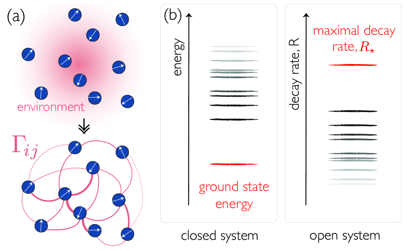
Figure 1: Generic qubit ensemble described as an out-of-equilibrium, open, many-body quantum system. (a) In Markovian baths, integrating out the environment degrees of freedom yields a spin model with coherent and dissipative interactions. The dissipative couplings between $N$ qubits are given by the decoherence matrix $\mathbf{\Gamma}=(\Gamma_{ij})_{i,j=1}^{N}$. (b) For a closed system, the ground state is the state of minimal energy. For an open system, finding the state with maximal decay rate ($R_{\star}$) is analogous to finding the ground state energy of a Hamiltonian.

Theory background. A broad class of Markovian many-body open quantum systems of $N$ qubits [Fig 1(a)] is described by the Lindblad master equation

$$\dot{\hat{\rho}}=-\frac{i}{\hbar}[\hat{H},\hat{\rho}]+\sum_{i,j=1}^{N}\Gamma_{ij}\left(\hat{\sigma}^{-}_{i}\hat{\rho}\hat{\sigma}^{+}_{j}-\frac{1}{2}\{\hat{\sigma}^{+}_{j}\hat{\sigma}^{-}_{i},\hat{\rho}\}\right),$$ (1)

where $\hat{\sigma}_{i}^{\pm}=(\hat{\sigma}_{i}^{x}\pm i\hat{\sigma}_{i}^{y})/2$ are the raising and lowering operators for qubit $i$. In the above equation, $\hat{H}$ is an arbitrary qubit Hamiltonian that commutes with the total excitation operator $\hat{n}_{\text{exc}}=\sum_{i}\hat{\sigma}^{+}_{i}\hat{\sigma}^{-}_{i}$, while the dissipative interactions are represented by the decoherence matrix $\mathbf{\Gamma}=(\Gamma_{ij})_{i,j=1}^{N}$.

For the master equation to describe a physically valid evolution (i.e., a completely positive and trace preserving map), $\mathbf{\Gamma}$ must be positive semidefinite (i.e., $\mathbf{\Gamma}\succeq 0$) [7]. This ensures non-negative eigenvalues $\{\Gamma_{\mu}\}$, which are physically interpreted as collective transition rates. Since $\mathbf{\Gamma}\succeq 0$, the spectral norm $\left\lVert\mathbf{\Gamma}\right\rVert$ is equal to $\Gamma_{\text{max}}$, the largest collective transition rate (i.e., the largest eigenvalue of the matrix). We assume $\Gamma_{ij}\in\mathbb{R}$ and $\Gamma_{ii}\equiv\Gamma_{0}\,\,\forall i$. As we discuss below, we can also account for additional terms in the master equation, such as coherent and incoherent driving, as well as disorder in $\mathbf{\Gamma}$.

The instantaneous correlated decay rate of the many-body system can be written as the expectation value of an “auxiliary” (and Hermitian) Hamiltonian $\hat{H}_{\Gamma}$ [35], i.e.,

$$R=-\frac{d}{dt}\mathinner{\langle{\hat{n}_{\text{exc}}}\rangle}\equiv\mathinner{\langle{\hat{H}_{\Gamma}}\rangle}/\hbar$$ (2)

where

$$\hat{H}_{\Gamma}=\hbar\sum_{i,j=1}^{N}\Gamma_{ij}\hat{\sigma}^{+}_{i}\hat{\sigma}^{-}_{j}=\hbar\sum_{\mu=1}^{N}\Gamma_{\mu}\hat{c}_{\mu}^{\dagger}\hat{c}_{\mu}.$$ (3)

The last equality is achieved by means of collective jump operators $\hat{c}_{\mu}=\sum_{i=1}^{N}\alpha_{i}^{(\mu)}\hat{\sigma}^{-}_{i}$, with $\alpha_{i}^{(\mu)}$ being the eigenvectors of $\mathbf{\Gamma}$ (in this notation, $\Gamma_{\text{max}}\equiv\Gamma_{1}$). Generically, the “auxiliary” Hamiltonian $\hat{H}_{\Gamma}$ describes an XY model defined on a weighted interaction graph with a local transverse field. In the specific case where the interactions are mediated by the electromagnetic field, $\mathbf{\Gamma}$ is proportional to the vacuum’s Green’s function [36, 37] and the decay rate is exactly equal to the integrated photon emission rate over all emission angles.

Lower and upper bounds. Our goal is to set theoretical limits on the maximal decay rate $R_{\star}$, which amounts to calculating the spectral radius of $\hat{H}_{\Gamma}$ (since $\hat{H}_{\Gamma}\succeq 0$), or equivalently the ground state energy of $-\hat{H}_{\Gamma}$, as depicted in Fig 1(b). Finding the exact energy is expected to be hard [15], except in two limiting cases. For non-interacting qubits (with $\Gamma_{ij}=\Gamma_{0}\delta_{i,j}$), $R_{\star}=N\Gamma_{0}$. In the Dicke limit (i.e., with all-to-all interactions such that $\Gamma_{ij}=\Gamma_{0}\;\forall\,i,j$), $R_{\star}=N(N+2)\Gamma_{0}/4$ [38, 39]. These two cases serve as trivial lower and upper bounds, respectively, for $R_{\star}$ in arbitrary environments. Below, we derive tighter product-state bounds.

Lower bound from a variational ansatz. The canonical way to obtain lower bounds on $R_{\star}$ (or equivalently, upper bounds on the ground state energy of $-\hat{H}_{\Gamma}$) is to use a variational ansatz for a trial wavefunction. We choose the product state ansatz $\mathinner{|{\psi}\rangle}=(\cos(\theta/2)\mathinner{|{g}\rangle}+\sin(\theta/2)\mathinner{|{e}\rangle})^{\otimes N}$, for which the decay rate is found to be

$$R_{\psi}(\theta)=\frac{1}{\hbar}\mathinner{\langle{\psi|\hat{H}_{\Gamma}|\psi}\rangle}=\frac{N\Gamma_{0}}{2}(1-\cos\theta)+\frac{S}{4}\sin^{2}\theta,$$ (4)

where $S\equiv\sum_{i\neq j}\Gamma_{ij}$ is the sum of dissipative interactions in the system. The maximal value of $R_{\psi}=(N\Gamma_{0}+S)^{2}/(4S)$ is attained for the mixing angle $\cos\theta=-N\Gamma_{0}/S$ if $S\geq N\Gamma_{0}$, and $\text{max}_{\psi}R_{\psi}=N\Gamma_{0}$ otherwise. Given that $-N\Gamma_{0}\leq S\leq N(N-1)\Gamma_{0}$ is necessary to satisfy $\mathbf{\Gamma}\succeq 0$ [40], our lower bound is consistent with the trivial upper bound from the Dicke model.

Modifying the ansatz to include locally-dependent relative phases between $\mathinner{|{e}\rangle}$ and $\mathinner{|{g}\rangle}$ based on the dominant eigenvector of $\mathbf{\Gamma}$ and fixing the excitation density to $1/2$ yields an alternative lower bound [see Sec. A of the Supplementary Information (SI)],

$$R_{\star}=\max_{\mathinner{|{\psi}\rangle}}\sum_{\mu}\Gamma_{\mu}\lVert{\hat{c}_{\mu}\mathinner{|{\psi}\rangle}}\rVert^{2}\geq\Gamma_{\text{max}}\lVert\hat{c}_{1}^{\dagger}\hat{c}_{1}\rVert^{2}\geq\frac{N\Gamma_{\text{max}}}{4(\Delta^{2}+1)},$$ (5)

where $0\leq\Delta\leq\sqrt{N-1}$ is the relative fluctuation of the entries of the dominant eigenvector of $\mathbf{\Gamma}$. This gives a tighter lower bound if the decay is delocalized (i.e., if the brightest collective jump operator has approximately uniform spatial support over all qubits), characterized by the regime where $\Delta=O(1)$. In particular, for a translationally-invariant system, $\Delta=0$.

Upper bound from a product state approximation. Our first main result is to find an asymptotically tighter upper bound for $R_{\star}$ by harnessing well-established theoretical guarantees for product state approximations. For many physically relevant systems, this gives us the exact scaling for $R_{\star}$ with system size. Let us write $\hat{H}_{\Gamma}=\hat{H}_{\text{diag}}+\hat{H}_{\text{XY}}$, where $\hat{H}_{\text{diag}}=\hbar\Gamma_{0}\sum_{i=1}^{N}\hat{\sigma}_{i}^{+}\hat{\sigma}_{i}^{-}$ and

$$\hat{H}_{\text{XY}}=\frac{\hbar}{4}\sum_{i\neq j}\Gamma_{ij}(\hat{\sigma}_{i}^{x}\hat{\sigma}_{j}^{x}+\hat{\sigma}_{i}^{y}\hat{\sigma}_{j}^{y}).$$ (6)

By the triangle inequality, and noting that $\|{\hat{H}_{\text{diag}}}\|=N\Gamma_{0}$, we find

$$R_{\star}\leq N\Gamma_{0}+\frac{1}{\hbar}\|\hat{H}_{\text{XY}}\|.$$ (7)

Since $\hat{H}_{\text{XY}}$ is $2$-local and traceless, we employ a recent result from Bravyi et al. [18] to write

$$\|\hat{H}_{\text{XY}}\|\leq 6\hbar\,R_{\text{prod}}(\hat{H}_{\text{XY}}),$$ (8)

where $R_{\text{prod}}(\hat{H}_{\text{XY}})$ is the best product state approximation to $\|\hat{H}_{\text{XY}}\|/\hbar$. Restricting to product states, $\hat{H}_{\text{XY}}$ reduces to a classical XY Hamiltonian

$$H_{\text{XY}}=\frac{\hbar}{4}\sum_{i\neq j}\Gamma_{ij}\vec{s}_{i}\cdot\vec{s}_{j}=\frac{\hbar}{4}\text{Tr}(\mathbf{\tilde{\Gamma}}\mathbf{\Sigma}),$$ (9)

with $\vec{s}_{i}\in\mathbb{R}^{2}$, $\left\lVert\vec{s}_{i}\right\rVert\leq 1$. In the above equation, $(\mathbf{\Sigma})_{ij}=\vec{s}_{i}\cdot\vec{s}_{j}$ is the Gram matrix for the vectors $\{\vec{s}_{i}\}$ and $\mathbf{\tilde{\Gamma}}$ is the off-diagonal matrix $\mathbf{\Gamma}-\Gamma_{0}\mathbf{I}_{N}$. By means of the inequality $\text{Tr}(\tilde{\mathbf{\Gamma}}\mathbf{\Sigma})\leq\left\lVert\mathbf{\tilde{\Gamma}}\right\rVert\text{Tr}(\mathbf{\Sigma})$ [41], we obtain

$$R_{\text{prod}}(\hat{H}_{\text{XY}})\leq\frac{N}{4}\,(\Gamma_{\text{max}}-\Gamma_{0}).$$ (10)

Combining this inequality with Eqs. (8) and  (5), we find the general bounds

$$\text{max}\left\{N\Gamma_{0},\frac{N\Gamma_{\text{max}}}{4(\Delta^{2}+1)}\right\}\leq R_{\star}\leq\frac{N}{2}\left(3\Gamma_{\text{max}}-\Gamma_{0}\right).$$ (11)

For the upper bound, equality is achieved for non-interacting qubits ($\Gamma_{\text{max}}=\Gamma_{0}$). Equation (11) also implies that for ‘sufficiently weak’ interactions such that $\Gamma_{\text{max}}$ is asymptotically independent of $N$, the maximal decay rate scales only linearly with system size. This generalizes some of the authors’ recent results on the impossibility of Dicke superradiance with nearest-neighbor interactions [35], to systems with arbitrary interaction range and geometry.

While the use of the product state approximation is not strictly needed to obtain an upper bound on $R_{\star}$, it provides several advantages. Physically, it implies that entanglement is not necessary for a system to dissipate at a rate near the theoretical maximum scaling, complementary to previous observations about the role of entanglement in spontaneous transient superradiance [42, 43, 44]. Furthermore, this formalism can be extended to yield upper bounds on the rates of change of higher-order observables such as $k$-point correlation functions. Here, the “auxiliary” Hamiltonian will in general be $(k+1)$-local, and the optimal product state provides an approximation with a multiplicative error of at most $3^{k+1}$, independent of system size [18].

Universal scaling laws. Our bounds are tight for systems with delocalized decay (differing only by a constant factor), thus yielding scaling laws for the maximal decay rate. Taking $\Delta=O(1)$ in Eq. (11), we find

$$R_{\star}\sim N\Gamma_{\text{max}},$$ (12)

which is one of the main results of this paper. The scaling law $R_{\star}\sim N\Gamma_{\text{max}}$ in the delocalized regime is non-trivial and certainly not true for arbitrary systems. More broadly, in Sec. B of SI we prove that there are no general scaling laws on $R_{\star}$ that depend solely on system size and the spectrum of $\mathbf{\Gamma}$. Since $\Gamma_{\text{max}}$ can be computed numerically in $O(N^{3})$ time, the scaling law provides an efficient scheme to approximate $R_{\star}$ for large system sizes with quasi translation invariance (i.e., such that $\Delta=O(1)$). As discussed in Sec. C of SI, these scaling laws are robust to disorder in $\mathbf{\Gamma}$, and hold even in the presence of any number of local Hamiltonian and dissipative terms. We can also extend our formalism to treat coherent and incoherent driving, dephasing, and multi-qubit interactions, without affecting the scaling.

This scaling law reduces to the limiting trivial cases of independent decay (where $\Gamma_{\text{max}}=\Gamma_{0}$ and thus $R_{\star}\sim N\Gamma_{0}$) and of all-to-all interactions in the Dicke limit (where $\Gamma_{\text{max}}=N\Gamma_{0}$, and $R_{\star}\sim N^{2}\Gamma_{0}$). The latter reveals important insights about the $N^{2}$ scaling in superradiant systems: one factor of $N$ arises from the approximate permutation symmetry, and the other from the delocalized nature of the dominant decay channel together with a non-vanishing excitation density at large $N$.

It may seem surprising that a product state yields the same asymptotic decay rate as the highly-entangled Dicke state, but this can be thought of as an instance of the quantum de Finetti theorem [45, 46]: Since $\hat{H}_{\Gamma}$ is $2$-local, it suffices to only consider the two-body reduced density matrix of the permutationally symmetric Dicke state, which is close to a product state (with trace distance vanishing as $1/N$). Our results show that the accuracy of the mean field (product state) ansatz holds more generally, even when the permutation symmetry is broken.

Maximal decay rate of atomic arrays in free space. Interactions between atoms are mediated by different types of photons, typically ranging from optical to microwave. Here we focus on ordered lattices of two-level atoms, whose interactions are described by the propagator of the electromagnetic field evaluated at the resonance frequency $\omega_{0}$, which is a long-ranged function with oscillating sign (see Sec. D of SI). This makes the problem of finding the ground state of $-\hat{H}_{\Gamma}$ non-trivial, and is thus a perfect candidate to showcase the strength of our theoretical tools. We note that our formalism is not restricted to electric-dipole-mediated interactions in free space, but can also describe magnetic-dipole or electric-quadrupole interactions in arbitrarily complex dielectric structures.

In the large $N$ limit, and for a large range of lattice constants, the functional dependence on system size of the largest transition rate is only determined by the dimensionality of the array [47]. One can relate the scaling with $N$ to the presence of divergences of $\Gamma(\textbf{k})$ in reciprocal space as $|\textbf{k}|$ approaches $k_{0}\equiv\omega_{0}/c$. Divergences do not occur for one-dimensional (1D) arrays. They appear for two- and three-dimensional (2D, 3D) lattices, as the number of atoms per volume increases, enhancing constructive interference of photon emission for certain wavevectors. For a D-dimensional array, the largest transition rate scales as $\Gamma_{\text{max}}^{\text{(D)}}/\Gamma_{0}\sim(k_{0}d)^{-\frac{\text{D+1}}{2}}N^{\frac{\text{D-1}}{\text{2D}}}$(see SI). Since the collective jump operators are extended, Eq. (12) holds, allowing us to derive a scaling law for $R_{\star}$.

The asymptotic scaling of the maximal decay rate depends on the array dimensionality (D $\in\{1,2,3\}$) as

$$\frac{R_{\star}^{\text{(D)}}}{\Gamma_{0}}\sim N^{\frac{3}{2}-\frac{1}{2\text{D}}}.$$ (13)

This expression, which is one of the main results of the paper, is universal in the sense that it does not depend on microscopic details (such as lattice constant, geometry, polarization), which only appear as prefactors that do not change the scaling as long as the atom number is large enough. The scaling law differs significantly from that expected in the Dicke limit as $N\to\infty$. The departure is largest for 1D arrays, which effectively scale as a collection of non-interacting atoms.

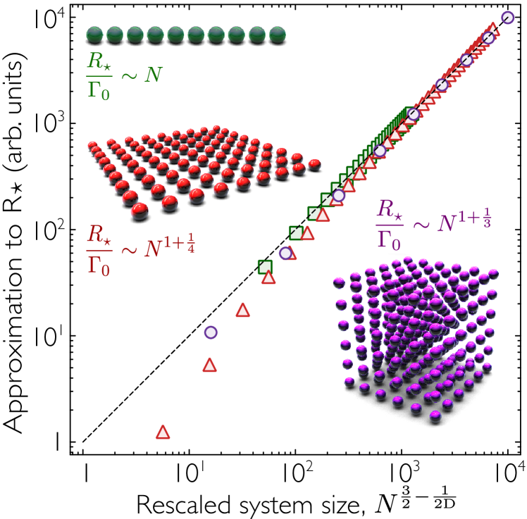
Figure 2: Scaling with system size of the numerical approximation for the maximal decay rate $R_{\star}$ given by the SDP solution, for different lattice dimensionalities with lattice constant $d=0.4\lambda_{0}$. For 1D ($\square$) and 2D ($\triangle$) arrays, the atoms are perpendicularly polarized; for the 3D ($\circ$) lattice, the atoms are polarized along one axis of the array. The dashed black line represents the analytical scaling law $R_{\star}\sim N^{\frac{3}{2}-\frac{1}{\text{2D}}}\Gamma_{0}$.

We benchmark our analytical scaling laws via a semidefinite program (SDP) relaxation [48], which provides an upper bound to $R_{\text{prod}}(\hat{H}_{\text{XY}})$ [see Eqs. (8) and (9)]. SDP relaxations have been used to lower-bound different types of ground state problems [49, 50, 51, 52] and, more recently, ground-state observables [53]. The SDP relaxation to Eq. (9) reads

$$\begin{split}\max_{\mathbf{X}\succeq 0,\mathbf{X}^{T}=\mathbf{X}}\quad&\frac{1}{4}\text{Tr}(\mathbf{\tilde{\Gamma}}\mathbf{X})\\ \text{subject to}\quad&\mathbf{X}_{ii}\leq 1\quad\forall i=1,\ldots,N\end{split}$$ (14)

which can be solved in polynomial time. Here, $\mathbf{X}$ is the Gram matrix with elements $\mathbf{X}_{ij}=\vec{x}_{i}\cdot\vec{x}_{j}$, $\vec{x}_{i}\in\mathbb{R}^{N}$. This is a relaxation since the Gram matrix $\mathbf{\Sigma}$ associated to $R_{\text{prod}}(\hat{H}_{\text{XY}})$ has a rank of at most $2$, while $\mathbf{X}$ can have a rank of up to $N$. Relaxing the rank constraint renders the optimization problem convex, and thus efficiently solvable. Using an SDP solver [54], we obtain a good approximation of $R_{\star}$ as shown in Fig. 2 for arrays with lattice constant $d=0.4\lambda_{0}$, where $\lambda_{0}=2\pi/k_{0}$ is the wavelength associated to the resonant transition.

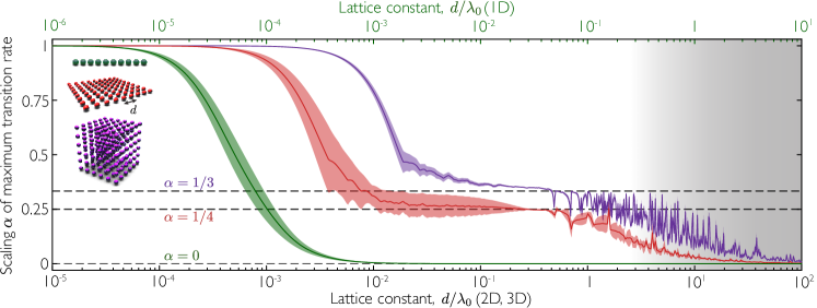
Figure 3: Finite size effects in the scaling of the largest transition rate (obtained from a best fit to $\Gamma_{\text{max}}=\beta N^{\alpha}\Gamma_{0}$) as a function of lattice constant. The atoms form a square lattice and are polarized parallel to one axis of the array. The fits are done over a region $N_{\text{1D}}\in[2,N^{\text{max}}_{\text{1D}}]$, where $N^{\text{max}}_{\text{1D}}=\{30000,250,40\}$ for 1D, 2D, and 3D, respectively. The colored regions represent the 1$\sigma$ confidence interval. The gray area shows the region where the fit is not accurate (R-squared $<0.95$, see Sec. D of SI). The upper axis shows the lattice constant exclusively for 1D arrays. Dashed lines represent the analytical scaling.

For large $N$, the numerical approximations to $R_{\star}$ given by the SDP follow the analytical scaling law of Eq. (13). For visualization purposes, we shift the data set corresponding to each lattice dimension by a multiplicative factor (a constant upward shift in logarithmic scale). These shifts do not affect the scaling and highlight the excellent agreement between the numerical results and the analytical scaling laws. Our results suggest that the SDP can be a valuable tool to obtain empirical scaling laws of $R_{\star}$ at large system sizes for more complicated systems that are analytically intractable. We further verify our results numerically via exact diagonalization of $\hat{H}_{\Gamma}$ for 1D and 2D arrays in Sec. E of SI.

For sufficiently large atom numbers the scalings hold regardless of the lattice constant. For finite $N$, however, they depend on other parameters such as the lattice constant and lateral size $L=N^{1/D}d$, as shown in Fig. 3. As we discuss in the SI, by taking the limits of the expression for $\mathbf{\Gamma}$ in the appropriate order ($k_{0}d\rightarrow 0$ before $N\rightarrow\infty)$ we confirm that for $L\ll\lambda_{0}$, one recovers Dicke’s scaling, i.e., $\Gamma_{\text{max}}=N\Gamma_{0}$. For arrays with large lattice constant, $d\gg\lambda_{0}$, following a similar procedure yields the limit of non-interacting atoms, i.e., $\Gamma_{\text{max}}\simeq\Gamma_{0}$. We determine the crossover between “non-interacting” and “collective” behaviors by identifying the parameters for which there is an asymptotic change in the scaling of $R_{\star}$, from linear to superlinear. For 2D and 3D arrays the number of atoms required for such crossover is $N^{\text{(crit)}}\simeq\eta(k_{0}d)^{6}$, where $\eta=0.02$ and $5$, respectively. As expected, for large inter-particle distances the number of atoms required for $R_{\star}$ to be superlinear grows rapidly.

Discussion and outlook. Our findings on the scaling of $R_{\star}$ crucially address fundamental problems in quantum optics, such as transient and steady-state superradiance in extended systems [38, 39, 55]. Beyond the cavity or Dicke limit, questions about scalings with system size have remained elusive, having often been addressed through numerical approximations [56, 57]. Since the decay rate is directly connected to the intensity of the emitted light, $R_{\star}$ sets rigorous upper bounds on the scaling of the superradiant burst. While this upper bound may be violated if light is collected only over a small solid angle, new scaling laws can be derived taking into account the detector aperture. We anticipate that our results will also play a role in determining the presence of quantum phase transitions, such as those of the superradiant laser [2, 3] or the driven Dicke model [4, 5, 6].

Our results open the door to finding optimal schemes for metrology protocols. Recent experiments on lattice clocks [31] and spin squeezing [58, 32, 33, 34] have investigated the role of Hamiltonian power-law dipole-dipole interactions. The dissipative counterpart of the interaction is typically neglected (as dephasing noise is currently the main source of error), although it sets a fundamental limit on the time available to generate and utilize metrologically-useful states. Nevertheless, there should be configurations (i.e., lattice dimension, lattice constant, and interrogation scheme) that enhance Hamiltonian interactions and suppress correlated decay, potentially benefiting magnetometry as well [59]. More sophisticated methods include tailoring the Green’s function of the environment via dielectric structures such as photonic crystals.

The scaling law (13) indicates that correlated decay may hamper quantum error correction [60, 61, 9], as the error rate per qubit scales (in the worst case) as $\sim R_{\star}/N$, which grows with $N$ in 2D and above. Nevertheless, in Sec. F of SI, we prove that the decay rate for typical (Haar-random) states is close to $N\Gamma_{0}/2$. Therefore, most states in the Hilbert space do not experience correlated decay, due to random phases between the qubits. This does not mean that the scaling laws for $R_{\star}$ are irrelevant in practice, since even simple states like the product state $\mathinner{|{+}\rangle}^{\otimes N}$ may be superradiant.

In experimental implementations with Rydberg arrays, correlated decay may increase leakage error rates out of the computational subspace [62]. Our results predict that collective decay becomes relevant for $N\gtrsim(2\pi\eta^{1/6}L/\lambda_{0})^{6\text{D}/(\text{D}+6)}$. For atoms trapped in optical lattices and tweezer arrays, $L\approx 1\,\text{mm}$, limited by the field of view of the objective. For optical transitions (with $\lambda_{0}\approx 1\,\mu$m) we estimate that decay can become collectively enhanced for $N\gtrsim 10^{5}$ in 2D and $10^{7}$ in 3D arrays (state-of-the art experiments have reported $N\sim 6000$ [63]). For microwave transitions, such as between Rydberg states (where $\lambda_{0}\approx 10\,\text{mm}$), even tiny 2D and 3D arrays lie within the collective decay regime. Nevertheless, the number of atoms for which $R_{\star}>N\Gamma_{0}$ scales as $\sim(k_{0}d)^{6}$ for both 2D and 3D arrays. Therefore, it is possible to suppress correlated decay by increasing the lattice constant, at the cost of increased gate time.

Finally, our results demonstrate the broad potential of quantum approximation techniques to predict relevant properties of open many-body systems. Our approach could be adapted to study the steady-state behavior of driven-dissipative systems, and to predict the scaling of correlations functions or other physical observables [53]. More advanced SDP relaxations such as the quantum Lasserre hierarchy [52] could yield tighter bounds for generic systems. These methods are not restricted to spin models, and could be extended to study ensembles of interacting fermions or bosons, as well as to disordered systems. Moreover, invoking time-reversal arguments, our scalings also apply to the maximal absorption rate, which may have implications for quantum batteries [64] and light harvesting protocols [65]. Given their generality, we anticipate that these ideas will become a powerful tool to investigate universal properties of large scale many body open quantum systems.

Acknowledgments. We thank Antonio Acin, Paul R. Berman, Darrick E. Chang, Tobias Haug, Simon B. Jäger and Leo Zhou for helpful discussions. We are grateful to Silvia Cardenas-Lopez for her help with the design of the first figure. We acknowledge support by the National Science Foundation through the CAREER Award (No. 2047380), the Air Force Office of Scientific Research through their Young Investigator Prize (grant No. 21RT0751), as well as by the David and Lucile Packard Foundation. JP acknowledges support from the National Science Foundation (Award No. PHY-2317110). The Institute for Quantum Information and Matter is an NSF Physics Frontiers Center.

Supplementary Information

A Lower bound for delocalized decay

By means of the variational principle and Eq. (3) we find

$$R_{\star}=\max_{\mathinner{|{\psi}\rangle}}\sum_{\mu}\Gamma_{\mu}\lVert\hat{c}_{\mu}\mathinner{|{\psi}\rangle}\rVert^{2}\geq\Gamma_{\text{max}}\lVert\hat{c}_{1}^{\dagger}\hat{c}_{1}\rVert.$$ (15)

Substituting the definition of the collective operators $\hat{c}_{\mu}$, we arrive at

$$\begin{split}R_{\star}&\geq\Gamma_{\text{max}}\bigg{\|}\sum_{i,j}\alpha_{i}^{(1)*}\alpha_{j}^{(1)}\hat{\sigma}_{i}^{+}\hat{\sigma}_{j}^{-}\bigg{\|}=\Gamma_{\text{max}}\bigg{\|}\sum_{i,j}\left|\alpha_{i}^{(1)}\right|\left|\alpha_{j}^{(1)}\right|\tilde{\sigma}_{i}^{+}\tilde{\sigma}_{j}^{-}\bigg{\|}=\Gamma_{\text{max}}\max_{\mathinner{|{\psi}\rangle}}\sum_{i,j}\left|\alpha_{i}^{(1)}\right|\left|\alpha_{j}^{(1)}\right|\mathinner{\langle{\psi|\tilde{\sigma}_{i}^{+}\tilde{\sigma}_{j}^{-}|\psi}\rangle}\\ &\geq\frac{\Gamma_{\text{max}}}{4}\left(\sum_{i}\left|\alpha_{i}^{(1)}\right|\right)^{2},\end{split}$$ (16)

where we have absorbed the phases $\phi_{i}$ of $\alpha_{i}^{(1)}$ into the lowering operators $\tilde{\sigma}_{i}^{-}=e^{i\phi_{i}}\hat{\sigma}_{i}^{-}$. The last inequality is obtained by choosing the product state $\mathinner{|{\psi}\rangle}=\bigotimes_{i}(\mathinner{|{g}\rangle}+\exp(-i\phi_{i})\mathinner{|{e}\rangle})_{i}/\sqrt{2}$ such that $\mathinner{\langle{\psi|\tilde{\sigma}_{i}^{+}\tilde{\sigma}_{i}^{-}|\psi}\rangle}=1/2$. The lower bound thus depends on how the collective operator $\hat{c}_{1}$ is spatially supported on the $N$ qubits, quantified by the variance of $|\alpha_{i}^{(1)}|$, which reads

$$\begin{split}\text{Var}(|\alpha^{(1)}|)&=\frac{1}{N}\sum_{i}\left(\left|\alpha_{i}^{(1)}\right|-\overline{\left|\alpha^{(1)}\right|}\right)^{2}=\frac{1}{N}-\frac{1}{N^{2}}\left(\sum_{i}\left|\alpha_{i}^{(1)}\right|\right)^{2}.\end{split}$$ (17)

The second line of the equation is obtained by using $\sum_{i}|\alpha_{i}^{(1)}|^{2}=1$, and $\overline{|\alpha^{(1)}|}=\sum_{i}\left|\alpha_{i}^{(1)}\right|/N$. Defining the relative fluctuation of $|\alpha_{i}^{(1)}|$ as $\Delta=\sqrt{\text{Var}(\left|\alpha^{(1)}\right|)}/\overline{\left|\alpha^{(1)}\right|}$ yields Eq. (5). Explicitly,

$$\Delta^{2}=\frac{N}{\left\lVert\vec{\alpha}^{(1)}\right\rVert_{1}^{2}}-1,$$ (18)

where $\vec{\alpha}^{(1)}=(\alpha_{1}^{(1)}\ldots\alpha_{N}^{(1)})^{T}$ is the dominant eigenvector of $\mathbf{\Gamma}$, and $\left\lVert\vec{\alpha}^{(1)}\right\rVert_{p}$ is the $L^{p}$ vector norm. Using the inequality $\left\lVert\vec{\alpha}^{(1)}\right\rVert_{2}\leq\left\lVert\vec{\alpha}^{(1)}\right\rVert_{1}\leq\sqrt{N}\left\lVert\vec{\alpha}^{(1)}\right\rVert_{2}$ and $\left\lVert\vec{\alpha}^{(1)}\right\rVert_{2}=1$ by normalization, we have the bound

$$0\leq\Delta\leq\sqrt{N-1}.$$ (19)

The upper bound $\Delta=\sqrt{N-1}$ is satisfied for independent emitters. Intuitively, $\Delta$ quantifies the spatial uniformity of the brightest collective jump operator $\hat{c}_{1}$. Thus, we define the delocalized decay regime to be $\Delta=O(1)$. For translationally invariant systems, $|\alpha_{i}^{(\mu)}|=N^{-1/2}$ for all $i=1,\ldots,N$ and $\mu=1,\ldots,N$, such that $\Delta=0$.

B No scaling law in the absence of delocalized decay

The scaling law $R_{\star}\sim N\Gamma_{\text{max}}$ derived for systems in the delocalized regime is not true for arbitrary systems. We now prove that no general scaling law exists that depend solely on $N$ and the spectrum of $\mathbf{\Gamma}$. This can be seen by reductio ad absurdum. Let us suppose $R_{\star}\sim f(N)g(\Gamma_{1},\ldots,\Gamma_{N})$, where $f$ and $g$ are arbitrary functions. By applying an orthogonal transformation on $\mathbf{\Gamma}$, one can obtain a diagonal decoherence matrix $\mathbf{\Gamma^{\prime}}=\text{diag}(\Gamma_{1},\ldots,\Gamma_{N})$. Since $\mathbf{\Gamma^{\prime}}$ has the same spectrum as $\mathbf{\Gamma}$, the new maximal decay rate $R_{\star}^{\prime}\sim R_{\star}$ by assumption. However, $\mathbf{\Gamma^{\prime}}$ physically describes a system of $N$ independent qubits with decay rates $\Gamma_{1},\ldots,\Gamma_{N}$, respectively. Hence, $R_{\star}^{\prime}=\sum_{i}\Gamma_{i}=N\Gamma_{0}$ which is not $\sim R_{\star}$ in general. Thus, by contradiction, a general scaling law for $R_{\star}$ of the form $f(N)g(\Gamma_{1},\ldots,\Gamma_{N})$ does not exist, without assumptions on the system. This does not invalidate our scaling law for translationally invariant systems, as orthogonal transformations of $\mathbf{\Gamma}$ generally break translation symmetry.

C Effect of disorder, local and non-local Hamiltonian and dissipative terms

Here, we show that our scaling law $R_{\star}\sim N\Gamma_{\text{max}}$ holds much more generally than under the assumptions we considered in Eq. (1).

C.1 Disorder

We include disorder by considering a decoherence matrix

$$\mathbf{\Gamma}^{\prime}=\mathbf{\Gamma}+\mathbf{\Gamma}_{\text{disorder}},$$ (20)

with the disorder matrix $\mathbf{\Gamma}_{\text{disorder}}$ Hermitian but not positive semidefinite in general. For the decoherence matrix to be physically valid, we demand that $\mathbf{\Gamma}^{\prime}\succeq 0$. Weyl’s inequality (see p. 239 of Ref. Horn_Johnson_2012) yields

$$\left|R_{\star}^{\prime}-R_{\star}\right|\leq\left\lVert\hat{H}_{\Gamma_{\text{disorder}}}\right\rVert$$ (21)

and

$$\left|\Gamma^{\prime}_{\text{max}}-\Gamma_{\text{max}}\right|\leq\left\lVert\mathbf{\Gamma}_{\text{disorder}}\right\rVert,$$ (22)

where $R^{\prime}_{*}$ and $\Gamma^{\prime}_{\text{max}}$ are the new maximal decay rate and largest transition rate respectively. $\hat{H}_{\Gamma_{\text{disorder}}}$ is defined analogously to Eq. (3) with the decoherence matrix $\mathbf{\Gamma_{\text{disorder}}}$. This shows that the scaling of $R_{\star}$ is unchanged if $\left\lVert\mathbf{\Gamma}_{\text{disorder}}\right\rVert<R_{\star}$. Also, if $\left\lVert\mathbf{\Gamma}_{\text{disorder}}\right\rVert<\Gamma_{\text{max}}$ (in the large $N$ limit), this is sufficient to ensure that $\Gamma^{\prime}_{\text{max}}$ and $\Gamma_{\text{max}}$ have the same scaling with $N$, so the scaling for the general upper bound on $R_{\star}$ remains unchanged. In the delocalized decay regime where $\Delta=O(1)$, Eqs. (5) and (11) also imply that $R_{\star}\propto N\Gamma_{\text{max}}$ even in the presence of disorder, at least up to $\left\lVert\mathbf{\Gamma}_{\text{disorder}}\right\rVert=\Gamma_{\text{max}}$.

C.2 Local Hamiltonian and dissipation

We consider a general $k$-local qubit Hamiltonian $H^{(k)}$ which can be written as a linear combination of $Q$ Pauli strings of weight $k$

$$\hat{H}^{(k)}=\hbar\sum_{j=1}^{Q}\eta_{j}\hat{P}_{j}^{(k)}.$$ (23)

Each $\hat{P}_{j}^{(k)}$ is a tensor product of $k$ single-qubit (non-identity) Pauli operators acting on $k$ qubits, and act identically on the remaining $N-k$ qubits. The coefficients $\eta_{j}\in\mathbb{R}$ are constants assumed to be independent of $N$, i.e., proportional to $\Gamma_{0}$. On top of that, we can also add $Q$ independent $k$-local dissipation channels denoted by Lindblad dissipators of the form

$$\sum_{j=1}^{Q}\kappa_{j}(\hat{P}_{j}^{(k)}\hat{\rho}\hat{P}_{j}^{(k)}-\hat{\rho}),$$ (24)

where we have used the fact that the Pauli strings $\hat{P}_{j}^{(k)}$ satisfy $\hat{P}_{j}^{(k){\dagger}}=\hat{P}_{j}^{(k)}$ and $\hat{P}_{j}^{(k)2}=1$ to simplify the expression. The rates $\kappa_{j}$ are positive coefficients that we assume to be independent of $N$. Physically, $\kappa_{j}$ represents the decay rate of the local dissipative channel with jump operator $\hat{P}_{j}^{(k)}$. Adding these terms modify the master equation (1) to

$$\dot{\hat{\rho}}=-\frac{i}{\hbar}[\hat{H}+\hat{H}^{(k)},\hat{\rho}]+\sum_{i,j=1}^{N}\Gamma_{ij}\left(\hat{\sigma}^{-}_{i}\hat{\rho}\hat{\sigma}^{+}_{j}-\frac{1}{2}\{\hat{\sigma}^{+}_{j}\hat{\sigma}^{-}_{i},\hat{\rho}\}\right)+\sum_{j=1}^{Q}\kappa_{j}(\hat{P}_{j}^{(k)}\hat{\rho}\hat{P}_{j}^{(k)}-\hat{\rho}).$$ (25)

We now bound the contributions of the additional Hamiltonian and dissipative terms to the decay rate $R$. First, let us examine the contribution of the local Hamiltonian $H^{(k)}$. From the expression $\hat{n}_{\text{exc}}=\sum_{i=1}^{N}(\mathbf{I}_{2}+\hat{\sigma}_{i}^{z})/2$,

$$R=-\frac{i}{2}\sum_{j=1}^{Q}\eta_{j}\mathinner{\langle{[\hat{P}_{j}^{(k)},\sum_{i=1}^{N}\hat{\sigma}_{i}^{z}]}\rangle}.$$ (26)

The commutator term produces a linear combination of at most $k$ Pauli strings, since each $\hat{P}_{j}^{(k)}$ is supported only on $k$ qubits. Using the fact that the expectation value of a Pauli string has a magnitude of at most $1$, we obtain the bound

$$R\leq\text{const.}\times k\sum_{j=1}^{Q}|\eta_{j}|=O(kQ\Gamma_{0}).$$ (27)

Next, we examine the contribution from the local dissipation:

$$R=\sum_{j=1}^{Q}\kappa_{j}\left(\mathinner{\langle{\hat{n}_{\text{exc}}}\rangle}-\mathinner{\langle{\hat{P}_{j}^{(k)}\hat{n}_{\text{exc}}\hat{P}_{j}^{(k)}}\rangle}\right)=\sum_{j=1}^{Q}\frac{\kappa_{j}}{2}\sum_{i=1}^{N}\left(\mathinner{\langle{\hat{\sigma}_{i}^{z}}\rangle}-\mathinner{\langle{\hat{P}_{j}^{(k)}\hat{\sigma}_{i}^{z}\hat{P}_{j}^{(k)}}\rangle}\right).$$ (28)

The term in the parenthesis has a non-vanishing contribution if qubit $i$ lies within the support of $\hat{P}_{j}^{(k)}$. A similar argument as before gives the bound

$$R\leq\text{const.}\times k\sum_{j=1}^{Q}\kappa_{j}=O(kQ\Gamma_{0}).$$ (29)

The upshot is that adding the local Hamiltonian and dissipative terms can only contribute an $O(kQ\Gamma_{0})$ correction to the decay rate and thus

$$R_{\star}\sim N\Gamma_{\text{max}}+O(kQ\Gamma_{0}).$$ (30)

The size of this correction depends on $k$ and $Q$. Of course, if we include all possible choices of $k$-local Pauli strings, $Q=3^{k}\binom{N}{k}$ dominates over the scaling of $N\Gamma_{\text{max}}$ for $k\geq 2$. However, a vast majority of such Pauli strings contain spatially non-local interactions. We impose geometric locality on $\hat{P}_{j}^{(k)}$ by demanding that each of the $k$ qubits involved are located within a $D$-dimensional ball of constant radius $r$. For an ordered system in $D$ spatial dimensions, we have $Q=O(\text{const.}^{k}\times Nr^{kD}/k!)$, where the constant comes from the $3^{k}$ choices of Pauli operators and also other geometrical factors (such as the coordination number). As long as the locality $k$ of the interaction is independent of the system size, the correction to $R_{\star}$ is only linear in $N$, which does not affect our scaling laws. We remark that a lattice geometry is not strictly necessary here, and a similar counting argument for $Q$ can be made for a spatially disordered system of qubits as long as the interactions described by $\hat{P}_{j}^{(k)}$ remain spatially local.

C.3 Driven-dissipative systems

One can generalize Eq. (1) to include both coherent and incoherent drives, described by the master equation

$$\begin{split}\dot{\hat{\rho}}&=-i\left[\hat{H}+\sum_{j}(\eta_{j}\hat{\sigma}^{+}_{j}+\text{h.c.}),\hat{\rho}\right]+\sum_{i,j=1}^{N}\Gamma_{ij}\left(\hat{\sigma}^{-}_{i}\hat{\rho}\hat{\sigma}^{+}_{j}-\frac{1}{2}\{\hat{\sigma}^{+}_{j}\hat{\sigma}^{-}_{i},\hat{\rho}\}\right)+\sum_{i,j=1}^{N}W_{ij}\left(\hat{\sigma}^{+}_{i}\hat{\rho}\hat{\sigma}^{-}_{j}-\frac{1}{2}\{\hat{\sigma}^{-}_{j}\hat{\sigma}^{+}_{i},\hat{\rho}\}\right),\end{split}$$ (31)

where the coherent and incoherent driving strengths are given by the constants $\eta_{j}$ and $W_{ij}$, respectively. The incoherent terms can arise from both an external pump or a finite temperature reservoir, allowing for the possibility of collective pumping. The instantaneous correlated many-body decay rate in Eq. (2) now becomes $R=\langle\hat{H}_{\Gamma}\rangle+\langle V_{W}\rangle+\langle V_{\eta}\rangle$ where

$$V_{W}=-\sum_{i,j}W_{ij}\hat{\sigma}^{+}_{i}\hat{\sigma}^{-}_{j}+\sum_{j=1}^{N}W_{jj}\hat{\sigma}^{z}_{j},\;\;\text{and}\;\,V_{\eta}=i\sum_{j=1}^{N}(\eta_{j}\hat{\sigma}^{+}_{j}-\text{h.c.}).$$ (32)

Assuming non-extensive parameters, both $V_{\eta}$ and the second term in $V_{W}$ can only shift $R_{\star}$ by at most $O(N)$ (see Section C.2), which does not affect the scaling of $R_{\star}$. Thus, it suffices to consider the shifted decoherence matrix $\mathbf{\Gamma}-\mathbf{W}$ arising from incoherent pumping, where $\mathbf{W}=(W_{ij})_{i,j=1}^{N}$, as $R_{\star}$ is asymptotically equivalent to the largest eigenvalue of $\hat{H}_{\Gamma-W}$. One can thus identify the pumping with an effective disorder, and associate $\mathbf{\Gamma}_{\text{disorder}}\equiv-\mathbf{W}$, which implies that the scaling of $R_{\star}$ is unaffected if $\left\lVert V_{W}\right\rVert<R_{\star}$. Similarly, the scaling of $\Gamma_{\text{max}}$ is unaffected if $\left\lVert\mathbf{W}\right\rVert<\Gamma_{\text{max}}$.

For a finite temperature reservoir, $\mathbf{\Gamma}-\mathbf{W}$ is independent of the mean number of thermal bosons $\bar{n}_{\text{th}}$ in the reservoir Carmichael1993open. Thus, assuming that $\bar{n}_{\text{th}}$ does not scale with $N$ such that the second term in $V_{W}$ only contributes at most $O(N)$ to $R_{\star}$, the scaling of $R_{\star}$ is equivalent to that of a zero-temperature bath. This indicates that our scaling laws obtained from the analysis of Eq. (1) remain valid even at finite temperatures and, more generally, for driven-dissipative systems, except for very strong driving strengths where $\left\lVert V_{W}\right\rVert$ or $\left\lVert V_{\eta}\right\rVert$ scale faster than $R_{\star}/N$.

D Scaling of the largest transition rate for atomic arrays in free space

We consider ensembles of $N$ two-level atoms arranged in 1D, 2D and 3D ordered arrays with lattice constant $d$. Tracing out the vacuum electromagnetic modes within the Born-Markov approximation, one obtains an effective master equation for the atomic dynamics of the same form as Eq. (1) Lehmberg1970aSupp. Here, the atom-atom dissipative coupling rates read AsenjoGarcia2017PRXSupp

$$\Gamma_{ij}=\frac{6\pi\Gamma_{0}}{k_{0}}\hat{\bm{\wp}}^{*}\cdot\text{Im}\,\textbf{G}(\textbf{r}_{i},\textbf{r}_{j},\omega_{0})\cdot\hat{\bm{\wp}},$$ (33)

where $\omega_{0}=ck_{0}$ is the atomic resonance frequency, $\Gamma_{0}=\omega_{0}^{3}|\bm{\wp}|^{2}/3\pi\hbar\epsilon_{0}c^{3}$ is the single-atom spontaneous emission rate, and $\bm{\wp}$ is the dipole matrix element of the atomic transition. The dissipative couplings between atoms $i$ and $j$ are given by the imaginary part of the field propagator between them (projected in the direction of the atomic transition dipole element), $\textbf{G}(\textbf{r}_{i},\textbf{r}_{j},\omega_{0})\equiv\textbf{G}(\textbf{r}_{ij},\omega_{0})$, where $\textbf{r}_{ij}=\textbf{r}_{i}-\textbf{r}_{j}$ is the relative position between the atoms. In 3D vacuum, the electromagnetic Green’s tensor reads jackson

$$\begin{split}\textbf{G}(\textbf{r},\omega_{0})\equiv&\frac{e^{{\rm i}k_{0}r}}{4\pi k_{0}^{2}r^{3}}\Big{[}(k_{0}^{2}r^{2}+{\rm i}k_{0}r-1)\mathds{1}+(-k_{0}^{2}r^{2}-3{\rm i}k_{0}r+3)\frac{\textbf{r}\otimes\textbf{r}}{r^{2}}\Big{]},\,\,\,\text{where}\,\,r=|\textbf{r}|.\end{split}$$ (34)

For ordered atomic arrays, the scaling of $R_{\star}$ with system size is entirely determined by $N\Gamma_{\text{max}}$, as shown by Eq. (12). In this section, we find analytical expressions for the scaling of $\Gamma_{\text{max}}$ with system size. To do so, we go to momentum space (assuming large atom number). The collective transition rates read

$$\Gamma(\mathbf{k})=\frac{6\pi\Gamma_{0}}{k_{0}}\hat{\bm{\wp}}^{*}\cdot\text{Im}\,\tilde{\textbf{G}}(\mathbf{k})\cdot\hat{\bm{\wp}},$$ (35)

where $\tilde{\textbf{G}}(\mathbf{k})=\sum_{j}e^{-i\mathbf{k}\cdot{\bf r}_{j}}\textbf{G}({\bf r}_{j},\omega_{0})$ is the Fourier transform of the Green’s function in Eq. (34). Below we study potential divergences of the “imaginary” dispersion relation in the Brillouin zone. We provide a route to connect them with finite size scalings by expressing the largest transition rate as $\Gamma_{\text{max}}=\beta N^{\alpha}\Gamma_{0}$. These scalings also depend on the order of the limits $N\rightarrow\infty$ and $k_{0}d\rightarrow 0$ (or $k_{0}d\rightarrow\infty$), which we also discuss.

D.1 1D arrays

The transition rate of a spin wave with momentum $k_{z}$ can be computed directly from Eq. (35) and reads AsenjoGarcia2017PRXSupp

$$\begin{split}\frac{\Gamma_{\text{1D}}^{\parallel}(k_{z})}{\Gamma_{0}}&=\frac{3\pi}{2k_{0}d}\sum_{g_{z}}\left(1-\frac{(k_{z}+g_{z})^{2}}{k_{0}^{2}}\right),\\ \frac{\Gamma_{\text{1D}}^{\perp}(k_{z})}{\Gamma_{0}}&=\frac{3\pi}{4k_{0}d}\sum_{g_{z}}\left(1+\frac{(k_{z}+g_{z})^{2}}{k_{0}^{2}}\right),\end{split}$$ (36)

where the summation runs over reciprocal lattice vectors $g_{z}=2\pi n/d$ for $n\in\mathbb{Z}$ that satisfy the condition $|g_{z}+k_{z}|\leq k_{0}$. Here, the superscripts $\{^{\parallel},^{\perp}\}$ refer to atoms with polarization parallel and perpendicular to the array, respectively.

For a finite lattice constant $d$, the transition rates do not scale with $N$ and $\beta^{\text{(1D)}}\sim 1/k_{0}d$. The lack of divergence in reciprocal space can be understood as follows. Let us take the limit of large lattice constant in Eq. (36), where the sum over reciprocal lattice vectors extends up to $g_{\text{max}}=2\pi n_{*}/d$, where $n_{*}=d/\lambda_{0}$. Computing the sums in Eq. (36) in the limit $d/\lambda_{0}\gg 1$ one recovers the non-interacting solution $\Gamma_{\text{1D}}^{\parallel}(k_{z})=\Gamma_{\text{1D}}^{\perp}(k_{z})=\Gamma_{0},\,\forall k_{z}$. Strictly speaking, we are first taking the limit of $N\rightarrow\infty$ and then that of $d/\lambda_{0}\rightarrow\infty$. Since Eq. (36) does not diverge in $k$-space, inverting the order of the two limits leaves the result unchanged.

Let us now consider the Dicke limit of infinitely small lattice constants. We start from Eq. (35) and, separating the diagonal term, we write (for perpendicular polarization)

$$\begin{split}\frac{\Gamma^{\perp}(k_{z})}{\Gamma_{0}}=&1+\frac{3}{4(k_{0}d)^{3}}\text{Im}\Big{\{}\sum_{i\neq j=1}^{N}\frac{e^{{\rm i}k_{0}d|i-j|}}{|i-j|^{3}}\frac{e^{{\rm i}k_{z}d(i-j)}}{N}\Big{(}1-{\rm i}k_{0}d|i-j|-k_{0}d|i-j|^{2}\Big{)}\Big{\}}.\end{split}$$ (37)

We now expand the expression in the brakets around $k_{0}d\rightarrow 0$ and take the sum. For $k_{z}\neq 0$, the contribution proportional to $\sin(k_{z}d(i-j))$ vanishes exactly. We thus obtain

$$\begin{split}\frac{\Gamma^{\perp}(k_{z})}{\Gamma_{0}}&=\frac{1}{N}\!\!\sum_{i,j=1}^{N}\cos(k_{z}d|i-j|)=N\delta_{k_{z}0},\end{split}$$ (38)

recovering Dicke’s scaling. Note that in this case we cannot exchange the order of the limit as Eq. (38) diverges for $N\rightarrow\infty$. A similar argument follows for parallel polarization.

These analytical limits are recovered numerically by fitting $\Gamma_{\text{max}}=\beta N^{\alpha}\Gamma_{0}$, as shown by Fig. 3. In particular, both $\alpha$ and $\beta$ converge to the expected Dicke and non-interacting limits at small and large interatomic separation. In the intermediate regime of subwavelength separation $1/N\lesssim d/\lambda_{0}\lesssim 1$, the parameters $\beta$ and $\alpha$ scale as for the asymptotic case in Eq. (36), as discussed further in Appendix D.4.

D.2 2D arrays

The decay rate of a spin-wave with momentum $\mathbf{k}=(k_{x},k_{y})$ in the 2D plane reads AsenjoGarcia2017PRXSupp

$$\frac{\Gamma_{\text{2D}}^{\perp}(\mathbf{k})}{\Gamma_{0}} = \frac{3\pi}{k_{0}^{3}d^{2}}\sum_{\mathbf{g}}\frac{|\mathbf{k}+\mathbf{g}|^{2}}{\sqrt{k_{0}^{2}-|\mathbf{k}+\mathbf{g}|^{2}}},$$ (39a)

$$\frac{\Gamma_{\text{2D}}^{\parallel}(\mathbf{k})}{\Gamma_{0}} = \frac{3\pi}{k_{0}^{3}d^{2}}\sum_{\mathbf{g}}\frac{k_{0}^{2}-|(\mathbf{k}+\mathbf{g})\cdot\hat{\bm{\wp}}|^{2}}{\sqrt{k_{0}^{2}-|\mathbf{k}+\mathbf{g}|^{2}}},$$ (39b)

where the sum extends over all reciprocal lattice vectors, $\mathbf{g}=2\pi(n_{x},n_{y})^{T}/d$ for $n_{x},n_{y}\in\mathbb{Z}$ that satisfy the condition $|\mathbf{k}+\mathbf{g}|<k_{0}$. Both equations diverge for $|\mathbf{k}+\mathbf{g}|\rightarrow k_{0}$, but Eq. (39b) avoids the divergence along the polarization direction $\hat{\bm{\wp}}$.

To understand how this divergence translates into the asymptotic scaling $\Gamma_{\text{max}}/\Gamma_{0}\propto N^{1/4}$, we first consider the case of $d<\lambda_{0}/2$, where $|k_{0}|<\pi/d$ and the only term that contributes to the sums in Eqs. (39a,39b) is $\mathbf{g}=0$. For an array of $N$ atoms, $\Gamma(\mathbf{k})$ takes values on a finite $\sqrt{N}\times\sqrt{N}$ grid in momentum space. The wavevectors that are closest to the divergence are those such that $|\textbf{k}|=k_{0}-\epsilon$, where $\epsilon=2\pi/\sqrt{N}d$. Plugging this wavevector into the above expressions, we find $\alpha^{\text{(2D)}}=1/4$ and $\beta^{\text{(2D)}}\sim(k_{0}d)^{-3/2}$. For $d_{0}>\lambda_{0}/2$, $k_{0}>\pi/d$ and higher-order scattering processes (with $\mathbf{g}\neq 0$) are now allowed. For some values $\mathbf{k}$ within the first Brillouin zone there can be more than one value of $\mathbf{g}$ such that $|\mathbf{k}+\mathbf{g}|=k_{0}$ as illustrated in Fig. S1(b). These special values of $\mathbf{k}$ are those points where the light line intersects with itself once folded into the first Brillouin zone [black curves in Fig. S1.(b)]. The number of distinct solutions for $\mathbf{g}$ to the equation $|\mathbf{k}+\mathbf{g}|=k_{0}$ agrees with the number of intersecting lines at $\mathbf{k}$. This multiplicity of solutions has an effect on the values of $\Gamma_{\text{max}}$ for a finite array. In particular, as $d/\lambda_{0}$ becomes larger, $\Gamma_{\text{max}}$ suddenly grows any time the maximum number of lines intersecting in one point in the first Brillouin zone increases. This leads to the peaks observed in the region $d>\lambda_{0}/2$ in Fig. 3. Nevertheless the scaling holds regardless of the terms in the sum (in the $N\rightarrow\infty$ limit).

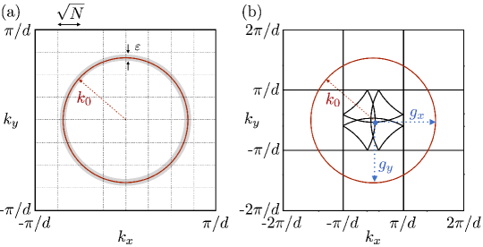
Figure S1: (a) For $d<\lambda_{0}/2$ the light cone (red circle) is contained in the first Brillouin zone, $k_{0}<\pi/d$. The intersection of the $\sqrt{N}\times\sqrt{N}$ black dashed grid lines are the allowed values of $\mathbf{k}$ for a finite $N$ atom array. The gray region around the light cone is excluded to remove the divergence. (b) For $d>\lambda_{0}/2$, the light cone (red circle) is larger than the first Brillouin zone. The black intersecting lines at the center are obtained by folding the light line into the first Brillouin zone. The point $\mathbf{k}$ where two lines intersect (blue circle) can be reached by two distinct scattering processes represented by the vectors $\mathbf{g}_{x,y}$ and satisfying the condition $|\mathbf{k}+\mathbf{g}_{\alpha}|=k_{0}$ for $\alpha=\{x,y\}$ (blue dotted arrows).

Let us now discuss the limit of small and large interatomic separations. Because of the pole in Eqs. (39a,39b), the order of the limits $N\rightarrow\infty$ and $d/\lambda_{0}\rightarrow\infty$ matters. By taking the former first, one recovers the limit of independent atoms $\Gamma_{\text{2D}}^{\parallel,\perp}(\mathbf{k})=\Gamma_{0}$. On the contrary, taking the limit of large separation of Eqs. (39a-39b) does not change the scaling of $\Gamma_{\text{max}}$, as it is fixed by the pole. The limit of vanishing lattice constant follows the same derivation as for 1D arrays, and it is easy to show that, taking the limit $d/\lambda_{0}\rightarrow 0$ before $N\rightarrow\infty$, one recovers Dicke’s scaling $\Gamma_{\mathbf{k}}=N\delta_{\mathbf{k}0}$.

These arguments can be easily generalized to different lattice geometries. The scalings presented above are universal to any 2D array both in the asymptotic limit and for finite $N$, as shown numerically in Fig. 3. Moreover, this figure shows that we numerically recover the analytical limits predicted in this section.

D.3 3D arrays

Infinitely-large 3D arrays do not strictly decay Antezza2009,Brechtelsbauer2021, and the transition rate in momentum space is simply a Dirac delta function at the light cone. Here, we discuss how this divergence is approached as $N$ grows. The maximum transition rate is numerically shown to scale as $\Gamma_{\text{max}}/\Gamma_{0}\sim N^{1/3}$. To prove this result, one can introduce a regularization factor $\Delta\rightarrow 0^{+}$ that controls the divergence of $\Gamma_{\text{3D}}(\mathbf{k})$, and take the limit $N\rightarrow\infty$. One then obtains sierra2022dickeSupp

$$\frac{\Gamma_{\text{3D}}(\mathbf{k})}{\Gamma_{0}}=\frac{6\pi}{k_{0}d^{3}}\sum_{\mathbf{g}}\frac{\Delta(k_{0}^{2}-|(\mathbf{k}+\mathbf{g})\cdot\hat{\bm{\wp}}|^{2})}{(k_{0}^{2}-|(\mathbf{k}+\mathbf{g})|)^{2}+\Delta^{2}k_{0}^{4}},$$ (40)

where $\mathbf{g}=2\pi(n_{x},n_{y},n_{z})/d$ for $n_{x},n_{y},n_{z}\in\mathbb{Z}$ and the sum is extended to all value of $\mathbf{g}$ that satisfy the condition $|\mathbf{k}+\mathbf{g}|<k_{0}$. Following the same reasoning as for 2D arrays, we find $\alpha^{\text{(3D)}}=1/3$ and $\beta^{\text{(3D)}}\sim(k_{0}d)^{-2}$. Similar arguments as for 2D arrays also recover both the Dicke and non-interacting limits.

D.4 Numerical analysis of finite size effects in atomic arrays

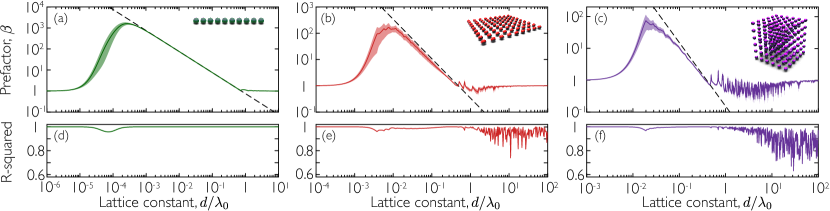
Figure S2: Scaling prefactor (a)-(c) and R-squared value (d)-(f) of the largest transition rate with system size (obtained from a best fit to $\Gamma_{\text{max}}=\beta N^{\alpha}\Gamma_{0}$) as a function of lattice constant for 1D (left panels), 2D (central panels) and 3D (right panels) atomic arrays. The atoms form a square lattice and are polarized parallel to one axis of the array. The fits are done over a region $N_{\text{1D}}\in[2,N^{\text{max}}_{\text{1D}}]$, where $N^{\text{max}}_{\text{1D}}=\{30000,250,40\}$ for 1D, 2D, and 3D, respectively, by sampling seven equally spaced points. The shaded colored area around the lines represents the 1$\sigma$ confidence interval. The dashed lines show the scaling with lattice constant of the prefactor $\beta$ for large arrays. These are $\beta^{(\text{1D})}=3\pi/2k_{0}d$, $\beta^{(\text{2D})}=3\sqrt{\pi}/2(k_{0}d)^{3/2}$, and $\beta^{(\text{3D})}=3/5(k_{0}d)^{2}$, as discussed in Section D.

Figure S2 accompanies Fig. 3 in the main text, and shows the prefactor $\beta$ and R-squared value of the fit to $\Gamma_{\text{max}}=\beta N^{\alpha}\,\Gamma_{0}$ for different array dimensionalities. As discussed in the previous section, the prefactor depends on the lattice constant, and the scaling with $k_{0}d$ agrees with the analytical prediction (shown in dashed lines) over the region where the limit $N\rightarrow\infty$ can be taken regardless of lattice constant. The plots of the R-squared values show that the fit is not good above $d\simeq\lambda_{0}$, where both $\alpha$ and $\beta$ show sharp resonances. These features are a consequence of the crystalline lattice, and can be understood in terms of the addition of previously blocked “umklapp” processes suddenly changing the value of $\Gamma_{\text{max}}$ (see discussion in Section D). These features are generic except for 1D arrays with parallel polarization, as light emission in the direction of the chain is forbidden.

E Exact diagonalization results for 1D and 2D arrays

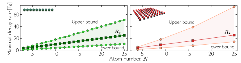
Figure S3: Maximal decay rate $R_{\star}$ obtained from exact diagonalization of $\hat{H}_{\Gamma}$ and upper and lower bounds for 1D (left) and 2D (right) atomic arrays. The lower bound is obtained by numerically evaluating Eq. (5); the upper bound is calculated using Eq. (11). For both plots, atoms are polarized perpendicular to the array and the lattice constant is $d=0.4\lambda_{0}$.

We numerically find the largest eigenvalue of the auxiliary Hamiltonian $\hat{H}_{\Gamma}$ for arrays of up to $N=25$ atoms using the Arpack package in Julia. The results are shown in Fig. S3, together with the upper and lower bounds. To compute the lower bound, we numerically evaluate Eq. (5). For the upper bound, we use Eq. (11). To obtain $\Gamma_{\text{max}}$, we find the maximum eigenvalue by diagonalizing $\mathbf{\Gamma}$, whose elements are given by Eq. (33). We numerically evaluate the spatial variance $\Delta$, using the eigenvector corresponding to $\Gamma_{\text{max}}$.

F Decay rate of typical quantum states

Here, we prove that the decay rate of typical quantum states that are drawn uniformly from the many-body Hilbert space, i.e., via the Haar measure on the unitary group $\mathit{U}(2^{N})$, scales linearly with the system size $N$, implying that typical states do not experience collectively-enhanced decay.

We assume that the Hamiltonian in Eq. (1) contains only geometrically local interactions acting on a constant number of qubits, with non-extensive parameter values. As shown in Section C.2, this only shifts the decay rate $R$ by $O(N)$. Thus, in what follows, we omit the Hamiltonian contribution. The average decay rate (over the Haar measure) is

$$R_{\text{typ}}\equiv\mathbb{E}_{\mathinner{|{\psi}\rangle}\in\text{Haar}}[\mathinner{\langle{\psi|\hat{H}_{\Gamma}|\psi}\rangle}]=\frac{1}{2^{N}}\text{Tr}\hat{H}_{\Gamma}=\frac{1}{2^{N}}\sum_{i,j=1}^{N}\Gamma_{ij}\text{Tr}(\sigma_{i}^{+}\sigma_{j}^{-})=\frac{1}{2^{N}}\sum_{i=1}^{N}\Gamma_{ii}\text{Tr}(\sigma_{i}^{+}\sigma_{i}^{-})=\frac{N\Gamma_{0}}{2},$$ (41)

using $\Gamma_{ii}=\Gamma_{0}$ and $\text{Tr}(\sigma_{i}^{+}\sigma_{i}^{-})=2^{N-1}$ (from the identity acting on the remaining $N-1$ qubits). The value of the typical rate is rather intuitive since the fully excited state $\mathinner{|{e}\rangle}^{\otimes N}$ has a decay rate of $N\Gamma_{0}$, while the ground state $\mathinner{|{g}\rangle}^{\otimes N}$ has a decay rate of $0$. Next, we show that for any typical (Haar random) state, the decay rate is close to $R_{\text{typ}}=N\Gamma_{0}/2$, with a fluctuation that vanishes rapidly with $N$. This arises from the concentration of measure ledoux2001concentration. More precisely, we invoke Levy’s lemma, which in our context states that for any observable $\hat{O}$ and any $\epsilon\geq 0$ mele2024introduction,

$$\text{Pr}\left(\left|\mathinner{\langle{\psi|\hat{O}|\psi}\rangle}-\text{Tr}\hat{O}/2^{N}\right|\geq\epsilon\right)\leq 2\exp\left(-\frac{2^{N}\epsilon^{2}}{18\pi^{3}\|\hat{O}\|^{2}}\right),$$ (42)

where $\mathinner{|{\psi}\rangle}$ is a Haar random state, $\|\hat{O}\|$ is the spectral norm, and Pr stands for probability. In our case, $\hat{O}=\hat{H}_{\Gamma}$, so we have

$$\text{Pr}\left(\left|\mathinner{\langle{\psi|\hat{H}_{\Gamma}|\psi}\rangle}-N\Gamma_{0}/2\right|\geq\epsilon\right)\leq 2\exp\left(-\frac{2^{N}\epsilon^{2}}{18\pi^{3}R_{\star}^{2}}\right).$$ (43)

Since $R_{\star}$ is at most $\sim N^{2}$, the probability of the rate deviating from $R_{\text{typ}}$ is doubly exponentially suppressed in $N$. Thus, the decay rate of a typical state is $N\Gamma_{0}/2$, up to a correction linear in $N$ from the Hamiltonian.

We remark that our conclusion does not only hold for Haar random states, but also more generally for pseudorandom state ensembles known as $k$-designs ambainis2007quantum, which are statistically indistinguishable from the Haar ensemble up to the first $k$ moments. Such states can emerge naturally from the infinite-temperature dynamics of chaotic Hamiltonians, and are also useful for quantum information applications. Perhaps the most well-known example is the set of $N$-qubit stabilizer (Clifford) states, which form a $3$-design webb2016clifford,zhu2017multiqubit. However, for $k$-designs, the concentration result of Eq. (43) does not hold generally. Using large deviation bounds for $k$-designs low2009large, one can show that the probability of the decay rate deviating from $R_{\text{typ}}$ is exponentially suppressed in $N$ (instead of doubly exponentially suppressed).

References

- Haake et al. [1993] F. Haake, M. I. Kolobov, C. Fabre, E. Giacobino, and S. Reynaud, Phys. Rev. Lett. 71, 995 (1993).
- Meiser et al. [2009] D. Meiser, J. Ye, D. R. Carlson, and M. J. Holland, Phys. Rev. Lett. 102, 163601 (2009).
- Bohnet et al. [2012] J. G. Bohnet, Z. Chen, J. M. Weiner, D. Meiser, M. J. Holland, and J. K. Thompson, Nature 484, 78 (2012).
- Narducci et al. [1978] L. M. Narducci, D. H. Feng, R. Gilmore, and G. S. Agarwal, Phys. Rev. A 18, 1571 (1978).
- Carmichael [1980] H. J. Carmichael, J. Phys. B: At. Mol. Opt. Phys 13, 3551 (1980).
- Ferioli et al. [2023] G. Ferioli, A. Glicenstein, I. Ferrier-Barbut, and A. Browaeys, Nat. Phys. 19, 1345 (2023).
- Nielsen and Chuang [2010] M. A. Nielsen and I. L. Chuang, Quantum Computation and Quantum Information: 10th Anniversary Edition (Cambridge University Press, 2010).
- Preskill [2018] J. Preskill, Quantum 2, 79 (2018).
- Lemberger and Yavuz [2017] B. Lemberger and D. D. Yavuz, Phys. Rev. A 96, 062337 (2017).
- González-Tudela et al. [2015] A. González-Tudela, V. Paulisch, D. E. Chang, H. J. Kimble, and J. I. Cirac, Phys. Rev. Lett. 115, 163603 (2015).
- Piñeiro Orioli et al. [2022] A. Piñeiro Orioli, J. K. Thompson, and A. M. Rey, Phys. Rev. X 12, 011054 (2022).
- Mi et al. [2024] X. Mi et al., Science 383, 1332 (2024).
- Leghtas et al. [2015] Z. Leghtas, S. Touzard, I. M. Pop, A. Kou, B. Vlastakis, A. Petrenko, K. M. Sliwa, A. Narla, S. Shankar, M. J. Hatridge, M. Reagor, L. Frunzio, R. J. Schoelkopf, M. Mirrahimi, and M. H. Devoret, Science 347, 853 (2015).
- Gertler et al. [2021] J. M. Gertler, B. Baker, J. Li, S. Shirol, J. Koch, and C. Wang, Nature 590, 243 (2021).
- Kempe et al. [2006] J. Kempe, A. Kitaev, and O. Regev, SIAM J. Comput. 35, 1070 (2006).
- Gharibian et al. [2015] S. Gharibian, Y. Huang, Z. Landau, and S. W. Shin, Found. Trends Theor. Comput. Sci. 10, 159 (2015).
- Osborne [2012] T. J. Osborne, Rep. Prog. Phys. 75, 022001 (2012).
- Bravyi et al. [2019] S. Bravyi, D. Gosset, R. König, and K. Temme, J. Math. Phys. 60, 032203 (2019).
- Endres et al. [2016] M. Endres, H. Bernien, A. Keesling, H. Levine, E. R. Anschuetz, A. Krajenbrink, C. Senko, V. Vuletic, M. Greiner, and M. D. Lukin, Science 354, 1024 (2016).
- Barredo et al. [2016] D. Barredo, S. de Leseleuc, V. Lienhard, T. Lahaye, and A. Browaeys, Science 354, 1021 (2016).
- Kim et al. [2016] H. Kim, W. Lee, H.-g. Lee, H. Jo, Y. Song, and J. Ahn, Nat. Commun. 7, 13317 (2016).
- Kumar et al. [2018] A. Kumar, T.-Y. Wu, F. Giraldo, and D. S. Weiss, Nature 561, 83 (2018).
- Kaufman and Ni [2021] A. M. Kaufman and K.-K. Ni, Nat. Phys. 17, 1324 (2021).
- Bloch et al. [2008] I. Bloch, J. Dalibard, and W. Zwerger, Rev. Mod. Phys. 80, 885 (2008).
- Bluvstein et al. [2024] D. Bluvstein, S. J. Evered, A. A. Geim, S. H. Li, H. Zhou, T. Manovitz, S. Ebadi, M. Cain, M. Kalinowski, D. Hangleiter, J. P. Bonilla Ataides, N. Maskara, I. Cong, X. Gao, P. Sales Rodriguez, T. Karolyshyn, G. Semeghini, M. J. Gullans, M. Greiner, V. Vuletić, and M. D. Lukin, Nature 626, 58 (2024).
- Bakr et al. [2010] W. S. Bakr, A. Peng, M. E. Tai, R. Ma, J. Simon, J. I. Gillen, S. Fölling, L. Pollet, and M. Greiner, Science 329, 547 (2010).
- Bernien et al. [2017] H. Bernien, S. Schwartz, A. Keesling, H. Levine, A. Omran, H. Pichler, S. Choi, A. S. Zibrov, M. Endres, M. Greiner, V. Vuletić, and M. D. Lukin, Nature 551, 579 (2017).
- Scholl et al. [2021] P. Scholl, M. Schuler, H. J. Williams, A. A. Eberharter, D. Barredo, K.-N. Schymik, V. Lienhard, L.-P. Henry, T. C. Lang, T. Lahaye, A. M. Läuchli, and A. Browaeys, Nature 595, 233 (2021).
- Madjarov et al. [2019] I. S. Madjarov, A. Cooper, A. L. Shaw, J. P. Covey, V. Schkolnik, T. H. Yoon, J. R. Williams, and M. Endres, Phys. Rev. X 9, 041052 (2019).
- Norcia et al. [2019] M. A. Norcia, A. W. Young, W. J. Eckner, E. Oelker, J. Ye, and A. M. Kaufman, Science 366, 93 (2019).
- Hutson et al. [2024] R. B. Hutson, W. R. Milner, L. Yan, J. Ye, and C. Sanner, Science 383, 384 (2024).
- Bornet et al. [2023] G. Bornet, G. Emperauger, C. Chen, B. Ye, M. Block, M. Bintz, J. A. Boyd, D. Barredo, T. Comparin, F. Mezzacapo, T. Roscilde, T. Lahaye, N. Y. Yao, and A. Browaeys, Nature 621, 728 (2023).
- Eckner et al. [2023] W. J. Eckner, N. Darkwah Oppong, A. Cao, A. W. Young, W. R. Milner, J. M. Robinson, J. Ye, and A. M. Kaufman, Nature 621, 734a (2023).
- Franke et al. [2023] J. Franke, S. R. Muleady, R. Kaubruegger, F. Kranzl, R. Blatt, A. M. Rey, M. K. Joshi, and C. F. Roos, Nature 621, 740 (2023).
- Mok et al. [2023] W.-K. Mok, A. Asenjo-Garcia, T. C. Sum, and L.-C. Kwek, Phys. Rev. Lett. 130, 213605 (2023).
- Lehmberg [1970] R. H. Lehmberg, Phys. Rev. A 2, 883 (1970).
- Asenjo-Garcia et al. [2017] A. Asenjo-Garcia, M. Moreno-Cardoner, A. Albrecht, H. J. Kimble, and D. E. Chang, Phys. Rev. X 7, 031024 (2017).
- Dicke [1954] R. H. Dicke, Phys. Rev. 93, 99 (1954).
- Gross and Haroche [1982] M. Gross and S. Haroche, Phys. Rep. 93, 301 (1982).
- Marsli [2015] R. Marsli, Int. J. Algebra 9 (2015).
- Lasserre [1995] J. Lasserre, IEEE Trans. Automat. 40, 1500 (1995).
- Wolfe and Yelin [2014] E. Wolfe and S. F. Yelin, Phys. Rev. Lett. 112, 140402 (2014).
- Bojer and von Zanthier [2022] M. Bojer and J. von Zanthier, Phys. Rev. A 106, 053712 (2022).
- Lohof et al. [2023] F. Lohof, D. Schumayer, D. A. W. Hutchinson, and C. Gies, Phys. Rev. Lett. 131, 063601 (2023).
- Renner [2007] R. Renner, Nat. Phys. 3, 645 (2007).
- Caves et al. [2002] C. M. Caves, C. A. Fuchs, and R. Schack, J. Math. Phys. 43, 4537 (2002).
- Sierra et al. [2022] E. Sierra, S. J. Masson, and A. Asenjo-Garcia, Phys. Rev. Res. 4, 023207 (2022).
- Boyd and Vandenberghe [2004] S. Boyd and L. Vandenberghe, Convex Optimization (Cambridge University Press, 2004).
- Barthel and Hübener [2012] T. Barthel and R. Hübener, Phys. Rev. Lett. 108, 200404 (2012).
- Baumgratz and Plenio [2012] T. Baumgratz and M. B. Plenio, New J. Phys. 14, 023027 (2012).
- Baccari et al. [2020] F. Baccari, C. Gogolin, P. Wittek, and A. Acín, Phys. Rev. Res. 2, 043163 (2020).
- Parekh and Thompson [2021] O. Parekh and K. Thompson, in 48th International Colloquium on Automata, Languages, and Programming (ICALP 2021), Leibniz International Proceedings in Informatics (LIPIcs), Vol. 198 (Schloss Dagstuhl – Leibniz-Zentrum für Informatik, Dagstuhl, Germany, 2021) pp. 102:1–102:20.
- Wang et al. [2024] J. Wang, J. Surace, I. Frérot, B. Legat, M.-O. Renou, V. Magron, and A. Acín 10.48550/arXiv.2310.05844 (2024), arXiv:2310.05844 [quant-ph] .
- Diamond and Boyd [2016] S. Diamond and S. Boyd, J. Mach. Learn. Res. 17, 1 (2016).
- Masson and Asenjo-Garcia [2022] S. J. Masson and A. Asenjo-Garcia, Nat. Commun. 13, 2285 (2022).
- Rubies-Bigorda et al. [2023] O. Rubies-Bigorda, S. Ostermann, and S. F. Yelin, Phys. Rev. Res. 5, 013091 (2023).
- Masson et al. [2020] S. J. Masson, I. Ferrier-Barbut, L. A. Orozco, A. Browaeys, and A. Asenjo-Garcia, Phys. Rev. Lett. 125, 263601 (2020).
- Block et al. [2023] M. Block, B. Ye, B. Roberts, S. Chern, W. Wu, Z. Wang, L. Pollet, E. J. Davis, B. I. Halperin, and N. Y. Yao 10.48550/arXiv.2301.09636 (2023), arXiv:2301.09636 .
- Mitchell and Palacios Alvarez [2020] M. W. Mitchell and S. Palacios Alvarez, Rev. Mod. Phys. 92, 021001 (2020).
- Aharonov et al. [2006] D. Aharonov, A. Kitaev, and J. Preskill, Phys. Rev. Lett. 96, 050504 (2006).
- Preskill [2013] J. Preskill, Quantum Info. Comput. 13, 181 (2013).
- Cong et al. [2022] I. Cong, H. Levine, A. Keesling, D. Bluvstein, S.-T. Wang, and M. D. Lukin, Phys. Rev. X 12, 021049 (2022).
- Manetsch et al. [2024] H. J. Manetsch, G. Nomura, E. Bataille, K. H. Leung, X. Lv, and M. Endres 10.48550/arXiv.2403.12021 (2024), arXiv:2403.12021 [quant-ph] .
- Campaioli et al. [2023] F. Campaioli, S. Gherardini, J. Q. Quach, M. Polini, and G. M. Andolina 10.48550/arXiv.2308.02277 (2023), arXiv:2308.02277 [quant-ph] .
- Scholes et al. [2011] G. D. Scholes, G. R. Fleming, A. Olaya-Castro, and R. van Grondelle, Nat. Chem. 3, 763 (2011).

References

- Horn and Johnson [2012] R. A. Horn and C. R. Johnson, Matrix Analysis, 2nd ed. (Cambridge University Press, 2012).
- Carmichael [1993] H. J. Carmichael, An open systems approach to quantum optics (Springer-Verlag, Berlin Heidelberg, 1993).
- Lehmberg [1970] R. H. Lehmberg, Phys. Rev. A 2, 883 (1970).
- Asenjo-Garcia et al. [2017] A. Asenjo-Garcia, M. Moreno-Cardoner, A. Albrecht, H. J. Kimble, and D. E. Chang, Phys. Rev. X 7, 031024 (2017).
- Jackson [1999] J. D. Jackson, Classical electrodynamics, 3rd ed. (Wiley, New York, NY, 1999).
- Antezza and Castin [2009] M. Antezza and Y. Castin, Phys. Rev. Lett. 103, 123903 (2009).
- Brechtelsbauer and Malz [2021] K. Brechtelsbauer and D. Malz, Phys. Rev. A 104, 013701 (2021).
- Sierra et al. [2022] E. Sierra, S. J. Masson, and A. Asenjo-Garcia, Phys. Rev. Res. 4, 023207 (2022).
- Ledoux [2001] M. Ledoux, The Concentration of Measure Phenomenon (American Mathematical Society, 2001).
- Mele [2024] A. A. Mele, Quantum 8, 1340 (2024).
- Ambainis and Emerson [2007] A. Ambainis and J. Emerson, in Twenty-Second Annual IEEE Conference on Computational Complexity (CCC’07) (2007) pp. 129–140.
- Webb [2016] Z. Webb, Quantum Inf. Comput. 16, 1379 (2016).
- Zhu [2017] H. Zhu, Phys. Rev. A 96, 062336 (2017).
- Low [2009] R. A. Low, Proc. Math. Phys. Eng. Sci. 465, 3289 (2009).