Age-Gain-Dependent Random Access for Event-Driven Periodic Updating
Abstract
This paper considers utilizing the knowledge of age gains to reduce the average age of information (AoI) in random access with event-driven periodic updating for the first time. Built on the form of slotted ALOHA, we require each device to determine its age gain threshold and transmission probability in an easily implementable decentralized manner, so that the contention can be limited to devices with age gains as high as possible. For the basic case that each device utilizes its knowledge of age gain of only itself, we provide an analytical modeling by a multi-layer discrete-time Markov chains (DTMCs), where an external DTMC manages the jumps between the beginnings of frames and an internal DTMC manages the evolution during an arbitrary frame, for obtaining optimal access parameters offline. For the enhanced case that each device utilizes its knowledge of age gains of all the devices, we require each device to adjust its access parameters for maximizing the estimated network expected AoI reduction per slot, through maintaining a posteriori joint probability distribution of local age and age gain of an arbitrary device in a Bayesian manner. Numerical results validate our study and demonstrate the advantage of the proposed schemes over other schemes.
Index Terms:
Internet of Things, age of information, periodic update, random access, slotted ALOHA.I Introduction
I-A Background
Internet of Things (IoT) systems have been widely applied in many real-time services [1, 2, 3], such as emergency surveillance, target tracking, process control, and so on. In these services, destinations are interested in the status of one or multiple processes observed by multiple sources, and then take necessary actions based on the received status updates. To ensure the quality and even safety of these services, it is typically necessary for sources to deliver their generated updates to the corresponding destinations as timely as possible.
However, such timeliness requirement cannot be characterized adequately by conventional performance metrics (e.g. throughput and delay). For example, when the throughput is large, the received updates may not be fresh due to long delay; when the delay is small, the received updates may not be fresh due to infrequent arrivals of updates. As such, a new performance metric, termed age of information (AoI), has been introduced in [4] to measure the time elapsed since the generation moment of the latest successfully received update at a destination. Naturally, to reduce the network average AoI (AAoI), it is desirable for multiple access schemes to assign higher transmission priorities to devices with higher age gains, where the age gain of a device in a slot quantifies how much a successful transmission of this device will reduce its corresponding instantaneous AoI. Note that the age gain of a device depends on only its instantaneous AoI under the generate-at-will (GAW) arrival of updates.
With this objective, scheduling schemes that operate in a centralized manner without contentions have been designed to perform close to optimal network AAoI in various scenarios [5, 6, 7, 8]. However, they may be impractical to implement due to the huge overhead of required coordination, especially when there is considerable uncertainty on the arrival patterns of updates. Unlike scheduling schemes, random access schemes (e.g. slotted ALOHA, frame slotted ALOHA, CSMA) allow a population of devices with limited or no coordination to dynamically and opportunistically share a channel. So, it is strongly required to design age-gain-dependent random access (AGDRA) schemes, where each device utilizes its knowledge of age gains to determine when to transmit its updates in an easily implementable decentralized manner, so that the unavoided contention can be limited to devices with age gains as high as possible.
Various AGDRA schemes have been proposed for the GAW arrival [9, 10, 11, 12, 13, 14, 15, 16] and the Bernoulli arrival [17, 18, 19, 20] of updates, and have been shown to significantly reduce the network AAoI compared to conventional random access schemes. It can be observed from [16, 17, 9, 10, 11, 12, 13, 14, 15, 20, 18, 19] that designing AGDRA is uniquely challenging due to the inherent coupling of the arrival process of updates, the time evolution of local ages, the time evolution of AoIs, and the time-varying mutual interference. Generally speaking, this coupling would become more complicated when a more general arrival process of updates is considered, and is quite different from that for optimizing the throughput or delay metric.
I-B Related Work
Without relying on the knowledge of age gains, many conventional random access schemes have been proposed for minimizing the network AAoI. Under the GAW arrival, [21] showed that using slotted ALOHA is worse than scheduling by a factor of about . Under the Bernoulli arrival, [22] used the elementary renewal theorem to optimize the transmission probabilities for slotted ALOHA and CSMA, while [23] used discrete-time Markov chains (DTMCs) to optimize the frame length for frame slotted ALOHA. Under the periodic arrival, [24] analyzed the effect of maximizing the instantaneous throughput on the network AAoI of slotted ALOHA.
Basic AGDRA, where each device utilizes its knowledge of age gain of only itself to adjust its access parameters, has been investigated in [17, 20, 9, 10, 11, 14, 15, 12, 13]. In the form of slotted ALOHA, [9, 10, 11, 14, 15, 12, 13] assumed that each device adopts a fixed transmission probability if its corresponding age gain reaches a fixed threshold, but keeps silent otherwise. Based on a comprehensive steady-state analysis of the DTMC defined in [9], closed-form expressions of the network AAoI and optimal access parameters were provided in [10] for an infinitely large network size. For an arbitrary network size, [11] analyzed the network AAoI by modeling the AoI evolution of each device as a DTMC, which, however, relies on an ideal assumption that the states of all the devices are independent of each other. To mitigate the negative impact of contentions, a reservation phase ahead of actual data transmission is proposed in [12, 13], but its benefit comes at a cost of additional overhead compared to [9, 11, 10]. Further, [15, 14] used stochastic geometry tools to derive the network AAoI under the spatiotemporal interference. Note that [9, 11, 10, 14, 15, 12, 13] mainly focused on the GAW traffic, except that [10] extended its findings to obtain an upper bound on the network AAoI for the Bernoulli arrival. These schemes [9, 10, 11, 14, 15, 12, 13] have a common advantage that the access parameters can be obtained offline through analytical modeling, and thus can be simply implemented. In addition, heuristic methods proposed in [17, 20] allow each device to use different transmission probabilities for different cases, but lack analytical modeling.
To further reduce the network AAoI, enhanced AGDRA, where each device utilizes its knowledge of age gains of all the devices to adjust its access parameters, has been investigated in [18, 19] for the Bernoulli arrival. In the form of slotted ALOHA, the AAT proposed in [18] allows each device to transmit with a dynamic transmission probability (determined by the estimated number of active devices) for maximizing the instantaneous network throughput only if its corresponding age gain reaches a threshold, which could be computed adaptively using the estimated distribution of age gains. In the form of frame slotted ALOHA, the practical T-DFSA proposed in [19] allows the frame length and age-gain threshold for each frame to be adjusted by the estimated distribution of age gains, so that the estimated expected number of active devices can be the smallest number not smaller than a certain number (searched by simulations). Different from [18, 19], under the GAW arrival, [16] estimated the network AoI rather than the individual age gains for heuristically adjusting the transmission probability, which would obviously lead to the AoI degradation.
However, these previous studies on AGDRA [17, 9, 10, 11, 12, 13, 14, 15, 18, 19, 16, 20] have not considered the event-driven periodic arrival of updates, which usually appears in many monitoring services[25, 26, 27, 28]. For example, in closed-loop process control, multiple sensors are employed to measure the plant outputs and validate the event conditions periodically, and then each sensor sends a fresh status update to a machine controller as needed. Note that such an arrival process can include those considered in[17, 9, 10, 11, 12, 13, 14, 15, 18, 19, 20, 24, 21, 22, 23, 16] as particular cases.
I-C Contributions
To fill the gap in this field, this paper attempts to design a type of AGDRA in the form of slotted ALOHA with an age gain threshold [9, 10, 11, 14, 15, 12, 13, 18, 19], called T-AGDSA, under event-driven periodic updating. Compared to the existing work [24, 11, 10, 18, 19], this paper makes the following key contributions.
-
1.
Basic T-AGDSA: For simple implementation, consider fixed threshold and fixed transmission probability as in [9, 10, 11, 14, 15, 12, 13]. We provide an analytical modeling approach to evaluate the network AAoI under event-driven periodic updating, based on which optimal threshold and optimal transmission probability can be obtained offline. Compared to [24, 11, 10], the technical difficulty of our work is to consider the mutual impact of event-driven periodic updating and the age-gain-dependent behavior in modeling, which is overcome by a multi-layer DTMC model. Here an external DTMC manages the jumps between the beginnings of frames, while an internal DTMC manages the evolution during an arbitrary frame. Note that the modeling approaches in [24, 11] can be seen as special cases here.
-
2.
Enhanced T-AGDSA: To pursue lower network AAoI, we propose an enhanced T-AGDSA scheme that allows each device to adjust the threshold and the transmission probability for maximizing the estimated network expected AoI reduction (EAR) per slot, based on the knowledge of age gains of all the devices. Such knowledge comes from using Bayes’ rule to keep a posteriori joint probability distribution of local age and age gain of an arbitrary device. Compared with the AAT [18] that maximizes the estimated instantaneous network throughput under a reasonably controlled effective sum arrival rate, our scheme can avoid low efficiency of the throughput-EAR conversion. Compared with the practical T-DFSA [19] that controls the estimated expected number of active devices reasonably, our scheme can avoid the network EAR degradation when the probability distribution of the estimated number is divergent.
Through extensive numerical experiments, we validate our theoretical analysis and demonstrate the advantage of the proposed schemes over the schemes in [24, 10, 18, 19] in a wide range of network configurations.
The remainder of this paper is organized as follows. The system model, the considered two versions of T-AGDSA, and a lower bound on the network AAoI are specified in Section II. In Section III, we provide an analytical modeling approach to evaluate basic T-AGDSA for determining optimal fixed access parameters. In Section IV, we propose an enhanced T-AGDSA scheme for maximizing the estimated network EAR per slot. Section V provides numerical results to verify our study. Section VI draws final conclusions.
II System Model and Preliminaries
II-A Network Model
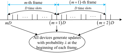
Consider a globally-synchronized uplink IoT system consisting of a common access point (AP) and devices, indexed by . As shown in Fig. 1, the global channel time is divided into frames (indexed from frame 0), each of which consists of consecutive slots. The slots in frame are indexed from slot to . At the beginning of each frame, each device independently generates a single-slot update with probability and does not generate updates at other time points. To maintain the information freshness, a newly generated update at each device will replace the undelivered older one if there is any.
By considering a reliable wireless channel under an appropriate modulation and coding scheme, we assume that an update is successfully transmitted if it is not involved in a collision, and otherwise is unsuccessfully transmitted. After a successful reception of an update of a device, the AP immediately sends an acknowledgment (ACK) to notify the device without errors or delays. Thus, at the end of each slot , each device is able to be aware of the channel status of slot , denoted by .
II-B Performance Metrics
At the beginning of slot , we denote the local age of device by , which measures the number of slots elapsed since the generation moment of its freshest update. The local age of device is reset to zero if the device generates a new update at the beginning of slot , otherwise, it increases by one. Then, the evolution of with is given by
| (1) |
Next, we denote the instantaneous AoI of device at the beginning of slot by , which measures the number of slots elapsed since the generation moment of its most recently successfully transmitted update. If the freshest update of device is transmitted successfully at slot , the AoI of device will be set to its local age (in the previous time slot) plus one, otherwise, the AoI will increase by one. Then, the evolution of with is given by
| (2) |
Owing to the ACK mechanism and local information about , each device is able to be aware of the value of at the beginning of slot for each .
We define the AAoI of device as:
| (3) |
This paper aims to design a decentralized access protocol that minimizes the network AAoI,
| (4) |
II-C Random Access Protocol
We define the age gain of device at the beginning of slot as
| (5) |
which quantifies the reduction in instantaneous AoI upon a successful transmission of device . Based on the fact that , it is clear that .
Following [18], we require each device with a non-empty buffer (i.e., ) to send its update according to the following T-AGDSA protocol, that is,
-
1.
transmits at the beginning of slot with the probability if where the threshold can be an arbitrary positive integer,
-
2.
otherwise keeps silent at slot .
A device is said to be active in slot if .
Then, we consider the following two versions of T-AGDSA with different settings of and :
-
1.
Basic T-AGDSA: for simple implementation [10], the values of and are fixed to and , respectively, for all slots .
-
2.
Enhanced T-AGDSA: at the beginning of each slot , each device determines the values of and based on the knowledge of age gains of all the devices. Such knowledge comes from the globally available information, including the network parameters , , , previous channel status , and previous access parameters , . Note that, since the devices only use global information to compute and , each device will obtain the same values of them.
It will be shown in Sections III–V that basic T-AGDSA can be designed offline through theoretical modeling and is simpler to implement compared to enhanced T-AGDSA, but cannot utilize the knowledge of age gains of all the devices to improve the AoI performance as done in enhanced T-AGDSA.
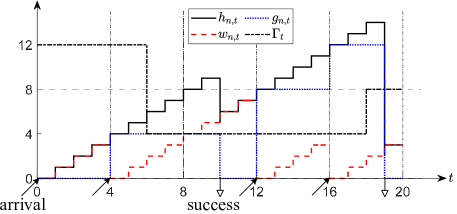
An example of , , and evolving over time under enhanced T-AGDSA when is shown in Fig. 2.
II-D Lower bound
When , [18] derived a lower bound on the achievable network AAoI by assuming that all updates can be delivered instantaneously upon their arrival, without experiencing collisions. We extend this bound to the case . This bound is tighter when is smaller, which will be verified in Section V. The proof is given in Appendix.
Proposition 1: For any transmission scheme under the system model specified in Section II-A,
| (6) |
III Modeling and Design of Basic T-AGDSA
In this section, we provide an analytical modeling approach to evaluate the network AAoI of basic T-AGDSA, and use this modeling to obtain optimal values of fixed threshold and fixed transmission probability .
The symmetric scenario described in Section II allows us to analyze the AAoI of an arbitrarily tagged device to represent the network AAoI. So, we omit the device index for analysis simplicity. To reflect the impact of the frame length better, we identify a slot by the tuple , where and , for arbitrary . The main notations used in our analysis are listed in Table I.
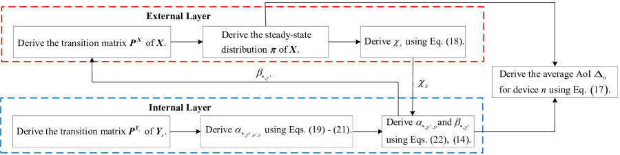
To calculate the AAoI of the tagged device, as shown in Fig. 3, we adopt a multi-layer Markov model where the external layer manages the jumps between the beginnings of frames, while the internal layer manages the evolution during an arbitrary frame. In the rest of this section, we explore how to establish these two coupled layers.
| Notation | Description |
| The instantaneous AoI, local age, and age gain of the tagged device at the beginning of frame . | |
| An external DTMC with the infinite state space . | |
| The transition matrix of . | |
| The probability that the tagged device transmits its -th update successfully in slot given . | |
| The probability that the tagged device transmits its -th update successfully in frame given . | |
| for and . | |
| for and . | |
| The steady-state probability of staying at state for . | |
| The number of active devices not including the tagged device at the beginning of an arbitrary frame . | |
| The probability mass function of . | |
| An absorbing DTMC with the finite state space . | |
| State indicating the transmission results of all devices before the beginning of slot . | |
| The transition matrix of . | |
| The probability that the tagged device transmits its -th update successfully at slot when , . |
III-A External Layer
Let and denote the local age and instantaneous AoI of the tagged device at the beginning of frame , respectively. By Eq. (1) and the traffic pattern described in Section II, the evolution of with can be expressed as
| (7) |
By Eq. (2), the evolution of with can be expressed as
| (8) |
Denote the age gain of the tagged device at the beginning of frame by . By Eq. (5), we have
| (9) |
Consider a state process where . By Eqs. (7)–(9), we observe that the transition to the next state in depends only on the present state and not on the previous states. Hence, can be viewed as a DTMC with the infinite state space .
For an arbitrary frame with , let and denote the probabilities that the tagged device transmits its update successfully at slot and in frame , respectively. Obviously, . According to the evolution of and given in Eqs. (7)–(9), the state transition probabilities of can be obtained as
| (10) |
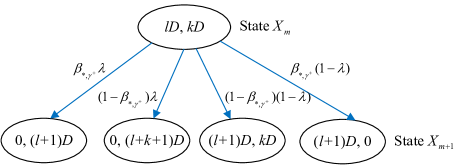
Consider that under the traffic pattern described in Section II, the age gain of the tagged device during frame remains unchanged if the tagged device fails to transmit its update successfully in frame ; otherwise, the age gain will reduce to zero and remain zero in the subsequent slots during frame after a successful transmission. Thus, the age gain of the tagged device in each slot takes value from . This observation allows us to set , and discuss possible values of and in Eq. (10) based on different values of , , and .
Case 1: When , we have . Consider that the tagged device keeps its age gain unchanged during frame if it does not make a successful transmission during frame . So, the tagged device always keeps silent in frame as its age gain is always smaller than . Then we obtain
| (11) | ||||
| (12) |
if and . With Eqs. (10)–(12), the state transitions for this case are illustrated in Fig. 4(a).
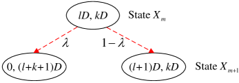
Case 2: When , we have , the tagged device transmits its update with a fixed probability at the beginning of slot when until a successful transmission. Note that the tagged device behaves the same during frame regardless of the values of , when . So, we rewrite and simply as
| (13) | ||||
| (14) |
if and . Note that and are independent of values of and . With Eqs. (10), (13), and (14), the state transitions for this case is illustrated in Fig. 4(b).
Note that the state in is an ephemeral state only occurring when (i.e., ), while the remaining states are all in the same recurrent class and occur when (i.e., ). As increases, will get absorbed in the recurrent class, and it will stay there forever. Denote by the steady-state distribution of . Each element denotes the steady-state probability of staying at state . We assume that .
Then, for different states in , we consider the following two cases for evaluating the AAoI of the tagged device during an arbitrary frame with .
Case 1: The tagged device transmits its update successfully at slot given . Let denote the AAoI of the tagged device during frame when this event occurs. We have
| (15) |
Case 2: The tagged device fails to transmit its update successfully during frame given . Let denote the AAoI of the tagged device during frame when this event occurs. We have
| (16) |
III-B Internal Layer to Evaluate
Note that whether the tagged device can transmit its update successfully depends on the behaviors of all active devices during frame . Let a random variable denote the number of active devices not including the tagged device at the beginning of an arbitrary frame , and let denote the probability mass function of . Following [11], we make a simplifying decoupling assumption that the states of all the devices are independent of each other. Then, based on the binomial distribution, we have
| (18) |
for each .
Consider an arbitrary frame with and . Define as an absorbing DTMC with the finite state space , as shown in Fig. 5. The states with are transient states indicating that, during frame , the tagged device has not transmitted successfully before the beginning of slot while other devices have transmitted successfully before the beginning of slot . The state is an absorbing state indicating that, during frame , the tagged device has transmitted successfully before the beginning of slot . For convenience, the slot index is used to denote the slot index here. As shown in Fig. 5, the state transition probabilities of can be obtained as
| (19) |
The first case in Eq. (III-B) corresponds to that no device makes a successful transmission in slot when . The second case corresponds to that one of the other devices makes a successful transmission in slot when . The third case corresponds to that the tagged device makes a successful transmission in slot when . The fourth case corresponds to that the tagged device has made a successful transmission before the beginning of slot .
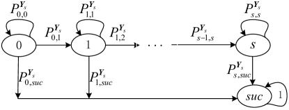
Let denote the state vector of , where the -th element corresponds to the state for and the last element corresponds to the state . Then, given the priori state vector and the transition matrix based on Eq. (III-B), by applying a simple power method, we have
| (20) |
for each and .
III-C Evaluation of
Now we are ready to use the following three steps to compute by connecting the external and internal layers proposed in previous subsections.
Step 1: Based on the transition probabilities in Eq. (10), the steady-state distribution can be obtained by solving a set of linear equations
| (23) |
and the normalizing condition
| (24) |
Since is involved as the only unknown parameter in the transition matrix , each can be expressed as a function of using a mathematical induction method based on Eqs. (10), (23), (24). Meanwhile, in Eq. (14) can be expressed as a function of based on Eqs. (18)–(22). Hence, we can obtain the value of by solving Eq. (14) using numerical methods like the fixed-point iteration method.
Step 2: With the value of , we can obtain the values of by Eqs. (10), (23) and (24), and then obtain the values of by Eqs. (18)–(22).
Step 3: With the values of , and , we can obtain the AAoI for an arbitrary device by Eq. (17).
Remark 1: When , we note that we can drop the subscripts of and have for since is independent of and . So, our modeling approach is reduced to that in [24].
Remark 2: When (i.e., the GAW traffic), we have , for each , and
| (25) |
So, our modeling approach is reduced to that in [11].
Remark 3: In general, there may exist multiple solutions of in step 1 since Eq. (18) assumes that the states of all the devices are independent of each other, which requires simulations to help us identify the correct solution. When , [10] presented a precise steady-state analysis without this ideal assumption. A key idea therein is to utilize an inherent feature for , that is, different inactive devices have different age gains. However, it is inapplicable for or because there may exist multiple inactive devices with the same age gain.
III-D Seeking Optimal and
In order to seek optimal values of and , we can view given in Eq. (17) as a function of both and , denoted by . However, it is difficult to obtain the gradient of due to the lack of an explicit expression. So, well-known two-dimensional gradient-free search methods, such as the Hooke-Jeeves method, and Rosenbrock method, can be applied. Moreover, since the age gain of each device is always an integral multiple of as described in Section III-A, we can consider only to reduce the search space.
IV Design of Enhanced T-AGDSA
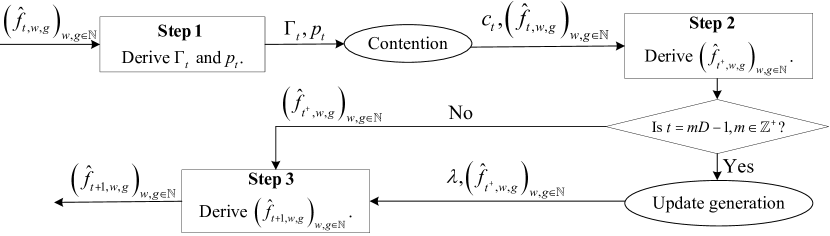
In this section, we propose an enhanced T-AGDSA scheme that allows each device to adjust the threshold and the transmission probability for maximizing the estimated network EAR per slot, based on the knowledge of age gains of all the devices. After introducing the basic idea of our design, we will present a comprehensive explanation of the three key steps as shown in Fig. 6.
IV-A Basic Idea
Define the AoI reduction of device in slot as
| (26) |
We can use Eqs. (2), (5) and (26) to compute as follows.
| (27) |
Let denote the success probability when device transmits in slot . From Eq. (27), we can obtain the EAR of device in slot as
| (28) |
where is the indicator function of event and denotes the number of active devices not including device in slot . Then, the network EAR in slot can be obtained as
| (29) |
This section will investigate how each device uses globally available information to choose and for maximizing . Note that, although it may be possible to achieve better results by using information local to the devices, or using a strategy to maximize the long-run network EAR that is not “one-step look-ahead”, we do not pursue these possibilities here.
From Eqs. (IV-A) and (29), it is easy to see that the knowledge of the age gains , is essential for maximizing . However, in practice, it is impossible for each device to obtain precise values of the age gains of other devices. So, we require each device to keep a posteriori joint probability distribution of local age and age gain of an arbitrarily tagged device at the beginning of slot , given all of the globally available information. We denote such a distribution by , where . Based on , a brief introduction of the three key steps of the proposed enhanced T-AGDSA as shown in Fig. 6 is given below:
Step 1: At the beginning of slot , each device uses to obtain an estimate of network EAR, denoted by , and then chooses and that maximize .
Step 2: At the end of slot , each device uses the observed channel status to update in a Bayesian manner. We denote the resulting distribution in this step by , where represents the end of slot .
Step 3: At the beginning of slot , if , each device obtains using and the update generation probability , otherwise, each device obtains .
Remark 4: In AAT [18], is chosen so that the effective sum arrival rate approaches as close as possible and is then chosen for maximizing the instantaneous network throughput. However, such a setting may yield unsatisfactory network EAR, since it allows the devices with low age gains to compete for the transmission opportunity as soon as the effective sum arrival rate does not exceed . In other words, in a slot, higher network throughput cannot be certainly converted to larger network EAR.
Remark 5: In practical T-DFSA [19], the maximum value of the thresholds that make the estimated expected number of active devices not smaller than a certain number (searched by simulations) is chosen. However, such a setting may yield unsatisfactory network EAR, since its design objective may be far from maximizing the network EAR, especially when the probability distribution of the estimated number of active devices is divergent.
Remark 6: Both AAT [18] and practical T-DFSA [19] ideally assume that the age gain and local age of a device are independent of each other, thus only consider the distribution of age gain. However, there is a strong dependency between them as described in Eq. (5). This is indeed why we consider .
Remark 7: The AAT [18] utilizes only the collision feedback to update its estimate, while our enhanced T-AGDSA scheme utilizes the ternary feedback (idle, success, collision). Nevertheless, our scheme requires no additional overhead owing to the ACK mechanism.
IV-B Choosing and based on
In the following, we present how to estimate the network EAR in slot based on by assuming that the states of all the devices are independent of each other.
Let denote the estimated number of active devices not including an arbitrary device in slot . Based on the binomial distribution, we have
| (30) |
for each , where
| (31) |
denotes the probability of an arbitrary device being active in slot .
From Eq. (30), we obtain the estimated success probability of an arbitrary transmission in slot as follows.
| (32) |
From Eqs. (27) and (32), we can obtain the following estimate of network EAR in slot .
| (33) |
We can view as a function of and , denoted by . We see from Eq. (33) that, for each given , the maximization of is equivalent to the maximization of . So we can obtain the value that maximizes by differentiating and root finding since is a polynomial of . However, in practice, such computation would probably be excessive. Following [29, 30], we can approximate as follows.
| (34) |
Since the function is unimodal in our implementation, we can obtain the value that maximizes through an efficient one-dimensional search method. Moreover, due to the same argument in Section III-D, we can consider only to reduce the search space.
IV-C Computing Using Channel Observations
Let and denote the local age and age gain of an arbitrary device at the end of slot , respectively. Given all globally available information at the end of slot , each device is able to compute using Bayes’ rule as follows.
| (35) |
for each , where
| (36) |
and
| (37) |
In Eq. (IV-C), the first and second cases correspond to that no devices transmits, the third and fourth cases correspond to that one of the other devices transmits successfully, the fifth case corresponds to that the tagged device transmits successfully when it is active in slot , the sixth and seventh cases correspond to that a collision occurs.
IV-D Computing Using the Update Generation Probability
It remains to obtain at the beginning of slot based on and the update generation probability .
Initially, for each , each device knows
| (38) |
which implies
| (39) |
Considering that each device independently generates an update with probability at the beginning of each frame (i.e., ) and does not generate updates at other time points, we have
| (40) |
for each , where
| (41) |
The proposed enhanced T-AGDSA is summarized in Algorithm 1.
V Numerical Results
This section consists of three subsections. The first subsection validates the analytical modeling of the proposed basic T-AGDSA and examines its advantage over the schemes in [24, 10, 22, 21]. The second subsection examines the advantage of the proposed enhanced T-AGDSA over the schemes in [24, 18, 19]. The third subsection compares the proposed basic T-AGDSA and enhanced T-AGDSA. The scenarios considered in the simulations are in accordance with the descriptions in Section II. We shall vary the network configuration over a wide range to validate our theoretical study. Each simulation result is obtained from 10 independent simulation runs with slots in each run.
V-A Proposed Basic T-AGDSA
We consider the following two simply implemented schemes as benchmarks.
- 1.
-
2.
Threshold-ALOHA for [10]: each device uses an optimal fixed and an optimal fixed when , and uses an suboptimal fixed and an suboptimal fixed when , .
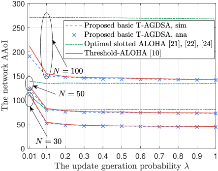
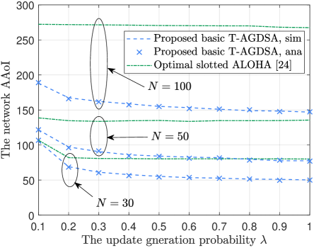
Fig. 7(a) shows the network AAoI of the proposed basic T-AGDSA as a function of the update generation probability for different when . The curves indicate that our analytical modeling is accurate in all the cases. We observe that the network AAoI of all the three schemes first decreases with and then remains almost the same. This is because larger is helpful to reduce the AAoI due to the delivery of fresher updates, but this effect would become weaker due to severer contention when is larger. We also observe that the proposed basic T-AGDSA enjoys up to improvement over the optimal slotted ALOHA [24, 21, 22], which verifies the benefit of introducing the fixed threshold . We further observe that the proposed basic T-AGDSA enjoys up to improvement over the threshold-ALOHA [10] in large-scale networks with sporadic individual traffic (i.e., when is large and is small), but performs almost the same in other cases. This is because the age gain threshold is more helpful in reducing the AAoI compared with the AoI threshold used in the threshold-ALOHA [10] and this advantage is notable when is large and is small. Meanwhile, this advantage is enlarged when is small because the threshold-ALOHA [10] used the assumption of to obtain the transmission policy when .
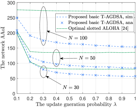
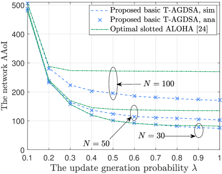
Fig. 7(b)–(d) show the network AAoI of the proposed basic T-AGDSA as a function of for different when , respectively. Note that the threshold-ALOHA [10] is inapplicable when . The accuracy of our analytical modeling is verified again in these cases. We observe that, compared with optimal slotted ALOHA [24], the proposed basic T-AGDSA enjoys up to improvement when , up to improvement when , and up to improvement when . These results indicate that introducing is effective in improving the AAoI for a wide range of configurations. We further observe that, in general, the advantage of the proposed basic T-AGDSA diminishes when decreases, decreases, or increases. This is because the effect of introducing to mitigate the contention becomes weaker in these cases.
V-B Proposed Enhanced T-AGDSA
We consider the following four ideal or high-computational-overhead schemes as benchmarks.
-
1.
Ideal scheduling [18]: the AP always selects one of the devices with the highest age gains to transmit. Obviously, it provides a lower bound on the network AAoI.
-
2.
Ideal adaptive slotted ALOHA [24]: each device uses and , where represents the number of active devices in slot .
- 3.
- 4.
In addition, we consider another lower bound for stated in Proposition 1 by assuming no collisions.
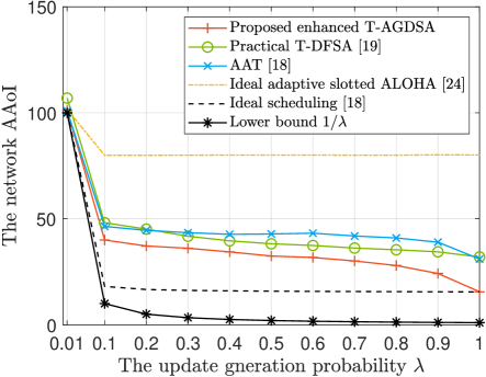
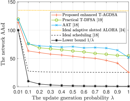
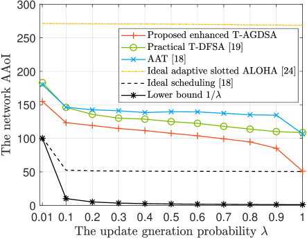
Fig. 8 shows the network AAoI of the proposed enhanced T-AGDSA as a function of for different when . We observe that the network AAoI of the ideal adaptive slotted ALOHA [24] first decreases with and then remains almost the same, while that of the other three schemes always decreases with due to the effect of introducing the adaptive threshold. We also observe that the enhanced T-AGDSA enjoys up to improvement over the ideal adaptive slotted ALOHA [24]. This verifies the benefit of introducing the adaptive threshold , even if the latter utilizes the ideal knowledge of . We further observe that the enhanced T-AGDSA enjoys up to improvement over the AAT [18], and enjoys up to improvement over the practical T-DFSA [19]. This is owing to our more reasonable , which is computed by not only a more accurate estimation of the age gains (see Remark 6) but also a more reasonable optimization goal (see Remarks 4 and 5). We also observe that all the schemes enjoy almost the same AAoI (close to ) when is small, which confirms the lower bound proposed in [18]. This is because the inter-arrival time becomes a dominant factor to determine the AAoI when the network traffic is quite low. On the other hand, when is not small, we note that the enhanced T-AGDSA performs closer to the ideal scheduling [18] as increases, which implies that our adaptive threshold can be chosen to limit the contention to fewer devices with higher age gains due to a more accurate estimation of age gains.
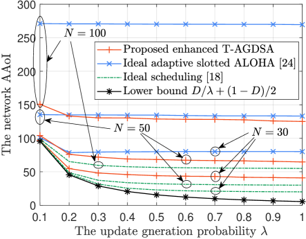
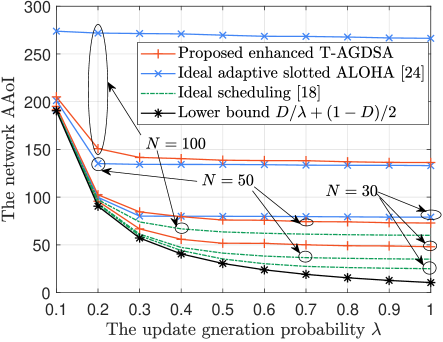
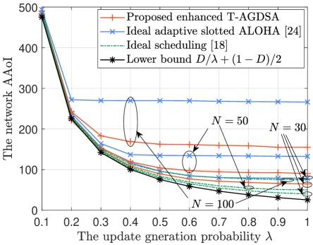
Fig. 9 shows the network AAoI of the proposed enhanced T-AGDSA as a function for different when . Note that the AAT [18] and the practical T-DFSA [19] are both inapplicable when . We observe that, compared with the ideal adaptive slotted ALOHA [24], the enhanced T-AGDSA enjoys up to improvement when , up to improvement when , and up to improvement when . These results indicate that introducing the adaptive is effective in improving the AAoI for a wide range of configurations. We further observe that such improvement diminishes when decreases, decreases, or increases. This is because the effect of introducing the adaptive to mitigate the contention becomes weaker in these cases. We also observe that all the schemes enjoy almost the same AAoI (close to ) when is small, which confirms our proposed lower bound . We also note that the AAoI of the enhanced T-AGDSA always decreases with when , but first decreases with and then keeps almost the same when . This is because, there would be more devices with large age gains as increases, which leads to severer contentions, thus weakening the advantage of more accurate estimation of age gains under larger .
V-C Basic T-AGDSA V.S. Enhanced T-AGDSA
We observe from Figs. 7–9 that, compared with the proposed basic T-AGDSA, the proposed enhanced T-AGDSA enjoys improvement when , improvement when , improvement when , and improvement when . As expected, we note that such improvement is close to zero when is quite low. We also observe that such improvement always increases with when , but first increases with and then decreases with when . This indicates again that increased diminishes the advantage of the enhanced T-AGDSA. It should be noted that such improvement comes at a cost of higher online computation burden on each device, thus which scheme is preferred depends on the network configurations.
VI Conclusion
In this paper, we have investigated how to design decentralized schemes for reducing the network AAoI in an uplink IoT system with event-driven periodic updating, so that the unavoided contention can be limited to devices with age gains as high as possible. We proposed a basic T-AGDSA scheme, where the access parameters are fixed and can be obtained offline using the proposed multi-layer Markov modeling approach. We then proposed an enhanced T-AGDSA scheme, where each device adjusts the access parameters to maximize the estimated network EAR per slot, built on an estimation of the joint probability distribution of local age and age gain of an arbitrary device. Numerical results validated our theoretical study and confirmed the advantage of our proposed schemes over the existing schemes. Considering that the enhanced T-AGDSA has higher online computation burden, our work enables one to gain a clear insight into how to choose a suitable T-AGDSA scheme for different network configurations. An interesting direction for future research is to design a smarter decentralized scheme under unknown, heterogeneous, and time-varying network configurations.
Proof of Proposition 1
Suppose that each update can be instantaneously delivered without experiencing collisions. Let denote the inter-arrival time between the -th and -th updates of the tagged device , which is obviously equal to the inter-delivery time. Considering that each device independently generates an update with probability at the beginning of each frame and does not generate updates at other time points, we have
| (42) |
for , and .
Since in Eq. (42) has a geometric distribution with parameter , we have
| (43) |
| (44) |
Let be the number of successfully transmitted updates of device until the -th slot. The AAoI of device defined in Eq. (3) can be rewritten as
| (45) |
By substituting Eqs. (43) and (44) into Eq. (Proof of Proposition 1), we can obtain
| (46) |
which can be served as a lower bound on the network AAoI in our setup.
References
- [1] M. Bennis, M. Debbah, and H. V. Poor, “Ultrareliable and low-latency wireless communication: Tail, risk, and scale,” Proc. IEEE, vol. 106, no. 10, pp. 1834–1853, 2018.
- [2] Z. Ma, M. Xiao, Y. Xiao, Z. Pang, H. V. Poor, and B. Vucetic, “High-reliability and low-latency wireless communication for Internet of Things: challenges, fundamentals, and enabling technologies,” IEEE Internet Things J., vol. 6, no. 5, pp. 7946–7970, 2019.
- [3] M. Luvisotto, Z. Pang, and D. Dzung, “High-performance wireless networks for industrial control applications: New targets and feasibility,” Proc. IEEE, vol. 107, no. 6, pp. 1074–1093, 2019.
- [4] S. Kaul, M. Gruteser, V. Rai, and J. Kenney, “Minimizing age of information in vehicular networks,” in Proc. IEEE SECON, Salt Lake City, 2011, pp. 350–358.
- [5] A. Gong, T. Zhang, H. Chen, and Y. Zhang, “Age-of-information-based scheduling in multiuser uplinks with stochastic arrivals: A POMDP approach,” in Proc. IEEE GLOBECOM, Taipei, 2020, pp. 1–6.
- [6] R. Talak, S. Karaman, and E. Modiano, “Optimizing information freshness in wireless networks under general interference constraints,” IEEE/ACM Trans. Netw., vol. 28, no. 1, pp. 15–28, 2020.
- [7] A. Maatouk, S. Kriouile, M. Assad, and A. Ephremides, “On the optimality of the Whittle’s index policy for minimizing the age of information,” IEEE Trans. Wirel. Commun., vol. 20, no. 2, pp. 1263–1277, 2021.
- [8] I. Kadota and E. Modiano, “Minimizing the age of information in wireless networks with stochastic arrivals,” IEEE Trans. Mob. Comput., vol. 20, no. 3, pp. 1173–1185, 2021.
- [9] D. C. Atabay, E. Uysal, and O. Kaya, “Improving age of information in random access channels,” in Proc. IEEE INFOCOM Workshops, Toronto, 2020, pp. 912–917.
- [10] O. T. Yavascan and E. Uysal, “Analysis of slotted ALOHA with an age threshold,” IEEE J. Sel. Areas Commun., vol. 39, no. 5, pp. 1456–1470, 2021.
- [11] H. Chen, Y. Gu, and S.-C. Liew, “Age-of-information dependent random access for massive IoT networks,” in Proc. IEEE INFOCOM Workshops, Toronto, 2020, pp. 930–935.
- [12] M. Ahmetoglu, O. T. Yavascan, and E. Uysal, “Mista: An age-optimized slotted ALOHA protocol,” IEEE Internet Things J., vol. 9, no. 17, pp. 15484–15496, 2022.
- [13] O. T. Yavascan, M. Ahmetoglu, and E. Uysal, “Mumista: An age-aware reservation-based random access policy,” in Proc. IEEE WiOpt, Singapore, 2023, pp. 597–602.
- [14] Y. Zhu, W. Zhang, Y. Lin, Y.-H. Lo, and Y. Zhang, “Improving age of information in large-scale energy harvesting networks,” in Proc. IEEE ICC Workshops, Rome, 2023, pp. 1173–1178.
- [15] H. H. Yang, N. Pappas, T. Q. S. Quek, and M. Haenggi, “Analysis of the age of information in age-threshold slotted ALOHA,” in Proc. IEEE WiOpt, Singapore, 2023, pp. 366–373.
- [16] H. Xie, Y. Hu, S.-W. Jeon, and H. Jin, “Random activation control for priority AoI,” in Proc. IEEE CCNC, Las Vegas, 2023, pp. 443–448.
- [17] J. Sun, Z. Jiang, B. Krishnamachari, S. Zhou, and Z. Niu, “Closed-form Whittle’s index-enabled random access for timely status update,” IEEE Trans. Commun., vol. 68, no. 3, pp. 1538–1551, 2020.
- [18] X. Chen, K. Gatsis, H. Hassani, and S. S. Bidokhti, “Age of information in random access channels,” IEEE Trans. Inf. Theory, vol. 68, no. 10, pp. 6548–6568, 2022.
- [19] M. Moradian, A. Dadlani, A. Khonsari, and H. Tabassum, “Age-aware dynamic frame slotted ALOHA for machine-type communications,” IEEE Trans. Commun., vol. 72, no. 5, pp. 2639–2654, 2024.
- [20] P. Mollahosseini, S. Asvadi, and F. Ashtiani, “Effect of variable backoff algorithms on age of information in slotted ALOHA networks,” IEEE Trans. Mob. Comput., pp. 1–14, 2024.
- [21] R. D. Yates and S. K. Kaul, “Status updates over unreliable multiaccess channels,” in Proc. IEEE ISIT, Aachen, 2017, pp. 331–335.
- [22] I. Kadota and E. Modiano, “Age of information in random access networks with stochastic arrivals,” in Proc. IEEE INFOCOM, Vancouver, 2021, pp. 1–10.
- [23] J. Wang, J. Yu, X. Chen, L. Chen, C. Qiu, and J. An, “Age of information for frame slotted Aloha,” IEEE Trans. Commun., vol. 71, no. 4, pp. 2121–2135, 2023.
- [24] Y. H. Bae and J. W. Baek, “Age of information and throughput in random access-based IoT systems with periodic updating,” IEEE Wirel. Commun. Lett., vol. 11, no. 4, pp. 821–825, 2022.
- [25] A. Fu and M. Mazo, “Traffic models of periodic event-triggered control systems,” IEEE Trans. Autom. Control, vol. 64, no. 8, pp. 3453–3460, 2019.
- [26] C. Campolo, A. Vinel, A. Molinaro, and Y. Koucheryavy, “Modeling broadcasting in IEEE 802.11p/wave vehicular networks,” IEEE Commun. Lett., vol. 15, no. 2, pp. 199–201, 2011.
- [27] L. Deng, F. Liu, Y. Zhang, and W. S. Wong, “Delay-constrained topology-transparent distributed scheduling for MANETs,” IEEE Trans. Veh. Technol., vol. 70, no. 1, pp. 1083–1088, 2021.
- [28] D. Feng, C. She, K. Ying, L. Lai, Z. Hou, T. Q. S. Quek, Y. Li, and B. Vucetic, “Toward ultrareliable low-latency communications: Typical scenarios, possible solutions, and open issues,” IEEE Veh. Technol. Mag., vol. 14, no. 2, pp. 94–102, 2019.
- [29] R. Rivest, “Network control by bayesian broadcast,” IEEE Trans. Inf. Theory, vol. 33, no. 3, pp. 323–328, 1987.
- [30] T. N. Weerasinghe, V. Casares-Giner, I. A. M. Balapuwaduge, F. Y. Li, and M.-C. Vochin, “A pseudo-bayesian subframe based framework for grant-free massive random access in 5G NR networks,” in Proc. IEEE ICCCN, Honolulu, 2022, pp. 1–7.