A Worldsheet Derivation of the Classical Off-shell Boundary Action for the Dilaton in Half-Space

Abstract

We use the method of images to present a worldsheet derivation of the sphere partition function for the dilaton in half-space to leading order in $\alpha^{\prime}$ with Neumann boundary conditions. We use Tseytlin’s sphere prescription to obtain the total (bulk and boundary) off-shell classical bosonic string action for the dilaton in half-space and show that it satisfies the requirement for a well-defined variational principle.

1 Introduction

The sphere partition function is a mysterious yet important object in string theory. Generally speaking, a worldsheet path integral calculation of the sphere partition function should produce the classical (tree-level) bulk gravitational effective action, $I_{\text{bulk}}$, to all orders in $\alpha^{\prime}$, in addition to all boundary terms, $I_{\text{bdy}}$, which are required to have a sound variational principle KT:2001

$$I_{\text{sphere}}=I_{\text{bulk}}+I_{\text{bdy}}.$$ (1)

$I_{\text{bulk}}$ has been successfully derived from the worldsheet to leading order in $\alpha^{\prime}$ TseytlinZeroMode1989 ; Andreev:1990iv ; Ahmadain:2022eso using Tseytlin’s off-shell sphere prescription TSEYTLINMobiusInfinitySubtraction1988 and it was found to vanish on solutions of the equations of motion, i.e. on-shell. To date, as far as the authors know, there is no consistent way to derive or extract the boundary action $I_{\text{bdy}}$ from the worldsheet and Tseytlin’s off-shell prescriptions are not successful either in doing that.

This paper takes a very first step in that direction. We use Tseytlin’s off-shell sphere prescription TSEYTLINMobiusInfinitySubtraction1988 ; Ahmadain:2022tew ; Ahmadain:2022eso and the method of images to evaluate the off-shell classical bosonic string action for the dilaton in half-space. We impose Neumann boundary conditions on the dilaton at the codimension-1 boundary (wall) and obtain the dilaton boundary term. We then show that the total (bulk plus boundary) off-shell action we derive satisfies the requirement for a well-defined variational principle.

Concretely, we take our target space $\mathcal{M}$ to be $\mathbb{R}_{+}\crossproduct\mathbb{R}^{D-1}$. The total off-shell classical string action that we derive from the worldsheet is the sum of the bulk (kinetic) and boundary action for the dilaton

$$I_{\text{sphere}} =-\tilde{Z}_{\text{nz}}\alpha^{\prime}\int_{\mathcal{M}}d^{D}Ye^{-2\Phi}\partial^{2}\Phi+\alpha^{\prime}\tilde{Z}_{\text{nz}}\int_{\partial\mathcal{M}}d^{D-1}Y\ e^{-2\Phi}\partial_{n}\Phi\,,$$ (2)

where $\partial_{n}\Phi$ is the normal derivative of $\Phi$ to the boundary. $I_{\text{bulk}}$ does not have a well-posed variational principle since it is second order in derivatives. $I_{\text{bdy}}$ was added by hand KT:2001 such that $I_{\text{sphere}}$ has a well-defined variational principle in target spaces with boundaries. In this paper, we however provide an exact first-principles worldsheet derivation of $I_{\text{bdy}}$. Equivalently, integrating $I_{\text{bulk}}$ by parts gives the standard dilaton kinetic term $2e^{-2\Phi}(\partial\Phi)^{2}$ in addition to $-I_{\text{bdy}}$. To be precise, by off-shell, we mean the nonconstant dilaton $\Phi(Y)$ is not constrained to satisfy any equation of motion, bulk or boundary, during any step of our derivation. It is only in the last step that we impose the equations of motion to get the classical on-shell action.

It is also important to define what we mean by a Neumann boundary condition and more importantly, when, i.e. at which step of the derivation we impose it on $\Phi(Y)$. Physically, a Neumann boundary condition means having a constant flux at the boundary, i.e. $\partial_{n}\Phi=\text{constant}$. In this paper, we impose the condition $\partial_{n}\Phi=0$ only after as a boundary equation of motion but not while varying the total action.

1.1 Related Work

Below, we give a quick overview of Tseytlin’s off-shell prescription and summarize efforts to derive both terms in $I_{\text{sphere}}$ from the worldsheet.

It is a standard result in string theory that the classical bulk action $I_{\text{bulk}}$ (tree-level cosmological constant), the one-point function (tree-level tadpole) and two-point function all vanish on-shell (on a string background defined by a CFT) in compact target spacetime LiuPolchinski1988 . From the worldsheet perspective, the reason for this is simple. It is because after fixing the Diff and Weyl gauge symmetries of the genus-0 (sphere) worldsheet theory, one still has to divide by the infinite volume of the noncompact SL(2,$\mathbb{C}$). As a result, the on-shell sphere partition function with zero number of insertions vanishes

$$-I_{\text{bulk}}=Z_{\text{CFT}}=\frac{1}{\text{SL(2,$\mathbb{C}$)}}\,Z_{\text{ghost}}\,Z_{\text{matter}}[\hat{g}]=\frac{K_{0}}{\infty}\,,$$ (3)

where $K_{0}$ is the genus-0 partition function without the CKG factor and $\hat{g}$ is a gauge-fixed metric.

Within his first-quantized off-shell nonlinear sigma model (NSLM) formalism FT1 ; FT2 ; FT3 , Tseytlin made two proposals TSEYTLINMobiusInfinitySubtraction1988 ; TseytlinTachyonEA2001 ; APS-ClosedStringTachyons-2001 to obtain the bulk classical off-shell action from the worldsheet and address the noncompactess of the SL(2,$\mathbb{C}$) group in the denominator of the sphere partition function. The regularized volume of $\operatorname{SL(2,\mathbb{C}})$ has a logarithmically divergent piece LiuPolchinski1988 ; TSEYTLINMobiusInfinitySubtraction1988 ; Ahmadain:2022tew ; Eberhardt:2023lwd . At the heart of both proposals, Tseytlin integrates over all $n$ vertex operator insertions and produces a logarithmically divergent term to cancel the log divergence of $\operatorname{SL(2,\mathbb{C}})$ in (3). In the integrated vertex operator formalism, this directly leads to different types of divergences, logarithmic and power-law, in the $n$-point correlation function $K_{0,n}$ as $n$, $n-1$ or fewer operators approach each other in the integration region respectively. Regularizing these divergences require introducing a UV length cutoff ${\epsilon}$ on the worldsheet. To obtain the off-shell sphere partition function (the classical action), Tseytlin takes the derivative of the log of the UV cutoff with respect to $K_{0}$. This is Tseytlin’s first prescription

$$\qquad\qquad\qquad-I_{\text{bulk}}=Z_{\text{QFT}}=\frac{\partial}{\partial\log{\epsilon}}K_{0}.$$ (4)

In the NLSM, it is possible to find a renormalization group scheme where, to an arbitrary order in $\alpha^{\prime}$, the QFT sphere partition function is defined to be

$$K_{0}=V_{\text{gen}}\coloneqq\int_{\mathcal{M}}d^{D}Ye^{-2\Phi}$$ (5)

where $V_{\text{gen}}$ is the generalized volume factor KT:2001 ; TseytlinPerelmanEntropy2007 ; Ahmadain:2022tew .

In his first-quantized off-shell string theory formalism, Tseytlin breaks the sacred local conformal invariance of only the matter part worldsheet NLSM. As a result, all calculable quantities, e.g. correlation functions, in the now worldsheet QFT will depend on the choice of the Weyl frame $\omega$ when the worldsheet metric is expressed as $g_{ab}=e^{2\omega}\gamma_{ab}$. In QFT, breaking a local gauge symmetry is catastrophic since it immediately renders the underlying theory inconsistent. But it was shown in Ahmadain:2022tew that infinitesimal changes in $\omega$ on the worldsheet are equivalent to field redefinitions in target space, which corresponds to RG flow of the QFT. The conceptual foundations of Tseytlin’s off-shell formalism and sphere prescriptions proposed in TSEYTLINMobiusInfinitySubtraction1988 ; TseytlinTachyonEA2001 ; APS-ClosedStringTachyons-2001 have been studied, analyzed and generalized in Ahmadain:2022tew .

This is the story in compact spacetime. However, in noncompact target spacetime (those with boundaries), there are subtleties Kraus:noncompactCFT:2002 . To begin with, it is not yet known how to use Tseytlin’s off-shell sphere prescription (3) to obtain $I_{\text{bdy}}$ directly from the worldsheet KT:2001 . As far as the authors know, there is no consistent way yet to derive or extract the boundary action $I_{\text{bdy}}$ from the worldsheet.

As we have discussed above, from the worldsheet perspective, the classical closed string off-shell action vanishes on-shell due to the infinite volume of $\operatorname{SL(2,\mathbb{C})}$. However, from the spacetime point of view, there is another reason why the classical string action is zero on-shell modulo a boundary term. It is because the nonconstant dilaton in the classical action transforms in spacetime in such a way that only changes the overall normalization of the action. This property is also true for the closed string field theory action. Erler:2022agw and to at any order in $\alpha^{\prime}$ in perturbative string theory chen2023black .

In noncompact target spaces, the action is only stationary with respect to normalizable deformations of the CFT defining the on-shell string background but not for nonnormalizable deformations that survive at infinity. As pointed out in Erler:2022 , a constant shift of the dilaton is not a variation of this form and thus, can receive nonzero boundary contributions from nonnormalizable modes in a noncompact CFT Kraus:noncompactCFT:2002 . In the $\operatorname{AdS}_{3}$, this also leads to a non-zero one-point function troost2011ads3 .

A peculiarity of the classical string action is that the generalized volume factor $e^{-2\Phi}$ is the only term that depends on the nonconstant dilaton $\Phi(Y)$ and does not include derivatives

$$I_{\text{bulk}}=\frac{1}{16\pi G_{N}}\left[\int_{\mathcal{M}}d^{D}Y\sqrt{G}e^{-2\Phi}\mathcal{L}(\partial_{\mu}\Phi,\phi_{i})\right],$$ (6)

where $\mathcal{L}$ depends only on $\partial_{\mu}\Phi$ and some other fields $\phi_{i}$ (but not on $\Phi$ itself). This feature of the classical action leads to an interesting consequence: the dilaton equation of motion implies the Lagrangian is a total derivative, and hence the on-shell action is a boundary term

$$-2e^{-2\Phi}\mathcal{L}=\partial_{\mu}\left(e^{-2\Phi}\frac{\delta\mathcal{L}}{\delta\partial_{\mu}\Phi}\right).$$ (7)

For an asymptotically flat boundary, where gravity is weakly coupled, the classical string action to first order in $\alpha^{\prime}$, including the Gibbons-Hawking-York boundary term York:1972sj ; Gibbons:1976ue is given by

$$I_{\text{sphere}}=\frac{1}{16\pi G_{N}}\left[\int_{\mathcal{M}}d^{D}Y\sqrt{G}e^{-2\Phi}\left(-R-4(\nabla\Phi)^{2}+\cdots\right)-2\int_{\partial\mathcal{M}}d^{D-1}Y\sqrt{h}e^{-2\Phi}K\right],$$ (8)

in which case $I_{\text{bdy}}$ becomes

$$-I_{\text{bdy}}=\frac{1}{8\pi G_{N}}\int_{\partial\mathcal{M}}d^{D-1}Y\,\partial_{n}\left(e^{-2\Phi}\sqrt{h}\right).$$ (9)

In this paper, we give an off-shell worldsheet derivation of $I_{\text{bdy}}$ in half-space (in flat spacetime, so without the GHY boundary term.) and impose Neumann boundary conditions on $\Phi(Y)$ at the codimension-1 wall.

The sphere and disk partition functions have been recently calculated for different backgrounds using methods different from those we use in this paper. The string partition function on the disk (for the open string) has been calculated in Eberhardt:diskPF:2021 where it was shown to give a finite nonzero value, contrary to the naive expectation that it vanishes due to the division by the infinite volume of the $\operatorname{PSL}(2,\mathbb{R})$ group LiuPolchinski1988 . The sphere partition function has been calculated in minimal models Mahajan:2021nsd and shown to have unambiguous finite values and in two-dimensional quantum gravity Muhlmann:2021clm . More recently, the sphere partition function for global $\operatorname{AdS}_{3}$ with pure NS flux has been studied eberhardt2023holographic and found to match the conformal anomaly of the boundary holographic CFT as it should only in the supersymmeytric string. Because of the tachyon in bosonic string theory, a mismatch was found.

1.2 Strategy and summary of results

In this paper, we do not derive the on-shell classical boundary action from the worldsheet for general noncompact target spaces, e.g. cigar or $\operatorname{AdS}_{3}\times S^{3}\times X$ with pure NS-NS flux, but we take an initial step in this direction. We use Tseytlin’s sphere prescription to derive, from the worldsheet, the off-shell classical boundary action for the dilaton in half-space (with a flat target spacetime metric) with Neumann boundary conditions.

We take our target space $\mathcal{M}$ be the half-space $\mathbb{R}_{+}\crossproduct\mathbb{R}^{D-1}$ with coordinates $X^{\mu}=(X^{i},X^{D})$ where $X^{i}\in(1,\cdots D-1)$ are coordinates along a codimension-1 wall at $X_{D}=0$. Strings in half-space is a $\mathbb{Z}_{2}$ orbifold of flat spacetime since $\mathbb{R}_{+}=\mathbb{R}/\mathbb{Z}_{2}$ Mertens:Thesis:2015 . In this half-space, the spherical worldsheet is restricted to the right of the hard wall (boundary) with coordinates $X^{D}\geq 0$ that splits the entire spacetime into two halves.

Our goal is to compute sphere partition function in half-space $Z_{\text{HS}}$. We use the method of images to evaluate it in a reflected (doubled) space with a reflected dilaton $\tilde{\Phi}$ and impose Neumann boundary condition on $\tilde{\Phi}$ on the codimension-1 wall (the orbifold fixed point) at $X_{D}=0$ such that $Z_{\text{HS}}$ can be expressed as $\frac{1}{2}\,Z_{\text{RS}}$

$$Z_{\text{HS}} =\int_{X^{D}\geq 0}[DX]e^{-I_{\text{NLSM}}[X,\Phi,\omega,\gamma]}$$ (10)

$$=\frac{1}{2}\,Z_{\text{RS}}=\frac{1}{2}\int[DX]e^{-I_{\text{NLSM}}[X,\tilde{\Phi},\omega,\gamma]}$$

where the dilaton $\tilde{\Phi}$ in reflected space is an infinitesimal deformation about the constant mode $\Phi_{0}$

$$\tilde{\Phi}(X^{\mu})=\Phi_{0}+\phi(X^{i},X^{D})\Theta(X^{D})+\phi(X^{i},-X^{D})\Theta(-X^{D}).$$ (11)

As in TseytlinZeroMode1989 ; Ahmadain:2022eso , we use heat kernel regularization to regulate divergences in $Z_{\text{HS}}$ and $[\mathrm{D}X]$ by a inserting a factor of $e^{\epsilon\Delta}$ into divergent expressions, with $\Delta=-\nabla^{2}$.

We decompose the string into a zero mode $Y^{\mu}$ and a nonzero mode $\eta^{\mu}(z)$. Because of the kink in $\Phi(Y^{D})$ at the wall, we find that $\left\langle\absolutevalue{\eta^{D}(z)}\right\rangle$ does not vanish as it always does in the NLSM expansion of deformations around compact CFT with no target space boundary. We show that the near-wall (in terms of $\sqrt{\alpha^{\prime}})$ part of $Z_{\text{HS}}$ is given by integral of the one-point function $\left\langle\absolutevalue{Y^{D}+\sqrt{\alpha^{\prime}}\eta^{D}(z)}\right\rangle$ over the zero mode of the string $Y^{D}$ normal to the boundary in target spacetime

$$Z_{\text{near}} :=\frac{1}{2}Z_{\text{nz}}\int_{\frac{Y^{D}}{\sqrt{\alpha^{\prime}}}\sim 1}d^{D}Y\left(-\frac{1}{4\pi}\int d^{2}z\sqrt{g}R^{(2)}\left(\phi\left(Y^{i},0\right)+O(\alpha^{\prime})\right)\right)+Z_{\text{wall}},$$ (12)

where $Z_{\text{nz}}$ is the nonzero mode piece and $Z_{\text{wall}}$ is (after taking some appropriate limits) is given by

$$Z_{\text{wall}} =\frac{1}{2}\times 2Z_{\text{nz}}\int_{\frac{Y^{D}}{\sqrt{\alpha^{\prime}}}\sim 1}d^{D}Y\partial_{D}\phi\left(Y^{i},0\right)\left\langle\absolutevalue{Y^{D}+\sqrt{\alpha^{\prime}}\eta^{D}(z)}\right\rangle$$ (13)

$$=-\frac{1}{2}\times 2\tilde{Z}_{\text{nz}}\,\alpha^{\prime}\int d^{D-1}Y\ e^{-2\Phi}\partial_{D}\Phi\left(Y^{i},0\right)\left(\frac{\alpha^{\prime}Y_{c}^{2}}{4}+\frac{-2\ln{\epsilon}}{2}\right).$$ (14)

We then use Tseytlin’s prescription (4) to obtain the classical boundary action for the dilaton in half-space

$$I_{\text{wall}}=-\frac{\partial}{\partial\log{\epsilon}}Z_{\text{wall}}=-\alpha^{\prime}\tilde{Z}_{\text{nz}}\int d^{D-1}Y\ e^{-2\Phi}\partial_{D}\Phi\left(Y^{i},0\right)=+\alpha^{\prime}\tilde{Z}_{\text{nz}}\int d^{D-1}Y\ e^{-2\Phi}\partial_{n}\Phi\left(Y^{i},0\right),$$ (15)

where $\partial_{n}$ is the normal derivative in the direction of the outward-pointing normal $n^{\mu}$ i.e. $\partial_{n}=-\partial_{D}$.

Next, we again use Tseytlin’s prescription to obtain the bulk dilaton action in half-space from $Z_{\text{far}}$, the sphere partition function in the target spacetime region far from the wall

$$I_{\text{bulk}}:=I_{\text{far}} =-\frac{\partial}{\partial\log{\epsilon}}Z_{\text{far}}=-\tilde{Z}_{\text{nz}}\alpha^{\prime}\int_{\frac{Y^{D}}{\sqrt{\alpha^{\prime}}}\gg 1}d^{D}Ye^{-2\Phi}\partial^{2}\Phi$$ (16)

In spaces with boundaries, such as half-space, $I_{\text{bulk}}$ does not have a well-defined variational principle, since varying it yields

$$\delta I_{\text{bulk }} =2\alpha^{\prime}\tilde{Z}_{\text{nz}}\int_{\frac{Y^{D}}{\sqrt{\alpha^{\prime}}}\gg 1}d^{D}Y\left[e^{-2\Phi}\partial^{2}\Phi+\partial_{\mu}\left(e^{-2\Phi}\partial^{\mu}\Phi\right)\right]\delta\Phi$$

$$-\alpha^{\prime}\tilde{Z}_{\text{nz}}\int_{\partial\mathcal{M}}d^{D-1}Ye^{-2\Phi}\,\delta(\partial_{n}\Phi)-2\alpha^{\prime}\tilde{Z}_{\text{nz}}\int_{\partial\mathcal{M}}d^{D-1}Ye^{-2\Phi}\partial_{n}\Phi\,\delta\Phi.$$ (17)

The first boundary term in $I_{\text{bulk}}$ spoils the variational principle. It is the GHY-like term of the free two-derivative action which must be accounted for, i.e. by adding an additional boundary term whose variation exactly cancels with it to have a well-posed variational principle. This additional boundary term is $I_{\text{wall}}$.

Hence, the total classical string action in half-space, that we derive from the worldsheet in this paper, is the sum of the bulk and boundary parts for the dilaton

$$I_{\text{sphere}}:=I_{\text{HS}} =I_{\text{bulk}}+I_{\text{wall}}$$

$$=-\tilde{Z}_{\text{nz}}\alpha^{\prime}\int_{\frac{Y^{D}}{\sqrt{\alpha^{\prime}}}\gg 1}d^{D}Ye^{-2\Phi}\partial^{2}\Phi+\alpha^{\prime}\tilde{Z}_{\text{nz}}\int d^{D-1}Y\ e^{-2\Phi}\partial_{n}\Phi\left(Y^{i},0\right).$$ (18)

Varying $I_{\text{sphere}}$ gives

$$\delta I_{\text{sphere}}= \,\delta I_{\text{bulk }}+\delta I_{\text{wall}}$$

$$=2\alpha^{\prime}\tilde{Z}_{\text{nz}}\int_{\frac{Y^{D}}{\sqrt{\alpha^{\prime}}}\gg 1}d^{D}Y\left[e^{-2\Phi}\partial^{2}\Phi+\partial_{\mu}\left(e^{-2\Phi}\partial^{\mu}\Phi\right)\right]\delta\Phi$$ (19)

$$-\alpha^{\prime}\tilde{Z}_{\text{nz}}\int_{\partial\mathcal{M}}d^{D-1}Ye^{-2\Phi}\,\delta(\partial_{n}\Phi)+\alpha^{\prime}\tilde{Z}_{\text{nz}}\int_{\partial\mathcal{M}}d^{D-1}Ye^{-2\Phi}\,\delta(\partial_{n}\Phi)$$ (20)

$$-4\alpha^{\prime}\tilde{Z}_{\text{nz}}\int_{\partial\mathcal{M}}e^{-2\Phi}\partial_{n}\Phi\,\delta\Phi$$ (21)

$$=2\alpha^{\prime}\tilde{Z}_{\text{nz}}\int_{\frac{Y^{D}}{\sqrt{\alpha^{\prime}}}\gg 1}d^{D}Y\left[e^{-2\Phi}\partial^{2}\Phi+\partial_{\mu}\left(e^{-2\Phi}\partial^{\mu}\Phi\right)\right]\delta\Phi-4\alpha^{\prime}\tilde{Z}_{\text{nz}}\int_{\partial\mathcal{M}}e^{-2\Phi}\partial_{n}\Phi\,\delta\Phi.$$ (22)

In the second line, we observe that the variation $\delta I_{\text{wall}}$ exactly cancels its counterpart in $\delta I_{\text{bulk}}$ i.e. $e^{-2\Phi}\,\delta(\partial_{n}\Phi)$ such that we are left in the end with only the bulk and boundary dilaton equations of motion. Therefore, $I_{\text{sphere}}$ has a well-defined variational principle only with the addition of $I_{\text{wall}}$ as a boundary term.

We then impose the bulk dilaton equation of motion in $I_{\text{sphere}}$ to obtain the classical on-shell (in the bulk) action for the dilaton in half-space

$$I_{\text{sphere}}:=I_{\text{HS}} =I_{\text{bulk}}+I_{\text{wall}}$$ (23)

$$=2\,\alpha^{\prime}\tilde{Z}_{\text{nz}}\int d^{D-1}Ye^{-2\Phi}\partial_{n}\Phi=2I_{\text{wall }}.$$ (24)

In this paper, we were inspired by the work in Bastianelli:2006hq ; Bastianelli:2008vh ; Bastianelli:2009mw which employ the apparatus of the method of images within the worldline formalism to calculate particle path integral in $\mathbb{R}_{+}\crossproduct\mathbb{R}^{D-1}$ using heat kernel methods.

Plan of paper: In section 2, we present the conceptual foundations of calculating $Z_{\text{HS}}$ and $I_{\text{HS}}$ using the method of images with Neumann boundary conditions imposed on the dilaton at the wall. We will comment in this section on how to still use the the method of images to impose Dirichlet boundary conditions on target space fields. We will have more to say about this in the discussion section.

In section 3, we setup the calculation that we do in section 4. In appendix A, we present the details of computing the one-point function $\left\langle\absolutevalue{Y^{D}+\sqrt{\alpha^{\prime}}\eta^{D}(z)}\right\rangle$. We first expand $\eta^{D}(z)$ and the Laplacian in real spherical harmonics and then constrain the path integral by inserting a delta function to compute $\left\langle\absolutevalue{Y^{D}+\sqrt{\alpha^{\prime}}\eta^{D}(z)}\right\rangle$.

In section 4, we finally put things together to arrive at the central result of this work. We write down the expression for $I_{\text{sphere}}$, the total off-shell classical action in half-space and demonstrate that it has a well-posed variational principle.

Finally, in section 5, we highlight the relationship between $\left\langle\absolutevalue{Y^{D}+\sqrt{\alpha^{\prime}}\eta^{D}(z)}\right\rangle$ and the important concept of boundary local time $\left\langle L^{0}_{t}\right\rangle$ in reflected Brownian motion. Specifically, we show that $\left\langle\absolutevalue{Y^{D}+\sqrt{\alpha^{\prime}}\eta^{D}(z)}\right\rangle$ and $\left\langle L^{0}_{t}\right\rangle$ are equal in distributional law with both quantities having the half-normal probability distribution. In this probabilistic sense, we argue that the one-point function $\left\langle\left|Y^{D}+\sqrt{\alpha^{\prime}}\eta^{D}(z_{0})\right|\right\rangle$ can be interpreted as a measure of the average distance (length) of the string near (a few string-length away from) the wall taking all reflection physics into account.

We end with an outlook on future directions and open questions.

2 The sphere partition function in $\mathbb{R}_{+}\crossproduct\mathbb{R}^{D-1}$

Let our target space $\mathcal{M}$ be the half-space $\mathbb{R}_{+}\crossproduct\mathbb{R}^{D-1}$ with coordinates $X^{\mu}$. Half-space is a $\mathbb{Z}_{2}$ orbifold of flat spacetime since $\mathbb{R}_{+}=\mathbb{R}/\mathbb{Z}_{2}$ Mertens:Thesis:2015 . A co-dimension one wall sits at $X^{D}=0$ and splits $\mathcal{M}$ into two halves. In this half-space, the spherical worldsheet will be restricted to the right of the wall with coordinates $X^{D}\geq 0$.

Consider the worldsheet NLSM path integral in $\mathbb{R}_{+}\crossproduct\mathbb{R}^{D-1}$ given by the off-shell sphere partition function

$$Z_{\text{HS}}[G,\Phi,\omega]=\int_{X^{D}\geq 0}\frac{[D\gamma][DX]}{\text{Diff}}e^{-I_{\text{NLSM}}[X,G,\Phi,\omega,\gamma]},$$ (25)

where $\gamma$ is the conformal worldsheet metric, $\omega$ is the worldsheet conformal factor, and $X$ are the embedding fields on the worldsheet. The path integral with the restriction $X^{D}\geq 0$ ensures that the worldsheet lives only on one (the right) side of the wall. For a sphere, the conformal metric is the metric on a round sphere.

In this work, we take the target spacetime metric to be flat, and the dilaton field is expanded about a constant mode

$$G_{\mu\nu}(X)=\delta_{\mu\nu},\quad\Phi(X)=\Phi_{0}+\phi(X),\quad\text{and}\quad\phi(X)\ll 1$$ (26)

Here, the function $\Phi(X)$ is defined only for $X^{D}\geq 0$, on the right side of the wall.

If we could find a way evaluate $Z_{\text{HS}}$ with the restriction $X^{D}\geq 0$ i.e. restricting the worldsheet to the right side of the wall, then we would obtain the classical boundary action for the dilaton. Evaluating the worldsheet NLSM path integral with this restriction to half-space is highly non-trivial. To do this, we combine the methods of off-shell string theory studied in Ahmadain:2022tew ; Ahmadain:2022eso with the method of images to evaluate the NLSM worldsheet string path integral in $\mathbb{R}_{+}\crossproduct\mathbb{R}^{D-1}$.

Precisely, we use the method of images to evaluate the sphere partition function in a reflected (doubled) space with a reflected dilaton $\tilde{\Phi}$ defined in (11) and impose Neumann boundary condition on $\tilde{\Phi}$ at $X_{D}=0$ such that $Z_{\text{HS}}$ can be expressed as $\frac{1}{2}\,Z_{\text{RS}}$

$$Z_{\text{HS}} =\int_{X^{D}\geq 0}[DX]e^{-I_{\text{NLSM}}[X,\Phi,\omega,\gamma]}$$ (27)

$$=\frac{1}{2}\,Z_{\text{RS}}=\frac{1}{2}\int[DX]e^{-I_{\text{NLSM}}[X,\tilde{\Phi},\omega,\gamma]}$$

We explain next how to do this using the method of images.

2.1 The method of images

The quantity we want calculate is

$$Z_{\text{HS}} =\int_{X^{D}\geq 0}[DX]e^{-I_{\text{NLSM}}[X,\Phi,\omega,\gamma]}.$$ (28)

This is the path integral of embeddings of the spherical worldsheet in half-space i.e. on the right side of the wall ($X^{D}\geq 0$). Let $\mathcal{C}$ be the set of all embeddings of the worldsheet on the right side of the wall. We aim to classify this set first by the number of bounces of the worldsheet off the wall. An example of an element of this set is an embedding for which no points on the worldsheet touch the wall (i.e $X^{D}>0$ everywhere on the worldsheet). Denote this class of embeddings as $\mathcal{C}_{0}$ (see fig. 1). There is also a class of embeddings in which the worldsheet bounces off the wall once, by which we mean that the worldsheet intersects the wall in one circle at the wall, but the worldsheet doesn’t pass through it. Denote this class as $\mathcal{C}_{1}$. The worldsheet can also bounce twice off the wall, i.e. the worldsheet intersects the wall in two circles. Denote the class of all embeddings based on the number of bounces off the wall by $\mathcal{C}_{n}$ for $n$ bounces.

However, this is not all of the embeddings one can consider. For example, one can also consider an embedding which intersects the wall in only one point, or in a disc. However, all such embeddings would be a measure zero set in the path integral and so can be thrown away. So all the embeddings that give a nonzero contribution can be classified by the number of bounces off the wall.

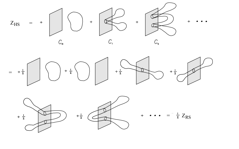
Figure 1: Method of images in target spacetime with Neumann boundary conditions. The partition function in half-space $Z_{\text{HS}}$ is one-half its counterpart in reflected (doubled) space $Z_{\text{RS}}$.

It is important to note that Whenever the worldsheet bounces from the wall, there is a contribution to the path integral. This contribution depends on the boundary conditions. For Dirichlet boundary conditions, it comes with a $(-)$ sign while for Neumann boundary conditions, it comes with a $(+)$ sign Bastianelli:2006hq ; Bastianelli:2008vh ; Bastianelli:2009mw . We will be choosing Neumann boundary condition in this work.

Consider the embedding that bounces off the wall once. The worldsheet intersects the wall in a circle. The action being an integral on the worldsheet can be split into two pieces, each for a piece emanating from the circle. Now, if we reflect the spacetime and a single piece, the action remains the same. So we get a embedding in the reflected spacetime that crosses the wall once. But, there are exactly two embeddings in the reflected target space that correspond to a single embedding in half space. The same argument holds for any number of bounces (including zero bounces). Therefore, we can express the path integral of embeddings in half-space as one half the path integral in the reflected (doubled) space. We will explore in a bit more detail the relationship between half-space and reflected space in light of reflected Brownian motion and stochastic dynamics in section 5.

$$Z_{\text{HS}} =\int_{X^{D}\geq 0}[DX]e^{-I_{\text{NLSM}}[X,\Phi,\omega,\gamma]}$$ (29)

$$=\frac{1}{2}\,Z_{\text{RS}}=\int\frac{1}{2}[DX]e^{-I_{\text{NLSM}}[X,\tilde{\Phi},\omega,\gamma]}$$

Next, we explain the set-up of the calculation of $Z_{\text{RS}}$.

3 Setup of calculation

In terms of the NLSM worldsheet action, both the metric and dilaton are reflected about the wall to the other side. The spacetime metric is flat everywhere, but the dilaton in this reflected space $\tilde{\Phi}(X^{\mu})$ is defined for $X^{D}\in\mathbb{R}$. More concretely, $\tilde{\Phi}(X^{\mu})$ is the sum of two terms, each takes values on one side of the wall

$$\tilde{\Phi}(X^{\mu})=\Phi_{0}+\tilde{\phi}(X^{\mu}) =\Phi(X^{i},X^{D})\Theta(X^{D})+\Phi(X^{i},-X^{D})\Theta(-X^{D})$$ (30)

$$=\Phi_{0}+\phi(X^{i},X^{D})\Theta(X^{D})+\phi(X^{i},-X^{D})\Theta(-X^{D}).$$

To carry out the NLSM expansion, we split the string $X^{\mu}$ into a zero mode $Y^{\mu}$ and a non-zero mode $\eta^{\mu}(z)$

$$X^{\mu}(z)=Y^{\mu}+\sqrt{\alpha^{\prime}}\eta^{\mu}(z).$$ (31)

The deformed NLSM action is given by

$$I_{\text{NLSM}} =\frac{1}{4\pi\alpha^{\prime}}\int d^{2}z\sqrt{g}\left(g^{ab}\partial_{a}X^{\mu}\partial_{b}X^{\nu}\delta_{\mu\nu}+\alpha^{\prime}R^{(2)}\tilde{\Phi}(X)\right)$$ (32)

$$=\frac{1}{4\pi\alpha^{\prime}}\int d^{2}z\sqrt{g}\left(\alpha^{\prime}g^{ab}\partial_{a}\eta^{\mu}\partial_{b}\eta^{\nu}\delta_{\mu\nu}+\alpha^{\prime}R^{(2)}\tilde{\Phi}\left(Y+\sqrt{\alpha^{\prime}}\eta\right)\right)$$ (33)

$$=\frac{1}{4\pi\alpha^{\prime}}\int d^{2}z\sqrt{g}\left(\alpha^{\prime}g^{ab}\partial_{a}\eta^{\mu}\partial_{b}\eta^{\nu}\delta_{\mu\nu}+\alpha^{\prime}R^{(2)}\Phi_{0}\right)+\frac{1}{4\pi\alpha^{\prime}}\int d^{2}z\sqrt{g}\left(\alpha^{\prime}R^{(2)}\tilde{\phi}(Y+\sqrt{\alpha^{\prime}}\eta)\right)$$ (34)

$$=\frac{1}{4\pi\alpha^{\prime}}\int d^{2}z\sqrt{g}\left(\alpha^{\prime}g^{ab}\partial_{a}\eta^{\mu}\partial_{b}\eta^{\nu}\delta_{\mu\nu}\right)+2\Phi_{0}+\frac{1}{4\pi\alpha^{\prime}}\int d^{2}z\sqrt{g}\left(\alpha^{\prime}R^{(2)}\tilde{\phi}(Y+\sqrt{\alpha^{\prime}}\eta)\right)$$ (35)

$$=I_{\text{P}}[\eta,g]+V[\eta,g,\tilde{\phi}],$$ (36)

where

$$V[\eta,g,\tilde{\phi}]=\frac{1}{4\pi}\int d^{2}z\sqrt{g}R^{(2)}\tilde{\phi}(Y+\sqrt{\alpha^{\prime}}\eta(z)).$$ (37)

The path integral measure is given by

$$[DX]=d^{D}Y[D\sqrt{\alpha^{\prime}}\eta]\,.$$ (38)

and the matter partition function in half-space becomes

$$Z_{\text{HS}} =\frac{1}{2}\int[DX]e^{-I_{\text{NLSM}}[X,\tilde{\Phi},\omega,\gamma]},$$ (39)

$$=\frac{1}{2}\int d^{D}Y\int[D\sqrt{\alpha^{\prime}}\eta]e^{-I_{\text{p}}[\eta,g]}e^{-V[\eta,g,\tilde{\phi}]}$$ (40)

$$=\frac{1}{2}\int d^{D}Y\int[D\sqrt{\alpha^{\prime}}\eta]e^{-I_{\text{p}}[\eta,g]}\left(1-V+O(V^{2})\right)$$ (41)

$$=\frac{1}{2}Z_{\text{nz}}\int d^{D}Y\left(1-\left\langle V\right\rangle+\left\langle O(V^{2})\right\rangle\right),$$ (42)

where $Z_{\text{nz}}:=\int\left[D\sqrt{\alpha^{\prime}}\eta\right]e^{-I_{\text{p}}[\eta,g]}$ is the path integral for the non-zero modes and $\left\langle V\right\rangle$ is defined by

$$\left\langle V\right\rangle=\frac{1}{Z_{\text{nz}}}\int[D\sqrt{\alpha^{\prime}}\eta]e^{-I_{\text{p}}[\eta,g]}V\,.$$ (43)

Since $\phi\ll 1$, the higher order terms in $V$ are suppressed, so we can drop the $O(V^{2})$ terms.

Now we compute $\left\langle V\right\rangle$.

$$\left\langle V\right\rangle =\frac{1}{4\pi}\int d^{2}z\sqrt{g}R^{(2)}\int[D\sqrt{\alpha^{\prime}}\eta]\,e^{-I_{\text{p}}[\eta,g]}\tilde{\phi}(Y^{\mu}+\sqrt{\alpha^{\prime}}\eta^{\mu}(z))$$ (44)

$$=\frac{1}{4\pi}\int d^{2}z\sqrt{g}R^{(2)}\left\langle\tilde{\phi}(Y^{\mu}+\sqrt{\alpha^{\prime}}\eta^{\mu}(z))\right\rangle.$$ (45)

If $Y^{\mu}$ is far away from the wall in string units, i.e. $\frac{\absolutevalue{Y^{D}}}{\sqrt{\alpha^{\prime}}}\gg 1$, then one can Taylor expand $\tilde{\phi}(X^{\mu})$ about the point $Y^{\mu}$

$$\left\langle\tilde{\phi}\left(Y^{\mu}+\sqrt{\alpha^{\prime}}\eta^{\mu}(z)\right)\right\rangle =\tilde{\phi}\left(Y^{\mu}\right)\left\langle\mathbf{1}\right\rangle+\sqrt{\alpha^{\prime}}\partial_{\mu}\tilde{\phi}\left(Y^{\mu}\right)\left\langle\eta^{\mu}(z)\right\rangle+\frac{\alpha^{\prime}}{2}\partial_{\mu}\partial_{\nu}\tilde{\phi}\left(Y^{\mu}\right)\left\langle\eta^{\mu}(z)\eta^{\nu}(z)\right\rangle+O(\alpha^{\prime 3/2}).$$ (46)

Here, $\left\langle\mathbf{1}\right\rangle=1$ and the one-point function vanishes (because it an odd integral). Then

$$\left\langle\tilde{\phi}\left(Y^{\mu}+\sqrt{\alpha^{\prime}}\eta^{\mu}(z)\right)\right\rangle =\tilde{\phi}\left(Y^{\mu}\right)+\frac{\alpha^{\prime}}{2}\partial_{\mu}\partial_{\nu}\tilde{\phi}\left(Y^{\mu}\right)\left\langle\eta^{\mu}(z)\eta^{\nu}(z)\right\rangle+O(\alpha^{\prime 3/2}).$$ (47)

It may be worth pointing out that this far-from-the-wall region where the worldsheet path integral is not restricted is the case considered in Ahmadain:2022eso , and this is the reason why there is no notion of a one-point to begin with.

However, if $Y^{\mu}$ is close to the wall, i.e $\frac{\absolutevalue{Y^{D}}}{\sqrt{\alpha^{\prime}}}\sim 1$, then the kink in $\tilde{\phi}\left(X^{i},X^{D}\right)$ at the wall does matter. In this near wall region, the dilaton will approximately be a linear function of the absolute value of $X_{D}$ on either side of the wall

$$\tilde{\phi}\left(X^{i},X^{D}\right)\approx\phi\left(X^{i},0\right)+\partial_{D}\phi\left(X^{i},0\right)\absolutevalue{X^{D}}\,,$$ (48)

where $\partial_{D}\phi\left(X^{i},0\right)$ is the right limit of the first derivative (as strictly speaking, the derivative doesn’t exist on the wall due to the kink):

$$\partial_{D}\phi\left(X^{i},0\right):=\lim_{X^{D}\to 0^{+}}\partial_{D}\phi\left(X^{i},X^{D}\right).$$ (49)

Now we can Taylor expand along the tangential direction to the wall about the point $Y^{i}$

$$\tilde{\phi}\left(Y^{i}+\sqrt{\alpha^{\prime}}\eta^{i}(z),Y^{D}+\sqrt{\alpha^{\prime}}\eta^{D}(z)\right) \approx\phi\left(Y^{i}+\sqrt{\alpha^{\prime}}\eta^{i}(z),0\right)+\partial_{D}\phi\left(Y^{i}+\sqrt{\alpha^{\prime}}\eta^{i}(z),0\right)\absolutevalue{Y^{D}+\sqrt{\alpha^{\prime}}\eta^{D}(z)}$$ (50)

$$=\phi\left(Y^{i},0\right)+\sqrt{\alpha^{\prime}}\partial_{i}\phi\left(Y^{i},0\right)\eta^{i}(z)$$ (51)

$$+\partial_{D}\phi\left(Y^{i},0\right)\absolutevalue{Y^{D}+\sqrt{\alpha^{\prime}}\eta^{D}(z)}$$ (52)

$$+\sqrt{\alpha^{\prime}}\partial_{i}\partial_{D}\phi\left(Y^{i},0\right)\eta^{i}(z)\absolutevalue{Y^{D}+\sqrt{\alpha^{\prime}}\eta^{D}(z)}+O(\alpha^{\prime}).$$ (53)

The expectation value of all terms odd in $\eta^{i}(z)$ vanishes in a free theory. Hence,

$$\left\langle\tilde{\phi}\left(Y^{\mu}+\sqrt{\alpha^{\prime}}\eta^{\mu}(z)\right)\right\rangle =\phi\left(Y^{i},0\right)+\partial_{D}\phi\left(Y^{i},0\right)\left\langle\absolutevalue{Y^{D}+\sqrt{\alpha^{\prime}}\eta^{D}(z)}\right\rangle+O(\alpha^{\prime}).$$ (54)

Thus, it is the near-wall region that leads to a non-zero one-point function in the limit ${X^{D}\to 0^{+}}$ because the wiggling part of the string $\eta^{D}(z)$ is restricted to half-space by the presence of the wall.

An explicit calculation of the exact one-point function $\left\langle\absolutevalue{Y^{D}+\sqrt{\alpha^{\prime}}\eta^{D}(z)}\right\rangle$ is presented in appendix A.

4 The classical boundary dilaton action in half-space

In this section, we put things together to compute the total classical off-shell action in half-space, $I_{\text{HS}}$, and show it obeys a well-defined variational principle for Neumann boundary conditions. We first use the result in appendix A for the one-point $\left\langle\absolutevalue{Y^{D}+\sqrt{\alpha^{\prime}}\eta^{D}(z_{0})}\right\rangle$ to write down an expression for the boundary dilaton action from the near-wall spacetime region. We then compute the bulk dilaton action $I_{\text{bulk}}$, i.e. the dilaton kinetic term, from the far-wall region. This bulk action comes with its own boundary contribution Ahmadain:2022eso . To obtain the total action, we add all bulk and boundary contributions and apply Tsyetlin’s prescriptions. We then find that the two boundary terms cancel out (as they should) and we are left with an off-shell action for the dilaton in half-space that has a well-defined variational principle for a Neumann boundary condition.

In appendix A, we show that

$$\left\langle\absolutevalue{Y^{D}+\sqrt{\alpha^{\prime}}\eta^{D}(z_{0})}\right\rangle =\sqrt{\alpha^{\prime}}\left(\frac{\sqrt{\Omega}}{\sqrt{\pi}}e^{-\frac{(Y^{D})^{2}}{\alpha^{\prime}\Omega}}+\frac{Y^{D}}{\sqrt{\alpha^{\prime}}}\text{erf}\left(\frac{Y^{D}}{\sqrt{\alpha^{\prime}\Omega}}\right)\right)$$ (55)

$$=\sqrt{\alpha^{\prime}}\left(\left\langle\absolutevalue{\eta^{D}(z_{0})}\right\rangle e^{-\frac{(Y^{D})^{2}}{\alpha^{\prime}\Omega}}+\frac{Y^{D}}{\sqrt{\alpha^{\prime}}}\text{erf}\left(\frac{Y^{D}}{\sqrt{\alpha^{\prime}\Omega}}\right)\right).$$ (56)

The sphere partition function in half-space (39) splits into two pieces, each in a different spacetime region: near the wall and far from the wall

$$Z_{\text{HS}}=\frac{1}{2}Z_{\text{nz}}V_{Y^{D}}+Z_{\text{near}}+Z_{\text{far}}+O(V^{2})\,,$$ (57)

where $V_{Y^{D}}=\int d^{D}Y$ and

$$Z_{\text{near}} :=\frac{1}{2}Z_{\text{nz}}\int_{\frac{\absolutevalue{Y^{D}}}{\sqrt{\alpha^{\prime}}}\sim 1}d^{D}Y\left(-\frac{1}{4\pi}\int d^{2}z\sqrt{g}R^{(2)}\left\langle\tilde{\phi}(Y^{\mu}+\sqrt{\alpha^{\prime}}\eta^{\mu}(z))\right\rangle\right).$$ (58)

$$Z_{\text{far}} :=\frac{1}{2}Z_{\text{nz}}\int_{\frac{\absolutevalue{Y^{D}}}{\sqrt{\alpha^{\prime}}}\gg 1}d^{D}Y\left(-\frac{1}{4\pi}\int d^{2}z\sqrt{g}R^{(2)}\left\langle\tilde{\phi}(Y^{\mu}+\sqrt{\alpha^{\prime}}\eta^{\mu}(z))\right\rangle\right).$$ (59)

Far from the wall, $Z_{\text{far}}$ gives the bulk contribution to the action while, due to the presence of the wall, $Z_{\text{near}}$ gives an additional contribution which is given by

$$Z_{\text{near}} :=\frac{1}{2}Z_{\text{nz}}\int_{\frac{\absolutevalue{Y^{D}}}{\sqrt{\alpha^{\prime}}}\sim 1}d^{D}Y\left(-\frac{1}{4\pi}\int d^{2}z\sqrt{g}R^{(2)}\left(\phi\left(Y^{i},0\right)+\partial_{D}\phi\left(Y^{i},0\right)\left\langle\absolutevalue{Y^{D}+\sqrt{\alpha^{\prime}}\eta^{D}(z)}\right\rangle+O(\alpha^{\prime})\right)\right)$$ (60)

$$=\frac{1}{2}Z_{\text{nz}}\int_{\frac{\absolutevalue{Y^{D}}}{\sqrt{\alpha^{\prime}}}\sim 1}d^{D}Y\left(-\frac{1}{4\pi}\int d^{2}z\sqrt{g}R^{(2)}\left(\phi\left(Y^{i},0\right)+O(\alpha^{\prime})\right)\right)+Z_{\text{wall}}\,,$$ (61)

where $Z_{\text{wall}}$ is

$$Z_{\text{wall}} =\frac{1}{2}Z_{\text{nz}}\int_{\frac{\absolutevalue{Y^{D}}}{\sqrt{\alpha^{\prime}}}\sim 1}d^{D}Y\left(-\frac{1}{4\pi}\int d^{2}z\sqrt{g}R^{(2)}\partial_{D}\phi\left(Y^{i},0\right)\left\langle\absolutevalue{Y^{D}+\sqrt{\alpha^{\prime}}\eta^{D}(z)}\right\rangle\right)$$ (62)

$$=\frac{1}{2}Z_{\text{nz}}\int_{\frac{\absolutevalue{Y^{D}}}{\sqrt{\alpha^{\prime}}}\sim 1}d^{D}Y(-2)\partial_{D}\phi\left(Y^{i},0\right)\left\langle\absolutevalue{Y^{D}+\sqrt{\alpha^{\prime}}\eta^{D}(z)}\right\rangle$$ (63)

$$=-\frac{1}{2}\times 2Z_{\text{nz}}\int d^{D-1}Y\ \partial_{D}\phi\left(Y^{i},0\right)\int_{\frac{\absolutevalue{Y^{D}}}{\sqrt{\alpha^{\prime}}}\sim 1}dY^{D}\sqrt{\alpha^{\prime}}\left(\frac{\sqrt{\Omega}}{\sqrt{\pi}}e^{-\frac{(Y^{D})^{2}}{\alpha^{\prime}\Omega}}+\frac{Y^{D}}{\sqrt{\alpha^{\prime}}}\text{erf}\left(\frac{Y^{D}}{\sqrt{\alpha^{\prime}\Omega}}\right)\right).$$ (64)

The integrand in (64) is valid only near the wall where $Y^{D}\sim\sqrt{\alpha^{\prime}}$ and thus we integrate it from $-\frac{Y_{c}\sqrt{\alpha^{\prime}}}{2}$ to $\frac{Y_{c}\sqrt{\alpha^{\prime}}}{2}$ where the cutoff $Y_{c}$ is a dimensionless constant.

$$Z_{\text{wall}} =-\frac{1}{2}\times 2Z_{\text{nz}}\int d^{D-1}Y\ \partial_{D}\phi\left(Y^{i},0\right)\int_{-\frac{Y_{c}\sqrt{\alpha^{\prime}}}{2}}^{\frac{Y_{c}\sqrt{\alpha^{\prime}}}{2}}dY^{D}\sqrt{\alpha^{\prime}}\left(\frac{\sqrt{\Omega}}{\sqrt{\pi}}e^{-\frac{(Y^{D})^{2}}{\alpha^{\prime}\Omega}}+\frac{Y^{D}}{\sqrt{\alpha^{\prime}}}\text{erf}\left(\frac{Y^{D}}{\sqrt{\alpha^{\prime}\Omega}}\right)\right)$$ (65)

$$=-\frac{1}{2}\times 2Z_{\text{nz}}\int d^{D-1}Y\ \partial_{D}\phi\left(Y^{i},0\right)2\int_{0}^{\frac{Y_{c}\sqrt{\alpha^{\prime}}}{2}}dY^{D}\sqrt{\alpha^{\prime}}\left(\frac{\sqrt{\Omega}}{\sqrt{\pi}}e^{-\frac{(Y^{D})^{2}}{\alpha^{\prime}\Omega}}+\frac{Y^{D}}{\sqrt{\alpha^{\prime}}}\text{erf}\left(\frac{Y^{D}}{\sqrt{\alpha^{\prime}\Omega}}\right)\right)$$ (66)

$$=-\frac{1}{2}\times 2Z_{\text{nz}}\int d^{D-1}Y\ \partial_{D}\phi\left(Y^{i},0\right)\frac{\alpha^{\prime}}{4}\left(\frac{2e^{-\frac{Y_{c}^{2}}{4\Omega}}Y_{c}\sqrt{\Omega}}{\sqrt{\pi}}+(Y_{c}^{2}+2\Omega)\text{erf}\left(\frac{Y_{c}}{2\sqrt{\Omega}}\right)\right).$$ (67)

Expanding near $Y_{c}\to\infty$ and keeping only the leading and subleading terms, the first term vanishes and $\operatorname{erf}\left(\frac{Y_{c}}{2\sqrt{\Omega}}\right)\rightarrow 1$ and thus we obtain

$$Z_{\text{wall}} =-\frac{1}{2}\times 2Z_{\text{nz}}\int d^{D-1}Y\ \partial_{D}\phi\left(Y^{i},0\right)\left(\frac{\alpha^{\prime}Y_{c}^{2}}{4}+\frac{\alpha^{\prime}\Omega}{2}\right).$$ (68)

There is a factor of $e^{-2\Phi_{0}}$ sitting inside $Z_{\text{nz}}$. Extracting it gives $Z_{\text{nz}}=\tilde{Z}_{\text{nz}}e^{-2\Phi_{0}}$, where $\tilde{Z}_{\text{nz}}$ does not depend on the dilaton

$$Z_{\text{wall}} =-\frac{1}{2}\times 2\tilde{Z}_{\text{nz}}\int d^{D-1}Y\ e^{-2\Phi_{0}}\partial_{D}\phi\left(Y^{i},0\right)\left(\frac{\alpha^{\prime}Y_{c}^{2}}{4}+\frac{\alpha^{\prime}\Omega}{2}\right).$$ (69)

We can express the derivative of $\phi$ as the derivative of $\Phi$ (as $\Phi_{0}$ is just a constant) and also replace $e^{-2\Phi_{0}}$ with $e^{-2\Phi}$ (as the difference will just be higher order) to finally get

$$Z_{\text{wall}} =-\frac{1}{2}\times 2\tilde{Z}_{\text{nz}}\int d^{D-1}Y\ e^{-2\Phi}\partial_{D}\Phi\left(Y^{i},0\right)\left(\frac{\alpha^{\prime}Y_{c}^{2}}{4}+\frac{\alpha^{\prime}\Omega}{2}\right).$$ (70)

Using that $\Omega=-2\ln{\epsilon}$, $Z_{\text{wall}}$ takes the final form

$$Z_{\text{wall}} =-\frac{1}{2}\times 2\tilde{Z}_{\text{nz}}\,\alpha^{\prime}\int d^{D-1}Y\ e^{-2\Phi}\partial_{D}\Phi\left(Y^{i},0\right)\left(\frac{Y_{c}^{2}}{4}+\frac{-2\ln{\epsilon}}{2}\right).$$ (71)

The above form should be familiar. It has a structure similar to that of the bulk sphere partition function: there is an overall log divergence multiplying the boundary dilaton sphere effective action.

As in the bulk off-shell action, we apply Tseytlin’s prescription $\frac{\partial}{\partial\log{\epsilon}}$ to eliminate overall the log divergence and the divergent $Y_{c}^{2}$ term to obtain the classical off-shell boundary action of the dilaton in half-space

$$I_{\text{wall}}=-\frac{\partial}{\partial\log{\epsilon}}Z_{\text{wall}}=-\alpha^{\prime}\tilde{Z}_{\text{nz}}\int d^{D-1}Y\ e^{-2\Phi}\partial_{D}\Phi\left(Y^{i},0\right)=+\alpha^{\prime}\tilde{Z}_{\text{nz}}\int d^{D-1}Y\ e^{-2\Phi}\partial_{n}\Phi\left(Y^{i},0\right),$$ (72)

where $\partial_{n}$ is the normal derivative in the direction of the outward-pointing normal $n^{\mu}$ i.e. $\partial_{n}=-\partial_{D}$.

Now, we compute $Z_{\text{far}}$ to obtain the bulk contribution to $Z_{\text{HS}}$

$$Z_{\text{far}} =\frac{1}{2}Z_{\text{nz}}\int_{\frac{\absolutevalue{Y^{D}}}{\sqrt{\alpha^{\prime}}}\gg 1}d^{D}Y\left(-\frac{1}{4\pi}\int d^{2}z\sqrt{g}R^{(2)}\left\langle\tilde{\phi}(Y^{\mu}+\sqrt{\alpha^{\prime}}\eta^{\mu}(z))\right\rangle\right)$$ (73)

$$=\frac{1}{2}Z_{\text{nz}}\int_{\frac{\absolutevalue{Y^{D}}}{\sqrt{\alpha^{\prime}}}\gg 1}d^{D}Y\left(-\frac{1}{4\pi}\int d^{2}z\sqrt{g}R^{(2)}\left(\tilde{\phi}\left(Y^{\mu}\right)+\frac{\alpha^{\prime}}{2}\partial_{\mu}\partial_{\nu}\tilde{\phi}\left(Y^{\mu}\right)\left\langle\eta^{\mu}(z)\eta^{\nu}(z)\right\rangle+O(\alpha^{\prime 3/2})\right)\right).$$ (74)

Keeping only the relevant term (with a log ${\epsilon}^{-1}$ coefficient) in $Z_{\text{far}}$ is

$$Z_{\text{far}} =\frac{1}{2}Z_{\text{nz}}\int_{\frac{\absolutevalue{Y^{D}}}{\sqrt{\alpha^{\prime}}}\gg 1}d^{D}Y\left(-\frac{1}{4\pi}\int d^{2}z\sqrt{g}R^{(2)}\frac{\alpha^{\prime}}{2}\partial_{\mu}\partial_{\nu}\tilde{\phi}\left(Y^{\mu}\right)\delta^{\mu\nu}\left(-\log{\epsilon}+O({\epsilon}^{2})\right)\right).$$ (75)

Applying Tseytlin’s prescription to $Z_{\text{far}}$ gives $I_{\text{bulk}}$

$$I_{\text{bulk}}:=I_{\text{far}} =-\frac{\partial}{\partial\log{\epsilon}}Z_{\text{far}}$$ (76)

$$=-\frac{1}{2}Z_{\text{nz}}\frac{\alpha^{\prime}}{2}\int_{\frac{\absolutevalue{Y^{D}}}{\sqrt{\alpha^{\prime}}}\gg 1}d^{D}Y\left(\frac{1}{4\pi}\int d^{2}z\sqrt{g}R^{(2)}\partial^{2}\tilde{\phi}\left(Y^{\mu}\right)\right)$$ (77)

$$=-\frac{2}{2}Z_{\text{nz}}\frac{\alpha^{\prime}}{2}\int_{\frac{Y^{D}}{\sqrt{\alpha^{\prime}}}\gg 1}d^{D}Y\left(\frac{1}{4\pi}\int d^{2}z\sqrt{g}R^{(2)}\partial^{2}\tilde{\phi}\left(Y^{\mu}\right)\right)$$ (78)

$$=-\frac{2}{2}Z_{\text{nz}}\frac{\alpha^{\prime}}{2}\int_{\frac{Y^{D}}{\sqrt{\alpha^{\prime}}}\gg 1}d^{D}Y\left(\frac{8\pi}{4\pi}\partial^{2}\tilde{\phi}\left(Y^{\mu}\right)\right)$$ (79)

$$=-\tilde{Z}_{\text{nz}}\alpha^{\prime}\int_{\frac{Y^{D}}{\sqrt{\alpha^{\prime}}}\gg 1}d^{D}Ye^{-2\Phi}\partial^{2}\Phi$$ (80)

This free action for the dilaton (80) does not have a well-defined variational principle since upon variation, it gives

$$\delta I_{\text{bulk }} =2\alpha^{\prime}\tilde{Z}_{\text{nz}}\int_{\frac{Y^{D}}{\sqrt{\alpha^{\prime}}}\gg 1}d^{D}Y\left[e^{-2\Phi}\partial^{2}\Phi+\partial_{\mu}\left(e^{-2\Phi}\partial^{\mu}\Phi\right)\right]\delta\Phi$$

$$-\alpha^{\prime}\tilde{Z}_{\text{nz}}\int_{\partial\mathcal{M}}d^{D-1}Ye^{-2\Phi}\,\delta(\partial_{n}\Phi)-2\alpha^{\prime}\tilde{Z}_{\text{nz}}\int_{\partial\mathcal{M}}d^{D-1}Ye^{-2\Phi}\partial_{n}\Phi\,\delta\Phi.$$ (81)

The first term in (81) is the bulk dilaton equation of motion while the second and third are boundary terms. The second boundary term in (81) is where we impose boundary conditions on $\Phi\left(Y^{i},0\right)$. It vanishes for Dirichlet boundary conditions ($\delta\Phi=0$) while imposing Neumann boundary conditions ($\partial_{n}\Phi=0$) guarantees a consistent boundary equation of motion. However, this is true only if the dilaton $\Phi\left(Y^{i},0\right)$ satisfies the boundary conditions on the wall. In our case, it does not simply because $\Phi\left(Y^{i},0\right)$ is off-shell. The first boundary term is what spoils the variational principle. It is the GHY-like term of the free two-derivative action (80) which must be accounted for, i.e. by adding an additional boundary term whose variation exactly cancels with it to have a well-posed variational principle. This additional boundary term is $I_{\text{wall}}$ in (72). Let’s see how this works.

The total classical off-shell string action for the dilaton in half-space is the sum of bulk and boundary contributions (72)

$$I_{\text{sphere}}:=I_{\text{HS}} =I_{\text{bulk}}+I_{\text{wall}}$$

$$=-\tilde{Z}_{\text{nz}}\alpha^{\prime}\int_{\frac{Y^{D}}{\sqrt{\alpha^{\prime}}}\gg 1}d^{D}Ye^{-2\Phi}\partial^{2}\Phi+\alpha^{\prime}\tilde{Z}_{\text{nz}}\int d^{D-1}Y\ e^{-2\Phi}\partial_{n}\Phi\left(Y^{i},0\right)$$ (82)

$$=-2\tilde{Z}_{\text{nz}}\alpha^{\prime}\int_{\frac{Y^{D}}{\sqrt{\alpha^{\prime}}}\gg 1}d^{D}Ye^{-2\Phi}\partial_{\mu}\Phi\partial^{\mu}\Phi,$$ (83)

where integration by parts is used to get the last line.

Varying $I_{\text{sphere}}$ gives

$$\delta I_{\text{sphere}}= \,\delta I_{\text{bulk }}+\delta I_{\text{wall}}$$

$$=2\alpha^{\prime}\tilde{Z}_{\text{nz}}\int_{\frac{Y^{D}}{\sqrt{\alpha^{\prime}}}\gg 1}d^{D}Y\left[e^{-2\Phi}\partial^{2}\Phi+\partial_{\mu}\left(e^{-2\Phi}\partial^{\mu}\Phi\right)\right]\delta\Phi$$ (84)

$$-\alpha^{\prime}\tilde{Z}_{\text{nz}}\int_{\partial\mathcal{M}}d^{D-1}Ye^{-2\Phi}\,\delta(\partial_{n}\Phi)+\alpha^{\prime}\tilde{Z}_{\text{nz}}\int_{\partial\mathcal{M}}d^{D-1}Ye^{-2\Phi}\,\delta(\partial_{n}\Phi)$$ (85)

$$-4\alpha^{\prime}\tilde{Z}_{\text{nz}}\int_{\partial\mathcal{M}}d^{D-1}Ye^{-2\Phi}\partial_{n}\Phi\,\delta\Phi$$ (86)

$$=2\alpha^{\prime}\tilde{Z}_{\text{nz}}\int_{\frac{Y^{D}}{\sqrt{\alpha^{\prime}}}\gg 1}d^{D}Y\left[e^{-2\Phi}\partial^{2}\Phi+\partial_{\mu}\left(e^{-2\Phi}\partial^{\mu}\Phi\right)\right]\delta\Phi-4\alpha^{\prime}\tilde{Z}_{\text{nz}}\int_{\partial\mathcal{M}}d^{D-1}Ye^{-2\Phi}\partial_{n}\Phi\,\delta\Phi.$$ (87)

In the second line, we notice that the variation $\delta I_{\text{wall}}$ exactly cancels its counterpart in $\delta I_{\text{bulk}}$ i.e. $e^{-2\Phi}\,\delta(\partial_{n}\Phi)$ such that we are left in the end with only the bulk and boundary dilaton equations of motion. Therefore, $I_{\text{sphere}}$ has a well-defined variational principle only with the addition of $I_{\text{wall}}$ as a boundary term.
 
This is the main result of this paper.

4.1 The classical on-shell action

Let us now impose the dilaton bulk equation of motion in $I_{\text{bulk}}$ to obtain the on-shell action. To do that, we first integrate by parts (80) before varying to obtain

$$I_{\text{bulk}} =-\tilde{Z}_{\text{nz}}\alpha^{\prime}\int_{\frac{Y^{D}}{\sqrt{\alpha^{\prime}}}\gg 1}d^{D}Ye^{-2\Phi}\partial^{2}\Phi$$ (88)

$$=-\tilde{Z}_{\text{nz}}\alpha^{\prime}\int_{\frac{Y^{D}}{\sqrt{\alpha^{\prime}}}\gg 1}d^{D}Y\,\partial_{\mu}\left(e^{-2\Phi}\partial^{\mu}\Phi\right)-2\tilde{Z}_{\text{nz}}\alpha^{\prime}\int_{\frac{Y^{D}}{\sqrt{\alpha^{\prime}}}\gg 1}d^{D}Ye^{-2\Phi}(\partial\Phi)^{2}$$ (89)

$$=-\tilde{Z}_{\text{nz}}\alpha^{\prime}\int d^{D-1}Ye^{-2\Phi}\partial_{n}\Phi-2\tilde{Z}_{\text{nz}}\alpha^{\prime}\int_{\frac{Y^{D}}{\sqrt{\alpha^{\prime}}}\gg 1}d^{D}Ye^{-2\Phi}(\partial\Phi)^{2}\,.$$ (90)

Imposing the dilaton equation of motion in $I_{\text{bulk}}$

$$e^{-2\Phi}(\partial\Phi)^{2}=-\partial_{\mu}\left(e^{-2\Phi}\partial^{\mu}\Phi\right)$$ (91)

leaves us with the following bulk action

$$I_{\text{bulk}}=+\tilde{Z}_{\text{nz}}\alpha^{\prime}\int d^{D-1}Ye^{-2\Phi}\partial_{n}\Phi$$ (92)

The classical on-shell action for the dilaton in half-space is therefore the sum of the two boundary contributions (92) and (72)

$$I_{\text{sphere}}:=I_{\text{HS}} =I_{\text{bulk}}+I_{\text{wall}}$$ (93)

$$=2\,\alpha^{\prime}\tilde{Z}_{\text{nz}}\int d^{D-1}Ye^{-2\Phi}\partial_{n}\Phi=2I_{\text{wall}}\,.$$ (94)

Therefore, we observe that the two boundary terms in $I_{\text{sphere}}$ add up to give the on-shell classical action.

Note that if we impose the boundary equation for the motion for the dilaton, i.e. the Neumann boundary condition, then $I_{\text{wall}}=0$ and hence $I_{\text{sphere}}=0$. This is of course another way to say our worldsheet derivation of $I_{\text{wall}}$ from the outset is off-shell.

5 Discussion

In this section, we begin by making the observation that the $N$-th point correlation function $\left\langle\absolutevalue{\eta^{D}(z_{0})}^{N}\right\rangle$ in (186)

$$\left\langle\absolutevalue{\eta^{D}(z_{0})}^{N}\right\rangle =\frac{1}{\sqrt{\pi}}\Gamma\left(\frac{1+N}{2}\right)\Omega^{N/2}\,,$$ (95)

equals the $N$-th moment of the half-normal distribution for the absolute value of a random variable $|X|$. We will comment on the relationship between the two quantities as well as the relationship between the string’s zero and nonzero mode to reflected Brownian motion and one-dimensional random walks in spaces with a totally reflecting barrier. We begin first by defining the half-normal distribution and its main properties.

Let $X_{t}$ be a normally distributed random variable with a standard deviation $t\in[0,\infty)$. The half-normal distribution is a one-parameter scale family of distributions with scale (time) parameter $t$ which is closed under scale transformations in the sense that for $t\in[0,\infty)$, $Y_{t}=t|X_{t}|$. If $t=1$, then $Y_{t}$ has the standard half-normal distribution.

The probability density function (PDF) $f(y;t)$ of $Y$ with scale parameter $\sigma$ is given by

$$f(y;t)=\frac{1}{t}\sqrt{\frac{2}{\pi}}\exp\left(-\frac{y^{2}}{2t^{2}}\right),\quad y\in[0,\infty)\,,$$ (96)

while the cumulative distribution function (CDF) $F(y;t)$ is

$$F(y;t)=\int_{0}^{y}\frac{1}{t}\sqrt{\frac{2}{\pi}}\exp\left(-\frac{x^{2}}{2t^{2}}\right)\,dx\,.$$ (97)

Changing variables to $w=x/(\sqrt{2}t)$, the CDF can be written as

$$\mathbb{P}\left(Y_{t}\leq y\right):=F_{Y}(y;t)=\operatorname{erf}\left(\frac{y}{\sqrt{2}t}\right).$$ (98)

For any (even or odd) $N\geq 0$, the absolute central moments are given by HNDMathWorks

$$\left\langle Y_{t}^{N}\right\rangle=\left\langle|X|_{t}^{N}\right\rangle =t^{N}\cdot\frac{2^{N/2}\Gamma\left(\frac{N+1}{2}\right)}{\sqrt{\pi}},$$ (99)

with variance $\operatorname{var}(Y_{t})=t^{2}\left(1-\frac{2}{\pi}\right)$. For $N=1$, $\left\langle|X|\right\rangle=\frac{t\sqrt{2}}{\sqrt{\pi}}$ is the mean of the half-normal distribution.

Comparing (95) with (99), and using $\Omega=2\log{\epsilon}^{-1}$, we observe that they are identical

$$\left\langle\absolutevalue{\eta^{D}(z_{0})}^{N}\right\rangle=\left\langle\absolutevalue{X}_{t}^{N}\right\rangle\,,$$ (100)

once we identify the scale parameter of the distribution $t$ with the square root of the log of the worldsheet UV cutoff ${\epsilon}$

$$t\sqrt{2}=\sqrt{\Omega}=\sqrt{-\log{\epsilon}}\,\sqrt{2},\quad\textrm{and hence,}\quad t=\sqrt{-\log{\epsilon}}\,.$$ (101)

In particular, the one-point function of the string nonzero mode $\absolutevalue{\eta^{D}}$ is trivially equal to the first moment $(N=1)$ of $\absolutevalue{X_{t}}$

$$\left\langle\absolutevalue{\eta^{D}(z_{0})}\right\rangle=\left\langle\absolutevalue{X_{t}}\right\rangle=\frac{t\sqrt{2}}{\sqrt{\pi}}.$$ (102)

This observation gives a probabilistic interpretation of $I_{\text{HS}}$ and connects it to the vast and interesting literature on the theory of reflecting Brownian motion morters2010brownian ; karatzas2014brownian . Specifically, the half-normal distribution naturally appears in the theory of reflected Brownian motion (RBM) of stochastic (Wiener) processes of $\left\langle\absolutevalue{X_{t}}\right\rangle$ in spaces with reflecting boundaries. It arises as the probability distribution for the local boundary time levy1965processus ; it1965diffusion ; lions1984stochastic ; saisho1987stochastic ; hsu1985probabilistic and running maximum morters2010brownian ; karatzas2014brownian ; borodin2015handbook ; grebenkov2019probability . See also random . In banderier2018local ; wallner2020half , it is also shown that the half-normal distribution emerges as the limit law for the local time at $x=0$ in directed lattice path on $\mathbb{Z}$ with no drift. The local time at zero in this type of random walk is the sum the number of returns to zero and number of $x$-axis crossings.

After giving a short introduction to the probabilistic interpretations of boundary conditions in section 5.1, we give in section 5.2 a lightening overview of reflected Brownian motion (RBM), the Skorokhod construction skorokhod1961stochastic ; skorokhod1962stochastic , Tanakas’s formula tanaka1979stochastic and the important notion of local boundary time at a point $x$ $L^{x}_{t}$ levy1965processus ; it1965diffusion .

We will then argue in section 5.3 that $\absolutevalue{\sqrt{\alpha^{\prime}}\eta^{D}(z)}$ has the same probability distribution of the boundary local time and that

$$\left\langle\absolutevalue{\sqrt{\alpha^{\prime}}\eta^{D}(z)}\right\rangle=\left\langle L^{x}_{t}\right\rangle,$$ (103)

thereby giving a purely probabilistic (random walk) description of the string dynamics in target spacetime.

We would like to comment on the fact that the value of the square root of the worldsheet length (UV) cutoff ${\epsilon}^{-1}$ acts in target space as a dial that controls the overall scale $t$ of the half-normal distribution. Each value of ${\epsilon}^{-1}$ describes a worldsheet theory at a particular renormalization group (RG) scale. Fig. 2 shows the PDF and CDF of the half-normal probability distribution with different scale parameter $t=\sqrt{-\log{\epsilon}}$. The plots can be interpreted as the RG flow from the UV with larger value of ${\epsilon}^{-1}$ (or smaller value of $\log{\epsilon}^{-1}$) to the IR with a small value of ${\epsilon}^{-1}\rightarrow 0$. The RG flow renormalizes the length of the Euclidean Schwinger propagator or equivalently the Schwinger time, as the worldsheet theory flows from the UV to the IR. The $\log{\epsilon}^{-1}\rightarrow 0$ limit corresponds to the S-matrix regime whereas, when $\log{\epsilon}^{-1}\rightarrow 0$ when (${\epsilon}\sim 1$), the worldsheet theory is in the extreme UV limit where the worldsheet theory is nonlocal Ahmadain:2022tew . The latter is the limit where the string nonzero mode $\left\langle\absolutevalue{\eta(z)}\right\rangle$ vanishes and thus, $\eta^{D}(z)$ spends all its time (with probability 1) at the boundary $X_{D}=0$.

To establish a more visible connection between the value of $\log{\epsilon}^{-1}$ and RG time, we note that the solution to one-dimensional heat diffusion equation

$$\frac{\partial k}{\partial t}=\frac{\partial^{2}k}{\partial x^{2}}\,,$$ (104)

with a step function as the initial condition

$$k(x,0)=\begin{cases}0\ \ \ \ \text{if}\ \ x<0\\ 1\ \ \ \ \text{if}\ \ x>0\\ \end{cases},$$ (105)

is given by

$$k(x,t)=\frac{1}{2}\left[1-\text{erf}\left(\frac{x}{\sqrt{4t}}\right)\right],$$ (106)

for $x\in\mathbb{R}$ and $t>0$. This solution satisfies the heat equation and approaches the initial condition as $t\rightarrow 0^{+}$. It shows how the initial discontinuity (kink) at $x=0$ diffuses (renormalized) over time, gradually smoothing out the step transition from $k=0$ to $k=1$ as heat spreads out into the bulk. Note that except right at the boundary at $x=0$, the motion $k(x,t)$ is standard Brownian. The discontinuity at the $x=0$ breaks the the spatial homogeneity assumption of standard Brownian motion. In other words, scale invariance is broken at the target space boundary. This is a fundamental principle of the reflected Brownian motion. In a distributional sense, function $k(x,t=t_{0})$ corresponds to the dilaton $\tilde{\Phi}(Y^{i},0)$.

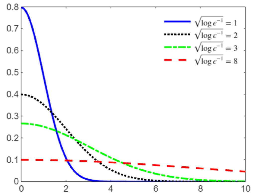
(a) The half-normal PDF

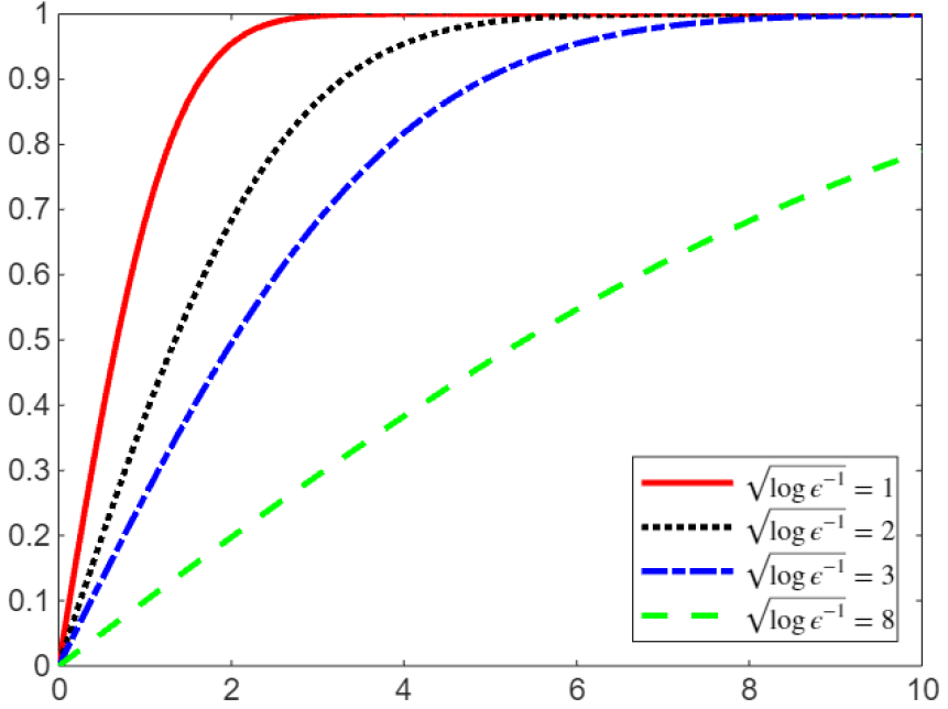
(b) The half-normal CDF

Figure 2: The half-normal probability density $f(y;t)$ and cumulative distribution $F(y;t)$ functions for different scale parameters $t=\sqrt{\log{\epsilon}^{-1}}$. The effect of changing the value of the UV position cutoff ${\epsilon}$ is to change the overall size of the distribution. A larger value of $t$ (or equivalently, a smaller value of ${\epsilon}$) brings the probability density on the left closer to a delta function and distribution on the right closer to a step function $\theta(Y)$. In terms of the local boundary time (113), a larger ${\epsilon}$ is a less diffusive regime that describes a typical string (in the distribution) $\eta^{D}(z_{0})$ which is more bound to the wall at $X^{D}=0$, i.e. spends most of its time in the near the wall within a string length $\sqrt{\alpha^{\prime}}$. In this region, the string hits the wall several times before getting diffused away. Contrast this with other distributions with smaller values of ${\epsilon}$ where the string is less localized to the boundary in a more diffusive medium. Figures adapted from https://www.mathworks.com/help/stats/half-normal-distribution.html.

5.1 The probabilistic interpretations of boundary conditions

It is well known that with a Neumann boundary condition at $x=a$, $\frac{\partial k}{\partial x}\Big{|}_{x=a}=0$, the solution to the one-dimensional heat kernel equation is the sum of $k(x,t)+k(x-a,t)$ since reflecting about the line $x=a$, we simply have

$$\frac{\partial k}{\partial x}\Big{|}_{x=a} =k(x,t)\Big{|}_{x=a}+k(x-a,t)\Big{|}_{x=a}$$ (107)

$$=k(x,t)\Big{|}_{x=a}+k(a-x,t)\Big{|}_{x=a}$$ (108)

$$=k(x,t)\Big{|}_{x=a}-k(x,t)\Big{|}_{x=a}=0\,,$$ (109)

where $k(x,t)=\frac{1}{2\sqrt{t}}\exp(-x^{2}/4t)$ is the solution with no boundaries and a delta function $\delta(x-a)$ as an initial condition. With Dirichlet boundary condition on the other hand, it is the difference instead $k(x,t)-k(x-a,t)$ that satisfies $k(a,t)=0$, as can be easily checked.

The probabilistic interpretations of boundary conditions e.g. Neumann hsu1985probabilistic and Dirichlet boundary conditions provide a fascinating link between stochastic processes, particularly Brownian motion, and partial differential equations. These interpretations can offer intuitive insights into how boundary conditions affect the behavior of random walks or diffusions, which parallel solutions to PDEs under similar conditions.

Neumann boundary conditions specify the derivative of a function along the boundary of its domain $D$, typically the normal derivative. In probabilistic terms, Neumann boundary conditions are totally reflecting barriers, in the sense that particle paths of a Brownian motion or another diffusion process (or in our case string worldsheets) that reach the wall are reflected instantaneously back into $D$ with probability 1.

Dirichlet boundary conditions, on the other hand, specify the value of a function at the boundary of its domain. In the context of stochastic processes, Dirichlet boundary conditions correspond to the behavior of absorbing barriers where the paths of Brownian motion are totally absorbed and the random process completely stops upon reaching the boundary $\partial D$ chung1995killed .

Reflected Brownian motion is the formal mathematical framework used to describe this probabilistic interpretation of the stochastic string dynamics in target spacetime. This is what we review next.

5.2 Reflected Brownian motion, local boundary time and running maximum

In this section, we give the bare minimum review of reflected Brownian motion and the associated notion of boundary local time. We will state known results, propositions and theorems without proof and omit any discussion of mathematical subtleties. However, plenty of references will be given for the readers interested in the details.

Let $\boldsymbol{X}=\left\{X_{t}:t\in[0,\infty)\right\}$ be a standard Brownian motion (Weiner) process and let $S_{t}=\sup_{s\leq t}\textbf{X}_{s}$ of $\boldsymbol{X}$ be the maximum value of $\boldsymbol{X}$ on the interval $[0,t]$. Then, the reflection principle states that if $X_{t}$ is a Brownian motion and $T$ is the time at which $X_{t}$ first hits level $a>0$, then the reflected process defined by

$$X^{\prime}(t)=\begin{cases}X_{t}&\text{ if }t<T,\\ 2X_{T}-X_{t}&\text{ if }t\geq T,\end{cases}$$ (110)

is also a Brownian motion. This principle is used to derive properties of Brownian motion, including the distribution of $S_{t}$ over certain intervals. Specifically, it refers to a lemma that states

$$\mathbb{P}\left(S_{t}\geq a\right)=2\mathbb{P}(W(t)\geq a)$$ (111)

The boundary local time levy1965processus ; it1965diffusion ; mckean1969stochastic is the quantity that encodes all the boundary physics. It is the term you add to a (stochastic) differential equation or a classical action to impose a specific boundary condition in spaces with boundaries. It represents the amount of time that a stochastic process, such as Brownian motion, spends at a boundary of its domain. In more technical terms, it quantifies the intensity or of the path’s contact with the boundary.

In path integrals, the exponential of the boundary local time gives the total probability of particle paths reflecting from the wall Clark1980half . In reflected Brownian motion, for example, it ensures that worldlines of particles (and of course string worldsheets) in a diffusive medium do not cross a reflecting boundary, i.e. reflected off the boundary. Let us make this notion a bit more precise and see how it relates to $\left\langle\absolutevalue{\eta^{D}(z)}\right\rangle$.

The boundary local time measures the amount of time a Brownian motion $\boldsymbol{X}$ spends at level $x$. Informally, it is defined as

$$L^{x}_{t}=\int_{0}^{t}\delta_{x}\left(X_{s}\right)ds.$$ (112)

A more formal definition of $L_{t}$ is given in terms of the limit of the occupation time $T_{t}$ of the Brownian motion $\textbf{X}_{t}$ in a region $\varepsilon$ near the boundary $\partial\mathcal{M}_{\varepsilon}=\{X_{t}\in\mathcal{M}:|x-\partial\mathcal{M}|<\varepsilon\}$

$$L_{t}=\lim_{\varepsilon\rightarrow 0}\frac{1}{2\varepsilon}\int_{0}^{t}ds\,\mathbb{1}_{\partial\mathcal{M}_{\varepsilon}}\left({X}_{s}\right),$$ (113)

where $\mathbb{1}_{\partial\mathcal{M}_{\varepsilon}}(X_{s})$ is the indicator function of the boundary (i.e., $\mathbb{I}_{\partial\mathcal{M}_{\varepsilon}}(X_{t})=1$ if $X_{t}\in\partial\mathcal{M}_{\varepsilon}$, and 0 otherwise). With this definition, the local boundary time $L_{t}$ measures the amount of time $X_{t}$ spends in a region $\varepsilon$ near the boundary $\partial\mathcal{M}$, and thus increases only when ${X}_{s}\in\partial\mathcal{M}_{\varepsilon}$.

A reflected Brownian motion $Z$ is a Brownian process $X$ regulated by another process $F$ such that $Z$ remains always positive. More precisely, if the process $X:\mathbb{R}\rightarrow\mathbb{R}$, the Skorokhod construction skorokhod1961stochastic ; skorokhod1962stochastic guarantees that there always exists a pair of functions $Z,F$ such that

$$Z_{t}=X_{t}+F_{t}(X)\geq 0,\quad\text{for all }t\geq 0\,.$$ (114)

The process $F_{t}$ is nondecreasing with $F_{0}=0$ and increases only when $Z_{t}$ reaches the boundary, i.e. when $Z_{t}=0$. Intuitively, $F_{t}$ pushes the process $X_{t}$ away from the boundary such that $Z_{t}$ is always positive at any point in time.

All three processes $Z_{t}$, $X_{t}$ and $F_{t}$ appear in Skorokhod stochastic differential equation skorokhod1961stochastic that describes motion in spaces ($R^{D}$) with reflecting obstacles lions1984stochastic

$$dZ_{t}=dX_{t}+\boldsymbol{n}\left(X_{t}\right)\mathbb{1}_{\partial\mathcal{M}}\left(X_{t}\right)dL_{t},\quad\text{with }Z_{0}=z_{0}\,,$$ (115)

where $\boldsymbol{n}\left(X_{t}\right)$ is the normal unit vector perpendicular to the boundary at $X_{t}$.

5.3 The probabilistic nature of the $\left\langle\absolutevalue{Y^{D}+\sqrt{\alpha^{\prime}}\eta^{D}(z)}\right\rangle$

Let our bounded region in $\mathbb{R}^{D}$ be the half-space $\mathbb{R}_{+}\times\mathbb{R}^{D-1}$. In this case, Tanaka’s formula solves the Skorokhod equation for the reflected process $Z_{t}=\absolutevalue{X_{t}}$ and $F_{t}=L_{t}^{0}$

$$\left|X_{t}\right|=\left|Y^{D}\right|+\int_{0}^{t}\operatorname{sgn}\left(X_{s}\right)dX_{s}+L_{t}^{0},$$ (116)

where $\operatorname{sgn}\left(X_{s}\right)$ is the sign function of $X_{s}$ and $L_{t}^{0}$ is the local time of $X_{t}$ at 0 up to time $t$. Skipping details of the proof mckean1969stochastic , then it can proved using the reflection principle the following three processes have the same probability distribution

$$L^{0}_{t}(X)\overset{d}{=}S_{t}\overset{d}{=}\absolutevalue{X_{t}}\,,$$ (117)

where in the notation of björk2015pedestrians , $\overset{d}{=}$ denotes equality in distribution.

Let the motion start at $Y^{D}=0$, right at the wall. Taking the spatial expectation value (the first moment) of (117) in half-space, we then get at a given fixed time $t$

$$\left\langle\absolutevalue{X_{t}}\right\rangle=\left\langle S_{t}\right\rangle=\left\langle L^{0}_{t}(X)\right\rangle.$$ (118)

The running maximum $S_{t}$ = $\sup_{s\leq t}\textbf{X}_{s}$ of $\boldsymbol{X}$ is known to have the half-normal distribution in half-space takacs1995local ; random . Therefore, we directly conclude that the expectation value of the string nonzero $\left\langle\absolutevalue{\eta^{D}(z_{0})}\right\rangle$ (starting at $Y^{D}=0$) is the same as that of the boundary local time $L^{0}_{t}(X)$ in half-space

$$\left\langle\absolutevalue{\eta^{D}(z_{0})}\right\rangle=\left\langle L^{0}_{t}(X)\right\rangle=\frac{\sqrt{\Omega}}{\sqrt{\pi}}=\frac{\sqrt{-2\log{\epsilon}}}{\pi}\,.$$ (119)

This equivalence in distribution law extends to the $N$-th moment takacs1995local

$$\left\langle\absolutevalue{\eta^{D}(z_{0})}^{N}\right\rangle=\left\langle L^{0}_{t}(X)^{N}\right\rangle.$$ (120)

In the reflected (doubled) space, we must divide $\left\langle L^{0}_{t}(X)\right\rangle$ by a factor of 2

$$\left\langle\absolutevalue{\eta^{D}(z_{0})}^{N}\right\rangle=\frac{1}{2}\left\langle L^{0}_{t}(X)^{N}\right\rangle.$$ (121)

Now suppose our Brownian motion starts on the right side of the boundary at a particular point $Y^{D}>0$. Taking expectation value of (116) and using linearity gives

$$\left\langle\left|X_{t}\right|\right\rangle =\left\langle\left|Y^{D}\right|\right\rangle+\left\langle\int_{0}^{t}\operatorname{sgn}\left(X_{s}\right)dX_{s}\right\rangle+\left\langle L_{t}^{0}(X)\right\rangle$$ (122)

$$=Y^{D}+\left\langle L_{t}^{0}(X)\right\rangle.$$ (123)

We now comment on the properties of the one-point function we computed in appendix A

$$\left\langle\absolutevalue{Y^{D}+\sqrt{\alpha^{\prime}}\eta^{D}(z_{0})}\right\rangle=\sqrt{\alpha^{\prime}}\left(\frac{Y^{D}}{\sqrt{\alpha^{\prime}}}\text{erf}\left(\frac{Y^{D}}{\sqrt{\alpha^{\prime}\Omega}}\right)+\left\langle\absolutevalue{\eta^{D}(z_{0})}\right\rangle e^{-\frac{(Y^{D})^{2}}{\alpha^{\prime}\Omega}}\right).$$ (124)

The first term in (124) is the half-normal probability density of finding the string at a point $Y^{D}>0$ times the average length or scale of the string nonzero mode. The second term is the probability to find $\eta^{D}(z_{0})$ within a small region $(0,Y^{D}]$ in half-space or $[-Y^{D},Y^{D}]$ in the reflected space times the length of that region

$$Y^{D}\,\mathbb{P}\left(-Y^{D}\leq\eta^{D}(z_{0})\leq Y^{D}\right)=2Y^{D}\,\mathbb{P}\left(\eta^{D}(z_{0})\leq Y^{D}\right).$$ (125)

Using the fact that $\left\langle L_{t}^{0}\right\rangle=\int^{t}_{0}f(s,Y^{D})ds=f(Y^{D};t)$ for any probability density $f(Y^{D};t)$, we see that the second term in (124) is nothing but $\left\langle L_{t}^{0}(X)\right\rangle$ taking into account the (uncertainty) that the motion started at $Y^{D}>0.$ The first term in (124) becomes $Y^{D}$ in (122) in the limit that $Y^{D}\rightarrow\infty$

$$\left\langle\left|Y^{D}+\sqrt{\alpha^{\prime}}\eta^{D}(z_{0})\right|\right\rangle=\begin{cases}\sqrt{\alpha^{\prime}}\left\langle\left|\eta^{D}(z_{0})\right|\right\rangle&\text{if }Y^{D}=0,\\ Y^{D}&\text{as }Y^{D}\to\infty\,.\end{cases}$$ (126)

To recap, we have argued that the string nonzero mode in spacetime has the dynamics of a standard Brownian motion (with zero mean) away from the wall whereas near the boundary, $\absolutevalue{\eta(z)}$ it is equivalent to the boundary local time $L^{0}_{t}(X)$ in distribution law. This provides a justification for splitting $Z_{\text{HS}}$ in section 4 into $Z_{\text{near}}$ and $Z_{\text{far}}$. In this distributional sense, $\absolutevalue{|Y^{D}+\sqrt{\alpha^{\prime}}\eta^{D}(z_{0})}$ measures the time (or length of) the string spends near (a few string-length away from) the boundary sitting at $X_{D}=0$. The one-point function $\left\langle\left|Y^{D}+\sqrt{\alpha^{\prime}}\eta^{D}(z_{0})\right|\right\rangle$ measures the average distance (length) of the string near the wall taking into account all number of bounces from it. Therefore, generally speaking, in spaces with reflecting barriers, for all types of reflecting boundary conditions, we expect all boundary physics to be encoded in the probabilistic (distributional) spacetime dynamics of the string nonzero mode.

Note that $\left\langle\left|Y^{D}+\sqrt{\alpha^{\prime}}\eta^{D}(z_{0})\right|\right\rangle$ can be expressed as the indefinite integral of $\text{erf}\left(\frac{Y^{D}}{\sqrt{\alpha^{\prime}\Omega}}\right)$

$$\left\langle\left|Y^{D}+\sqrt{\alpha^{\prime}}\eta^{D}(z_{0})\right|\right\rangle =\sqrt{\Omega}\frac{\sqrt{\alpha^{\prime}}}{\sqrt{\pi}}e^{-\frac{(Y^{D})^{2}}{\alpha^{\prime}\Omega}}+Y^{D}\text{erf}\left(\frac{Y^{D}}{\sqrt{\alpha^{\prime}\Omega}}\right)$$ (127)

$$=\int dY^{D}\operatorname{erf}\left(\frac{Y^{D}}{\sqrt{\alpha^{\prime}\Omega}}\right)\textrm{+ constant .}$$ (128)

Taking the two derivatives of both sides of (127) with respect to $Y^{D}$ gives the following equation of motion for the one-point function

$$\large{\setstackgap{S}{0pt}\setstackEOL{\\ }\scalerel*{\kern 1.0pt\Shortstack{\rule{12.0pt}{0.6pt}\\ \rule{0.6pt}{10.0pt}\kern 10.0pt\rule{1.4pt}{10.0pt}\\ \rule{12.0pt}{1.4pt}}\kern 1.0pt}{\Delta}}\left\langle\left|Y^{D}+\sqrt{\alpha^{\prime}}\eta^{D}(z_{0})\right|\right\rangle=\frac{2}{\sqrt{\alpha^{\prime}\pi\Omega}}e^{-\frac{(Y^{D})^{2}}{\alpha^{\prime}\Omega}}\,,$$ (129)

where $\setstackgap{S}{0pt}\setstackEOL{\\ }\scalerel*{\kern 1.0pt\Shortstack{\rule{12.0pt}{0.6pt}\\ \rule{0.6pt}{10.0pt}\kern 10.0pt\rule{1.4pt}{10.0pt}\\ \rule{12.0pt}{1.4pt}}\kern 1.0pt}{\Delta}\coloneqq\partial^{2}_{Y^{D}}$. Therefore, we see that $\left\langle\left|Y^{D}+\sqrt{\alpha^{\prime}}\eta^{D}(z_{0})\right|\right\rangle$ is the general solution of an equation with a Gaussian source, which is a smeared out (regularized) delta function potential. This is not unexpected. After all, the dilaton equation of motion near the boundary for $\Phi=\absolutevalue{Y}$ is $\Box\absolutevalue{Y}=2\delta(Y)$.

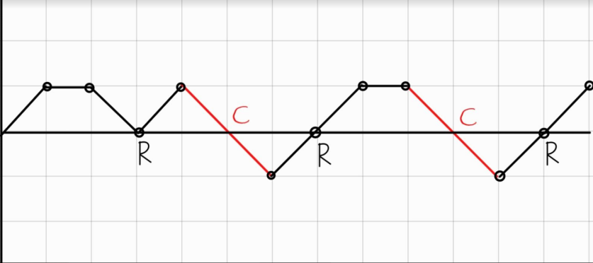
Figure 3: A directed random walk with 3 returns (R) to and 5 crossings (C) of the line $x=0$. The boundary local time = 8.

We end this discussion by illustrating the random walk behavior of the string in target spacetime and what boundary local time means in this case. As mentioned in the beginning of this section, the half-normal distribution emerges as the limit law for the local time at $x=0$ in directed lattice paths (random walks) on $\mathbb{Z}$ with no drift in the limit of large number of steps. Specifically,

$$\textrm{local time at zero = the number of returns to zero}+\text{number of }x\text{-axis crossings .}$$ (130)

The discrete nature of the boundary local time in directed random walks reveals the explicit random walk behavior of the string in target spacetime. In particular, the expectation value of the string nonzero mode can therefore, be understood as the average number of returns to the wall at zero. The larger this number is, the larger the average length of the string’s random walk at a given RG time ${\epsilon}^{-1}$.

5.4 Outlook and Future Directions

A generalization of the current work to $S^{1}/\mathbb{Z}_{2}$ and curved target spaces with boundaries is an interesting direction. The generalization to codimension-2 boundaries, especially conical geometries are all interesting future directions. A worldsheet understanding of how to impose Dirichlet boundary conditions on propagating fields in target spacetime is required to derive the GHY boundary term in the on-shell classical action. This, in turn, is important for deriving the classical black hole entropy GH .

A probabilistic understanding of the boundary local time in conical geometries may give us some clues that might help us unravel the nature of the boundary conditions required for a worldsheet derivation of the classical black hole entropy $\frac{A}{4G_{N}}$ and the Ryu-Takayanagi formula RTPhysRevLett.96.181602 as presented in LM2013 . In particular, figuring out the boundary local time in conical geometries near the tip of the cone may guide us to understand the boundary condition in the NLSM limit of the winding condensate Jafferis-ER=EPR:2021 ; Halder:2023adw . The authors of this article are now actively working on this direction.

In a forthcoming work GHYZihan , it will be shown that the metric total derivative terms for the metric obtained in Ahmadain:2022eso gives the GHY boundary term York:1972sj (more precisely the Einstein boundary term Einstein:1916cd ) in the classical action but with one-half the coefficient required to have a well-defined variational principle, if we assume Dirichlet boundary conditions. A proper worldsheet path integral calculation similar to the one in this work, but for Dirichlet boundary conditions, is therefore required to obtain the correct factor of “2” $\text{Tr}K$ and obtain a total action (EH plus GHY) with a well-defined variational principle.

Another very interesting direction involves understanding the behavior of strings at a finite non-asymptotic Dirichlet boundary on a bulk Cauchy slice in $\operatorname{AdS}$ Zamolodchikov:2004ce ; Smirnov:2016lqw ; Cavaglia:2016oda ; McGough:2016lol ; Araujo-Regado:2022gvw for T$\bar{\text{T}}$-deformed CFTs. The related question of placing a finite timelike boundary in an $\operatorname{AdS}$ black hole and in a $\operatorname{dS}$ static patch requires an understanding of the behavior of strings near totally absorbing walls with a Dirichlet boundary condition silverstein2023black ; Batra:2024kjl . It would be very interesting if the work in this paper can be generalized to address this question.

Appendix A The computation of $\left\langle\absolutevalue{Y^{D}+\sqrt{\alpha^{\prime}}\eta^{D}(z)}\right\rangle$

In this section we show how to compute the one-point function $\left\langle\absolutevalue{Y^{D}+\sqrt{\alpha^{\prime}}\eta^{D}(z)}\right\rangle$. Let us in fact be more general and compute $\left\langle f\left(\eta^{D}(z)\right)\right\rangle$ for an arbitrary function $f\left(\eta^{D}(z)\right)$.

The first step is to expand $\eta^{D}(z)$ in spherical harmonics

$$\eta^{D}(z)=\sum_{l=1}^{\infty}\sum_{m=-l}^{m=l}x_{lm}Y_{lm}(z),$$ (131)

where $Y_{lm}(z)$ are the real spherical hamonics

$$Y_{\ell m}=\begin{cases}\left(-1\right)^{m}\sqrt{2}\sqrt{\dfrac{2\ell+1}{4\pi}\dfrac{(\ell-|m|)!}{(\ell+|m|)!}}P_{\ell}^{|m|}(\cos\theta)\sin(|m|\varphi)&\text{if }m<0\\ \sqrt{\dfrac{2\ell+1}{4\pi}}P_{\ell}^{m}(\cos\theta)&\text{if }m=0\\ \left(-1\right)^{m}\sqrt{2}\sqrt{\dfrac{2\ell+1}{4\pi}\dfrac{(\ell-m)!}{(\ell+m)!}}P_{\ell}^{m}(\cos\theta)\cos(m\varphi)&\text{if }m>0\,.\end{cases}$$ (132)

They satisfy the Laplace equation in spherical coordinates

$$\nabla^{2}Y_{lm}(z)=-l(l+1)Y_{lm}(z)\,,$$ (133)

and are orthogonal

$$\int_{0}^{2\pi}d\phi\int_{0}^{\pi}d\theta\ \sin{\theta}\ Y_{lm}(\theta,\phi)Y_{l^{\prime}m^{\prime}}(\theta,\phi)=\delta_{ll^{\prime}}\delta_{mm^{\prime}}\,,$$ (134)

where $x_{lm}$ are the expansion coefficients, and the sum runs from $l=1$ to $\infty$, not including the zero mode. Now we have

$$\left\langle f\left(\eta^{D}(z)\right)\right\rangle =\frac{1}{Z_{\text{nz}}}\int[D\sqrt{\alpha^{\prime}}\eta]e^{-I_{\text{p}}[\eta,g]}f\left(\eta^{D}(z)\right)$$ (135)

$$=\frac{1}{Z^{(D)}_{\text{nz}}}\int[D\sqrt{\alpha^{\prime}}\eta^{D}]e^{-I^{(D)}_{\text{p}}[\eta^{D},g]}f\left(\eta^{D}(z)\right),$$ (136)

where in the second line, we used the fact that the Polyakov action factorises into a sum of two terms: a term containing $\eta^{D}$ and another term containing $\eta^{i}$. Now we multiply by $1$ and express $1$ as a Dirac delta function

$$\left\langle f\left(\eta^{D}(z)\right)\right\rangle =\frac{1}{Z^{(D)}_{\text{nz}}}\int[D\sqrt{\alpha^{\prime}}\eta^{D}]e^{-I^{(D)}_{\text{p}}[\eta^{D},g]}f\left(\eta^{D}(z)\right)1$$ (137)

$$=\frac{1}{Z^{(D)}_{\text{nz}}}\int[D\sqrt{\alpha^{\prime}}\eta^{D}]e^{-I^{(D)}_{\text{p}}[\eta^{D},g]}f\left(\eta^{D}(z)\right)\int_{-\infty}^{\infty}d\xi\ \delta\left(\xi-\eta^{D}(z)\right)$$ (138)

$$=\frac{1}{Z^{(D)}_{\text{nz}}}\int_{-\infty}^{\infty}d\xi\int[D\sqrt{\alpha^{\prime}}\eta^{D}]e^{-I^{(D)}_{\text{p}}[\eta^{D},g]}f\left(\sum_{l=1}^{\infty}\sum_{m=-l}^{m=l}x_{lm}Y_{lm}(z_{0})\right)\ \delta\left(\xi-\sum_{l=1}^{\infty}\sum_{m=-l}^{m=l}x_{lm}Y_{lm}(z)\right),$$ (139)

where the measure in terms of the expansion coefficients is now

$$[D\sqrt{\alpha^{\prime}}\eta^{D}]=\prod_{l=1}^{\infty}\prod_{m=-l}^{m=l}\sqrt{\alpha^{\prime}}dx_{lm}\,.$$ (140)

The Polyakov action of the $\eta^{D}(z_{0})$ is given by (using the round sphere worldsheet metric)

$$I^{(D)}_{\text{p}}[\eta^{D},g] =\frac{1}{4\pi\alpha^{\prime}}\int d^{2}z\sqrt{g}\left(\alpha^{\prime}g^{ab}\partial_{a}\eta^{D}\partial_{b}\eta^{D}\right)+2\Phi_{0}$$ (141)

$$=-\frac{1}{4\pi\alpha^{\prime}}\int d^{2}z\sqrt{g}\left(\alpha^{\prime}\eta^{D}\nabla^{2}\eta^{D}\right)+2\Phi_{0}\,.$$ (142)

The heat kernel-regularized $I^{(D)}_{\text{p}}[\eta^{D},g]$ is given by

$$I^{(D)}_{\text{p}}[\eta^{D},g] =-\frac{1}{4\pi}\int d^{2}z\sqrt{g}\left(\eta^{D}e^{-\epsilon\nabla^{2}}\nabla^{2}\eta^{D}\right)+2\Phi_{0}$$ (143)

$$=-\frac{1}{4\pi}\sum_{l=1}^{\infty}\sum_{m=-l}^{m=l}(-l(l+1))e^{\epsilon l(l+1)}x^{2}_{lm}+2\Phi_{0}.$$ (144)

Thus, $\left\langle f\left(\eta^{D}(z)\right)\right\rangle$ is now given by

$$\left\langle f\left(\eta^{D}(z)\right)\right\rangle =\frac{e^{-2\Phi_{0}}}{Z^{(D)}_{\text{nz}}}\int_{-\infty}^{\infty}d\xi\int\left(\prod_{l=1}^{\infty}\prod_{m=-l}^{m=l}\sqrt{\alpha^{\prime}}dx_{lm}\right)e^{-\frac{1}{4\pi}\sum_{l=1}^{\infty}\sum_{m=-l}^{m=l}l(l+1)e^{\epsilon l(l+1)}x^{2}_{lm}}$$ (145)

$$f\left(\sum_{l=1}^{\infty}\sum_{m=-l}^{m=l}x_{lm}Y_{lm}(z_{0})\right)\ \delta\left(\xi-\sum_{l=1}^{\infty}\sum_{m=-l}^{m=l}x_{lm}Y_{lm}(z_{0})\right).$$ (146)

Without loss of generality, we can take $z$ to be the north pole. This is because $\left\langle f\left(\eta^{D}(z)\right)\right\rangle$is independent of $z$ due to translation symmetry of the scalar field $\eta^{D}(z)$ on the worldsheet, which is not broken even off-shell. Thus, we can just evaluate it at $z=z_{0}=0$

$$\left\langle f\left(\eta^{D}(z_{0})\right)\right\rangle =\frac{e^{-2\Phi_{0}}}{Z^{(D)}_{\text{nz}}}\int_{-\infty}^{\infty}d\xi\int\left(\prod_{l=1}^{\infty}\prod_{m=-l}^{m=l}\sqrt{\alpha^{\prime}}dx_{lm}\right)e^{-\frac{1}{4\pi}\sum_{l=1}^{\infty}\sum_{m=-l}^{m=l}l(l+1)e^{\epsilon l(l+1)}x^{2}_{lm}}$$ (147)

$$f\left(\sum_{l=1}^{\infty}\sum_{m=-l}^{m=l}x_{lm}Y_{lm}(0)\right)\ \delta\left(\xi-\sum_{l=1}^{\infty}\sum_{m=-l}^{m=l}x_{lm}Y_{lm}(0)\right).$$ (148)

At the north pole ($z_{0}=0$), the spherical hamonics vanish unless $m=0$, i.e. $Y_{lm}(0)=0$ when $m\neq 0$. So we get

$$\left\langle f\left(\eta^{D}(z_{0})\right)\right\rangle =\frac{e^{-2\Phi_{0}}}{Z^{(D)}_{\text{nz}}}\int_{-\infty}^{\infty}d\xi\int\left(\prod_{l=1}^{\infty}\prod_{m=-l}^{m=l}\sqrt{\alpha^{\prime}}dx_{lm}\right)e^{-\frac{1}{4\pi}\sum_{l=1}^{\infty}\sum_{m=-l}^{m=l}l(l+1)e^{\epsilon l(l+1)}x^{2}_{lm}}$$ (149)

$$f\left(\sum_{l=1}^{\infty}x_{l0}Y_{l0}(0)\right)\ \delta\left(\xi-\sum_{l=1}^{\infty}x_{l0}Y_{l0}(0)\right).$$ (150)

The $m\neq 0$ terms of the above integral factorises out and cancels the corresponding part in $Z^{(D)}_{\text{nz}}$ and we obtain

$$\left\langle f\left(\eta^{D}(z_{0})\right)\right\rangle =\frac{e^{-2\Phi_{0}}}{Z^{(D)}_{\text{nz}(m\neq 0)}}\int_{-\infty}^{\infty}d\xi\int\left(\prod_{l=1}^{\infty}\sqrt{\alpha^{\prime}}dx_{l0}\right)e^{-\frac{1}{4\pi}\sum_{l=1}^{\infty}l(l+1)e^{\epsilon l(l+1)}x^{2}_{l0}}$$ (151)

$$f\left(\sum_{l=1}^{\infty}x_{l0}Y_{l0}(0)\right)\ \delta\left(\xi-\sum_{l=1}^{\infty}x_{l0}Y_{l0}(0)\right).$$ (152)

Also, we have $Y_{l0}(0)=\sqrt{\dfrac{2l+1}{4\pi}}=:\omega_{l}$. So we have

$$\left\langle f\left(\eta^{D}(z_{0})\right)\right\rangle =\frac{e^{-2\Phi_{0}}}{Z^{(D)}_{\text{nz}(m\neq 0)}}\int_{-\infty}^{\infty}d\xi\int\left(\prod_{l=1}^{\infty}\sqrt{\alpha^{\prime}}dx_{l}\right)e^{-\frac{1}{4\pi}\sum_{l=1}^{\infty}l(l+1)e^{\epsilon l(l+1)}x^{2}_{l}}$$ (153)

$$f\left(\sum_{l=1}^{\infty}\omega_{l}x_{l}\right)\ \delta\left(\xi-\sum_{l=1}^{\infty}\omega_{l}x_{l}\right),$$ (154)

where we have dropped the subscript $``0"$ from $x_{l0}$ and $Y_{l0}$. We can absorb $\omega_{l}$ into $x_{l}$ by a change of integration variable to get

$$\left\langle f\left(\eta^{D}(z_{0})\right)\right\rangle =\frac{e^{-2\Phi_{0}}}{Z^{(D)}_{\text{nz}(m\neq 0)}}\int_{-\infty}^{\infty}d\xi\int\left(\prod_{l=1}^{\infty}\frac{\sqrt{\alpha^{\prime}}}{\omega_{l}}dx_{l}\right)e^{-\frac{1}{4\pi}\sum_{l=1}^{\infty}\frac{l(l+1)}{\omega_{l}^{2}}e^{\epsilon l(l+1)}x^{2}_{l}}$$ (155)

$$f\left(\sum_{l=1}^{\infty}x_{l}\right)\ \delta\left(\xi-\sum_{l=1}^{\infty}x_{l}\right).$$ (156)

Now we shall pick a mode to integrate over, say $x_{1}$. Integrating over $x_{1}$, we obtain

$$\left\langle f\left(\eta^{D}(z_{0})\right)\right\rangle =\frac{\sqrt{\alpha^{\prime}}e^{-2\Phi_{0}}}{\omega_{1}Z^{(D)}_{\text{nz}(m\neq 0)}}\int_{-\infty}^{\infty}d\xi\ f\left(\xi\right)\int\left(\prod_{l=2}^{\infty}\frac{\sqrt{\alpha^{\prime}}}{\omega_{l}}dx_{l}\right)$$ (157)

$$\exp{{-\frac{1}{4\pi}\sum_{l=2}^{\infty}\frac{l(l+1)}{\omega^{2}_{l}}e^{\epsilon l(l+1)}x^{2}_{l}}-\frac{2}{4\pi\omega^{2}_{1}}e^{2\epsilon}\left(\xi-\sum_{l=2}^{\infty}x_{l}\right)^{2}}$$ (158)

$$=\frac{\sqrt{\alpha^{\prime}}e^{-2\Phi_{0}}}{\omega_{1}Z^{(D)}_{\text{nz}(m\neq 0)}}\int_{-\infty}^{\infty}d\xi\ f\left(\xi\right)e^{-\frac{2}{4\pi\omega^{2}_{1}}e^{2\epsilon}\xi^{2}}\int\left(\prod_{l=2}^{\infty}\frac{\sqrt{\alpha^{\prime}}}{\omega_{l}}dx_{l}\right)$$ (159)

$$\exp{-\frac{1}{4\pi}\sum_{l=2}^{\infty}\frac{l(l+1)}{\omega^{2}_{l}}e^{\epsilon l(l+1)}x^{2}_{l}-\frac{2}{4\pi\omega^{2}_{1}}e^{2\epsilon}\left(\sum_{l=2}^{\infty}x_{l}\right)^{2}-\frac{4}{4\pi\omega^{2}_{1}}e^{2\epsilon}\xi\sum_{l=2}^{\infty}x_{l}}$$ (160)

$$=\frac{\sqrt{\alpha^{\prime}}e^{-2\Phi_{0}}}{\omega_{1}Z^{(D)}_{\text{nz}(m\neq 0)}}\int_{-\infty}^{\infty}d\xi\ f\left(\xi\right)e^{-\frac{2}{4\pi\omega^{2}_{1}}e^{2\epsilon}\xi^{2}}\int\left(\prod_{l=2}^{\infty}\frac{\sqrt{\alpha^{\prime}}}{\omega_{l}}dx_{l}\right)e^{\Gamma},$$ (161)

where

$$\Gamma :=-\frac{1}{4\pi}\sum_{l=2}^{\infty}\frac{l(l+1)}{\omega^{2}_{l}}e^{\epsilon l(l+1)}x^{2}_{l}-\frac{2}{4\pi\omega^{2}_{1}}e^{2\epsilon}\left(\sum_{l=2}^{\infty}x_{l}\right)^{2}-\frac{4}{4\pi\omega^{2}_{1}}e^{2\epsilon}\xi\sum_{l=2}^{\infty}x_{l}$$ (162)

$$=-\frac{1}{4\pi}\sum_{n=2}^{\infty}\sum_{m=2}^{\infty}\frac{n(n+1)}{\omega^{2}_{n}}e^{\epsilon n(n+1)}x_{n}\delta_{nm}x_{m}-\frac{2}{4\pi\omega^{2}_{1}}e^{2\epsilon}\sum_{n=2}^{\infty}\sum_{m=2}^{\infty}x_{n}x_{m}-\frac{4}{4\pi\omega^{2}_{1}}e^{2\epsilon}\xi\sum_{l=2}^{\infty}x_{l}$$ (163)

$$=-\sum_{n=2}^{\infty}\sum_{m=2}^{\infty}\frac{1}{2\pi\omega^{2}_{1}}e^{2\epsilon}\left(\frac{\omega^{2}_{1}}{\omega^{2}_{n}}\frac{n(n+1)}{2}e^{\epsilon n(n+1)-2\epsilon}\delta_{nm}+1\right)x_{n}x_{m}-\frac{4}{4\pi\omega^{2}_{1}}e^{2\epsilon}\xi\sum_{l=2}^{\infty}x_{l}$$ (164)

$$=-M_{nm}\tilde{x}_{n}\tilde{x}_{m}-\frac{1}{\omega_{1}}\sqrt{\frac{2}{\pi}}e^{\epsilon}\xi\sum_{l=2}^{\infty}\tilde{x}_{l},$$ (165)

and

$$M_{nm} :=\left(\tilde{\lambda}_{n}\delta_{nm}+1\right)$$ (166)

$$\tilde{\lambda}_{n} :=\frac{\omega^{2}_{1}}{\omega^{2}_{n}}\frac{n(n+1)}{2}e^{\epsilon n(n+1)-2\epsilon}$$ (167)

$$\tilde{x}_{n} :=\frac{1}{\sqrt{2\pi}\omega_{1}}e^{\epsilon}x_{n}$$ (168)

So we get

$$\left\langle f\left(\eta^{D}(z_{0})\right)\right\rangle =\left(\prod_{l=2}^{\infty}\frac{\omega_{1}}{\omega_{l}}\right)\frac{\sqrt{\alpha^{\prime}}e^{-2\Phi_{0}}}{\omega_{1}Z^{(D)}_{\text{nz}(m\neq 0)}}\int_{-\infty}^{\infty}d\xi\ f\left(\xi\right)e^{-\frac{1}{2\pi\omega^{2}_{1}}e^{2\epsilon}\xi^{2}}\int\left(\prod_{l=2}^{\infty}\sqrt{2\pi\alpha^{\prime}}e^{-\epsilon}d\tilde{x}_{l}\right)e^{\Gamma},$$ (169)

Now let us diagonalise the real symmetric matrix M by an orthogonal transformation $\tilde{x}_{n}=\Lambda_{nm}y_{m}$ to get a diagonal matrix $D=\Lambda^{T}M\Lambda$

$$\left\langle f\left(\eta^{D}(z_{0})\right)\right\rangle =\left(\prod_{l=2}^{\infty}\frac{\omega_{1}}{\omega_{l}}\right)\frac{\sqrt{\alpha^{\prime}}e^{-2\Phi_{0}}}{\omega_{1}Z^{(D)}_{\text{nz}(m\neq 0)}}\int_{-\infty}^{\infty}d\xi\ f\left(\xi\right)e^{-\frac{1}{2\pi\omega^{2}_{1}}e^{2\epsilon}\xi^{2}}\frac{1}{\text{Det}(\Lambda)}\int\left(\prod_{n=2}^{\infty}\sqrt{2\pi\alpha^{\prime}}e^{-\epsilon}dy_{n}\right)$$ (170)

$$\exp{-\sum_{n=2}^{\infty}D_{n}y^{2}_{n}-\xi\sum_{n=2}^{\infty}k_{n}y_{n}},$$ (171)

where $k_{n}:=\frac{1}{\omega_{1}}\sum_{m=2}^{\infty}\sqrt{\frac{2}{\pi}}e^{\epsilon}\Lambda_{mn}$ and a factor of $\text{Det}(\Lambda)$ comes from the Jacobian. Now one can complete the squares and shift the mean to get (one can check that all $D_{n}>0$)

$$\left\langle f\left(\eta^{D}(z_{0})\right)\right\rangle =\left(\prod_{l=2}^{\infty}\frac{\omega_{1}}{\omega_{l}}\right)\frac{\sqrt{\alpha^{\prime}}e^{-2\Phi_{0}}}{\omega_{1}Z^{(D)}_{\text{nz}(m\neq 0)}}\int_{-\infty}^{\infty}d\xi\ f\left(\xi\right)e^{-\frac{1}{2\pi\omega^{2}_{1}}e^{2\epsilon}\xi^{2}}\frac{1}{\text{Det}(\Lambda)}\exp{\sum_{n=2}^{\infty}\frac{k^{2}_{n}}{4D_{n}}\xi^{2}}$$ (172)

$$\prod_{n=2}^{\infty}\int\sqrt{2\pi\alpha^{\prime}}e^{-\epsilon}dy_{n}\exp{-D_{n}\left(y_{n}+\xi\frac{k_{n}}{2D_{n}}\right)^{2}}$$ (173)

$$=\left(\prod_{l=2}^{\infty}\frac{\omega_{1}}{\omega_{l}}\right)\frac{\sqrt{\alpha^{\prime}}e^{-2\Phi_{0}}}{\omega_{1}Z^{(D)}_{\text{nz}(m\neq 0)}}\frac{1}{\text{Det}(\Lambda)}\frac{1}{\sqrt{\text{Det}(M)}}\left(\prod_{n=2}^{\infty}\sqrt{2\alpha^{\prime}}\pi e^{-\epsilon}\right)$$ (174)

$$\int_{-\infty}^{\infty}d\xi\ f\left(\xi\right)e^{-\frac{1}{2\pi\omega^{2}_{1}}e^{2\epsilon}\xi^{2}}\exp{\sum_{n=2}^{\infty}\frac{k^{2}_{n}}{4D_{n}}\xi^{2}}.$$ (175)

All of the annoying factors in (174) gets absorbed into $Z^{(D)}_{\text{nz}(m\neq 0)}$ and we finaly get

$$\left\langle f\left(\eta^{D}(z_{0})\right)\right\rangle =\frac{\int_{-\infty}^{\infty}d\xi\ f\left(\xi\right)e^{-\xi^{2}/\Omega}}{\int_{-\infty}^{\infty}d\xi\ e^{-\xi^{2}/\Omega}},$$ (176)

where

$$\Omega^{-1} :=\frac{e^{2\epsilon}}{2\pi\omega^{2}_{1}}\left(1-\mathbb{M}\right)\,,$$ (177)

$$\mathbb{M} :=\omega^{2}_{1}\frac{\pi}{2}e^{-2\epsilon}\sum_{n=2}^{\infty}\frac{k^{2}_{n}}{D_{n}}\,.$$ (178)

Now let us calculate $\mathbb{M}$.

$$\mathbb{M} =\omega^{2}_{1}\frac{\pi}{2}e^{-2\epsilon}\sum_{n=2}^{\infty}\frac{k^{2}_{n}}{D_{n}}=\frac{\pi}{2}e^{-2\epsilon}\sum_{n=2}^{\infty}\sum_{m=2}^{\infty}\sum_{\tilde{m}=2}^{\infty}\sqrt{\frac{2}{\pi}}e^{\epsilon}\Lambda_{mn}\frac{1}{D_{n}}\sqrt{\frac{2}{\pi}}e^{\epsilon}\Lambda_{\tilde{m}n}$$ (179)

$$=\sum_{n=2}^{\infty}\sum_{m=2}^{\infty}[\Lambda D^{-1}\Lambda^{T}]_{nm}=\sum_{n=2}^{\infty}\sum_{m=2}^{\infty}[M^{-1}]_{nm},$$ (180)

which follows from $\Lambda$ being an orthogonal matrix. So $\mathbb{M}$ is the sum of all the entries of the inverse of the matrix $M$. One can show that

$$\mathbb{M}=\frac{1}{1+\frac{1}{\sum_{n=2}^{\infty}\tilde{\lambda}_{n}^{-1}}}\,\,.$$ (181)

One can also show that

$$\Omega=\left(\frac{e^{2\epsilon}}{2\pi\omega^{2}_{1}}\left(1-\mathbb{M}\right)\right)^{-1} =\frac{2\pi\omega^{2}_{1}}{e^{2\epsilon}}\left(1+\sum_{n=2}^{\infty}\tilde{\lambda}_{n}^{-1}\right)=\frac{3}{2}e^{-2\epsilon}+\sum_{n=2}^{\infty}\frac{2n+1}{n(n+1)}e^{-\epsilon n(n+1)}$$ (182)

$$=\sum_{n=1}^{\infty}\frac{2n+1}{n(n+1)}e^{-\epsilon n(n+1)}\,.$$ (183)

If we specialize to $f\left(\eta^{D}(z_{0})\right)=\absolutevalue{\eta^{D}(z_{0})}^{N}$, then the general formula in equation (176) reduces to

$$\left\langle\absolutevalue{\eta^{D}(z_{0})}^{N}\right\rangle =\frac{\int_{-\infty}^{\infty}d\xi\ \absolutevalue{\xi}^{N}e^{-\xi^{2}/\Omega}}{\int_{-\infty}^{\infty}d\xi\ e^{-\xi^{2}/\Omega}}=\frac{\int_{0}^{\infty}d\xi\ \xi^{N}e^{-\xi^{2}/\Omega}}{\int_{0}^{\infty}d\xi\ e^{-\xi^{2}/\Omega}}$$ (184)

$$=\frac{1}{\sqrt{\pi}}\Gamma\left(\frac{1+N}{2}\right)\Omega^{N/2}.$$ (185)

We thus get

$$\left\langle\absolutevalue{\eta^{D}(z_{0})}^{N}\right\rangle =\frac{1}{\sqrt{\pi}}\Gamma\left(\frac{1+N}{2}\right)\left(\sum_{n=1}^{\infty}\frac{2n+1}{n(n+1)}e^{-\epsilon n(n+1)}\right)^{N/2}\,.$$ (186)

The $N=2$ case is a standard result, so we shall compare our result with it. We know that Andreev:1990iv

$$\left\langle\eta^{\mu}(z)\eta^{\nu}\left(z\right)\right\rangle =2\pi\alpha^{\prime}\delta^{\mu\nu}\left(\frac{1}{4\pi}\sum_{n=1}^{\infty}\frac{2n+1}{n(n+1)}e^{-\epsilon n(n+1)}\right)$$

$$=2\pi\alpha^{\prime}\delta^{\mu\nu}\left(-\frac{1}{2\pi}\alpha^{\prime}\log{\epsilon}+O({\epsilon}^{2})+\text{finite term}\right)\,.$$

Thus, we find from (182) that $\Omega=2\log{\epsilon}^{-1}$.

Now we focus on the original term we set out to compute: $\left\langle\absolutevalue{Y^{D}+\sqrt{\alpha^{\prime}}\eta^{D}(z_{0})}\right\rangle$. For this, the general formula in equation (176) reduces to

$$\left\langle\absolutevalue{Y^{D}+\sqrt{\alpha^{\prime}}\eta^{D}(z_{0})}\right\rangle =\frac{\int_{-\infty}^{\infty}d\xi\ \absolutevalue{Y^{D}+\sqrt{\alpha^{\prime}}\xi}e^{-\xi^{2}/\Omega}}{\int_{-\infty}^{\infty}d\xi\ e^{-\xi^{2}/\Omega}}=\frac{1}{\sqrt{\pi\Omega}}\int_{-\infty}^{\infty}d\xi\ \absolutevalue{Y^{D}+\sqrt{\alpha^{\prime}}\xi}e^{-\xi^{2}/\Omega}$$ (187)

$$=\frac{1}{\sqrt{\pi\Omega}}\int_{-\frac{Y^{D}}{\sqrt{\alpha^{\prime}}}}^{\infty}d\xi\ \left(Y^{D}+\sqrt{\alpha^{\prime}}\xi\right)e^{-\xi^{2}/\Omega}-\frac{1}{\sqrt{\pi\Omega}}\int_{-\infty}^{-\frac{Y^{D}}{\sqrt{\alpha^{\prime}}}}d\xi\ \left(Y^{D}+\sqrt{\alpha^{\prime}}\xi\right)e^{-\xi^{2}/\Omega}$$ (188)

$$=\frac{Y^{D}}{\sqrt{\pi\Omega}}\int_{-\frac{Y^{D}}{\sqrt{\alpha^{\prime}}}}^{\infty}d\xi\ e^{-\xi^{2}/\Omega}-\frac{Y^{D}}{\sqrt{\pi\Omega}}\int_{-\infty}^{-\frac{Y^{D}}{\sqrt{\alpha^{\prime}}}}d\xi\ e^{-\xi^{2}/\Omega}$$ (189)

$$+\frac{\sqrt{\alpha^{\prime}}}{\sqrt{\pi\Omega}}\int_{-\frac{Y^{D}}{\sqrt{\alpha^{\prime}}}}^{\infty}d\xi\ \xi e^{-\xi^{2}/\Omega}-\frac{\sqrt{\alpha^{\prime}}}{\sqrt{\pi\Omega}}\int_{-\infty}^{-\frac{Y^{D}}{\sqrt{\alpha^{\prime}}}}d\xi\ \xi e^{-\xi^{2}/\Omega}$$ (190)

$$=\frac{Y^{D}}{\sqrt{\pi\Omega}}\frac{\sqrt{\pi\Omega}}{2}\left(1+\text{erf}\left(\frac{Y^{D}}{\sqrt{\alpha^{\prime}\Omega}}\right)\right)-\frac{Y^{D}}{\sqrt{\pi\Omega}}\frac{\sqrt{\pi\Omega}}{2}\left(\text{erfc}\left(\frac{Y^{D}}{\sqrt{\alpha^{\prime}\Omega}}\right)\right)$$ (191)

$$+\frac{\sqrt{\alpha^{\prime}}}{\sqrt{\pi\Omega}}\frac{\Omega}{2}e^{-\frac{(Y^{D})^{2}}{\alpha^{\prime}\Omega}}+\frac{\sqrt{\alpha^{\prime}}}{\sqrt{\pi\Omega}}\frac{\Omega}{2}e^{-\frac{(Y^{D})^{2}}{\alpha^{\prime}\Omega}}$$ (192)

$$=\sqrt{\Omega}\frac{\sqrt{\alpha^{\prime}}}{\sqrt{\pi}}e^{-\frac{(Y^{D})^{2}}{\alpha^{\prime}\Omega}}+\frac{Y^{D}}{2}\left(1+\text{erf}\left(\frac{Y^{D}}{\sqrt{\alpha^{\prime}\Omega}}\right)-\text{erfc}\left(\frac{Y^{D}}{\sqrt{\alpha^{\prime}\Omega}}\right)\right)$$ (193)

$$=\sqrt{\Omega}\frac{\sqrt{\alpha^{\prime}}}{\sqrt{\pi}}e^{-\frac{(Y^{D})^{2}}{\alpha^{\prime}\Omega}}+Y^{D}\text{erf}\left(\frac{Y^{D}}{\sqrt{\alpha^{\prime}\Omega}}\right).$$ (194)

So finally, we obtain our desired expression

$$\left\langle\absolutevalue{Y^{D}+\sqrt{\alpha^{\prime}}\eta^{D}(z_{0})}\right\rangle =\sqrt{\alpha^{\prime}}\left(\frac{\sqrt{\Omega}}{\sqrt{\pi}}e^{-\frac{(Y^{D})^{2}}{\alpha^{\prime}\Omega}}+\frac{Y^{D}}{\sqrt{\alpha^{\prime}}}\text{erf}\left(\frac{Y^{D}}{\sqrt{\alpha^{\prime}\Omega}}\right)\right)$$ (195)

$$=\sqrt{\alpha^{\prime}}\left(\left\langle\absolutevalue{\eta^{D}(z_{0})}\right\rangle e^{-\frac{(Y^{D})^{2}}{\alpha^{\prime}\Omega}}+\frac{Y^{D}}{\sqrt{\alpha^{\prime}}}\text{erf}\left(\frac{Y^{D}}{\sqrt{\alpha^{\prime}\Omega}}\right)\right).$$ (196)

where we used (184) in the last line that $\left\langle\absolutevalue{\eta^{D}(z_{0})}\right\rangle=\frac{\sqrt{\Omega}}{\sqrt{\pi}}$.

References

- (1) V.A. Kazakov and A.A. Tseytlin, On free energy of 2-D black hole in bosonic string theory, JHEP 06 (2001) 021 [hep-th/0104138].
- (2) A.A. Tseytlin, Partition Function of String Model on a Compact Two Space, Phys. Lett. B 223 (1989) 165.
- (3) O.D. Andreev, R.R. Metsaev and A.A. Tseytlin, Covariant calculation of the statistical sum of the two-dimensional sigma model on compact two surfaces., Sov. J. Nucl. Phys. 51 (1990) 359 [2301.02867].
- (4) A. Ahmadain and A.C. Wall, Off-Shell Strings II: Black Hole Entropy, 2211.16448.
- (5) A.A. Tseytlin, Mobius Infinity Subtraction and Effective Action in Model Approach to Closed String Theory, Phys. Lett. B 208 (1988) 221.
- (6) A. Ahmadain and A.C. Wall, Off-Shell Strings I: S-matrix and Action, 2211.08607.
- (7) H. Erbin, String Field Theory: A Modern Introduction, vol. 980 of Lecture Notes in Physics (3, 2021), 10.1007/978-3-030-65321-7.
- (8) J. Liu and J. Polchinski, Renormalization of the Mobius Volume, Phys. Lett. B 203 (1988) 39.
- (9) E.S. Fradkin and A.A. Tseytlin, Quantum String Theory Effective Action, Nucl. Phys. B 261 (1985) 1. [Erratum: Nucl.Phys.B 269, 745–745 (1986)].
- (10) E.S. Fradkin and A.A. Tseytlin, Effective Field Theory from Quantized Strings, Phys. Lett. B 158 (1985) 316.
- (11) E.S. Fradkin and A.A. Tseytlin, Effective Action Approach to Superstring Theory, Phys. Lett. B 160 (1985) 69.
- (12) A.A. Tseytlin, Tachyon effective actions in string theory, Theor. Math. Phys. 128 (2001) 1293.
- (13) A. Adams, J. Polchinski and E. Silverstein, Don’t panic! Closed string tachyons in ALE space-times, JHEP 10 (2001) 029 [hep-th/0108075].
- (14) L. Eberhardt and S. Pal, Holographic Weyl anomaly in string theory, SciPost Phys. 16 (2024) 027 [2307.03000].
- (15) A.A. Tseytlin, Sigma model approach to string theory effective actions with tachyons, J. Math. Phys. 42 (2001) 2854 [hep-th/0011033].
- (16) A.A. Tseytlin, On sigma model RG flow, ’central charge’ action and Perelman’s entropy, Phys. Rev. D 75 (2007) 064024 [hep-th/0612296].
- (17) P. Kraus, A. Ryzhov and M. Shigemori, Strings in noncompact space-times: Boundary terms and conserved charges, Phys. Rev. D 66 (2002) 106001 [hep-th/0206080].
- (18) T. Erler, The closed string field theory action vanishes, JHEP 10 (2022) 055 [2204.12863].
- (19) A. Sen and B. Zwiebach, String Field Theory: A Review, 2405.19421.
- (20) Y. Chen, J. Maldacena and E. Witten, On the black hole/string transition, Journal of High Energy Physics 2023 (2023) 1.
- (21) T. Erler, The closed string field theory action vanishes, 2204.12863.
- (22) J. Troost, The ads3 central charge in string theory, Physics Letters B 705 (2011) 260.
- (23) J.W. York, Jr., Role of conformal three geometry in the dynamics of gravitation, Phys. Rev. Lett. 28 (1972) 1082.
- (24) G.W. Gibbons and S.W. Hawking, Action Integrals and Partition Functions in Quantum Gravity, Phys. Rev. D 15 (1977) 2752.
- (25) L. Eberhardt and S. Pal, The disk partition function in string theory, JHEP 08 (2021) 026 [2105.08726].
- (26) R. Mahajan, D. Stanford and C. Yan, Sphere and disk partition functions in Liouville and in matrix integrals, JHEP 07 (2022) 132 [2107.01172].
- (27) B. Mühlmann, The two-sphere partition function in two-dimensional quantum gravity at fixed area, JHEP 09 (2021) 189 [2106.04532].
- (28) L. Eberhardt and S. Pal, Holographic weyl anomaly in string theory, arXiv preprint arXiv:2307.03000 (2023) .
- (29) T.G. Mertens, Hagedorn String Thermodynamics in Curved Spacetimes and near Black Hole Horizons, Ph.D. thesis, Gent U., 2015. 1506.07798.
- (30) F. Bastianelli, O. Corradini and P.A.G. Pisani, Worldline approach to quantum field theories on flat manifolds with boundaries, JHEP 02 (2007) 059 [hep-th/0612236].
- (31) F. Bastianelli, O. Corradini, P.A.G. Pisani and C. Schubert, Scalar heat kernel with boundary in the worldline formalism, JHEP 10 (2008) 095 [0809.0652].
- (32) F. Bastianelli, O. Corradini, P.A.G. Pisani and C. Schubert, Worldline Approach to QFT on Manifolds with Boundary, in 9th Conference on Quantum Field Theory under the Influence of External Conditions (QFEXT 09): Devoted to the Centenary of H. B. G. Casimir, pp. 415–420, 2010, DOI [0912.4120].
- (33) E.W. Weisstein, “Half-normal distribution.” from mathworld–a wolfram web resource.” https://mathworld.wolfram.com/Half-NormalDistribution.html.
- (34) P. Mörters and Y. Peres, Brownian motion, vol. 30, Cambridge University Press (2010).
- (35) I. Karatzas and S. Shreve, Brownian motion and stochastic calculus, vol. 113, springer (2014).
- (36) P. Lévy, Processus stochastiques et mouvement brownien (paris: Gauthier-villars) google scholar lévy p 1951, in Proc. 2nd Berkeley Symp. on Mathematical Statistics and Probability, 1965.
- (37) K. Ito and H. McKean, Diffusion processes and their sample paths, Die Grundlehren der Mathematischen Wissenschaften in Einzeldarstellungen 125 (1965) .
- (38) P.-L. Lions and A.-S. Sznitman, Stochastic differential equations with reflecting boundary conditions, Communications on pure and applied Mathematics 37 (1984) 511.
- (39) Y. Saisho, Stochastic differential equations for multi-dimensional domain with reflecting boundary, Probability Theory and Related Fields 74 (1987) 455.
- (40) P. Hsu, Probabilistic approach to the neumann problem, Communications on pure and applied mathematics 38 (1985) 445.
- (41) A.N. Borodin and P. Salminen, Handbook of Brownian motion-facts and formulae, Springer Science & Business Media (2015).
- (42) D.S. Grebenkov, Probability distribution of the boundary local time of reflected brownian motion in euclidean domains, Physical Review E 100 (2019) 062110.
- (43) K. Siegrist, “Probability, mathematical statistics, stochastic processes.” https://www.randomservices.org/random/special/FoldedNormal.html/.
- (44) C. Banderier and M. Wallner, Local time for lattice paths and the associated limit laws, arXiv preprint arXiv:1805.09065 (2018) .
- (45) M. Wallner, A half-normal distribution scheme for generating functions, European Journal of Combinatorics 87 (2020) 103138.
- (46) A.V. Skorokhod, Stochastic equations for diffusion processes in a bounded region, Theory of Probability & Its Applications 6 (1961) 264.
- (47) A.V. Skorokhod, Stochastic equations for diffusion processes in a bounded region. ii, Theory of Probability & Its Applications 7 (1962) 3.
- (48) H. Tanaka, Stochastic differential equations with reflecting, Stochastic Processes: Selected Papers of Hiroshi Tanaka 9 (1979) 157.
- (49) K.L. Chung, Z. Zhao, K.L. Chung and Z. Zhao, Killed brownian motion, From Brownian Motion to Schrödinger’s Equation (1995) 31.
- (50) T. Björk, The pedestrian’s guide to local time, 1512.08912.
- (51) H.P. McKean, Stochastic integrals, vol. 353, American Mathematical Soc. (1969).
- (52) T.E. Clark, R. Menikoff and D.H. Sharp, Quantum mechanics on the half-line using path integrals, Phys. Rev. D 22 (1980) 3012.
- (53) L. Takács, On the local time of the brownian motion, The Annals of Applied Probability (1995) 741.
- (54) G.W. Gibbons and S.W. Hawking, Action integrals and partition functions in quantum gravity, Phys. Rev. D 15 (1977) 2752.
- (55) S. Ryu and T. Takayanagi, Holographic derivation of entanglement entropy from the anti–de sitter space/conformal field theory correspondence, Phys. Rev. Lett. 96 (2006) 181602.
- (56) A. Lewkowycz and J. Maldacena, Generalized gravitational entropy, JHEP 08 (2013) 090 [1304.4926].
- (57) D.L. Jafferis and E. Schneider, Stringy ER=EPR, 2104.07233.
- (58) I. Halder and D.L. Jafferis, Thermal Bekenstein-Hawking entropy from the worldsheet, 2310.02313.
- (59) A. Ahmadain, V. Shyam and Y. Zihan, One-half the Einstein boundary term from the string worldsheet, forthcoming, .
- (60) A. Einstein, Hamilton’s Principle and the General Theory of Relativity, Sitzungsber. Preuss. Akad. Wiss. Berlin (Math. Phys. ) 1916 (1916) 1111.
- (61) A.B. Zamolodchikov, Expectation value of composite field T anti-T in two-dimensional quantum field theory, hep-th/0401146.
- (62) F.A. Smirnov and A.B. Zamolodchikov, On space of integrable quantum field theories, Nucl. Phys. B 915 (2017) 363 [1608.05499].
- (63) A. Cavaglià, S. Negro, I.M. Szécsényi and R. Tateo, -deformed 2D Quantum Field Theories, JHEP 10 (2016) 112 [1608.05534].
- (64) L. McGough, M. Mezei and H. Verlinde, Moving the CFT into the bulk with , JHEP 04 (2018) 010 [1611.03470].
- (65) G. Araujo-Regado, R. Khan and A.C. Wall, Cauchy slice holography: a new AdS/CFT dictionary, JHEP 03 (2023) 026 [2204.00591].
- (66) E. Silverstein, Black hole to cosmic horizon microstates in string/m theory: timelike boundaries and internal averaging, Journal of High Energy Physics 2023 (2023) 1 [2212.00588].
- (67) G. Batra, G.B. De Luca, E. Silverstein, G. Torroba and S. Yang, Bulk-local dS3 holography: the Matter with , 2403.01040.