Profiled Transfer Learning for High Dimensional Linear Model

Abstract

We develop here a novel transfer learning methodology called Profiled Transfer Learning (PTL). The method is based on the approximate-linear assumption between the source and target parameters. Compared with the commonly assumed vanishing-difference assumption and low-rank assumption in the literature, the approximate-linear assumption is more flexible and less stringent. Specifically, the PTL estimator is constructed by two major steps. Firstly, we regress the response on the transferred feature, leading to the profiled responses. Subsequently, we learn the regression relationship between profiled responses and the covariates on the target data. The final estimator is then assembled based on the approximate-linear relationship. To theoretically support the PTL estimator, we derive the non-asymptotic upper bound and minimax lower bound. We find that the PTL estimator is minimax optimal under appropriate regularity conditions. Extensive simulation studies are presented to demonstrate the finite sample performance of the new method. A real data example about sentence prediction is also presented with very encouraging results.

KEYWORDS: Approximate Linear Assumption; High Dimensional Data; High Dimensional Linear Regression; Profiled Transfer Learning; Transfer Learning

1. INTRODUCTION

High dimensional data have commonly emerged in many applications (Deng et al., 2009; Fan et al., 2020). However, one often has very limited sample sizes due to various practical reasons such as the ethical issues, data collection costs, and possibly others (Lee and Yoon, 2017; Wang et al., 2020). Consider for example a lung cancer dataset featured in the work by Zhou et al. (2023). In this study, 3D computed tomography (CT) images with unified voxel sizes of approximately $60\times 60\times 60$ were collected for each patient. The objective there was to diagnose the nodule type being benign or malignant. However, the cost for diagnosing nodule type is notably high and the sample size can hardly be large. In the study of Zhou et al. (2023), only a total of 1,075 subjects were collected. Taking into account the covariates (i.e. CT images) being of size about $60\times 60\times 60$, the sample size of 1,075 is exceedingly small. Similar issues can also be found in numerous other disciplines, including marketing (Wang, 2009), computer vision (Vinyals et al., 2016; Bateni et al., 2020), and natural language processing (Mcauliffe and Blei, 2007).

It is well known that sample sizes play a fundamental role in statistical modeling, determining the accuracy of estimators or powers of test statistics. Small sample sizes raise serious challenges for high dimensional data analysis. One way to address this problem is to impose some low-dimensional structures on the high-dimensional model of interest. For example, when high dimensional linear model are concerned, it is commonly assumed that the parameters are sparse, resulting in variously shrinkage estimation methods such as LASSO, SCAD, MCP and many others (Tibshirani, 1996; Fan and Li, 2001; Zou and Hastie, 2005; Yuan and Lin, 2006; Zou, 2006; Wang and Leng, 2007; Zhang, 2010) and feature screening methods (Fan and Lv, 2008; Wang, 2009; Fan and Song, 2010; Zhu et al., 2011; Li et al., 2012, etc.). Another commonly used approach is to assume some (approximately) low rank structures. For example, reduced rank regression assumes a low-rank coefficient matrix (Anderson, 1951; Izenman, 1975; Anderson, 1999; Chen and Huang, 2012; Reinsel et al., 2022), while factor model assumes the covariance matrix is approximately low rank (Bai and Ng, 2002; Stock and Watson, 2002; Bai, 2003; Fan et al., 2008; Bai and Li, 2012; Lam and Yao, 2012; Wang, 2012). However, these assumptions may be violated. Consider for example a study exploring the effect of single-nucleotide polymorphisms (SNPs) on height, as reported by Boyle et al. (2017). In this study, the total sample size amounts to 253,288 with a feature dimension of approximately 10 million. Moreover, this study suggests that there are about 400,000 common SNPs potentially having nonzero causal effects on height. Consequently, the associated regression coefficient vector is not too sparse. Recently estimations of nonsparse parameters have been also considered (Azriel and Schwartzman, 2020; Silin and Fan, 2022; Zhao et al., 2023b). Similarly the low dimensional structure is hard to verify and may be violated in practice.

To solve the problem, a number of researchers have advocated the idea of transfer learning (Pan and Yang, 2009; Weiss et al., 2016). For convenience, the dataset associated with the problem at hand is referred to as the target dataset. The main idea of transfer learning is to borrow strengths from some auxiliary datasets that will be referred to as source datasets. The parameters associated with sources and the target are termed the source parameters and the target parameters, respectively. To borrow strengths from source datasets, certain types of assumptions have to be imposed on the similarity between the target and source datasets. For example, Li et al. (2022) and Zhao et al. (2023a) considered transfer learning of high dimensional linear model, assuming that the $\ell_{q}$-distance ($0\leq q\leq 1$) between the target parameter and some of the source parameters should be sufficiently small. For convenience, we refer to this assumption as the vanishing-difference assumption. Similar assumption was also used by Tian and Feng (2022) and Li et al. (2023) for generalized linear models, Lin and Reimherr (2022) for functional linear regression, and Cai and Pu (2022) for nonparametric regression. As an alternative approach, Du et al. (2020) and Tripuraneni et al. (2021) assumed the source parameters and the target parameter can be linearly approximated by a common set of vectors in a low-dimensional subspace. We refer to this as the low-rank assumption. When these assumptions are satisfied, it has been shown that statistical efficiency can be enhanced significantly in these works.

Despite the success of the transfer learning methods, the similarity assumptions of these methods (i.e. the vanishing-difference assumption and the low-rank assumption) are stringent. For example, according to the vanishing-difference assumption, only those source datasets with parameters very close to the target one can be used for transfer learning, making the task of detecting transferable source datasets extremely crucial (Tian and Feng, 2022). On the other hand, the low-rank assumption is not perfect either. In practice, situations often arise where the parameters associated with the target and various sources are linearly independent, making it challenging to identify a low rank structure for the linear subspace spanned by these parameters. Even if the low-rank assumption holds, how to practically determine the structural dimension with finite data remains an additional challenging issue (Bai and Ng, 2002; Luo et al., 2009; Lam and Yao, 2012).

In this paper, we focus on transfer learning for high dimensional linear models. To implement transfer learning with less stringent similarity assumptions, we propose here a novel method named Profiled Transfer Learning (PTL). Our approach assumes that the target parameter can be linearly approximated by the source parameters without the stringent rank constraint. Specifically, we assume that there are $K$ sources, and consider high dimensional linear models for both target and sources. Denote parameter of the target model as $\bm{\beta}\in\mathbb{R}^{p}$, and the parameter of source $k$ as $\bm{\beta}^{(k)}\in\mathbb{R}^{p}$, for $k=1,\dots,K$. Then we assume that $\bm{\beta}=\sum_{k=1}^{K}w_{k}\bm{\beta}^{(k)}+\bm{\delta}$ for some constants $w_{k}$’s and $\bm{\delta}\in\mathbb{R}^{p}$. This assumption is referred to as approximate-linear assumption. Unlike the vanishing-difference assumption, approximate-linear assumption allows the difference between the target and source parameters (i.e. $\|\bm{\beta}^{(k)}-\bm{\beta}\|_{q}$) to be arbitrarily large. Additionally, different from the low-rank assumption, the approximate-linear assumption allows the structural dimension of the subspace spanned be $\bm{\beta}^{(k)}$’s to be as large as $K$.

Based on the approximate-linear assumption, we propose here a profiled transfer learning method with two major steps. Let $Y\in\mathbb{R}$ and $X\in\mathbb{R}^{p}$ be the response and covariates for the target linear model, respectively. In the first step, we estimate $\widehat{\bm{\beta}}^{(k)}$ using data from source $k$ to generate the transferred features $\widehat{Z}=\widehat{B}^{\top}X$ in the target data, where $\widehat{B}=(\widehat{\bm{\beta}}^{(k)},k=1,\dots,K)\in\mathbb{R}^{p\times K}$. Then we regress the response $Y$ on the transferred features $\widehat{Z}$ using the target data, treating the resulting residuals as the profiled responses. In the second step, the regression relationship between the profiled responses and the covariates $X$ is learned by some sparse learning method (e.g. LASSO) on the target data. Then the final estimator for the target parameter is assembled. Theoretical and numerical analyses suggest that our estimator can significantly improve the statistical efficiency, even in scenarios where both the vanishing-difference and the low-rank assumptions are violated.

The remainder of the paper is organized as follows. In Section 2, we introduce the profiled transfer learning method. The non-asymptotic upper bound and the minimax lower bound are presented in Section 3. Simulation experiments and real data analysis are reported in Section 4. We conclude the paper by a brief discussion about future researches in Section 5. All the technical details are provided in the Appendix.

Notations. For any vector $\bm{v}=(v_{1},\dots,v_{p})^{\top}\in\mathbb{R}^{p}$, denote $\|\bm{v}\|_{1}$, $\|\bm{v}\|$ and $\|\bm{v}\|_{\infty}$ as its $\ell_{1}$, $\ell_{2}$ and $\ell_{\infty}$ norms, respectively; denote $\|\bm{v}\|_{0}=\sum_{j=1}^{p}I(v_{j}\neq 0)$ as the $\ell_{0}$ norm of $\bm{v}$ and $\mbox{supp}(\bm{v})=\{i:v_{j}\neq 0,j=1,\dots,p\}$ as the associated support set. Define $\lambda_{\max}(A)$ and $\lambda_{\min}(A)$ to be the maximum and minimum eigenvalues for an arbitrary symmetric matrix $A\in\mathbb{R}^{p\times p}$. For any $A\in\mathbb{R}^{p_{1}\times p_{2}}$, we define its operator norm as $\|A\|_{\text{op}}=\sqrt{\lambda_{\max}(A^{\top}A)}$ and Frobenius norm as $\|A\|_{F}=\sqrt{\mbox{tr}(A^{\top}A)}$, respectively. For a sub-Gaussian random variable $U\in\mathbb{R}$, define its sub-Gaussian norm to be $\|U\|_{\psi_{2}}=\inf\{t>0:E\exp(U^{2}/t^{2})\leq 2\}$. For a sub-Gaussian random vector $V$, define its sub-Gaussian norm to be $\|V\|_{\psi_{2}}=\sup_{\|u\|=1}\|u^{\top}V\|_{\psi_{2}}$. Let $a\wedge b=\min\{a,b\}$ and $a\vee b=\max\{a,b\}$ for any real $a,b\in\mathbb{R}$. Write $a\lesssim b$ if there exists a constant $C>0$ such that $a\leq Cb$.

2. PROFILED TRANSFER LEARNING FOR HIGH DIMENSIONAL LINEAR MODEL

2.1. Target and Source Models

Similar to Li et al. (2022), we consider linear regression models for both target and sources in this paper. Let $\{(Y_{i},X_{i}),i=1,\dots,n\}$ be i.i.d. observations from the following target model

$$Y_{i}=X_{i}^{\top}\bm{\beta}+\varepsilon_{i},\qquad i=1,\cdots,n,$$ (2.1)

where $Y_{i}\in\mathbb{R}$ denotes the response and $X_{i}=(X_{i1},\dots,X_{ip})^{\top}\in\mathbb{R}^{p}$ denotes the associated $p$-dimensional covariates, satisfying $E(X_{i})=0$. Denote the covariance matrix of $X_{i}$ as $\Sigma=\mbox{cov}(X_{i})$. In addition, $\bm{\beta}=(\beta_{1},\dots,\beta_{p})^{\top}\in\mathbb{R}^{p}$ is the coefficient vector of the target model and $\varepsilon_{i}\in\mathbb{R}$ is the random error independent of $X_{i}$ satisfying $E(\varepsilon_{i})=0$ and $E(\varepsilon_{i}^{2})=\sigma^{2}$. Let $\mbox{supp}(\bm{\beta})=\{j:\beta_{j}\neq 0,j=1,\dots,p\}$ be the support set of $\bm{\beta}$ with cardinality $s_{0}$. Here we allow the number of parameters $p$ to be much larger than the sample size $n$.

To estimate the unknown parameter $\bm{\beta}$, a penalized ordinary least squares can be applied (Tibshirani, 1996; Fan and Li, 2001) by assuming that $\bm{\beta}$ is sparse. The loss function is given as

$$\mathcal{L}_{\text{lasso},\lambda_{\beta}}(\bm{\beta})=(2n)^{-1}\sum_{i=1}^{n}\Big{(}Y_{i}-X_{i}^{\top}\bm{\beta}\Big{)}^{2}+\lambda_{\beta}\|\bm{\beta}\|_{1},$$

where $\lambda_{\beta}$ is the tuning parameter for $\bm{\beta}$. Then the LASSO estimator is given as $\widehat{\bm{\beta}}_{\text{lasso}}=\mbox{argmin}_{\bm{\beta}}\mathcal{L}_{\text{lasso},\lambda_{\beta}}(\bm{\beta})$. Under appropriate regularity conditions, one can verify that $\|\widehat{\bm{\beta}}_{\text{lasso}}-\bm{\beta}\|=O_{p}(\sqrt{s_{0}\log p/n})$. See Vershynin (2018) and Wainwright (2019) for some indepth theoretical discussions. However, when the parameter is not too sparse and the sample size $n$ is relatively small in the sense $s_{0}\log p/n\nrightarrow 0$ as $n\to\infty$, the LASSO estimator might be inconsistent (Bellec et al., 2018).

To solve this problem, we turn to transfer learning for help. Specifically, we assume there are a total of $K$ different sources. Denote $\{(X_{i}^{(k)},Y_{i}^{(k)}),i=1,\dots,n_{k}\}$ being the i.i.d. observations from the source $k$ for $k=1,\cdots,K$, generated from the following source model

$$Y_{i}^{(k)}=X_{i}^{(k)\top}\bm{\beta}^{(k)}+\varepsilon_{i}^{(k)},$$

where $Y_{i}^{(k)}\in\mathbb{R}$ is the response and $X_{i}^{(k)}=(X_{i1}^{(k)},\dots,X_{ip}^{(k)})^{\top}\in\mathbb{R}^{p}$ is the corresponding covariates satisfying $E(X_{i}^{(k)})=0$ and $\mbox{cov}(X_{i}^{(k)})=\Sigma_{k}$. Moreover, $\bm{\beta}^{(k)}=(\beta_{1}^{(k)},\dots,\beta_{p}^{(k)})^{\top}\in\mathbb{R}^{p}$ is the coefficient vector and $\varepsilon_{i}^{(k)}\in\mathbb{R}$ is the random error independent of $X_{i}^{(k)}$ with $E(\varepsilon_{i}^{(k)})=0$ and $E(\varepsilon_{i}^{(k)2})=\sigma_{k}^{2}$. For each source, the parameter can be estimated by some appropriate methods. We denote $\widehat{\bm{\beta}}^{(k)}$ as the estimator for $\bm{\beta}^{(k)}$ for $k=1,\dots,K$. If $n_{k}<p$ and $\bm{\beta}^{(k)}$ is sparse, then $\widehat{\bm{\beta}}^{(k)}$ can be the LASSO estimator. If the sample size of source data is sufficiently large such that $n_{k}\gg p$, the classical ordinary least squares (OLS) estimator or ridge regression estimator can be also used, allowing $\bm{\beta}^{(k)}$ being either sparse or nonsparse.

2.2. Profiled Transfer Learning for High Dimensional Linear Regression Model

We next assume that the $\bm{\beta}^{(k)}$’s with different $k$’s are linearly independent of each other. In other words, the dimension of the space spanned by $\bm{\beta}^{(k)}$’s is $K$. This assumption is much weaker than the low-rank assumption (Du et al., 2020; Tripuraneni et al., 2021), where it is assumed that $\bm{\beta}^{(k)}$’s fall into a low-dimensional subspace. To borrow information from the source data, we impose the following approximate-linear assumption

$$\bm{\beta}=\sum_{k=1}^{K}w_{k}\bm{\beta}^{(k)}+\bm{\delta},$$

where $w_{k}\in\mathbb{R}$ is the weight assigned to $\bm{\beta}^{(k)}$ and $\bm{\delta}=(\delta_{1},\dots,\delta_{p})^{\top}\in\mathbb{R}^{p}$ is the residual part. Ideally, we hope that $\bm{\delta}$ is small; specifically $\|\bm{\delta}\|_{1}$ is small. By this assumption, we allow the differences $\|\bm{\beta}-\bm{\beta}^{(k)}\|$ to be large for $1\leq k\leq K$. Therefore, it is more flexible than the vanishing-difference assumption (Li et al., 2022; Tian and Feng, 2022).

Let $c_{k}\in\mathbb{R}$ be arbitrary constants for $1\leq k\leq K$. Then we have

$$\sum_{k=1}^{K}w_{k}\bm{\beta}^{(k)}+\bm{\delta}=\sum_{k=1}^{K}(w_{k}-c_{k})\bm{\beta}^{(k)}+\bm{\delta}+\sum_{k=1}^{K}c_{k}\bm{\beta}^{(k)}=\sum_{k=1}^{K}\bm{w}_{k}^{*}\beta^{(k)}+\bm{\delta}^{*},$$

where $w_{k}^{*}=w_{k}-c_{k}$ and $\bm{\delta}^{*}=\bm{\delta}+\sum_{k=1}^{K}c_{k}\bm{\beta}^{(k)}$. This suggests that $\bm{w}=(w_{1},\dots,w_{K})^{\top}\in\mathbb{R}^{K}$ and $\bm{\delta}\in\mathbb{R}^{p}$ may not be uniquely identified without appropriate constraints. To resolve this problem, we impose the following identification condition: $\bm{\beta}^{(k)\top}\Sigma\bm{\delta}=0$ for every $1\leq k\leq K$. The following Proposition 1 shows that both $w_{k}$’s and $\bm{\delta}$ are identifiable under this condition.

Proposition 1.

Assuming that $\bm{\beta}^{(k)\top}\Sigma\bm{\delta}=0$ for $1\leq k\leq K$, the parameters $\bm{w}$ and $\bm{\delta}$ are identifiable.

The detailed proof of Proposition 1 is provided in Appendix A. Let $B=(\bm{\beta}^{(1)},\dots,\\ \bm{\beta}^{(K)})\in\mathbb{R}^{p\times K}$ and define $Z_{i}=B^{\top}X_{i},i=1,\dots,n$ as the oracle transferred feature. Then the original linear regression model (2.1) becomes

$$Y_{i}=Z_{i}^{\top}\bm{w}+X_{i}^{\top}\bm{\delta}+\varepsilon_{i},i=1,\dots,n.$$

By the condition $\bm{\beta}^{(k)\top}\Sigma\bm{\delta}=0$ for every $1\leq k\leq K$, it follows that $E\{Z_{i}(X_{i}^{\top}\bm{\delta})\}=0$. That is, $Z_{i}$ is uncorrelated with $X_{i}^{\top}\bm{\delta}$. This implies that $\bm{w}$ can be estimated by simply considering the marginal regression of $Y_{i}$ on $Z_{i}$. Inspired by the above discussions, we propose a novel estimation procedure as follows.

Let $\widehat{B}=(\widehat{\bm{\beta}}^{(1)},\dots,\widehat{\bm{\beta}}^{(K)})\in\mathbb{R}^{p\times K}$ be the estimator of $B$, and define $\widehat{Z}_{i}=\widehat{B}^{\top}X_{i},i=1,\dots,n$. Then $w$ can be estimated by regressing $Y_{i}$ on $\widehat{Z}_{i}$. That is $\widehat{\bm{w}}_{\text{ptl}}=\mbox{argmin}_{\bm{w}}\mathcal{L}_{w}(\bm{w};\widehat{Z})$ with

$$\mathcal{L}_{w}(\bm{w};\widehat{Z})=(2n)^{-1}\sum_{i=1}^{n}\Big{(}Y_{i}-\widehat{Z}_{i}^{\top}\bm{w}\Big{)}^{2}.$$

Denote the OLS estimator as $\widehat{\bm{w}}_{\text{ptl}}$, specifically,

$$\widehat{\bm{w}}_{\text{ptl}}=\Big{(}\sum_{i=1}^{n}\widehat{Z}_{i}\widehat{Z}_{i}^{\top}\Big{)}^{-1}\Big{(}\sum_{i=1}^{n}\widehat{Z}_{i}Y_{i}\Big{)}.$$

This leads to residuals $\widehat{e}_{i}=Y_{i}-\widehat{Z}_{i}^{\top}\widehat{\bm{w}}_{\text{ptl}}$, which is referred to as a profiled response. Lastly, $\bm{\delta}$ can be estimated using LASSO by regressing $\widehat{e}_{i}$’s on $X_{i}$’s as $\widehat{\bm{\delta}}_{\text{ptl}}=\mbox{argmin}_{\bm{\delta}}\mathcal{L}_{\text{target},\lambda_{\delta}}(\bm{\delta})$, where

$$\mathcal{L}_{\text{target},\lambda_{\delta}}(\bm{\delta})=(2n)^{-1}\sum_{i=1}^{n}\Big{(}\widehat{e}_{i}-X_{i}^{\top}\bm{\delta}\Big{)}^{2}+\lambda_{\delta}\|\bm{\delta}\|_{1}$$

with tuning parameter $\lambda_{\delta}$. Therefore, the final profiled transfer leaning (PTL) estimator is given by

$$\widehat{\bm{\beta}}_{\text{ptl}}=\widehat{B}\widehat{\bm{w}}_{\text{ptl}}+\widehat{\bm{\delta}}_{\text{ptl}}.$$

We summarize the whole procedure in the following Algorithm 1.

Input: Source datasets $\{(X_{i}^{(k)},Y_{i}^{(k)})\}_{i=1}^{n_{k}}$, $k=1,\dots,K$ and the target dataset $\{(X_{i},Y_{i})\}_{i=1}^{n}$

Output: The PTL estimator $\widehat{\bm{\beta}}_{\text{ptl}}$

Step 1. Compute $\widehat{\bm{\beta}}^{(k)}=\mbox{argmin}_{\bm{\beta}^{(k)}}(2n_{k})^{-1}\sum_{i=1}^{n_{k}}(Y_{i}^{(k)}-X_{i}^{(k)\top}\bm{\beta}^{(k)})^{2}+\lambda_{k}\|\bm{\beta}^{(k)}\|_{1}$ with $\lambda_{k}$ chosen by cross validation. Compute the estimated feature vectors $\widehat{Z}_{i}=\widehat{B}^{\top}X_{i},i=1,\dots,n$.

Step 2. Compute $\widehat{\bm{w}}_{\text{ptl}}=(\sum_{i=1}^{n}\widehat{Z}_{i}\widehat{Z}_{i}^{\top})^{-1}(\sum_{i=1}^{n}\widehat{Z}_{i}Y_{i})$. Compute the profiled responses $\widehat{e}_{i}=Y_{i}-\widehat{Z}_{i}^{\top}\widehat{\bm{w}}_{ptl},i=1,\dots,n$.

Step 3. Compute $\widehat{\bm{\delta}}_{\text{ptl}}=\mbox{argmin}_{\bm{\delta}}(2n)^{-1}\sum_{i=1}^{n}(\widehat{e}_{i}-X_{i}^{\top}\bm{\delta})^{2}+\lambda_{\delta}\|\bm{\delta}\|_{1}$ with $\lambda_{\delta}$ chosen by cross validation.

Step 4. Compute $\widehat{\bm{\beta}}_{\text{ptl}}=\widehat{B}^{\top}\widehat{\bm{w}}_{\text{ptl}}+\widehat{\bm{\delta}}_{\text{ptl}}$. Output $\widehat{\bm{\beta}}_{\text{ptl}}$.

Algorithm 1 PTL Algorithm

3. STATISTICAL PROPERTIES

3.1. Statistical Consistency

We next study the statistical consistency of $\widehat{\bm{\beta}}_{\text{ptl}}$. Define $\bm{s}=(s_{\max},s_{\delta})^{\top}\in\mathbb{R}^{2}$. Consider the parameter space

$$\Theta(\bm{s},h)=\Big{\{}\bm{\theta}=(B,\beta):\bm{\beta}=B\bm{w}+\bm{\delta},\|\bm{\beta}^{(k)}\|_{0}\leq s_{\max},\bm{\beta}^{(k)\top}\Sigma\bm{\delta}=0,k=1,\dots,K,$$

$$\|\bm{w}\|\leq C_{w},\|\bm{\delta}\|_{1}\leq h,\|\bm{\delta}\|_{0}\leq s_{\delta}\Big{\}},$$

where $C_{w}>0$ is a fixed constant. As one can see, the parameters contained in $\Theta(\bm{s},h)$ are assumed to be sparse in the sense that $\|\bm{\beta}^{(k)}\|_{0}\leq s_{\max},k=1,\dots,K$, $\|\bm{\delta}\|_{1}\leq h$ and $\|\bm{\delta}\|_{0}\leq s_{\delta}$. To establish the statistical properties for the proposed estimator, the following assumptions are needed.

• (Convergence Rate of Source Parameters) Assume that for $k=1,\dots,K$, there exists constants $C_{k}$ and $C_{k}^{\prime}$ such that $\|\widehat{\bm{\beta}}^{(k)}-\bm{\beta}^{(k)}\|_{2}^{2}\leq C_{k}s_{\max}\log p/n_{k}$ with probability at least $1-2\exp(-C_{k}^{\prime}\log p)$.

• (Divergence Rate) Assume that $\sum_{k=1}^{K}s_{\max}\log p/n_{k}=o(1)$, $s_{\delta}\log p/n=o(1)$, $K=o(n\wedge p)$, and $h=O(1)$.

• (Sub-Gaussian Condition) Assume that $X_{i}$ and $\varepsilon_{i}$ are sub-Gaussian and there exists a positive constant $C_{\psi_{2}}>0$ such that $\|X_{i}\|_{\psi_{2}}\leq C_{\psi_{2}}$ and $\|\varepsilon_{i}\|_{\psi_{2}}\leq C_{\psi_{2}}$.

• (Covariance Matrices) Assume that there exist absolute constants $0<C_{\min}<C_{\max}<\infty$ such that (1) $C_{\min}\leq\lambda_{\min}(\Sigma)\leq\lambda_{\max}(\Sigma)\leq C_{\max}$, and (2) $C_{\min}\leq\lambda_{\min}(B^{\top}B)\leq\lambda_{\max}(B^{\top}B)\leq C_{\max}$.

Condition (C1) is mild. Given the sparsity assumption of $\bm{\beta}^{(k)}$, $\widehat{\bm{\beta}}^{(k)}$ can be chosen as the LASSO estimator. Under some regularity conditions, one can verify that the statistical error of the LASSO estimator $\widehat{\bm{\beta}}^{(k)}$ in terms of $\ell_{2}$ norm is $O_{p}\{(s_{\max}\log p/n_{k})^{1/2}\}$; see Section 10.6 of Vershynin (2018) and Section 7.3 of Wainwright (2019). Condition (C2) constraints the divergence rates of various quantities. Specifically, the condition $\sum_{k=1}^{K}s_{\max}\log p/n_{k}=o(1)$ ensures that $\widehat{\bm{\beta}}^{(k)}$’s converge uniformly over $k$. In practice, $K$ is generally much smaller than $n$ and $p$, and the assumption $K=o(n\wedge p)$ is considered mild. When the source models are indeed helpful, it is natural to have the profiled target parameter $\bm{\delta}$ to be sufficiently “small”. As $\|\bm{\delta}\|_{1}$ is bounded, the conditions $s_{\delta}\log p/n=o(1)$ and $h=O(1)$ ensure that $\bm{\delta}$ can be consistently estimated.

Condition (C3) assumes the covariates and the error terms of the target follow a sub-Gaussian distribution with a uniformly bounded sub-Gaussian norm. This assumption is commonly employed in the literature (Zhu, 2018; Gold et al., 2020; Tian and Feng, 2022, etc.). The eigenvalue condition in (C4) is commonly assumed in the literature (Cai and Guo, 2018; Li et al., 2022, etc.). Based on (C4), it is easy to see that $\lambda_{\max}\{E(Z_{i}Z_{i}^{\top})\}=\lambda_{\max}(B^{\top}\Sigma B)\leq C_{\max}\lambda_{\max}(B^{\top}B)\leq C_{\max}^{2}$.

With the help of those technical conditions, we can derive a non-asymptotic upper bound for $\widehat{\bm{\beta}}_{\text{ptl}}$. For convenience, define

$$r_{n}=\bigg{(}\sum_{k=1}^{K}\frac{s_{\max}\log p}{n_{k}}\bigg{)}^{1/2}+\bigg{(}\frac{K}{n}\bigg{)}^{1/2}+\bigg{(}\frac{\log p}{n}\bigg{)}^{1/2},$$

which is the upper bound of the quantity $\|n^{-1}\sum_{i=1}^{n}X_{i}(\widehat{e}_{i}-X_{i}^{\top}\bm{\delta})\|_{\infty}$. Note that $r_{n}$ contains three components. The first one is $(\sum_{k=1}^{K}s_{\max}\log p/n_{k})^{1/2}$, reflecting the statistical error in estimating the source model parameters. The second one is $(K/n)^{1/2}$, representing the statistical error in estimating $\bm{w}$. The third one is $(\log p/n)^{1/2}$, which is the rate of $\|n^{-1}\sum_{i=1}^{n}X_{i}(e_{i}-X_{i}^{\top}\delta)\|_{\infty}$ where $e_{i}=Y_{i}-Z_{i}^{\top}w$ is the oracle profiled response when $Z_{i}$’s and $\bm{w}$ are known (Li et al., 2022). Then we have the following Theorem 1, the detailed proof of which is provided in Appendix C.

Theorem 1.

Assume the conditions (C1)-(C4). Further assume that $\lambda_{\delta}\geq C_{\lambda}r_{n}$ for some sufficiently large constant $C_{\lambda}>0$. Then for some constant $C_{1}>0$, it holds that:

$$\inf_{\theta\in\Theta(\bm{s},h)}P\bigg{(}\|\widehat{\bm{\beta}}_{\textnormal{ptl}}-\bm{\beta}\|^{2} \lesssim \sum_{k=1}^{K}\frac{s_{\max}\log p}{n_{k}}+\frac{K+\log(p\wedge n)}{n}$$

$$+ s_{\delta}r_{n}^{2}\wedge hr_{n}\wedge h^{2}\bigg{)}\geq 1-\exp\{-C_{1}\log(p\wedge n)\}.$$

By Theorem 1, we know that the estimation error as measured by $\|\widehat{\bm{\beta}}_{\text{ptl}}-\bm{\beta}\|^{2}$ can be decomposed into three parts. The first part $\sum_{k=1}^{K}s_{\max}\log p/n_{k}$ is from the estimation error of $\widehat{B}$ and the second term $\{K+\log(p\wedge n)\}/n$ is from the error of $\widehat{\bm{w}}_{\text{ptl}}$. Specifically, when $B$ is known, the OLS estimator has error $K/n$, and the additional term $\log(p\wedge n)/n$ is introduced to guarantee the non-asymptotic bound holds with high probability. The third part $(s_{\delta}r_{n}^{2}\wedge hr_{n}\wedge h^{2})$ is the error of $\|\widehat{\bm{\delta}}_{\text{ptl}}-\bm{\delta}\|^{2}$. If $\sum_{k=1}^{K}s_{k}/n_{k}=o(K/n)$ and $K=O(\log p)$, then we have $r_{n}=O\{(\log p/n)^{1/2}\}$. Consequently, $\|\widehat{\bm{\delta}}_{\text{ptl}}-\bm{\delta}\|^{2}$ has order $(s_{\delta}\log p/n)\wedge h(\log p/n)^{1/2}\wedge h^{2}$, which represents the optimal convergence rate of $\widehat{\bm{\delta}}_{\text{ptl}}$ when $\bm{w}$ is known.

Next we consider how the profiled transfer learning estimator improves the estimation performance. Recall that the convergence rate of the LASSO estimator in terms of $\ell_{2}$ norm computed on the target data only is $(s_{0}\log p/n)^{1/2}$ (Meinshausen and Yu, 2008; Bickel et al., 2009; Vershynin, 2018; Wainwright, 2019). Then Corollary 1 provides some sufficient conditions under which the transfer learning estimator might converge faster than a standard LASSO estimator.

Corollary 1.

Assume the same conditions in Theorem 1. Further assume that (1) $\sum_{k=1}^{K}s_{\max}/n_{k}=o(s_{0}/n)$, (2) $K=o(s_{0}\log p)$, and (3) (i) when $h>s_{\delta}r_{n}$, $\bm{\delta}$ is sparse with $s_{\delta}=O(1)$, (ii) when $h<s_{\delta}r_{n}$, $h=o\{(s_{0}\log p/n)^{1/2}\}$, we have $\|\widehat{\bm{\beta}}_{\textnormal{ptl}}-\bm{\beta}\|=o_{p}\{(s_{0}\log p/n)^{1/2}\}$.

The detailed proof of Corollary 1 is provided in Appendix D. The first condition requires that the estimation error of the source parameters is sufficiently small, which holds if the source parameters are sufficiently sparse or the source sample sizes are sufficiently large. The second condition constraints the number of source datasets to be much smaller than $s_{0}\log p$, which is easier to be satisfied for a relatively large $s_{0}$. The third condition requires that the residual part $\bm{\delta}$ should be sufficiently sparse with $s_{\delta}=O(1)$ or sufficiently small with $h=o\{(s_{0}\log p/n)^{1/2}\}$, which implies the approximate-linear assumption holds.

We compare our estimator with the Trans-LASSO estimator $\widehat{\bm{\beta}}_{\text{tlasso}}$ proposed by Li et al. (2022), which with high probability satisfies

$$\|\widehat{\bm{\beta}}_{\text{tlasso}}-\bm{\beta}\|^{2}\lesssim\frac{s_{0}\log p}{n+n_{\mathcal{A}}}+\Big{(}\frac{s_{0}\log p}{n}\Big{)}\wedge h_{0}\Big{(}\frac{\log p}{n}\Big{)}^{1/2}\wedge h_{0}^{2},$$

where $\mathcal{A}=\{k:\|\bm{\beta}^{(k)}-\bm{\beta}\|_{1}\leq h_{0}\}$ is the informative set, containing the sources whose parameters differ with target parameter by at most $h_{0}$ in $\ell_{1}$ norm, and $n_{\mathcal{A}}=\sum_{k\in\mathcal{A}}n_{k}$ represents the total sample sizes of the informative set. For simplicity, we only consider the case that $h_{0}>h\vee(\log p/n)^{1/2}$ since the vanishing-difference assumption is more stringent in applications. Corollary 2 provides some sufficient conditions under which the convergence rate of PTL estimator is faster than that of Trans-Lasso.

Corollary 2.

Assume the same conditions in Theorem 1. Further assume that $n_{\mathcal{A}}=\nu n^{\xi}$ for some constants $\nu>0$ and $\xi>1$ and $s_{0}n/n_{\mathcal{A}}=O(1)$. Define $m_{0}=h_{0}n^{1/2}/s_{0}(\log p)^{1/2}$. Further assume that

• $\sum_{k=1}^{K}s_{\max}/n_{k}=o(s_{0}/n^{\xi})$,

• $K=o(n^{-(\xi-1)}s_{0}\log p)$, and

• • If $h>s_{\delta}r_{n}$, it is required that $s_{\delta}=o\{s_{0}(m_{0}\wedge 1)\}$,

  • If $h<s_{\delta}r_{n}$, it is required that $h=o\{(s_{0}\log p/n)^{1/2}(m_{0}^{1/2}\wedge 1)\}$,

then we have $\|\widehat{\bm{\beta}}_{\textnormal{ptl}}-\bm{\beta}\|=o_{p}(\|\widehat{\bm{\beta}}_{\textnormal{tlasso}}-\bm{\beta}\|)$.

The detailed proof of Corollary 2 is provided in Appendix E. For simplicity, we consider the case $n\lesssim n_{\mathcal{A}}$. The first and second conditions hold when $n_{\mathcal{A}}$ is not too large. In this case, most of $\bm{\beta}^{(k)}$’s are quite different from $\bm{\beta}$. This is expected since when $h_{0}$ is small, it is hard for us to find enough sources with parameters satisfying the vanishing-difference assumption. The third condition restricts the divergence rate of $s_{\delta}$ and $h$. When $\bm{\delta}$ is more sparse than $\bm{\beta}$ and $\|\bm{\delta}\|_{1}$ is quite small, the PTL estimator performs better than the Trans-LASSO estimator.

3.2. Minimax Lower Bound

Theorem 1 provides a probabilistic upper bound for the convergence rate of the profiled transfer learning estimator $\widehat{\bm{\beta}}_{\text{ptl}}$. Following Li et al. (2022) and Tian and Feng (2022), we are motivated to derive a minimax type lower bound, which is independent of the specific estimating procedure used. This leads to the following theorem.

Theorem 2.

Assume the technical conditions (C2) and (C4). Further assume that (i) $\varepsilon_{i}^{(k)}$’s and $\varepsilon_{i}$’s are independently generated according to the normal distribution $N(0,\sigma^{2}_{k})$ and $N(0,\sigma^{2})$, respectively and (ii) $\lambda_{\max}(\Sigma_{k})\leq C_{\max}$ for $k=1,\dots,K$. Then, for some positive constants $C_{1}$, $C_{2}$ and $C_{3}$, it holds that

$$\inf_{\widehat{\bm{\beta}}}\sup_{\bm{\beta}\in\Theta(\bm{s},h)}P\bigg{(}\|\widehat{\bm{\beta}}-\bm{\beta}\|^{2} \geq C_{1}\sum_{k=1}^{K}\frac{s_{\max}\log p}{n_{k}\vee n}+C_{2}\frac{K}{n}$$

$$+ C_{3}\Big{(}\frac{s_{\delta}\log p}{n}\Big{)}\wedge h\Big{(}\frac{\log p}{n}\Big{)}^{1/2}\wedge h^{2}\bigg{)}\geq\frac{1}{2}.$$

The detailed proof of Theorem 2 is provided in Appendix G. The normality assumption of error term is used to facilitate the technical treatment (Raskutti et al., 2011; Rigollet and Tsybakov, 2011). Combining Theorems 1 and 2, we can draw the following conclusions. For the resulting $\widehat{\bm{\beta}}_{\text{ptl}}$ to be minimax optimal, a sufficient condition is $r_{n}\leq C_{r}(\log p/n)^{1/2}$ for some constant $C_{r}>0$, which leads to two additional requirements for the parameters. (i) The estimation errors due to the source parameter estimates must be well controlled in the sense that $\sum_{k=1}^{K}s_{\max}/n_{k}=O(1/n)$; (ii) the number of source datasets cannot be too large in the sense that $K=O(\log p)$. These conditions are expected; otherwise $\bm{w}$ and $\bm{\delta}$ cannot be estimated well.

Under the aforementioned two conditions (i) and (ii), we can rewrite the probabilistic upper bound of $\|\widehat{\bm{\beta}}_{\text{ptl}}-\bm{\beta}\|^{2}$ and minimax lower bound for $\Theta(\bm{s},h)$ as

$$\inf_{\theta\in\Theta(\bm{s},h)}P\bigg{(}\|\widehat{\bm{\beta}}_{\text{ptl}}-\bm{\beta}\|^{2} \lesssim \sum_{k=1}^{K}\frac{s_{\max}\log p}{n_{k}}+\frac{K+\log(p\wedge n)}{n}$$

$$+ \Big{(}\frac{s_{\delta}\log p}{n}\Big{)}\wedge h\Big{(}\frac{\log p}{n}\Big{)}^{1/2}\wedge h^{2}\bigg{)}\geq 1-\exp\{\log(p\wedge n)\}.$$

It is then of great interest to study the conditions, under which the upper bound of $\|\widehat{\bm{\beta}}_{\text{ptl}}-\bm{\beta}\|^{2}$ and minimax lower bound of our transfer learning problem match each other in terms of the convergence rate. This leads to the following different cases.

Case 1. The approximate-linear assumption holds well in the sense $h<(\log p/n)^{1/2}$. This scenario implies that the target parameter can be approximated by the linear combination of source parameters with asymptotically negligible error. In this case, we have $(s_{\delta}\log p/n)\wedge h(\log p/n)^{1/2}\wedge h^{2}=h^{2}<\log p/n$. Next by Theorems 1 and 2, we obtain the upper bound of order

$$\sum_{k=1}^{K}\frac{s_{\max}\log p}{n_{k}}+\frac{K+\log(p\wedge n)}{n}+h^{2}$$

and lower bound of order

$$\sum_{k=1}^{K}\frac{s_{\max}\log p}{n_{k}\vee n}+\frac{K}{n}+h^{2}.$$

For simplicity, we assume that $n_{k}\geq n$, which is often the case in application. These two bounds match each other if one of the following condition holds: (i) $\log(p\wedge n)\lesssim K\lesssim\log p$ and (ii) $\log(p\wedge n)/n\lesssim(\sum_{k=1}^{K}s_{\max}\log p/n_{k})\wedge h^{2}$ and $n\lesssim n_{k}$ for $k=1\dots,K$.

Case 2. If $(\log p/n)^{1/2}\leq h\leq s_{\delta}(\log p/n)^{1/2}$, we then have $(s_{\delta}\log p/n)\wedge h(\log p/n)^{1/2}\\ \wedge h^{2}=h(\log p/n)^{1/2}\geq\log p/n$. Then the upper bound and the minimax lower bound match each other at the rate of $h(\log p/n)^{1/2}$. This allows the $\bm{\delta}$-vector to be relatively dense in the sense that $s_{\delta}\geq h(\log p/n)^{-1/2}$.

Case 3. If $h>s_{\delta}(\log p/n)^{1/2}$, we then have $(s_{\delta}\log p/n)\wedge h(\log p/n)^{1/2}\wedge h^{2}=s_{\delta}\log p/n\geq\log p/n$. Accordingly, the upper bound and the minimax lower bound match each other at the rate of $s_{\delta}\log p/n$. In this case, the $\bm{\delta}$-vector is sparse in the sense $\|\bm{\delta}\|_{0}<h(\log p/n)^{-1/2}$.

To summarize, the minimax lower bound of the transfer learning problem of interest can be achieved by our proposed PTL estimator $\widehat{\bm{\beta}}_{\text{ptl}}$, provided that $\bm{\delta}$ is either sufficiently sparse or reasonably small but detectable in $\ell_{1}$-norm.

4. NUMERICAL RESULTS

4.1. Preliminary Setup

To evaluate the finite sample performance of $\widehat{\bm{\beta}}_{\text{ptl}}$, we present here a number of simulation experiments. Specifically, we examine the finite sample performance of three estimators: (1) the LASSO estimator using the target data only, denoted as $\widehat{\bm{\beta}}_{\text{lasso}}$, (2) the Trans-LASSO estimator proposed in Li et al. (2022) $\widehat{\bm{\beta}}_{\text{tlasso}}$, and (3) our PTL estimator $\widehat{\bm{\beta}}_{\text{ptl}}$.

In the whole study, we fix $K=5$, $p=500$ and $h=6$. The source data are i.i.d. observations generated from the model $Y_{i}^{(k)}=X_{i}^{\top}{\bm{\beta}}^{(k)}+\varepsilon_{i}^{(k)}$, where $X_{i}^{(k)}\sim N(0,\Sigma_{k})$ and $\varepsilon_{i}^{(k)}\sim N(0,\sigma_{k}^{2})$. The target data are generated similarly but with $\mbox{cov}(X_{i})=\Sigma$, $\mbox{var}(\varepsilon_{i})=\sigma^{2}$ and the regression coefficient to be $\bm{\beta}$. The parameters $\bm{\beta}^{(k)}$, $\bm{\beta}$, $\sigma_{k}^{2}$, $\sigma^{2}$, $\Sigma_{k}$ and $\Sigma$ will be specified later for different scenarios. For each setting, we replicate the experiment for a total of $B=500$ times.

For the PTL estimator, five-fold cross validation is used again to choose all the shrinkage parameters $\lambda_{k}$’s and $\lambda_{\delta}$. We use a generic notation $\widehat{\bm{\beta}}^{[b]}=(\widehat{\beta}^{[b]}_{1},\dots,\widehat{\beta}^{[b]}_{p})^{\top}\in\mathbb{R}^{p}$ to represent one particular estimator (e.g. the PTL estimator) obtained in the $b$th replication with $1\leq b\leq B$. We next define the mean squared error (MSE) as $\mbox{MSE}(\widehat{\bm{\beta}}^{[b]})=p^{-1}\|\widehat{\bm{\beta}}^{[b]}-\bm{\beta}\|^{2}=p^{-1}\sum_{j=1}^{p}(\widehat{\beta}^{[b]}_{j}-\beta_{j})^{2}$. This leads to a total of $B$ MSE values for each simulation example, which are then summarized by boxplots.

4.2. Simulation Models

We consider here four simulation examples. In Example 1, we set $\mbox{supp}(\bm{\beta}^{(k)})$’s to be nearly the same as $\mbox{supp}(\bm{\beta})$ (Li et al., 2022). In Example 2, $\mbox{supp}(\bm{\beta}^{(k)})$’s are significantly different from the $\mbox{supp}(\bm{\beta})$. For the first two examples, $\Sigma_{k}$’s are identical to $\Sigma$ and $\sigma_{k}$’s to $\sigma$. In Example 3, $\Sigma_{k}$’s are significantly different from $\Sigma$, and $\sigma_{k}$’s from $\sigma$. In example 4, we evaluate the case when data generation procedure violates the identification condition.

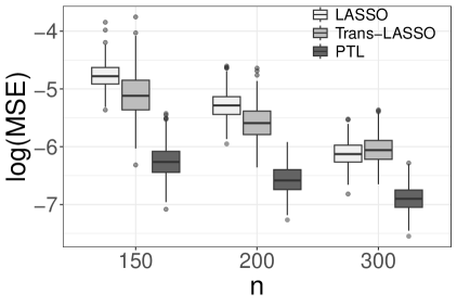
(a) $N=1500$ and $s=40$

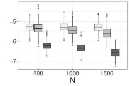
(b) $n=200$ and $s=40$

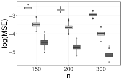
(c) $N=1500$ and $s=300$

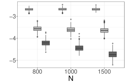
(d) $n=200$ and $s=300$

Figure 1: The boxplots of the log-transformed MSE values for three different estimators $\widehat{\beta}_{\text{lasso}}$, $\widehat{\beta}_{\text{tlasso}}$ and $\widehat{\beta}_{\text{ptl}}$ in Example 1. The first row presents the sparse cases with $s=40$ and the second row presents the dense cases when $s=300$. The first and second columns study the target sample size $n$ and the source sample size $N$, respectively.

Example 1. This is an example revised from Li et al. (2022) and Tripuraneni et al. (2021). Specifically, we generate $\bm{\beta}$ by the following two steps.

• Generate $B$. Let $\Omega=(\omega_{ij})_{r_{0}\times K}$ be an $r_{0}\times K$ matrix with $\omega_{ij}$ independently generated from standard normal distribution. Let $U_{K}=(u_{1},\dots,u_{K})\in\mathbb{R}^{r_{0}\times K}$ be the first $K$ left singular vector of $\Omega$ with $\|u_{k}\|=1$ for $1\leq k\leq K$. Then set $B=(2U_{K}^{\top},0.3\bm{1}_{s-r_{0},K}^{\top},\bm{0}_{p-s,K}^{\top})^{\top}\in\mathbb{R}^{p\times K}$ (Tripuraneni et al., 2021).

• Generate $\bm{\delta}$ and $\bm{\beta}$. Specifically, $\bm{\delta}=(\delta_{1},\dots,\delta_{p})^{\top}$ is generated as follows. Let $\mathcal{S}$ be an index set with $|\mathcal{S}|=s_{\delta}$ randomly sampled from $\{s+1,\dots,p\}$ without replacement. Next, for each $j\in\mathcal{S}$, we generate $\delta_{j}$ independently from $N(0,h/s_{\delta})$. For each $j\notin\mathcal{S}$, set $\delta_{j}=0$ (Li et al., 2022). The target parameter is then assembled by $\bm{\beta}=B\bm{w}+\bm{\delta}$ with $\bm{w}=(3/2,3/4,0,0,-5/4)^{\top}\in\mathbb{R}^{5}$. When $s_{\delta}$ is small, the difference between $\mbox{supp}(\bm{\beta})$ and $\mbox{supp}(\bm{\beta}^{(k)})$ is only $s_{\delta}$ elements.

Set $\Sigma_{k}=\Sigma=I_{p}$ (Tripuraneni et al., 2021) and $\sigma_{k}^{2}=\sigma^{2}=1$ for $1\leq k\leq K$. Fix the source sample size $n_{k}\equiv N$ to be the same for $1\leq k\leq K$. Consider different $n\in\{150,200,300\}$ and $N\in\{800,1000,1500\}$. Set $r_{0}=\lfloor s/3\rfloor$ and $s_{\delta}=\lfloor s/5\rfloor$ with $s=40$ (sparse) and $s=300$ (dense), respectively. Here $\lfloor x\rfloor$ stands for the largest integer no greater than $x$. The experiment is then randomly replicated for a total of $B=500$ times. This leads to a total of 500 MSE values, which are then log-transformed and boxplotted in Figure 1.

By Figure 1, we find that the MSE values of both the Trans-LASSO and the PTL estimators are consistently smaller than those of the LASSO estimator. This is reasonable because LASSO uses only the target data, while Trans-LASSO and PTL utilize the information from both the target and the sources. Secondly, MSE values of Trans-LASSO and PTL decrease as $N$ increases; see the right top and right bottom panels. This suggests that a larger source sample size also helps to improve the estimation accuracy of the target parameter significantly for the Trans-LASSO and PTL method. Lastly and also most importantly, for all the simulation cases, the MSE values of the PTL estimator are clearly smaller than those of the other estimators. This suggests that the PTL estimator is the best choice compared with two other competitors for this particular case.

Example 2. For this example, we allow the supports of the source and target parameters to be very different. Specifically, we generate $\bm{\beta}^{(k)}$’s and $\bm{\beta}$ by the following two steps.

• Generate $B$. Specifically, we generate an $s\times K$ random matrix $\Omega$ in the same way as in Example 1. Denote its first $K$ left singular vectors by $U_{K}=(u_{1},\dots,u_{K})\in\mathbb{R}^{s\times K}$ with $u_{k}=(u_{k1},\dots,u_{ks})^{\top}\in\mathbb{R}^{s}$ and $\|u_{k}\|=1$. The support of $\bm{\beta}^{(k)}$ is given by $\mathcal{S}_{c}\cup\mathcal{S}_{k}$, where $\mathcal{S}_{c}$ denotes the common support set shared by all sources and $\mathcal{S}_{k}$ stands for the support set uniquely owned by source $k$. Define $s_{c}=|\mathcal{S}_{c}|$ the cardinality of $\mathcal{S}_{c}$. Let $\mathcal{S}_{k}=\{s_{k,1},\dots,s_{k,s-s_{c}}\}$ be a random subset of $\{s_{c}+1,\dots,p\}$ without replacement. Set $\beta_{j}^{(k)}=2u_{kj}$ for $1\leq j\leq s_{c}$, $\beta_{s_{k,j}}^{(k)}=2u_{k,j+s_{c}}$ for $1\leq j\leq s-s_{c}$ and $\beta^{(k)}_{j}=0$ if $j\notin\mathcal{S}_{c}\cup\mathcal{S}_{k}$. Set $B=(\bm{\beta}^{(1)},\dots,\bm{\beta}^{(K)})\in\mathbb{R}^{p\times K}$.

• Generate $\bm{\delta}$ and $\bm{\beta}$. Let $\mathcal{S}_{0}$ be a random subset of $\{1,\dots,p\}$ without replacement with $|\mathcal{S}_{0}|=s_{\delta}$. Let $\widetilde{\delta}\in\mathbb{R}^{s_{\delta}}$ be the last eigenvector of $B_{\mathcal{S}_{0}}B_{\mathcal{S}_{0}}^{\top}$, where $B_{\mathcal{S}_{0}}=(\beta^{(1)}_{\mathcal{S}_{0}},\dots,\beta^{(K)}_{\mathcal{S}_{0}})$ and $\beta^{(k)}_{\mathcal{S}_{0}}=(\beta_{j}:j\in\mathcal{S}_{0})^{\top}\in\mathbb{R}^{s_{\delta}}$. Fix $\bm{\delta}$ to be $\delta_{\mathcal{S}_{0}}=h\widetilde{\delta}/|\widetilde{\delta}|$ and $\delta_{\mathcal{S}_{0}^{c}}=0$. Therefore, the identification condition about delta (i.e. $B^{\top}\Sigma\bm{\delta}=0$) can be naturally satisfied. The target parameter is then assembled as $\bm{\beta}=B\bm{w}+\bm{\delta}$ with $w=(3/2,3/4,0,0,-5/4)^{\top}\in\mathbb{R}^{5}$.

The specification of $\Sigma,\Sigma_{k},\sigma^{2}$ and $\sigma_{k}^{2}$ are the same as in Example 1. The experiment is then randomly replicated for a total of $B=500$ times. This leads to a total of 500 MSE values, which are then log-transformed and boxplotted in Figure 2.

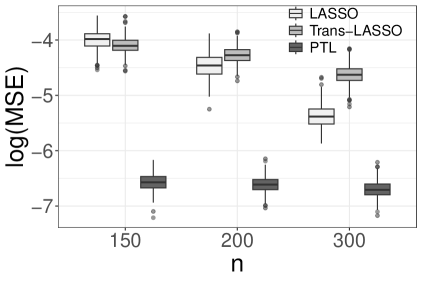
(a) $n_{s}=800$ and $s=40$

(b) $n=200$ and $s=40$

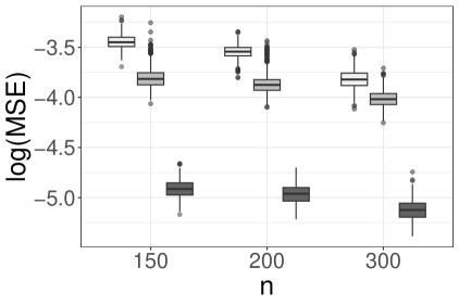
(c) $n_{s}=800$ and $s=300$

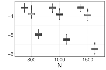
(d) $n=200$ and $s=300$

Figure 2: The boxplots of the log-transformed MSE values for four different estimators $\widehat{\beta}_{\text{lasso}}$, $\widehat{\beta}_{\text{tlasso}}$ and $\widehat{\beta}_{\text{ptl}}$ in Example 2. The first row presents the sparse cases with $s=40$ and the second row presents the dense cases when $s=300$. The first and second columns study the target sample size $n$ and the source sample size $N$, respectively.

Most numerical findings obtained by Figure 2 are qualitatively similar to those of Figure 1. The key differences are given by the right two panels, where as the source data sample size $N$ increases, the decreases of $\log(\mbox{MSE})$ for the Trans-LASSO estimator is small. This suggests that the transfer learning capability of the Trans-LASSO estimator is very limited for this particular example. The success of the Trans-LASSO method heavily hinges on the vanishing-difference assumption, which is unfortunately violated seriously in this example. Similar patterns are also observed for the LASSO estimator. In contrast, the $\log(\mbox{MSE})$ values for PTL estimator steadily decrease as $n_{s}$ increases. The PTL method once again stands out clearly as the best method for this particular case.

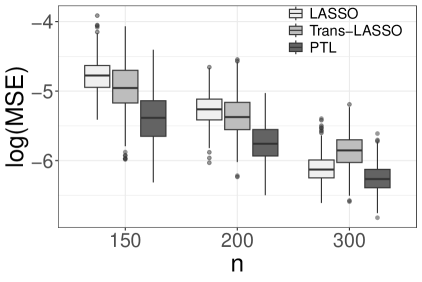
(a) $N=1500$ and $s=30$

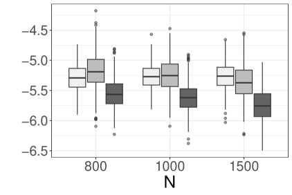
(b) $n=200$ and $s=30$

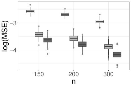
(c) $N=1500$ and $s=300$

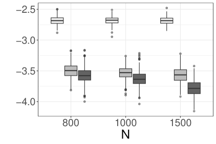
(d) $n=200$ and $s=300$

Figure 3: The boxplots of the log-transformed MSE values for four different estimators $\widehat{\beta}_{\text{lasso}}$, $\widehat{\beta}_{\text{tlasso}}$ and $\widehat{\beta}_{\text{ptl}}$ in Example 3. The first row presents the sparse cases with $s=40$ and the second row presents the dense cases when $s=300$. The first and second columns study the target sample size $n$ and the source sample size $N$, respectively.

Example 3. For this example, the parameter specifications here are the same as those of Example 1. The key difference is that the covariance matrices of covariates are allowed to be different for the target and source datasets. Moreover, the error variances are also allowed to be different for different datasets. Specifically, we generate $\Sigma_{k}$, $\Sigma$, $\sigma_{k}^{2}$ and $\sigma^{2}$ as follows.

• Generate $\Sigma_{k}$ and $\Sigma$. For source $k$, set $\Sigma_{k}$ to be a symmetric Toeplitz matrix with first row given by $(1,\bm{1}_{2k-1}^{\top}/(k+1),\bm{0}_{p-2k}^{\top})$, where $\bm{1}_{2k-1}=(1,\dots,1)^{\top}\in\mathbb{R}^{2k-1}$ for $1\leq k\leq K$; see Section 8.3.4 of Seber (2008) for more details. For the target dataset, set the covariance matrix of the covariates as $\Sigma=I_{p}$ (Li et al., 2022).

• Generate $\sigma_{k}^{2}$ and $\sigma^{2}$. Set the error variance of the $k$th source as $\sigma_{k}^{2}=k$. Fix $\sigma^{2}=1$ for the target data.

The experiment is then randomly replicated for a total of $B=500$ times. This leads to a total of 500 MSE values, which are then log-transformed and boxplotted in Figure 3. The numerical findings obtained in Figure 3 are similar to those of Figure 1. The proposed PTL estimator remains to be the best one.

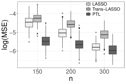
(a) $N=1500$ and $s=30$

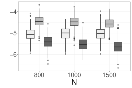
(b) $n=200$ and $s=30$

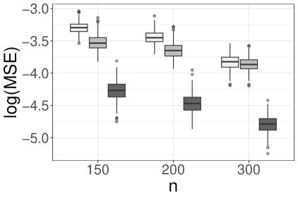
(c) $N=1500$ and $s=300$

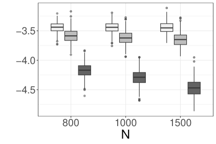
(d) $n=200$ and $s=300$

Figure 4: The boxplots of the log-transformed MSE values for four different estimators $\widehat{\beta}_{\text{lasso}}$, $\widehat{\beta}_{\text{tlasso}}$ and $\widehat{\beta}_{\text{ptl}}$ in Example 4. The first row presents the sparse cases with $s=40$ and the second row presents the dense cases when $s=300$. The first and second columns study the target sample size $n$ and the source sample size $N$, respectively.

Example 4 In this example, we consider the case the parameter generation is different from the identification condition. Specifically, the parameter $\bm{\beta}^{(k)}$’s and $\bm{\beta}$ are generated as follows.

• Generate $B$. The way for generating $B$ is the same as Example 1. Generate $\bm{\delta}$ and $\bm{\beta}$ as follows. The generation of $\bm{\delta}^{*}$ is similar to that of $\bm{\delta}$ in Example 1 expect for $\mathcal{S}$ is sampled from $\{1,\dots,p\}$. Set $\bm{\beta}=B\bm{w}^{*}+\bm{\delta}^{*}$ with $\bm{w}^{*}=(3/2,3/4,0,0,-5/4)^{\top}\in\mathbb{R}^{5}$.

• Generate $\Sigma_{k}$, $\Sigma$, $\sigma_{k}^{2}$ and $\sigma^{2}$. Set $\Sigma_{k}$’s the same as those in Example 3. Set $\Sigma=(\sigma_{ij})_{p\times p}$ with $\sigma_{ij}=0.5^{|i-j|}$. In this scenario, the identification condition $B^{\top}\Sigma\bm{\delta}^{*}=\mathbf{0}$ does not hold. Set $\sigma_{k}^{2}=1.25^{k-3}$ and $\sigma^{2}=1$.

The experiment is then randomly replicated for a total of $B=500$ times. This leads to a total of 500 MSE values, which are then log-transformed and boxplotted in Figure 4. We find that although the identification condition is violated, the proposed PTL estimator remains to be the best estimator.

4.3. Real Data Analysis

We study here the problem of sentence prediction for fraud crimes occurred in China rendered in the year from 2018 to 2019. Fraud is one of the most traditional types of property crime, characterized by a high proportion and a wide variety. For example, from 2018 to 2019, fraud accounted for approximately 1% of all recorded criminal activities. In Chinese criminal law, besides the basic fraud crime, offenses related to fraud crime include contract fraud, insurance fraud, credit card fraud, and many other types. As the societal harm caused by different categories of fraudulent behavior varies, the sentencing guidelines also differ. Consequently, it becomes particularly important to make scientifically reasonable sentencing judgments for a given case of fraud, serving as a crucial guarantee for judicial fairness and justice. However, given the complexity and variety of different fraud cases, judges need to make their final judicial rulings based on the facts of the crime, relevant legal statutes, and their necessary personal judgment. The involvement of personal subjective judgment often leads to considerable uncertainty in judicial decisions, indirectly impacting the fairness and justice of judicial practices. Therefore, it is crucial to construct an objective, precise, and automated sentencing model to assist judges in making more scientifically stable and fair sentencing decisions.

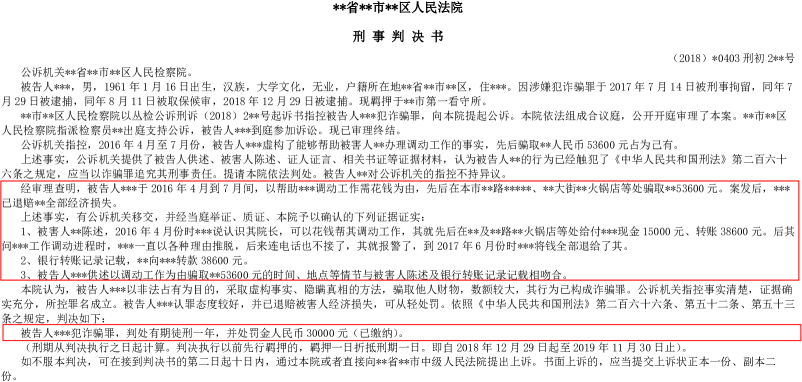
Figure 5: An illustration for judgment document. The middle box highlights the major facts. The bottom box highlights the sentencing decisions.

To this end, we consider training different linear regression models for different types of fraud. Specifically, our data are collected from China Judgment Online (CJO, https://wenshu.court.gov.cn/) during the period from 2018 to 2019. For simplicity, only the first trials and fixed-term imprisonment cases are considered. Here, we use the log-transformed length of sentence as the dependent variable, which is extracted from the document; see the bottom box in Figure 5 for illustration. Subsequently, we convert the text in the sentencing documents related to the criminal facts (see middle box in Figure 5) into high-dimensional 1536-dimensional vectors using the OpenAI text-embedding-ada-02 model (https://openai.com/blog/new-and-improved-embedding-model). After that, different high-dimensional linear regression models can be established for various types of fraud. It is worth noting that the proportions of different types of fraud in the entire sample are very different from each other. A few of the most common types of fraud occupy a large proportion of the whole sample. For instance, the crime of fraud accounts for 71.8% of the total fraud cases and crime of contract fraud accounts for 9.7%; see Table 1 for details. Therefore, the sample sizes for these few types of frauds are relatively sufficient for accurate estimation. Unfortunately, there are a large number of other types of frauds with tiny sample sizes. Consider for example the crime of negotiable instrument fraud, the corresponding sample size is only 112. This tiny sample size is obviously insufficient to support precise parameter estimation.

[b] Crime Type  Sample Size $n$  Percentage (%) Crime of Fraud 37,121 71.80 Crime of Contract Fraud 5,014 9.70   Crime of Making out False Invoices¹ 3,827 7.40 Crime of Credit Card Fraud 3,816 7.38 Crime of Cheating and Bluffing 586 1.13 Crime of Fund-Raising Fraud 537 1.04 Crime of Insurance Fraud 373 0.72 Crime of Loan Fraud 192 0.37 Crime of Defrauding Loans² 126 0.24 Crime of Negotiable Instrument Fraud 112 0.22

Table 1: Different Types of Fraud Crimes

• The full name is Crime of Making out False Value-Added Tax Invoices or Other False Invoices to Obtain an Export Tax Refund or to Offset Payable Taxes.

• The full name is Crime of Defrauding Loans, Acceptance of Negotiable Instruments and Financial Document or Instrument.

To overcome this challenge, we consider here the method of transfer learning. Specifically, we treat fraud categories with sample sizes exceeding 1000 as the source datasets, while the other small categories as target datasets. This leads to a total of 4 source datasets, corresponding to the crime of fraud, crime of contract fraud, crime of making out false invoices, and crime of credit card fraud. The corresponding sample sizes are given by 37,121, 5,014, 3,827 and 3,816, respectively. Then, we attempt to employ the PTL estimator proposed in this paper to borrow the information from the source datasets to help the target models. To evaluate the prediction performance of the proposed PTL method, we apply the two-fold cross validation method. For the training dataset, we estimate the regression coefficients by the PTL method. For the validation dataset, we evaluate the prediction performance by out-of-sample $R$-squared, defined as $R^{2}_{\text{val}}=1-\sum_{i\in\mathcal{S}_{\text{val}}}(\widehat{Y}_{i}-Y_{i})^{2}/\sum_{i\in\mathcal{S}_{\text{val}}}(Y_{i}-\bar{Y}_{\text{val}})^{2}$. Here $\mathcal{S}_{\text{val}}$ is the index of validation dataset and $\bar{Y}_{\text{val}}$ is the sample mean of the validation response. This procedure is replicated for a total of 100 times, resulting in a total of 200 out-of-sample $R$-squared values. For comparison purpose, the LASSO and Trans-LASSO estimators are also tested. The average $R$-squared values are reported in Table 2. By Table 2, we find that the PTL estimators outperform the other two estimators for all target crimes.

[b] Crime Type $n$ LASSO Trans-LASSO PTL Crime of Cheating and Bluffing 586 12.41 16.85 25.90 Crime of Fund-Raising Fraud 537 2.16 4.83 12.90 Crime of Insurance Fraud 373 3.78 12.05 14.64 Crime of Loan Fraud 192 -0.34 10.95 18.60 Crime of Defrauding Loans¹ 126 -5.19 0.56 1.78 Crime of Negotiable Instrument Fraud 112 3.94 27.92 30.08

Table 2: Average out-sample $R$-squared (%) for different methods.

• The full name of the crime is Crime of Defrauding Loans, Acceptance of Negotiable Instruments and Financial Document or Instrument.

5. CONCLUDING REMARKS

In this article, we present here a profiled transfer learning method. The non-asymptotic upper bound and minimax lower bound are established. The proposed estimator is minimax optimal under appropriate conditions. Numerical studies and a real data example about sentence prediction are presented to demonstrate the finite sample performance of the proposed method. To conclude this article, we consider several interesting topics for future research. First, we use all the source datasets to construct the profiled response. However, the source datasets could be useless if its regression pattern is extremely different from the target one. Therefore, there is a practical need to select the useful source datasets by appropriate method. This seems the first interesting topic for future study. Second, we studied here linear regression model only. Then how to generalize the method of profiled transfer learning to other statistical models (e.g. a logistic regression model) is another interesting topic for future study. Lastly, high dimensional covariance estimation is another important statistical problem suffering from the curse of dimensionality. Then how to conduct profiled transfer learning for high dimensional covariance estimator is also an important topic worthwhile pursuing.

Supplementary Materials to “Profiled Transfer Learning for High Dimensional Linear Model”

Recall that $\bm{\beta}=B\bm{w}+\bm{\delta}$, we can rewrite the model as $Y_{i}=X_{i}^{\top}B\bm{w}+X_{i}^{\top}\bm{\delta}+\varepsilon_{i}$. Multiply $B^{\top}X_{i}$ on both sides and take expectation, we have $B^{\top}E(X_{i}Y_{i})=B^{\top}\Sigma B\bm{w}$. Note that $B^{\top}\Sigma B$ is nonsingular since the $\bm{\beta}^{(k)}$’s are linearly independent and $\Sigma$ is positive definite. As a result, the vector $\bm{w}$ be can identified as $\bm{w}=(B^{\top}\Sigma B)^{-1}B^{\top}E(X_{i}Y_{i})$.

Next we consider the identification of $\bm{\delta}$. Multiply $X_{i}$ on both sides of $Y_{i}=X_{i}^{\top}B\bm{w}+X_{i}^{\top}\bm{\delta}+\varepsilon_{i}$ and take expectation, we have $E(X_{i}Y_{i})=\Sigma B\bm{w}+\Sigma\bm{\delta}$. Then the vector $\bm{\delta}$ can be identified as $\bm{\delta}=\Sigma^{-1}\{E(X_{i}Y_{i})-\Sigma B\bm{w}\}$. The proof is completed.

To prove the theorem condition, we first introduce several useful lemmas.

Lemma 1.

(Generalized Hanson-Wright Inequality) Assume that $X\in\mathbb{R}^{p}$ is a mean zero sub-Gaussian random vector with $\|X\|_{\psi_{2}}\leq C_{\psi_{2}}$. Let $B\in\mathbb{R}^{p\times K}$ be an arbitrary constant matrix, then we have $E\exp(\lambda^{2}\|B^{\top}X\|^{2})\leq\exp(C_{1}C_{\psi_{2}}^{2}\lambda^{2}\|B\|^{2}_{F})$ for all $|\lambda|\leq C_{2}/(C_{\psi_{2}}\|B\|_{\text{op}})$, where $C_{1}>0$ and $C_{2}>0$ are some fixed positive constants.

Proof.

This lemma comes from Exercise 6.2.6 in Vershynin (2018). For the sake of completeness, we provide here a brief proof for the lemma. The proof is based on the results of Hsu et al. (2012). Define $A=(B,\mathbf{0}_{p\times(p-K)})\in\mathbb{R}^{p\times p}$. Then $\|A^{\top}X\|^{2}=X^{\top}AA^{\top}X=X^{\top}BB^{\top}X=\|B^{\top}X\|^{2}$, $\|A\|_{\text{op}}=\|B\|_{\text{op}}$ and $\|A\|_{F}=\|B\|_{F}$. As a result, the inequalities in Hsu et al. (2012) holds for matrix $B\in\mathbb{R}^{p\times K}$. Then by condition (C2), we know that $E\exp(u^{\top}X_{i})\leq\exp(C_{3}C_{\psi_{2}}^{2}\|u\|^{2}/2)$ for some constant $C_{3}>0$. Next by Remark (2.3) of Hsu et al. (2012), for $|\lambda|<1/(\sqrt{2C_{3}}C_{\psi_{2}}\|B\|_{\text{op}})$, we have

$$E\exp(\lambda^{2}\|B^{\top}X\|^{2})\leq\exp\bigg{\{}C_{3}C_{\psi_{2}}^{2}\|B\|_{F}^{2}\lambda^{2}+\frac{C_{3}^{2}C_{\psi_{2}}^{4}\lambda^{4}\|B\|_{\text{op}}^{2}\|B\|_{F}^{2}}{1-2C_{3}C_{\psi_{2}}^{2}\|B\|_{\text{op}}^{2}\lambda^{2}}\bigg{\}}.$$

When $|\lambda|\leq 1/(\sqrt{3C_{3}}C_{\psi_{2}}\|B\|_{\text{op}})$, we then have $C_{3}^{2}C_{\psi_{2}}^{4}\|B\|_{\text{op}}^{2}\lambda^{4}/(1-2C_{3}C_{\psi_{2}}^{2}\|B\|_{\text{op}}^{2}\lambda^{2})\leq C_{3}C_{\psi_{2}}^{2}\lambda^{2}$. As a result, we have $E\exp(\lambda^{2}\|BX\|^{2})\leq\exp(2C_{3}C_{\psi_{2}}^{2}\lambda^{2}\|B\|_{F}^{2})$. Take $C_{1}=2C_{3}$ and $C_{2}=1/\sqrt{3C_{3}}$, then the lemma proof is complete.
∎

Lemma 2.

(Convergence Rate of Sample Covariance Matrix) Let $Z_{1},Z_{2},\dots\in\mathbb{R}^{K}$ be a sequence of independent and identically distributed zero-mean sub-Gaussian random vectors. Suppose there exists some fixed constant $M\geq 1$ such that $\|u^{\top}Z_{i}\|_{\psi_{2}}\leq ME(u^{\top}Z_{i})^{2}$ for all $u\in\mathbb{R}^{p}$. Define $\widehat{\Sigma}_{Z}=n^{-1}\sum_{i=1}^{n}Z_{i}Z_{i}^{\top}$ and $\Sigma_{Z}=E(Z_{i}Z_{i}^{\top})$. Then for every positive integer $n$, we have

$$\|\widehat{\Sigma}_{Z}-\Sigma_{Z}\|_{\text{op}}\leq CM^{2}\Bigg{(}\sqrt{\frac{K+t}{n}}+\frac{K+t}{n}\Bigg{)}\|\Sigma_{Z}\|_{\text{op}}$$

with probability at least $1-2\exp(-t)$ for some constant $C>0$.

Proof.

This result comes from Exercise 4.7.3 of Vershynin (2018). For the sake of completeness, we provide a here a brief proof. Let $U_{i}=\Sigma_{Z}^{-1/2}Z_{i}$. Then by lemma condition, we have $E(U_{i})=0$, $\mbox{cov}(U_{i})=I_{K}$ and $\|U_{i}\|_{\psi_{2}}\leq M$. Define $\widehat{\Sigma}_{u}=n^{-1}\sum_{i=1}^{n}U_{i}U_{i}^{\top}$ Then by Theorem 4.6.1 of Vershynin (2018), we have $\|\widehat{\Sigma}_{u}-I_{K}\|_{\text{op}}\leq M^{2}\max\{\delta,\delta^{2}\}$ with probability $1-2\exp(-u)$, where $\delta=C_{0}(\sqrt{K/n}+\sqrt{u/n})$ for some constant $C_{0}>0$. Let $C=\max\{\sqrt{2}C_{0},2C_{0}^{2}\}$, we have $\|\widehat{\Sigma}_{u}-I_{K}\|_{\text{op}}\leq CM^{2}\{\sqrt{K+u/n}+(K+u)/n\}$ with probability $1-2\exp(-u)$. Then $\|\widehat{\Sigma}_{Z}-\Sigma_{Z}\|_{\text{op}}\leq\|\widehat{\Sigma}_{u}-I_{K}\|_{\text{op}}\|\Sigma_{Z}\|_{\text{op}}\leq CM^{2}\{\sqrt{K+u/n}+(K+u)/n\}\|\Sigma_{Z}\|_{\text{op}}$ with probability $1-2\exp(-u)$.
∎

Lemma 3.

(Restricted Strong Convexity for Correlated Sub-Gaussian Features) Let $X_{1},X_{2},\dots,X_{n}\in\mathbb{R}^{p}$ be a sequence of independent and identically distributed zero-mean sub-Gaussian random vectors with $E(X_{i}X_{i}^{\top})=\Sigma$ and $\|X_{i}\|_{\psi_{2}}\leq C_{\psi_{2}}$. Define $\widehat{\Sigma}=n^{-1}\sum_{i=1}^{n}X_{i}X_{i}^{\top}$. If $n\geq C_{1}\max\{C_{\psi_{2}}^{4}/\lambda_{\min}(\Sigma),1\}\log p$ for some constant $C_{1}>0$. Then for any $u\in\mathbb{R}^{p}$ there exists a universal constant $C>0$ such that

$$u^{\top}\widehat{\Sigma}u\geq\frac{\lambda_{\min}(\Sigma)}{2}\|u\|^{2}-C\lambda_{\min}^{2}(\Sigma)\max\bigg{\{}\frac{C_{\psi_{2}}^{4}}{\lambda_{\min}^{2}(\Sigma)},1\bigg{\}}\bigg{(}\frac{\log p}{n}\bigg{)}\|u\|_{1}^{2}$$

with probability at least $1-2\exp(-\log p)$.

Proof.

The proof of the lemma could be derived by Lemma 1 of Loh and Wainwright (2012) and be found in Lemma B.2 of Zhu (2018). ∎

Lemma 4.

(Convergence Rate of $\widehat{\bm{w}}_{\text{ptl}}$) Under the same conditions as in Theorem 1, then there exist constants $C_{0}$, $C_{1},C_{2}$ and $C_{3}$ such that for any $t\leq C_{0}n$, we have $P(\|\widehat{\bm{w}}_{\text{ptl}}-\bm{w}\|^{2}\leq C_{1}\sum_{k=1}^{K}s_{\max}\log p/n_{k}+C_{2}(K+t)/n)\geq 1-\exp(-C_{3}t)$.

Proof.

Recall that $\widehat{\bm{w}}_{\text{ptl}}=\mbox{argmin}_{\bm{w}}\mathcal{L}_{w}(\bm{w},\widehat{Z})$. Then by standard ordinary least squares, we have

$$\widehat{\bm{w}}_{\text{ptl}} = \Big{(}n^{-1}\sum_{i=1}^{n}\widehat{Z}_{i}\widehat{Z}_{i}^{\top}\Big{)}^{-1}\Big{\{}n^{-1}\sum_{i=1}^{n}\widehat{Z}_{i}(Y_{i}-\widehat{Z}_{i}^{\top}w)\Big{\}}$$

$$= \bm{w}+\widehat{\Sigma}_{\widehat{Z}}^{-1}(Q_{1}+Q_{2}+Q_{3}),$$

where $\widehat{\Sigma}_{\widehat{Z}}=n^{-1}\sum_{i=1}^{n}\widehat{Z}_{i}\widehat{Z}_{i}^{\top}$, $Q_{1}=n^{-1}\sum_{i=1}^{n}\widehat{Z}_{i}(Z_{i}-\widehat{Z}_{i})^{\top}\bm{w}$, $Q_{2}=n^{-1}\sum_{i=1}^{n}\widehat{Z}_{i}X_{i}^{\top}\bm{\delta}$ and $Q_{3}=n^{-1}\sum_{i=1}^{n}\widehat{Z}_{i}\varepsilon_{i}$. We next evaluated the quantities $\widehat{\Sigma}_{\widehat{Z}}$, $Q_{1}$, $Q_{2}$ and $Q_{3}$ subsequently. The desired conclusion follows if we can show the following conclusions hold with probability at least $1-\exp(-C_{3}t)$: (1) $\lambda_{\min}(\widehat{\Sigma}_{\widehat{Z}})\geq\tau_{\min}$; (2) $\|Q_{1}\|\leq\tau_{\max}(\sum_{k=1}^{K}s_{\max}\log p/n_{k})^{1/2}$; (3) $\|Q_{2}\|\leq\tau_{\max}h[(\sum_{k=1}^{K}s_{\max}\log p/n_{k})^{1/2}+\{(K+t)/n\}^{1/2}]$; and (4) $\|Q_{3}\|\leq\tau_{\max}\{(K+t)/n\}^{1/2}$ for some positive constants $\tau_{\max},\tau_{\min}>0$.

Step 1. We first consider the term $\widehat{\Sigma}_{\widehat{Z}}=\Sigma_{Z}+\Delta_{z1}+\Delta_{z2}+\Delta_{z2}^{\top}+\Delta_{z3}$, where $\Sigma_{Z}=E(Z_{i}Z_{i}^{\top})=B^{\top}\Sigma B$, $\Delta_{z1}=n^{-1}\sum_{i=1}^{n}(\widehat{Z}_{i}-Z_{i})(\widehat{Z}_{i}-Z_{i})^{\top}$, $\Delta_{z2}=n^{-1}\sum_{i=1}^{n}Z_{i}(\widehat{Z}_{i}-Z_{i})^{\top}$ and $\Delta_{z3}=n^{-1}\sum_{i=1}^{n}Z_{i}Z_{i}^{\top}-\Sigma_{Z}$. Then we next show that $\|\Delta_{zj}\|_{\text{op}}=o(1)$ for $j=1,2,3$ with high probability as follows.

Step 1.1. We begin with $\Delta_{z1}$. By triangle inequality, we have $\|\Delta_{z1}\|_{F}^{2}\leq n^{-1}\sum_{i=1}^{n}\|\widehat{Z}_{i}-Z_{i}\|^{2}=n^{-1}\sum_{i=1}^{n}\|(\widehat{B}-B)^{\top}X_{i}\|^{2}$. Note that $\widehat{B}-B$ is independent with $X_{i}$. Then by Lemma 1, we know that conditional on $\widehat{B}-B$, $\|(\widehat{B}-B)X_{i}\|^{2}$ is sub-exponential with $\Big{\|}\|(\widehat{B}-B)^{\top}X_{i}\|^{2}\Big{\|}_{\psi_{1}}\leq C_{1}\|\widehat{B}-B\|_{F}^{2}\|X_{i}\|_{\psi_{2}}^{2}\leq C_{1}C_{\psi_{2}}^{2}\|\widehat{B}-B\|_{F}^{2}$ for some constant $C_{1}>0$, where $\|U\|_{\psi_{1}}=\inf\{t>0:E\exp(|U|/t)\leq 2\}$ is the sub-exponential norm of a sub-exponential random variable. Then by Bernstein’s inequality (Vershynin, 2018) and condition (C2), we have

$$P\bigg{(}n^{-1}\sum_{i=1}^{n}\Big{\|}(\widehat{B}-B)X_{i}\Big{\|}^{2}-\mbox{tr}\Big{\{}(\widehat{B}-B)\Sigma(\widehat{B}-B)^{\top}\Big{\}}\geq C_{1}C_{\psi_{2}}^{2}\|\widehat{B}-B\|_{F}^{2}\bigg{)}\leq\exp(-c_{1}n)$$

for some constant $c_{1}>0$. Note that if $A\leq B$, then $\mbox{tr}(A)\leq\mbox{tr}(B)$ for two arbitrary symmetric matrices $A,B\in\mathbb{R}^{p\times p}$ (Seber, 2008). Then by condition (C4), we have $\mbox{tr}\{(\widehat{B}-B)\Sigma(\widehat{B}-B)^{\top}\}\leq C_{\max}\|\widehat{B}-B\|_{F}^{2}$. We have $P(n^{-1}\sum_{i=1}^{n}\|(\widehat{B}-B)X_{i}\|^{2}\geq C_{2}\|\widehat{B}-B\|_{F}^{2})\leq\exp(-c_{1}n)$, where $C_{2}=C_{\max}+C_{1}C_{\psi_{2}}^{2}$. By condition (C4), we can show that $P(\|\widehat{B}-B\|_{F}^{2}\geq C_{3}\sum_{k=1}^{K}s_{\max}\log p/n_{k})\leq\sum_{k=1}^{K}P(\|\widehat{\bm{\beta}}^{(k)}-\bm{\beta}^{(k)}\|^{2}\geq C_{3}s_{\max}\log p/n_{k})\leq\exp(-c_{1}\log p)$ for some $C_{3}>0$. Then we know that

$$P\bigg{(}n^{-1}\sum_{i=1}^{n}\Big{\|}(\widehat{B}-B)X_{i}\Big{\|}^{2}\geq C_{4}\sum_{k=1}^{K}\frac{s_{\max}\log p}{n_{k}}\bigg{)}$$

$$= E\bigg{\{}P\Big{(}n^{-1}\sum_{i=1}^{n}\Big{\|}(\widehat{B}-B)X_{i}\Big{\|}^{2}\geq C_{4}\sum_{k=1}^{K}\frac{s_{\max}\log p}{n_{k}}\Big{|}\widehat{B}-B\Big{)}\bigg{\}}$$

$$\leq P\bigg{(}\|\widehat{B}-B\|_{F}^{2}\geq C_{3}\sum_{k=1}^{K}\frac{s_{\max}\log p}{n_{k}}\bigg{)}$$

$$+ E\bigg{\{}P\Big{(}n^{-1}\sum_{i=1}^{n}\Big{\|}(\widehat{B}-B)X_{i}\Big{\|}^{2}\geq C_{2}\|\widehat{B}-B\|_{F}^{2}\Big{|}\widehat{B}-B\Big{)}\bigg{\}}$$

$$\leq 2\exp(-c_{1}\log p),$$

where $C_{4}=C_{2}C_{3}$ and the last inequality holds by $n\geq\log p$. As a result, we have $P(\|\Delta_{z1}\|_{F}\geq C_{4}\sum_{k=1}^{K}s_{\max}\log p/n_{k})\leq 2\exp(-c_{1}\log p)$.

Step 1.2. Then we consider $\Delta_{z3}$. To apply Lemma 2, we need to bound $\|Z_{i}\|_{\psi_{2}}$, $M$ and $\|\Sigma_{Z}\|_{\text{op}}$. Note that $\|Z_{i}\|_{\psi_{2}}=\sup_{\|u\|=1}\|u^{\top}Z_{i}\|_{\psi_{2}}=\sup_{\|u\|=1}\|u^{\top}B^{\top}X_{i}\|_{\psi_{2}}\leq\sup_{\|u\|=1}\|Bu\|\|X_{i}\|_{\psi_{2}}=\|B\|\|X_{i}\|_{\psi_{2}}\leq C_{\psi_{2}}C_{\max}^{1/2}$. As a result, $Z_{i}$ is sub-Gaussian with $\|Z_{i}\|_{\psi_{2}}\leq C_{\psi_{2}}C_{\max}^{1/2}$. Without loss of generality, we next obtain an upper bound for $M$ when the vector $u\in\mathbb{R}^{p}$ satisfies $\|u\|=1$ (otherwise consider $u_{0}=u/\|u\|$). By condition (C3) and (C4), we have $\|u^{\top}X_{i}\|_{\psi_{2}}^{2}\leq\|X_{i}\|_{\psi_{2}}^{2}\leq C_{\psi_{2}}^{2}\leq C_{\psi_{2}}^{2}C_{\min}^{-1}\lambda_{\min}(\Sigma)\leq C_{\psi_{2}}^{2}C_{\min}^{-1}u^{\top}\Sigma u=C_{\psi_{2}}^{2}C_{\min}^{-1}E(u^{\top}X_{i})^{2}$. Then we know that $\|u^{\top}Z_{i}\|_{\psi_{2}}^{2}=\|(Bu)^{\top}X_{i}\|_{\psi_{2}}^{2}\leq C_{\psi_{2}}^{2}C_{\min}^{-1}E(u^{\top}B^{\top}X_{i})^{2}=C_{\psi_{2}}^{2}C_{\min}^{-1}E(u^{\top}Z_{i})^{2}$. As a result, we know that $M\leq C_{\psi}^{2}C_{\min}^{-1}$. Note that $\|\Sigma_{Z}\|_{\text{op}}=\|B^{\top}\Sigma B\|_{\text{op}}\leq C_{\max}\|B\|_{\text{op}}^{2}\leq C_{\max}^{2}$. Then by Lemma 2, we have

$$P\bigg{(}\|\widehat{\Sigma}_{Z}-\Sigma_{Z}\|_{\text{op}}\geq C_{5}\Big{(}\frac{K+\log p}{n}\Big{)}^{1/2}\bigg{)}\leq\exp(-c_{1}\log p)$$

for some constant $C_{5}>0$. As a result, we know that $P(\|\Delta_{z3}\|_{\text{op}}\geq C_{5}\{(K+\log p)/n\}^{1/2})\leq\exp(-c_{1}\log p)$.

Step 1.3. We next study $\Delta_{z2}$. By Cauchy-Schwarz inequality and note that $\|A\|=\sup_{\|u\|=1,\|v\|=1}u^{\top}Av$ for an arbitrary matrix $A$ (Vershynin, 2018), we can obtain the following inequality

$$\|\Delta_{z2}\|_{\text{op}} = \Big{\|}n^{-1}\sum_{i=1}^{n}Z_{i}(\widehat{Z}_{i}-Z_{i})^{\top}\Big{\|}_{\text{op}}$$

$$= \sup_{\|u\|=1,\|v\|=1}n^{-1}\sum_{i=1}^{n}u^{\top}Z_{i}(\widehat{Z}_{i}-Z_{i})^{\top}v$$

$$\leq \sup_{\|u\|=1,\|v\|=1}\bigg{(}n^{-1}\sum_{i=1}^{n}u^{\top}Z_{i}Z_{i}^{\top}u\bigg{)}^{1/2}\bigg{(}n^{-1}\sum_{i=1}^{n}v^{\top}(\widehat{Z}_{i}-Z_{i})(\widehat{Z}_{i}-Z_{i})^{\top}v\bigg{)}^{1/2}$$

$$\leq \Big{\|}n^{-1}\sum_{i=1}^{n}Z_{i}Z_{i}^{\top}\Big{\|}_{\text{op}}^{1/2}\bigg{(}n^{-1}\sum_{i=1}^{n}\|\widehat{Z}_{i}-Z_{i}\|^{2}\bigg{)}^{1/2}$$

$$\leq \Big{(}\|\widehat{\Sigma}_{Z}-\Sigma_{Z}\|_{\text{op}}+\|\Sigma_{Z}\|_{\text{op}}\Big{)}^{1/2}\bigg{(}n^{-1}\sum_{i=1}^{n}\|\widehat{Z}_{i}-Z_{i}\|^{2}\bigg{)}^{1/2}$$

$$\leq \bigg{\{}C_{5}\Big{(}\frac{K+\log p}{n}\Big{)}^{1/2}+C_{\max}^{2}\bigg{\}}^{1/2}\bigg{(}C_{4}\sum_{k=1}^{K}\frac{s_{\max}\log p}{n_{k}}\bigg{)}^{1/2}$$

with probability $1-3\exp(-c_{1}\log p)$. By condition (C2), we know that $P(\|\Delta_{z3}\|_{\text{op}}\geq C_{6}(\sum_{k=1}^{K}s_{\max}\log p/n_{k})^{1/2})\leq\exp(-c_{1}\log p)$ for some constant $C_{6}>0$.

By condition (C4), we have $\lambda_{\min}(\Sigma_{Z})=\lambda_{\min}(B^{\top}\Sigma B)=\inf_{\|u\|=1}u^{\top}B^{\top}\Sigma Bu\geq C_{\min}\inf_{\|u\|=1}u^{\top}B^{\top}Bu\geq C_{\min}^{2}$. Combining the above results and by condition (C2), we have $\lambda_{\min}(\widehat{\Sigma}_{\widehat{Z}})\geq\lambda_{\min}(\Sigma_{Z})-\|\Delta_{z1}\|_{F}-2\|\Delta_{z2}\|_{\text{op}}-\|\Delta_{z3}\|_{\text{op}}\geq C_{\min}/2$ with probability at least $1-\exp(-c_{2}\log p)$ for some $c_{2}>0$.

Step 2. Then we consider the term $Q_{1}$. We can decompose it into $Q_{1}=Q_{11}+Q_{12}$, where $Q_{11}=n^{-1}\sum_{i=1}^{n}(\widehat{Z}_{i}-Z_{i})(Z_{i}-\widehat{Z}_{i})^{\top}\bm{w}$ and $Q_{12}=n^{-1}\sum_{i=1}^{n}Z_{i}(Z_{i}-\widehat{Z}_{i})^{\top}\bm{w}$. By the proof in Step 1.1, we know that $\|Q_{11}\|=\sup_{\|u\|=1}u^{\top}\Delta_{z1}\bm{w}\leq\|\Delta_{z1}\|_{\text{op}}\|\bm{w}\|\leq\|\Delta_{z1}\|_{F}\|\bm{w}\|\leq C_{4}C_{w}\sum_{k=1}^{K}s_{\max}\log p/n_{k}$ and $\|Q_{12}\|=\sup_{\|u\|=1}u^{\top}\Delta_{z2}\bm{w}\leq\|\Delta_{z2}\|_{\text{op}}\|\bm{w}\|\leq C_{6}C_{w}(\sum_{k=1}^{K}s_{\max}\log p/n_{k})^{1/2}$ with probability at least $1-2\exp(-c_{2}\log p)$.

Step 3. We next consider the term $Q_{2}$. Similarly, it can be decomposed as $Q_{2}=Q_{21}+Q_{22}$, where $Q_{21}=n^{-1}\sum_{i=1}^{n}(\widehat{Z}_{i}-Z_{i})X_{i}^{\top}\bm{\delta}$ and $Q_{22}=n^{-1}\sum_{i=1}^{n}Z_{i}X_{i}^{\top}\bm{\delta}$. Then we consider the two terms subsequently.

Step 3.1. We first consider the term $Q_{21}$. By Cauchy-Schwarz inequality, we have

$$\|Q_{21}\| = \Big{\|}n^{-1}\sum_{i=1}^{n}(\widehat{B}-B)^{\top}X_{i}X_{i}^{\top}\bm{\delta}\Big{\|}$$

$$\leq \Big{\|}n^{-1}\sum_{i=1}^{n}(\widehat{B}-B)^{\top}X_{i}X_{i}^{\top}(\widehat{B}-B)\Big{\|}_{\text{op}}\Big{(}n^{-1}\sum_{i=1}^{n}\bm{\delta}^{\top}X_{i}X_{i}^{\top}\bm{\delta}\Big{)}^{1/2}.$$

By Step 1.1.1, we know that $\|n^{-1}\sum_{i=1}^{n}(\widehat{B}-B)^{\top}X_{i}X_{i}^{\top}(\widehat{B}-B)\|_{\text{op}}\leq n^{-1}\sum_{i=1}^{n}\|X_{i}^{\top}(\widehat{B}-B)\|_{\text{op}}^{2}\leq C_{4}\sum_{k=1}^{K}s_{\max}\log p/n_{k}$ with probability at least $1-2\exp(-c_{1}\log p)$. Note that $\bm{\delta}^{\top}X_{i}$ is sub-Gaussian with $\|\bm{\delta}^{\top}X_{i}\|_{\psi_{2}}\leq\|\bm{\delta}\|\|X_{i}\|_{\psi_{2}}\leq C_{\psi_{2}}\|\bm{\delta}\|_{1}\leq C_{\psi_{2}}h$. As a result, $(\bm{\delta}^{\top}X_{i})^{2}$ is sub-exponential with $\|(\bm{\delta}^{\top}X_{i})^{2}\|_{\psi_{1}}=\|\bm{\delta}^{\top}X_{i}\|_{\psi_{2}}^{2}\leq C_{\psi_{2}}^{2}h^{2}$. Then by Bernstein’s inequality (Vershynin, 2018) and condition (C2), we have

$$P\Big{(}\Big{|}n^{-1}\sum_{i=1}^{n}\bm{\delta}^{\top}X_{i}X_{i}^{\top}\bm{\delta}-\bm{\delta}^{\top}\Sigma\bm{\delta}\Big{|}\geq C_{6}C_{\psi_{2}}^{2}n^{-1}h^{2}\log p\Big{)}\leq 2\exp(-c_{1}\log p)$$

for some constant $C_{6}>0$. Note that $\bm{\delta}^{\top}\Sigma\bm{\delta}\leq C_{\max}\|\bm{\delta}\|^{2}\leq C_{\max}h^{2}$. Then we know that $n^{-1}\sum_{i=1}^{n}\bm{\delta}^{\top}X_{i}X_{i}^{\top}\bm{\delta}\leq h^{2}(C_{\max}+C_{6}C_{\psi_{2}}^{2}n^{-1}\log p)$ with probability at least $1-2\exp(-c_{1}\log p)$. As a result, $\|Q_{21}\|\leq C_{7}h(\sum_{k=1}^{K}s_{\max}\log p/n_{k})^{1/2}$ with probability at least $1-\exp(-c_{1}\log p)$ for some constant $C_{7}\geq C_{4}(C_{\max}+C_{6}C_{\psi_{2}}^{2}n^{-1}\log p)^{1/2}$.

Step 3.2. Then we consider the term $Q_{22}$. We apply the $\varepsilon$-net technique here. For the unit sphere $\mathbb{S}^{K-1}=\{u\in\mathbb{R}^{K}:\|u\|=1\}$. There exists a 1/2-net $\mathcal{N}$ such that $|\mathcal{N}|\leq 5^{K}$. Let $u_{0}\in\mathbb{S}^{K-1}$ satisfying $u_{0}^{\top}Q_{22}=\|Q_{22}\|$. Then there exists a $u\in\mathcal{N}$ such that $\|u-u_{0}\|\leq 1/2$. Then we have $\|Q_{22}\|=|u_{0}^{\top}Q_{22}|\leq|(u_{0}-u)^{\top}Q_{22}|+|u^{\top}Q_{22}|\leq 2^{-1}\|Q_{22}\|+|u^{\top}Q_{22}|$. As a result, we have $\|Q_{22}\|\leq 2\sup_{u\in\mathcal{N}}|u^{\top}Q_{22}|$. Then for a fixed $u\in\mathbb{S}^{n-1}$, consider $u^{\top}Q_{22}=n^{-1}\sum_{i=1}^{n}u^{\top}Z_{i}X_{i}^{\top}\bm{\delta}$. Note that $X_{i}^{\top}\bm{\delta}$ is sub-Gaussian with $\|X_{i}^{\top}\bm{\delta}\|_{\psi_{2}}\leq C_{\psi_{2}}h$. For all $u\in\mathbb{R}^{K}$ satisfying $\|u\|=1$, $u^{\top}Z_{i}$ is sub-Gaussian with $\|u^{\top}Z_{i}\|_{\psi_{2}}\leq\|Z_{i}\|_{\psi_{2}}\leq C_{\psi_{2}}C_{\max}^{1/2}$. As a result $u^{\top}Z_{i}X_{i}^{\top}\bm{\delta}$ is sub-exponential with $\|u^{\top}Z_{i}X_{i}^{\top}\bm{\delta}\|_{\psi_{1}}\leq C_{\psi_{2}}^{2}C_{\max}^{1/2}h$. By Bernstein’s inequality, for all $\eta>0$, we have

$$P\bigg{(}\Big{|}n^{-1}\sum_{i=1}^{n}u^{\top}Z_{i}X_{i}^{\top}\bm{\delta}\bigg{|}\geq\eta hC_{\psi_{2}}C_{\max}^{1/2}\bigg{)}\leq 2\exp\Big{\{}-cn\min(\eta,\eta^{2})\Big{\}}.$$

Then we know that $P(\|Q_{22}\|\geq\eta hC_{\psi_{2}}C_{\max}^{1/2})\leq P(\sup_{u\in\mathcal{N}}|n^{-1}\sum_{i=1}^{n}u^{\top}Z_{i}X_{i}^{\top}\bm{\delta}|\geq\eta hC_{\psi_{2}}C_{\max}^{1/2})\leq 2\times 5^{K}\exp\{-cn\min(\eta,\eta^{2})\}$. Take $\eta=C_{8}\{(K+t)/n\}^{1/2}<1$ for some large enough $C_{8}>0$ such that we have $P(\|Q_{22}\|\geq C_{8}h\{(K+t)/n\}^{1/2})\leq\exp(-c_{1}t)$.

Step 4. Lastly we consider $Q_{3}=Q_{31}+Q_{32}$ where $Q_{31}=n^{-1}\sum_{i=1}^{n}(\widehat{Z}_{i}-Z_{i})\varepsilon_{i}$ and $Q_{32}=n^{-1}\sum_{i=1}^{n}Z_{i}\varepsilon_{i}$. Then we evaluate $Q_{31}$ and $Q_{32}$ subsequently.

Step 4.1. We first consider $Q_{31}$. Similar to the proof in Step 1.2, we know that conditional on $\widehat{B}-B$, $(\widehat{Z}_{i}-Z_{i})=(\widehat{B}-B)^{\top}X_{i}$ is sub-Gaussian with $\|\widehat{Z}_{i}-Z_{i}\|_{\psi_{2}}\leq\|\widehat{B}-B\|\|X_{i}\|_{\psi_{2}}$. Note that $\varepsilon_{i}$ is sub-Gaussian. By a similar proof of Step 3.2, we have

$$P\bigg{(}\|Q_{31}\|\geq C_{9}\Big{(}\frac{K+\log p}{n}\Big{)}^{1/2}\|\widehat{B}-B\|_{\text{op}}\Big{|}\widehat{B}-B\bigg{)}\leq\exp(-c_{1}\log p)$$

for some constant $C_{9}>0$. By Step 1.1, we know that $\|\widehat{B}-B\|_{\text{op}}\leq\|\widehat{B}-B\|_{F}\leq C_{4}\sum_{k=1}^{K}s_{\max}\log p/n_{k}$ with probability $1-2\exp(-c\log p)$. Then by a similar procedure of Step 1.1, we can show that

$$P\Bigg{(}\|Q_{31}\|\geq C_{10}\bigg{(}\frac{K+\log p}{n}\sum_{k=1}^{K}\frac{s_{\max}\log p}{n_{k}}\bigg{)}^{1/2}\Bigg{)}\leq\exp(-c_{1}\log p).$$

Step 4.2. Lastly, we consider $Q_{32}$. Recall that $Z_{i}$ is sub-Gaussian with $\|Z_{i}\|_{\psi_{2}}\leq LC_{\max}^{1/2}$. Then by a similar proof of Step 3.2, we have $P(\|Q_{32}\|\geq C_{11}\{(K+t)/n\}^{1/2})\leq\exp(-c_{1}t)$. Recall that we have shown that $\lambda_{\min}(\widehat{\Sigma}_{\widehat{Z}})\geq C_{\min}/2$ with probability at least $1-\exp(-c_{2}\log p)$. Combining the above results and by the Cauchy-Schwarz inequality, we know that

$$\|\widehat{\bm{w}}_{\text{ptl}}-\bm{w}\|^{2} \leq 2C_{\min}^{-1}(\widehat{\bm{w}}_{\text{ptl}}-\bm{w})^{\top}\widehat{\Sigma}_{\widehat{Z}}(\widehat{\bm{w}}_{\text{ptl}}-\bm{w})$$

$$\leq 2C_{\min}^{-1}\Big{\|}(\widehat{\bm{w}}_{\text{ptl}}-\bm{w})^{\top}\Big{(}Q_{1}+Q_{2}+Q_{3}\Big{)}\Big{\|}$$

$$\leq 2C_{\min}^{-1}\|\widehat{\bm{w}}_{\text{ptl}}-\bm{w}\|\Big{(}\|Q_{1}\|+\|Q_{2}\|+\|Q_{3}\|\Big{)}$$

$$\leq C_{12}\|\widehat{\bm{w}}_{\text{ptl}}-\bm{w}\|\bigg{\{}\Big{(}\sum_{k=1}^{K}\frac{s_{\max}\log p}{n_{k}}\Big{)}^{1/2}+\Big{(}\frac{K+t}{n}\Big{)}^{1/2}\bigg{\}}$$

for some large enough constant $C_{12}>0$ with probability at least $1-\exp\{-(c_{1}+1)\log(n\wedge p)\}$. As a result, we have $P(\|\widehat{\bm{w}}_{\text{ptl}}-\bm{w}\|\leq C_{12}[(\sum_{k=1}^{K}s_{\max}\log p/n_{k})^{1/2}+\{(K+t)/n\}^{1/2}])\geq 1-\exp(-c_{1}t)$.
∎

Lemma 5.

(Convergence Rate of $\widehat{\bm{\delta}}_{\text{ptl}}$) Under the same conditions as in Theorem 1, there exist some positive constants $C_{1}$ and $C_{2}$ such that $P(\|\widehat{\bm{\delta}}_{\text{ptl}}-\bm{\delta}\|^{2}\leq C_{1}(s_{\delta}r_{n}^{2}\wedge hr_{n}\wedge h^{2}))\geq 1-\exp\{-C_{2}\log(n\wedge p)\}$.

Proof.

Define $\widehat{\bm{u}}_{\delta}=\widehat{\bm{\delta}}_{\text{ptl}}-\bm{\delta}$. Note that $\widehat{\bm{\delta}}_{\text{ptl}}=\mbox{argmin}_{\bm{\delta}}\mathcal{L}_{\text{target},\lambda_{\delta}}(\bm{\delta})$. Then we know that $\mathcal{L}_{\text{target},\lambda_{\delta}}(\widehat{\bm{\delta}}_{\text{ptl}})\leq\mathcal{L}_{\text{target},\lambda_{\delta}}(\bm{\delta})$. We then obtain the following relationship

$$\frac{1}{2}\widehat{\bm{u}}_{\delta}^{\top}\widehat{\Sigma}\widehat{\bm{u}}_{\delta} \leq \lambda_{\delta}\|\bm{\delta}\|_{1}-\lambda_{\delta}\|\widehat{\bm{\delta}}_{\text{ptl}}\|_{1}+\Big{|}\widehat{\bm{u}}_{\delta}^{\top}n^{-1}\sum_{i=1}^{n}X_{i}\Big{(}\widehat{e}_{i}-X_{i}^{\top}\bm{\delta}\Big{)}\Big{|}$$

$$\leq \lambda_{\delta}\|\bm{\delta}\|_{1}-\lambda_{\delta}\|\widehat{\bm{\delta}}_{\text{ptl}}\|_{1}+\|\widehat{\bm{u}}_{\delta}\|_{1}\Big{\|}n^{-1}\sum_{i=1}^{n}X_{i}\Big{(}\widehat{e}_{i}-X_{i}^{\top}\bm{\delta}\Big{)}\Big{\|}_{\infty},$$

where $\widehat{\Sigma}=n^{-1}\sum_{i=1}^{n}X_{i}X_{i}^{\top}$. By Lemma 3 and condition (C4), we have

$$\widehat{\bm{u}}_{\delta}^{\top}\widehat{\Sigma}\widehat{\bm{u}}_{\delta} \geq \frac{\lambda_{\min}(\Sigma)}{2}\|\widehat{\bm{u}}_{\delta}\|^{2}-C_{11}\lambda_{\min}(\Sigma)\max\bigg{\{}\frac{C_{\psi_{2}}^{4}}{\lambda_{\min}^{2}(\Sigma)},1\bigg{\}}\frac{\log p}{n}\|\widehat{\bm{u}}_{\delta}\|_{1}^{2}$$ (B.1)

$$\geq \frac{C_{\min}}{2}\|\widehat{\bm{u}}_{\delta}\|^{2}-C_{12}\frac{\log p}{n}\|\widehat{\bm{u}}_{\delta}\|_{1}^{2}$$

with $C_{12}=C_{11}\max\{C_{\psi_{2}}^{4}C_{\min}^{-1},C_{\max}\}$ for some constant $C_{11}>0$ with probability $1-2\exp(-c_{1}\log p)$. Then we are going to show $\|n^{-1}\sum_{i=1}^{n}X_{i}(\widehat{e}_{i}-X_{i}^{\top}\bm{\delta})\|_{\infty}\leq\lambda_{w}$ with high probability. Recall that $\widehat{e}_{i}=Y_{i}-\widehat{Z}_{i}^{\top}\widehat{w}_{\text{ptl}}$ and $Y_{i}=Z_{i}^{\top}\bm{w}+X_{i}^{\top}\bm{\delta}+\varepsilon_{i}$. Then we have

$$\Big{\|}n^{-1}\sum_{i=1}^{n}X_{i}(\widehat{e}_{i}-X_{i}^{\top}\bm{\delta})\Big{\|}_{\infty} = \Big{\|}n^{-1}\sum_{i=1}^{n}X_{i}(Z_{i}^{\top}\bm{w}-\widehat{Z}_{i}^{\top}\widehat{\bm{w}}_{\text{ptl}}+\varepsilon_{i})\Big{\|}_{\infty}$$

$$\leq \Delta_{1}+\Delta_{2}+\Delta_{3}$$

where $\Delta_{1}=\|n^{-1}\sum_{i=1}^{n}X_{i}(Z_{i}-\widehat{Z}_{i})^{\top}\bm{w}\|_{\infty}$, $\Delta_{2}=\|n^{-1}\sum_{i=1}^{n}X_{i}\widehat{Z}_{i}(\bm{w}-\widehat{\bm{w}}_{\text{ptl}})\|_{\infty}$ and $\Delta_{3}=\|n^{-1}\sum_{i=1}^{n}X_{i}\varepsilon_{i}\|_{\infty}$. Then we next show that $P(\Delta_{j}>Cr_{n})\leq\exp(-c_{1}\log p)$ for $j=1,2,3$.

Step 1. We start with $\Delta_{1}$. Note that for $1\leq j\leq p$, conditional on $\widehat{B}-B$, $X_{ij}(Z_{i}-\widehat{Z}_{i})^{\top}\bm{w}$ is sub-exponential with $\|X_{ij}(Z_{i}-\widehat{Z}_{i})^{\top}\bm{w}\|_{\psi_{1}}\leq\|X_{ij}\|_{\psi_{2}}\|(Z_{i}-\widehat{Z}_{i})^{\top}\bm{w}\|_{\psi_{2}}\leq C_{\psi_{2}}^{2}\|\bm{w}\|\|\widehat{B}-B\|_{\text{op}}$. Note that by Cauchy-Schwarz inequality, we have $E\{X_{ij}(Z_{i}-\widehat{Z}_{i})^{\top}w|\widehat{B}-B\}=E\{e_{j}^{\top}X_{i}X_{i}^{\top}(\widehat{B}-B)^{\top}w|\widehat{B}-B\}=e_{j}^{\top}\Sigma(\widehat{B}-B)^{\top}\bm{w}\leq\lambda_{\max}(\Sigma)\|(\widehat{B}-B)^{\top}\bm{w}\|\leq C_{\max}\|\widehat{B}-B\|_{\text{op}}\|\bm{w}\|$, where $e_{j}=(0,\dots,1,\dots,0)^{\top}$ is the canonical basis with the $j$th component equal to 1 otherwise 0. Then by Bernstein’s inequality, we know that

$$P\bigg{(}\bigg{|}n^{-1}\sum_{i=1}^{n}X_{ij}(Z_{i}-\widehat{Z}_{i})^{\top}\bm{w}-E\Big{\{}X_{ij}(Z_{i}-\widehat{Z}_{i})^{\top}\bm{w}\Big{|}\widehat{B}-B\Big{\}}\bigg{|}$$

$$\quad\quad\quad\quad\quad\quad\quad\quad\geq C_{13}C_{\psi_{2}}^{2}\|\bm{w}\|\|\widehat{B}-B\|_{\text{op}}\Big{(}\frac{\log p}{n}\Big{)}^{1/2}\bigg{|}\widehat{B}-B\bigg{)}\leq 2\exp(-c_{1}\log p).$$

As a result, we have

$$P\bigg{(}\Big{|}n^{-1}\sum_{i=1}^{n}X_{ij}(Z_{i}-\widehat{Z}_{i})^{\top}\bm{w}\Big{|}\geq C_{14}\|\bm{w}\|\Big{\|}\widehat{B}-B\Big{\|}_{\text{op}}\bigg{|}\widehat{B}-B\bigg{)}\leq 2\exp\Big{\{}-(c_{1}+1)\log p\Big{\}}$$

for $C_{14}\geq C_{13}C_{\psi_{2}}^{2}(\log p/n)^{1/2}+C_{\max}$. Then by union bound, we know that

$$P\bigg{(}\Delta_{1}\geq C_{14}\|\bm{w}\|\Big{\|}\widehat{B}-B\Big{\|}_{\text{op}}\bigg{|}\widehat{B}-B\bigg{)}$$

$$\leq \sum_{j=1}^{p}P\bigg{(}\Big{|}n^{-1}\sum_{i=1}^{n}X_{ij}\Big{(}Z_{i}-\widehat{Z}_{i}\Big{)}^{\top}\bm{w}\Big{|}\geq C_{14}\|\bm{w}\|\Big{\|}\widehat{B}-B\Big{\|}_{\text{op}}\bigg{|}\widehat{B}-B\bigg{)}$$

$$\leq 2\exp(-c_{1}\log p).$$

Note that $\|\widehat{B}-B\|_{\text{op}}\leq\|\widehat{B}-B\|_{F}\leq C_{3}(\sum_{k=1}^{K}s_{\max}\log p/n_{k})^{1/2}$ with probability $1-\exp(-c_{1}\log p)$. Then there exists a constant $C_{15}\geq\|w\|C_{3}C_{14}$ such that

$$P\bigg{(}\Delta_{1}\geq C_{15}\Big{(}\sum_{k=1}^{K}\frac{s_{\max}\log p}{n_{k}}\Big{)}^{1/2}\bigg{)} \leq P\bigg{(}\|\widehat{B}-B\|_{F}^{2}\geq C_{3}\sum_{k=1}^{K}\frac{s_{\max}\log p}{n_{k}}\bigg{)}$$

$$+ E\bigg{\{}P\Big{(}\Delta_{1}\geq C_{14}\|\bm{w}\|\Big{\|}\widehat{B}-B\Big{\|}_{\text{op}}\bigg{|}\widehat{B}-B\Big{)}\bigg{\}}$$

$$\leq 3\exp(-c_{1}\log p).$$

By condition (C2), we know that $\sum_{k=1}^{K}s_{\max}\log p/n_{k}=o(1)$. Then we know that $P(\Delta_{1}\leq C_{15}(\sum_{k=1}^{K}s_{\max}\log p/n_{k})^{1/2})\geq 1-3\exp(-c_{1}\log p)$.

Step 2. Then we consider $\Delta_{2}$. By Cauchy Schwarz inequality, we have

$$\Big{|}n^{-1}\sum_{j=1}^{p}X_{ij}\widehat{Z}_{i}^{\top}(\bm{w}-\widehat{\bm{w}}_{\text{ptl}})\Big{|}\leq\bigg{(}n^{-1}\sum_{i=1}^{n}X_{ij}^{2}\bigg{)}^{1/2}\bigg{(}n^{-1}\sum_{i=1}^{n}\|\widehat{Z}_{i}^{\top}(\widehat{\bm{w}}_{\text{ptl}}-\bm{w})\|^{2}\bigg{)}^{1/2}.$$ (B.2)

By condition (C3), we know that $X_{ij}^{2}$ is sub-exponential with $E(X_{ij}^{2})\leq C_{\max}$ and $\|X_{ij}^{2}\|_{\psi_{1}}=\|X_{ij}\|_{\psi_{2}}^{2}\leq C_{\psi_{2}}^{2}$. Then by Bernstein’s inequality, we have $P(n^{-1}\sum_{i=1}^{n}X_{ij}^{2}-E(X_{ij}^{2})\geq C_{16}L^{2}(\log p/n)^{1/2})\leq\exp\{-(c_{1}+1)\log p\}$ for some $C_{16}>0$. Note that $E(X_{ij}^{2})=O(1)$. As a result, we have $P(n^{-1}\sum_{i=1}^{n}X_{ij}^{2}\geq C_{17})\leq\exp\{-(c_{1}+1)\log p\}$ for $C_{17}\geq\max_{j}E(X_{ij}^{2})+C_{16}L^{2}(\log p/n)^{1/2}$. By Lemma 4, we know that $n^{-1}\sum_{i=1}^{n}\|\widehat{Z}_{i}(\widehat{\bm{w}}_{\text{ptl}}-\bm{w})\|^{2}=(\widehat{\bm{w}}_{\text{ptl}}-\bm{w})^{\top}\widehat{\Sigma}_{\widehat{Z}}(\widehat{\bm{w}}_{\text{ptl}}-\bm{w})\leq 2C_{12}^{2}\{\sum_{k=1}^{K}s_{\max}\log p/n+(K+\log p)/n\}$ with probability at least $1-\exp\{-(c_{1}+1)\log p\}$. Then by union bound and (B.2), we have

$$P\bigg{(}\Delta_{2}\geq C_{18}\bigg{\{}\Big{(}\sum_{k=1}^{K}\frac{s_{\max}\log p}{n_{k}}\Big{)}^{1/2}+\Big{(}\frac{K}{n}\Big{)}^{1/2}+\Big{(}\frac{\log p}{n}\Big{)}^{1/2}\bigg{\}}\bigg{)}$$

$$\leq \sum_{j=1}^{p}P\bigg{(}\Big{|}n^{-1}\sum_{i=1}^{n}X_{ij}\widehat{Z}_{i}^{\top}(\bm{w}-\widehat{\bm{w}}_{\text{ptl}})\Big{|}$$

$$\geq C_{18}\bigg{[}\Big{(}\sum_{k=1}^{K}\frac{s_{\max}\log p}{n_{k}}\Big{)}^{1/2}+\Big{(}\frac{K}{n}\Big{)}^{1/2}+\Big{(}\frac{\log p}{n}\Big{)}^{1/2}\bigg{]}\bigg{)}$$

$$\leq \sum_{j=1}^{p}P\Big{(}n^{-1}\sum_{i=1}^{n}\|\widehat{Z}_{i}^{\top}(\widehat{\bm{w}}_{\text{ptl}}-\bm{w})\|^{2}\geq 2C_{12}\Big{\{}\sum_{k=1}^{K}\frac{s_{\max}\log p}{n_{k}}+\frac{K+\log p}{n}\Big{\}}\Big{)}$$

$$+ \sum_{j=1}^{p}P\Big{(}n^{-1}\sum_{i=1}^{n}X_{ij}^{2}\geq C_{17}\Big{)}\leq 2\exp\{-c_{1}\log p\},$$

where $C_{18}^{2}\geq 2C_{12}C_{17}$. As a result, we have $P(\Delta_{2}\leq C_{18}[(\sum_{k=1}^{K}s_{\max}\log p/n_{k})^{1/2}+\{(K+\log p)/n\}^{1/2}])\geq 1-2\exp(-c_{1}\log p)$.

Step 3. Then we evaluate $\Delta_{3}$. Note that $X_{ij}\varepsilon_{i}$ is sub-exponential with $\|X_{ij}\varepsilon_{i}\|_{\psi_{1}}\leq C_{\psi_{2}}^{2}$. By union bound and Bernstein’s inequality, we have

$$P\bigg{(}\Big{\|}n^{-1}\sum_{i=1}^{n}X_{i}\varepsilon_{i}\Big{\|}_{\infty}\geq C_{19}C_{\psi_{2}}^{2}\Big{(}\frac{\log p}{n}\Big{)}^{1/2}\bigg{)}$$

$$\leq \sum_{j=1}^{p}P\bigg{(}\Big{|}n^{-1}\sum_{i=1}^{n}X_{ij}\varepsilon_{i}\Big{|}\geq C_{19}C_{\psi_{2}}^{2}\Big{(}\frac{\log p}{n}\Big{)}^{1/2}\bigg{)}\leq\exp(-c_{1}\log p)$$

for some constant $C_{19}>0$. Then we take $\lambda_{\delta}=C_{\delta}r_{n}$ for some large enough $C_{\delta}>0$. Then we know that $P(\|n^{-1}\sum_{i=1}^{n}X_{i}(\widehat{e}_{i}-X_{i}^{\top}\bm{\delta})\|_{\infty}\leq\lambda_{\delta}/2)\geq 1-3\exp(-c_{1}\log p)$.

Step 4. In this step, we combine the above results to show the convergence rate of $\widehat{\delta}_{\text{ptl}}$. Let $E=\{\eqref{equation rsc for sigmaxx}\text{ holds and }\|n^{-1}\sum_{i=1}^{n}X_{i}(\widehat{e}_{i}-X_{i}^{\top}\bm{\delta})\|_{\infty}\leq\lambda_{\delta}/2\}$. Then by Steps 1-3, we know that $P(E)\geq 1-3\exp(-c_{1}\log p)$ when $\lambda_{\delta}\geq C_{\lambda}r_{n}$. Let $\bm{u}_{\mathcal{S}}=\{u_{j}:j\in\mathcal{S}\}$ be the sub-vector of $\bm{u}$ with the index set $\mathcal{S}$.

We first show that the $\|\widehat{\bm{u}}_{\delta}\|^{2}\lesssim s_{\delta}\lambda_{\delta}^{2}$. On the event $E$, we have

$$\frac{1}{2}\widehat{\bm{u}}^{\top}_{\delta}\widehat{\Sigma}\widehat{\bm{u}}_{\delta} \leq \lambda_{\delta}\|\bm{\delta}\|_{1}-\lambda_{\delta}\|\widehat{\bm{\delta}}_{\text{ptl}}\|_{1}+\frac{1}{2}\lambda_{\delta}\|\widehat{\bm{u}}_{\delta}\|_{1}$$

$$= \lambda_{\delta}\|\bm{\delta}_{\mathcal{S}}\|_{1}-\lambda_{\delta}\|\widehat{\bm{\delta}}_{\text{ptl},\mathcal{S}}\|_{1}-\lambda_{\delta}\|\widehat{\bm{\delta}}_{\text{ptl},\mathcal{S}^{c}}\|_{1}+\frac{1}{2}\lambda_{\delta}\|\widehat{\bm{u}}_{\delta,\mathcal{S}}\|_{1}+\frac{1}{2}\lambda_{\delta}\|\widehat{\bm{u}}_{\delta,\mathcal{S}^{c}}\|_{1}$$

$$\leq -\lambda_{\delta}\|\widehat{\bm{\delta}}_{\text{ptl},\mathcal{S}^{c}}\|_{1}+\frac{3}{2}\lambda_{\delta}\|\widehat{\bm{u}}_{\delta,\mathcal{S}}\|_{1}+\frac{1}{2}\lambda_{\delta}\|\widehat{\bm{u}}_{\delta,\mathcal{S}^{c}}\|_{1}$$

$$\leq \frac{3}{2}\lambda_{\delta}\|\widehat{\bm{u}}_{\delta,\mathcal{S}}\|_{1}-\frac{1}{2}\lambda_{\delta}\|\widehat{\bm{u}}_{\delta,\mathcal{S}^{c}}\|_{1}.$$

As a result, we have $\|\widehat{\bm{u}}_{\delta,\mathcal{S}^{c}}\|_{1}\leq 3\|\widehat{\bm{u}}_{\delta,\mathcal{S}}\|_{1}$. Then we have $\|\widehat{\bm{u}}_{\delta}\|_{1}=\|\widehat{\bm{u}}_{\delta,\mathcal{S}}\|_{1}+\|\widehat{\bm{u}}_{\delta,\mathcal{S}^{c}}\|_{1}\leq 4\|\widehat{\bm{u}}_{\delta,\mathcal{S}}\|_{1}\leq 4\sqrt{s_{\delta}}\|\widehat{\bm{u}}_{\delta}\|$. By (B.1), we have

$$\widehat{\bm{u}}^{\top}_{\delta}\widehat{\Sigma}\widehat{\bm{u}}_{\delta}\geq\bigg{(}\frac{C_{\min}}{2}-16C_{12}\frac{s_{\delta}\log p}{n}\bigg{)}\|\widehat{\bm{u}}_{\delta}\|^{2}.$$

By condition (C2), we have $s_{\delta}\log p/n=o(1)$. Then when $n\geq 32C_{12}C_{\min}^{-1}s_{\delta}\log p$, we have $\|\widehat{\bm{u}}_{\delta}\|^{2}\leq C_{20}\lambda_{\delta}\|\widehat{\bm{u}}_{\delta,\mathcal{S}}\|_{1}\leq C_{20}\sqrt{s_{\delta}}\lambda_{\delta}\|\widehat{\bm{u}}_{\delta}\|$ for some constant $C_{20}\geq 3(C_{\min}/2-16C_{12}s_{\delta}\log p/n)^{-1}$. As a result, we have $\|\widehat{\bm{u}}_{\delta}\|^{2}\leq C_{20}^{2}s_{\delta}\lambda_{\delta}^{2}$ for some constant $C_{20}>0$.

Then we show that $\|\widehat{\bm{u}}_{\delta}\|^{2}\lesssim h^{2}$. By triangle inequality, we have

$$0\leq\frac{1}{2}\widehat{\bm{u}}^{\top}_{\delta}\widehat{\Sigma}\widehat{\bm{u}}_{\delta}\leq\lambda_{\delta}\|\bm{\delta}\|_{1}-\lambda_{\delta}\|\widehat{\bm{\delta}}_{\text{ptl}}\|_{1}+\frac{1}{2}\lambda_{\delta}\|\widehat{\bm{u}}_{\delta}\|_{1}\leq 2\lambda_{\delta}\|\bm{\delta}\|_{1}-\frac{1}{2}\lambda_{\delta}\|\widehat{\bm{u}}_{\delta}\|_{1}.$$

Then we know that $\|\widehat{\bm{u}}_{\delta}\|\leq\|\widehat{\bm{u}}_{\delta}\|_{1}\leq 4\|\bm{\delta}\|_{1}\leq 4h$.

Lastly, we show that $\|\widehat{\bm{u}}_{\delta}\|^{2}\lesssim\lambda_{\delta}h$. By (B.1) and $h=O(1)$ in condition (C2), we have

$$\frac{C_{\min}}{2}\|\widehat{\bm{u}}_{\delta}\|^{2} \leq C_{12}\frac{\log p}{n}\|\widehat{\bm{u}}_{\delta}\|_{1}^{2}+\widehat{\bm{u}}_{\delta}^{\top}\widehat{\Sigma}\widehat{\bm{u}}_{\delta}\leq C_{12}\frac{\log p}{n}\|\widehat{\bm{u}}_{\delta}\|_{1}^{2}+2\lambda_{\delta}\|\bm{\delta}\|_{1}$$

$$\leq C_{12}\frac{h^{2}\log p}{n}+2\lambda_{\delta}h\leq C_{21}\lambda_{\delta}h$$

for some constant $C_{21}\geq C_{12}h\log p/n+2$. Combining the above results, we have $\|\widehat{\delta}_{\text{ptl}}-\delta\|^{2}=\|\widehat{u}_{\delta}\|^{2}\leq C_{22}\min\{s_{\delta}\lambda_{\delta}^{2},\lambda_{\delta}h,h^{2}\}$ for some constants $C_{22}\geq\max\{C_{20}^{2},C_{21},4\}$.
∎

Combining the results of Lemma 4 and 5, we have

$$\|\widehat{\bm{\beta}}_{\text{ptl}}-\bm{\beta}\|^{2}=\|\widehat{B}\widehat{\bm{w}}_{\text{ptl}}+\widehat{\bm{\delta}}_{\text{ptl}}-B\bm{w}-\bm{\delta}\|^{2}$$

$$\leq 2(\|(\widehat{B}-B)(\widehat{\bm{w}}_{\text{ptl}}-\bm{w})\|^{2}+\|(\widehat{B}-B)\bm{w}\|^{2}+\|B(\widehat{\bm{w}}_{\text{ptl}}-\bm{w})\|^{2}+\|\widehat{\bm{\delta}}_{\text{ptl}}-\bm{\delta}\|^{2})$$

$$\leq 2(\|\widehat{B}-B\|_{F}^{2}\|\widehat{\bm{w}}_{\text{ptl}}-\bm{w}\|^{2}+\|\bm{w}\|^{2}\|\widehat{B}-B\|_{F}^{2}+C_{\max}^{2}\|\widehat{\bm{w}}_{\text{ptl}}-\bm{w}\|^{2}+\|\widehat{\bm{\delta}}-\bm{\delta}\|^{2})$$

$$\leq C_{3}C_{12}^{2}\Big{(}\sum_{k=1}^{K}\frac{s_{\max}\log p}{n_{k}}\Big{)}\Big{\{}\sum_{k=1}^{K}\frac{s_{\max}\log p}{n_{k}}+\frac{K+\log(p\wedge n)}{n}\Big{\}}$$

$$+ \|\bm{w}\|^{2}\Big{(}C_{3}\sum_{k=1}^{K}\frac{s_{\max}\log p}{n_{k}}\Big{)}+C_{\max}^{2}C_{12}^{2}\Big{\{}\sum_{k=1}^{K}\frac{s_{\max}\log p}{n_{k}}+\frac{K+\log(p\wedge n)}{n}\Big{\}}$$

$$+ C_{22}C_{\delta}^{2}\bigg{[}\Big{\{}s_{\delta}\sum_{k=1}^{K}\frac{s_{\max}\log p}{n_{k}}+\frac{s_{\delta}(K+\log(p\wedge n))}{n}\Big{\}}\wedge$$

$$\Big{\{}h\Big{(}\sum_{k=1}^{K}\frac{s_{\max}\log p}{n}\Big{)}^{1/2}+h\Big{(}\frac{K+\log(p\wedge n)}{n}\Big{)}^{1/2}\Big{\}}\wedge h^{2}\bigg{]}$$

$$\leq C_{23}\Big{(}r_{n}^{2}+s_{\delta}r_{n}^{2}\wedge hr_{n}\wedge h^{2}\Big{)}$$

with probability at least $1-\exp\{-c_{1}\log(p\wedge n)\}$ for some constant $C_{23}\geq\max\{C_{w}+C_{\max}^{2}C_{12}^{2},C_{22}C_{\delta}^{2}\}$. Then we complete the theorem proof.

By condition (1) and (2) in Corollary 1, we have $\sum_{k=1}^{K}s_{\max}\log p/n_{k}=o(s_{0}\log p/n)$ and $K/n=o(s_{0}\log p/n)$. As a result, we have $r_{n}^{2}=o(s_{0}\log p/n)$. Then it is required that $s_{\delta}r_{n}^{2}\wedge hr_{n}\wedge h^{2}=o(s_{0}\log p/n)$. If $h>s_{\delta}r_{n}$, then $s_{\delta}r_{n}^{2}\wedge hr_{n}\wedge h^{2}=s_{\delta}r_{n}^{2}=o(s_{0}\log p/n)$ provided that $s_{\delta}=o(1)$. If $h<s_{\delta}r_{n}$, then $s_{\delta}r_{n}^{2}\wedge hr_{n}\wedge h^{2}=hr_{n}\wedge h^{2}=o\{h(s_{0}\log p/n)^{1/2}\}\wedge h^{2}=o(s_{0}\log p/n)$ provided that $h=o((s_{0}\log p/n)^{1/2})$. Then by the conclusion in Theorem 1, we have $\|\widehat{\bm{\beta}}_{\text{ptl}}-\bm{\beta}\|^{2}=o_{p}(s_{0}\log p/n)$.

By condition (1) in Corollary 2, we have $\sum_{k=1}^{K}s_{\max}\log p/n_{k}=o(s_{0}\log p/n^{\xi})=o(s_{0}\log p/(\nu n^{\xi}+n))=o(s_{0}\log p/(n_{\mathcal{A}}+n))$. By condition (2) in Corollary 2, we have $K/n=o(s_{0}\log p/n^{\xi})=o(s_{0}\log p/(n_{\mathcal{A}}+n))$. As a result, $r_{n}^{2}=o(s_{0}\log p/(n_{\mathcal{A}}+n))+O(\log p/n)=O(\log p/n)$ provided that $s_{0}n/n_{\mathcal{A}}=O(1)$. If $h>s_{\delta}r_{n}$, then $h_{0}>h>s_{\delta}r_{n}>(\log p/n)^{1/2}$ and $s_{\delta}r_{n}^{2}\wedge hr_{n}\wedge h^{2}=s_{\delta}r_{n}^{2}=O(s_{\delta}\log p/n)=o(s_{0}\log p/n\wedge h(\log p/n)^{1/2})$ provided that $s_{\delta}=o(s_{0}(m_{0}\wedge 1))$. If $r_{n}<h<s_{\delta}r_{n}$, then $h_{0}>h>(\log p/n)^{1/2}$ and $s_{\delta}r_{n}^{2}\wedge hr_{n}\wedge h^{2}=hr_{n}=o\{(s_{0}\log p/n)(1\wedge m_{0}^{1/2})\}=o\{(s_{0}\log p/n)\wedge h_{0}(\log p/n)^{1/2}\}$. If $h<r_{n}$, then $s_{\delta}r_{n}^{2}\wedge hr_{n}\wedge h^{2}=h^{2}=o(s_{0}\log p/n\wedge h_{0}(\log p/n)^{1/2}\wedge h^{2})$ provided that $h=o\{(s_{0}\log p/n)^{1/2}(m_{0}^{1/2}\wedge 1)\}$.

Lemma 6.

(Fano’s Inequality) Let $(\Theta,d)$ be a metric space and for each $\theta\in\Theta$, there exists an associated probability measure $P_{\theta}$. Define $M(\eta;\Theta,d)=\{\theta^{1},\dots,\theta^{M}\}$ be an $\eta$-packing set of $\Theta$. That is for all $\theta,\theta^{\prime}\in M(\eta;\Theta,d)$, we have $d(\theta,\theta^{\prime})\geq\eta$. Let $M=|M(\delta;\Theta,d)|$. Then we have

$$\inf_{\widehat{\theta}}\sup_{\theta\in\Theta}P_{\theta}(d(\widehat{\theta},\theta)\geq\eta/2)\geq 1-\frac{\log 2+M^{-2}\sum_{j,k=1}^{M}KL(P_{\theta^{j}}||P_{\theta^{k}})}{\log M}$$

where $KL(P||Q)$ is the KL divergence of two probability distributions $P$ and $Q$.

Proof.

The lemma proof can be found in Tsybakov (2009) and Wainwright (2019). ∎

Lemma 7.

(Packing Number of a Discrete Set) Define $\mathcal{H}(s)=\{z=(z_{1},\dots,z_{p})^{\top}\in\{-1,0,1\}^{p}|\|z\|_{0}=s\}$ for $0\leq s\leq p$ and $\rho_{H}(z,z^{\prime})=\sum_{j=1}^{p}I(z_{j}\neq z_{j}^{\prime})$ to be the Hamming distance. Then for $s<2p/3$, there exists a subset $\widetilde{\mathcal{H}}(s)\subset\mathcal{H}(s)$ with cardinality $|\widetilde{\mathcal{H}}(s)|\geq\exp\{2^{-1}s\log\frac{p-s}{s/2}\}$ such that $\rho_{H}(z,z^{\prime})\geq s/2$ for all $z,z^{\prime}\in\widetilde{\mathcal{H}}(s)$.

Proof.

The lemma proof can be found in Lemma 4 of Raskutti et al. (2011). ∎

Lemma 8.

(KL Divergence of Linear Regression Model) Consider the linear regression $P_{Y_{i}|X_{i};\bm{\beta}}$ be the distribution function of $N(X_{i}^{\top}\bm{\beta},\sigma^{2})$. Suppose $X_{i}$ is independent distributed with covariance matrix $\Sigma$ and the distribution function $P_{X_{i}}$. Further assume that $\lambda_{\max}(\Sigma)\leq C_{\max}$. Denote $P_{\bm{\beta}}=\prod_{i=1}^{n}P_{Y_{i}|X_{i};\bm{\beta}}P_{X_{i}}$ be the joint distribution of $(X_{i},Y_{i}),i=1,\dots,n$. Then we have $KL(P_{\bm{\beta}_{1}}||P_{\bm{\beta}_{2}})\leq 2^{-1}\sigma^{-2}C_{\max}n\|\bm{\beta}_{1}-\bm{\beta}_{2}\|^{2}$.

Proof.

Let $\phi(x)=(2\pi)^{-1/2}\exp(-x^{2}/2)$ be the probability density function of the standard normal distribution. By the additivity of KL divergence, we have

$$KL(P_{\bm{\beta}_{1}}||P_{\bm{\beta}_{2}}) = \sum_{i=1}^{n}KL(P_{Y_{i}|X_{i};\bm{\beta}_{1}}P_{X_{i}}||P_{Y_{i}|X_{i};\bm{\beta}_{2}}P_{X_{i}})$$

$$= nKL(P_{Y_{1}|X_{1};\bm{\beta}_{1}}P_{X_{1}}||P_{Y_{1}|X_{1};\bm{\beta}_{2}}P_{X_{1}})$$

$$= n\int\log\bigg{(}\frac{\phi\{(Y_{i}-X_{i}^{\top}\bm{\beta}_{1})/\sigma\}}{\phi\{(Y_{i}-X_{i}^{\top}\bm{\beta}_{2})/\sigma\}}\bigg{)}dP_{Y_{i}|X_{i};\bm{\beta}_{1}}dP_{X_{i}}$$

$$= n\sigma^{-2}\int(Y_{i}-X_{i}^{\top}\bm{\beta}_{1})X_{i}^{\top}(\bm{\beta}_{1}-\bm{\beta}_{2})dP_{Y_{i}|X_{i},\bm{\beta}_{1}}dP_{X_{i}}$$

$$+ 2^{-1}\sigma^{-2}n\int\{X_{i}^{\top}(\bm{\beta}_{1}-\bm{\beta}_{2})\}^{2}dP_{Y_{i}|X_{i};\bm{\beta}_{1}}dP_{X_{i}}$$

$$= 2^{-1}\sigma^{-2}n(\bm{\beta}_{1}-\bm{\beta}_{2})\Sigma(\bm{\beta}_{1}-\bm{\beta}_{2})$$

$$\leq 2^{-1}\sigma^{-2}C_{\max}n\|\bm{\beta}_{1}-\bm{\beta}_{2}\|^{2}.$$

∎

Define $P_{\bm{\beta}^{(k)}}^{(k)}=\prod_{i=1}^{n_{k}}P_{Y_{i}^{(k)}|X_{i}^{(k)};\bm{\beta}^{(k)}}P_{X_{i}^{(k)}}$ be the joint distribution of $(X_{i}^{(k)},Y_{i}^{(k)})$ for $1\leq k\leq K$. Further define $P_{B}^{s}=\prod_{k=1}^{K}P_{\bm{\beta}^{(k)}}^{(k)}$ be the joint distribution of the source dataset. The theorem can be proved by considering different terms in the lower bound.

Step 1. We first verify the term $\sum_{k=1}^{K}s_{k}\log p/(n_{k}\vee n)$ in the lower bound. For a fixed index $1\leq k\leq K$, we fix $\{\bm{\beta}^{(j)}\}_{j\neq k}$, $\bm{w}$ with $w_{k}\neq 0$ and $\bm{\delta}$. To construct a packing set of $\mathcal{B}_{0}(s_{\max})=\{\bm{\beta}^{(k)}:\|\bm{\beta}^{(k)}\|_{0}\leq s_{\max}\}$, we define $\mathcal{H}(s_{\max})=\{z=(z_{1},\dots,z_{p})^{\top}\in\{-1,0,1\}^{p}:\|z\|_{0}=s_{\max}\}$. By Lemma 7, we can find a subset $\widetilde{\mathcal{H}}(s_{\max})\subset\mathcal{H}(s_{\max})$ with cardinality $|\widetilde{\mathcal{H}}(s_{\max})|\geq\exp[2^{-1}s_{\max}\log\{(p-s_{\max}/(s_{\max}/2)\}]$ such that $\rho_{H}(z,z^{\prime})\geq s_{\max}/2$ for all $z,z^{\prime}\in\widetilde{\mathcal{H}}(s_{\max})$. As a result, $\eta\sqrt{2}s_{k}^{-1/2}|w_{k}|^{-1}\widetilde{\mathcal{H}}(s_{\max})$ is a $|w_{k}|^{-1}\eta$-packing set for $\mathcal{B}_{0}(s_{\max})\cap\mathcal{B}_{2}(\sqrt{2}\eta)$, where $\mathcal{B}_{2}(R)=\{\bm{\beta}^{(k)}:\|\bm{\beta}^{(k)}\|\leq R\}$. Then $\eta\sqrt{2}s_{k}^{-1/2}|w_{k}|^{-1}\widetilde{\mathcal{H}}(s_{\max})$ is also a $|w_{k}|^{-1}\eta$-packing set for $\mathcal{B}_{0}(s_{\max})$. For arbitrary different $\bm{\beta}^{(k)i},\bm{\beta}^{(k)j}\in\eta\sqrt{2}s_{\max}^{-1/2}|w_{k}|^{-1}\widetilde{\mathcal{H}}(s_{\max})$, we have $\|\bm{\beta}^{(k)i}-\bm{\beta}^{(k)j}\|^{2}\leq 4s_{k}\eta^{2}2s_{\max}^{-1}w_{k}^{-2}=8w_{k}^{-2}\eta^{2}$. Let $\bm{\beta}^{k,i}=B^{k,i}\bm{w}+\bm{\delta}$ with $B^{k,i}=(\bm{\beta}^{(1)},\dots,\bm{\beta}^{(k)i},\dots,\bm{\beta}^{(K)})$ for $i=1,\dots,M$ with $M=|\widetilde{\mathcal{H}}(s_{\max})|$. Then $\|\bm{\beta}^{k,i}-\bm{\beta}^{k,j}\|=\|(B^{k,i}-B^{k,j})\bm{w}\|=|w_{k}|\|\bm{\beta}^{(k)i}-\bm{\beta}^{(k)j}\|\geq\eta$. Then by Lemma 8 and the additivity of KL divergence, we have

$$KL(P_{B^{k,i}}^{s}P_{\bm{\beta}^{k,i}}||P_{B^{k,j}}^{s}P_{\bm{\beta}^{k,j}}) = KL(P_{B^{k,i}}^{s}||P_{B^{k,j}}^{s})+KL(P_{\bm{\beta}^{k,i}}||P_{\bm{\beta}^{k,j}})$$

$$= KL(P_{\bm{\beta}^{(k)i}}^{(k)}||P_{\bm{\beta}^{(k)j}}^{(k)})+KL(P_{\bm{\beta}^{k,i}}||P_{\bm{\beta}^{k,j}})$$

$$\leq \frac{n_{k}}{2\sigma_{k}^{2}}C_{\max}\|\bm{\beta}^{(k)i}-\bm{\beta}^{(k)j}\|^{2}+\frac{n}{2\sigma^{2}}C_{\max}\|\bm{\beta}^{k,i}-\bm{\beta}^{k,j}\|^{2}$$

$$\leq C_{\max}\Big{(}\frac{n_{k}}{2\sigma_{k}^{2}}+\frac{n}{2\sigma^{2}}|w_{k}|^{2}\Big{)}\|\bm{\beta}^{(k)i}-\bm{\beta}^{(k)j}\|^{2}$$

$$\leq 4C_{\max}\Big{(}\frac{n_{k}}{|w_{k}|^{2}\sigma_{k}^{2}}+\frac{n}{\sigma^{2}}\Big{)}\eta^{2}.$$

Take $\eta=C_{24}\{s_{\max}\log p/(n_{k}\vee n)\}^{1/2}$ for some small enough $C_{24}>0$. Then by Fano’s inequality (Lemma 6), we have

$$\inf_{\widehat{\bm{\beta}}}\sup_{\bm{\beta}\in\Theta(\bm{s},h)}P\Big{(}\|\widehat{\bm{\beta}}-\bm{\beta}\|^{2}\geq C_{24}\frac{s_{\max}\log p}{n_{k}\vee n}\Big{)}$$

$$\geq 1-\frac{\log 2+2C_{24}^{2}(w_{k}^{-2}\sigma_{k}^{-2}+\sigma^{-2})C_{\max}s_{\max}\log p}{2^{-1}s_{k}\log\{(p-s_{\max})/(s_{\max}/2)\}}\geq\frac{1}{2}.$$

By varying the index $k$, we have

$$\inf_{\widehat{\bm{\beta}}}\sup_{\bm{\beta}\in\Theta(s,h)}P\Big{(}\|\widehat{\bm{\beta}}-\bm{\beta}\|^{2}\geq C_{25}\sum_{k=1}^{K}\frac{s_{\max}\log p}{n_{k}\vee n}\Big{)}\geq\frac{1}{2}$$

for some positive constant $C_{25}>0$.

Step 2. Then we verify the $K/n$ in the lower bound. We apply the local packing technique to verify the conclusion (Wainwright, 2019). We fix $\{\bm{\beta}^{(k)}\}_{k=1}^{K}$ and $\bm{\delta}$ satisfying $C_{\min}\leq\lambda_{\min}(B^{\top}B)\leq\lambda_{\max}(B^{\top}B)\leq C_{\max}$. For any $\eta>0$, denote $\{w^{1},\dots,w^{M}\}$ is a maximal $C_{\min}^{-1/2}\eta$-packing set of the set $\Theta_{w}=\{\bm{w}:\|\bm{w}\|\leq 2C_{\min}^{-1/2}\eta\}$. Then by Corollary 4.2.13 of Vershynin (2018), we have $\log M\geq\log N(C_{\min}^{-1/2}\eta;\Theta_{w},\|\cdot\|)\geq K\log 2$, where $N(C_{\min}^{-1/2}\eta;\Theta_{w},\|\cdot\|)$ is the $C_{\min}^{-1/2}\eta$-covering number of $\Theta_{w}$ under the $\ell_{2}$ norm. As a result, we have $C_{\min}^{-1/2}\eta\leq\|\bm{w}^{i}-\bm{w}^{j}\|\leq 4C_{\min}^{-1/2}\eta$. Denote $\bm{\beta}^{i}=B\bm{w}^{i}+\bm{\delta}$ for $i=1,\dots,M$. Then we have $\|\bm{\beta}^{i}-\bm{\beta}^{j}\|^{2}=\|B(\bm{w}^{i}-\bm{w}^{j})\|^{2}\geq C_{\min}\|\bm{w}^{i}-\bm{w}^{j}\|^{2}\geq\eta^{2}$ and $\|\bm{\beta}^{i}-\bm{\beta}^{j}\|^{2}=\|B(\bm{w}^{i}-\bm{w}^{j})\|^{2}\leq C_{\max}\|\bm{w}^{i}-\bm{w}^{j}\|^{2}\leq C_{\max}C_{\min}^{-1}\eta^{2}$. Then by Lemma 8, we have $KL(P_{B}^{s}P_{\bm{\beta}^{i}}||P_{B}^{s}P_{\bm{\beta}^{j}})=KL(P_{\bm{\beta}^{i}}||P_{\bm{\beta}^{j}})\leq 2^{-1}\sigma^{-2}C_{\max}^{2}C_{\min}^{-1}n\eta^{2}$. Let $\eta=C_{26}\sqrt{K/n}$ and by applying Fano’s inequality, we have

$$\inf_{\widehat{\bm{\beta}}}\sup_{\bm{\beta}\in\Theta(\bm{s},h)}P\Big{(}\|\widehat{\bm{\beta}}-\bm{\beta}\|^{2}\geq C_{26}\frac{K}{n}\Big{)}\geq 1-\frac{\log 2+2^{-1}\sigma^{-2}C_{\max}^{2}C_{\min}^{-1}C_{26}^{2}K}{K\log 2}\geq\frac{1}{2}$$

for some small enough constant $C_{26}>0$.

Step 3. Then we verify the term $(s_{\delta}\log p/n)\wedge h(\log p/n)^{1/2}\wedge h^{2}$. We fix $B$ with $\beta^{(k)}=e_{k}$ and $w$, where $\{e_{j}\}_{j=1}^{p}$ forms the canonical basis of $\mathbb{R}^{p}$. We also fix the covariance matrix of $X_{i}$ to be $I_{p}$. Then the identification condition $\bm{\beta}^{(k)\top}\Sigma\bm{\delta}=0$ becomes $\delta_{i}=0,i=1,\dots,K$. Then we modify the proof from Rigollet and Tsybakov (2011) to prove the lower bound. Denote $m=\lfloor h(\log p/n)^{-1/2}\rfloor$, where $\lfloor x\rfloor$ is the largest integer no greater than $x$. Then the conclusion holds by considering the following three steps. In Step 3.1, we prove the lower bound when $(s_{\delta}\log p/n)\wedge h(\log p/n)^{1/2}\wedge h^{2}=h^{2}$. In Step 3.2, we consider the case when $(s_{\delta}\log p/n)\wedge h(\log p/n)^{1/2}\wedge h^{2}=h(\log p/n)^{1/2}$. In Step 3.3, the situation becomes $(s_{\delta}\log p/n)\wedge h(\log p/n)^{1/2}\wedge h^{2}=s_{\delta}\log p/n$.

Step 3.1. If $m=0$, then we have $h^{2}<\log p/n$. Define $\mathcal{H}_{K}(s_{\delta})=\{z=(z_{1},\dots,z_{p})^{\top}\in\mathbb{R}^{p}:z\in\mathcal{H}(s_{\delta}),z_{i}=0,i=1,\dots,K\}$. Note that the conclusion of Lemma 7 can be also apply to parameters with common sub-vector. Then by Lemma 7, we can find a subset $\widetilde{\mathcal{H}}_{K}(s_{\delta})\subset\mathcal{H}_{K}(s_{\delta})$ such that $|\widetilde{\mathcal{H}}_{K}(s_{\delta})|\geq\exp[2^{-1}s_{\delta}\log\{(p-K-s_{\delta})/(s_{\delta}/2)\}]$ and $\rho_{H}(z,z^{\prime})\geq s_{\delta}/2$ for all $z,z^{\prime}\in\widetilde{\mathcal{H}}_{K}(s_{\delta})$ with $z\neq z^{\prime}$. Then for $\delta^{i}\neq\delta^{j}\in C_{27}h\widetilde{\mathcal{H}}_{K}(1)$, we have $\|\bm{\delta}^{i}-\bm{\delta}^{j}\|\geq C_{27}h$ and $\|\bm{\delta}\|_{1}\leq C_{27}h\leq h$ for $C_{27}<1$. Define $\bm{\beta}^{i}=B\bm{w}+\bm{\delta}^{i}$ for $i=1,\dots,|\widetilde{\mathcal{H}}_{K}(1)|$. Then by the above arguments, we know that $\bm{\beta}^{i}\in\Theta(\bm{s},h)$ and $\|\bm{\beta}^{i}-\bm{\beta}^{j}\|=\|\bm{\delta}^{i}-\bm{\delta}^{j}\|\geq C_{27}h$. In the meanwhile, by Lemma 8, we have $KL(P_{B}^{s}P_{\bm{\beta}^{i}}||P_{B}^{s}P_{\bm{\beta}^{j}})=KL(P_{\bm{\beta}^{i}}||P_{\bm{\beta}^{j}})\leq 2^{-1}\sigma^{-2}C_{\max}n\|\bm{\beta}^{i}-\bm{\beta}^{j}\|^{2}=2^{-1}\sigma^{-2}C_{\max}n\|\bm{\delta}^{i}-\bm{\delta}^{j}\|^{2}\leq\sigma^{-1}C_{\max}C_{27}^{2}nh^{2}$. Then by Fano’s inequality (Lemma 6), we have

$$\inf_{\widehat{\bm{\beta}}}\sup_{\bm{\beta}\in\Theta(\bm{s},h)}P(\|\widehat{\bm{\beta}}-\bm{\beta}\|\geq C_{27}h)\geq 1-\frac{\log 2+2^{-1}\sigma^{-2}C_{\max}C_{27}^{2}nh^{2}}{\log(p-K)}\geq\frac{1}{2}.$$

Step 3.2. If $m\geq 1$ and $s_{\delta}\log p/n>h(\log p/n)^{1/2}$ then we have $s_{\delta}>m$ and $h>(\log p/n)^{1/2}$. By a similar step in Case 1, we know that there exists $\widetilde{\mathcal{H}}_{K}(m)$ such that $|\widetilde{\mathcal{H}}_{K}(m)|\geq\exp[2^{-1}m\log\{(p-K-m)/(m/2)\}]$ and $\rho_{H}(z,z^{\prime})\geq m/2$ for all $z,z^{\prime}\in\widetilde{\mathcal{H}}_{K}(m)$ with $z\neq z^{\prime}$. Then for $\bm{\delta}^{i}\neq\bm{\delta}^{j}\in\sqrt{2}m^{-1/2}\eta\widetilde{\mathcal{H}}_{K}(m)$, we have $\|\bm{\delta}^{i}-\bm{\delta}^{j}\|^{2}\leq 4m^{-1}\eta^{2}2m=8\eta^{2}$ and $\|\bm{\delta}^{i}-\bm{\delta}^{j}\|^{2}\geq\eta^{2}$. In the meanwhile, we have $\|\bm{\delta}^{i}\|_{1}=(2m)^{1/2}\eta\leq h$ for $\eta=C_{28}h^{1/2}(\log p/n)^{1/4}$ with some small enough constant $C_{28}<1/\sqrt{2}$. Define $\bm{\beta}^{i}=B\bm{w}+\bm{\delta}^{i}$ for $i=1,\dots,|\widetilde{\mathcal{H}}_{K}(m)|$. Then by the above arguments, we have $\bm{\beta}^{i}\in\Theta(\bm{s},h)$ and $\|\bm{\beta}^{i}-\bm{\beta}^{j}\|=\|\bm{\delta}^{i}-\bm{\delta}^{j}\|\geq\eta$. By Lemma 8, we have $KL(P_{B}^{s}P_{\bm{\beta}^{i}}||P_{B}^{s}P_{\bm{\beta}^{j}})=KL(P_{\bm{\beta}^{i}}||P_{\bm{\beta}^{j}})\leq 2^{-1}\sigma^{-2}C_{\max}n\|\bm{\beta}^{i}-\bm{\beta}^{j}\|^{2}=2^{-1}\sigma^{-2}C_{\max}n\|\bm{\delta}^{i}-\bm{\delta}^{j}\|^{2}\leq 4\sigma^{-2}C_{\max}C_{28}^{2}h(n\log p)^{1/2}$. Recall that $m=\lfloor h(\log p/n)^{-1/2}\rfloor$. As a result, by Fano’s inequality (Lemma 6), we have

$$\inf_{\widehat{\bm{\beta}}}\sup_{\bm{\beta}\in\Theta(\bm{s},h)}P\bigg{(}\|\widehat{\bm{\beta}}-\bm{\beta}\|^{2}\geq C_{28}h\Big{(}\frac{\log p}{n}\Big{)}^{1/2}\bigg{)}$$

$$\geq 1-\frac{\log 2+2^{-1}\sigma^{-2}C_{\max}C_{28}^{2}h(n\log p)^{1/2}}{2^{-1}m\log\{(p-K-m)/(m/2)\}}\geq\frac{1}{2},$$

when $C_{28}$ is sufficiently small.

Step 3.3. If $m\geq 1$ and $s_{\delta}\log p/n<h(\log p/n)^{1/2}$, then we have $h>s_{\delta}(\log p/n)^{1/2}$. By a similar step in Case 1, we know that there exists $\widetilde{\mathcal{H}}_{K}(s_{\delta})$ such that $|\widetilde{\mathcal{H}}_{K}(s_{\delta})|\geq\exp[2^{-1}s_{\delta}\log\{(p-K-s_{\delta})/(s_{\delta}/2)\}]$ and $\rho_{H}(z,z^{\prime})\geq s_{\delta}/2$ for all $z,z^{\prime}\in\widetilde{\mathcal{H}}_{K}(s_{\delta})$ with $z\neq z^{\prime}$. Then for $\bm{\delta}^{i}\neq\bm{\delta}^{j}\in\sqrt{2}s_{\delta}^{-1/2}\eta\widetilde{\mathcal{H}}_{K}(s_{\delta})$, we have $\|\bm{\delta}^{i}-\bm{\delta}^{j}\|^{2}\leq 4s_{\delta}^{-1}\eta^{2}2s_{\delta}=8\eta^{2}$ and $\|\bm{\delta}^{i}-\bm{\delta}^{j}\|^{2}\geq\eta^{2}$. In the meanwhile, we have $\|\bm{\delta}^{i}\|_{1}=(2s_{\delta})^{1/2}\eta\leq h$ for $\eta=C_{29}(s_{\delta}\log p/n)^{1/2}$ with some small enough constant $C_{29}<1/\sqrt{2}$. Define $\bm{\beta}^{i}=B\bm{w}+\bm{\delta}^{i}$ for $i=1,\dots,|\widetilde{\mathcal{H}}_{K}(s_{\delta})|$. Then by the above arguments, we have $\bm{\beta}^{i}\in\Theta(\bm{s},h)$ and $\|\bm{\beta}^{i}-\bm{\beta}^{j}\|=\|\bm{\delta}^{i}-\bm{\delta}^{j}\|\geq\eta$. By Lemma 8, we have $KL(P_{B}^{s}P_{\bm{\beta}^{i}}||P_{B}^{s}P_{\bm{\beta}^{j}})=KL(P_{\bm{\beta}^{i}}||P_{\bm{\beta}^{j}})\leq 2^{-1}\sigma^{-2}C_{\max}n\|\bm{\beta}^{i}-\bm{\beta}^{j}\|^{2}=2^{-1}\sigma^{-2}C_{\max}n\|\bm{\delta}^{i}-\bm{\delta}^{j}\|^{2}\leq 4\sigma^{-2}C_{\max}C_{29}^{2}s_{\delta}\log p$. As a result, by Fano’s inequality (Lemma 6), we have

$$\inf_{\widehat{\bm{\beta}}}\sup_{\bm{\beta}\in\Theta(\bm{s},h)}P\bigg{(}\|\widehat{\bm{\beta}}-\bm{\beta}\|^{2}\geq C_{29}\frac{s_{\delta}\log p}{n}\bigg{)}\geq 1-\frac{\log 2+2^{-1}\sigma^{-2}C_{\max}C_{29}^{2}s_{\delta}\log p}{2^{-1}s_{\delta}\log\{(p-K-s_{\delta})/(s_{\delta}/2)\}}\geq\frac{1}{2},$$

when $C_{29}$ is sufficiently small.

REFERENCES

• Anderson (1951) Anderson, T. W. (1951), “Estimating linear restrictions on regression coefficients for multivariate normal distributions,” The Annals of Mathematical Statistics, 327–351.
• Anderson (1999) — (1999), “Asymptotic distribution of the reduced rank regression estimator under general conditions,” The Annals of Statistics, 27, 1141–1154.
• Azriel and Schwartzman (2020) Azriel, D. and Schwartzman, A. (2020), “Estimation of linear projections of non-sparse coefficients in high-dimensional regression,” Electronic Journal of Statistics, 14, 174–206.
• Bai (2003) Bai, J. (2003), “Inferential theory for factor models of large dimensions,” Econometrica, 71, 135–171.
• Bai and Li (2012) Bai, J. and Li, K. (2012), “Statistical analysis of factor models of high dimension,” The Annals of Statistics, 40, 436.
• Bai and Ng (2002) Bai, J. and Ng, S. (2002), “Determining the number of factors in approximate factor models,” Econometrica, 70, 191–221.
• Bateni et al. (2020) Bateni, P., Goyal, R., Masrani, V., Wood, F., and Sigal, L. (2020), “Improved few-shot visual classification,” in Proceedings of the IEEE/CVF Conference on Computer Vision and Pattern Recognition, pp. 14493–14502.
• Bellec et al. (2018) Bellec, P. C., Lecué, G., and Tsybakov, A. B. (2018), “Slope meets lasso: improved oracle bounds and optimality,” The Annals of Statistics, 46, 3603–3642.
• Bickel et al. (2009) Bickel, P. J., Ritov, Y., and Tsybakov, A. B. (2009), “Simultaneous analysis of Lasso and Dantzig selector,” The Annals of Statistics, 37, 1705–1732.
• Boyle et al. (2017) Boyle, E. A., Li, Y. I., and Pritchard, J. K. (2017), “An expanded view of complex traits: from polygenic to omnigenic,” Cell, 169, 1177–1186.
• Cai and Guo (2018) Cai, T. T. and Guo, Z. (2018), “Accuracy assessment for high-dimensional linear regression,” The Annals of Statistics, 46, 1807–1836.
• Cai and Pu (2022) Cai, T. T. and Pu, H. (2022), “Transfer learning for nonparametric regression: Non-asymptotic minimax analysis and adaptive procedure,” Technical Reports.
• Chen and Huang (2012) Chen, L. and Huang, J. Z. (2012), “Sparse reduced-rank regression for simultaneous dimension reduction and variable selection,” Journal of the American Statistical Association, 107, 1533–1545.
• Deng et al. (2009) Deng, J., Dong, W., Socher, R., Li, L.-J., Li, K., and Fei-Fei, L. (2009), “Imagenet: A large-scale hierarchical image database,” in 2009 IEEE Conference on Computer Vision and Pattern Recognition, IEEE, pp. 248–255.
• Du et al. (2020) Du, S. S., Hu, W., Kakade, S. M., Lee, J. D., and Lei, Q. (2020), “Few-shot learning via learning the representation, provably,” arXiv preprint arXiv:2002.09434.
• Fan et al. (2008) Fan, J., Fan, Y., and Lv, J. (2008), “High dimensional covariance matrix estimation using a factor model,” Journal of Econometrics, 147, 186–197.
• Fan and Li (2001) Fan, J. and Li, R. (2001), “Variable selection via nonconcave penalized likelihood and its oracle properties,” Journal of the American Statistical Association, 96, 1348–1360.
• Fan et al. (2020) Fan, J., Li, R., Zhang, C.-H., and Zou, H. (2020), Statistical foundations of data science, CRC press.
• Fan and Lv (2008) Fan, J. and Lv, J. (2008), “Sure independence screening for ultrahigh dimensional feature space,” Journal of the Royal Statistical Society Series B: Statistical Methodology, 70, 849–911.
• Fan and Song (2010) Fan, J. and Song, R. (2010), “Sure independence screening in generalized linear models with NP-dimensionality,” The Annals of Statistics, 38, 3567–3604.
• Gold et al. (2020) Gold, D., Lederer, J., and Tao, J. (2020), “Inference for high-dimensional instrumental variables regression,” Journal of Econometrics, 217, 79–111.
• Hsu et al. (2012) Hsu, D., Kakade, S. M., and Zhang, T. (2012), “A tail inequality for quadratic forms of subgaussian random vectors,” Electronic Communications in Probability, 17, 1.
• Izenman (1975) Izenman, A. J. (1975), “Reduced-rank regression for the multivariate linear model,” Journal of Multivariate Analysis, 5, 248–264.
• Lam and Yao (2012) Lam, C. and Yao, Q. (2012), “Factor modeling for high-dimensional time series: inference for the number of factors,” The Annals of Statistics, 694–726.
• Lee and Yoon (2017) Lee, C. H. and Yoon, H.-J. (2017), “Medical big data: promise and challenges,” Kidney Research and Clinical Practice, 36, 3.
• Li et al. (2012) Li, R., Zhong, W., and Zhu, L. (2012), “Feature screening via distance correlation learning,” Journal of the American Statistical Association, 107, 1129–1139.
• Li et al. (2022) Li, S., Cai, T. T., and Li, H. (2022), “Transfer Learning for High-dimensional Linear Regression: Prediction, Estimation, and Minimax Optimality,” Journal of the Royal Statistical Society, Series B, 84, 149–173.
• Li et al. (2023) Li, S., Zhang, L., Cai, T. T., and Li, H. (2023), “Estimation and inference for high-dimensional generalized linear models with knowledge transfer,” Journal of the American Statistical Association, 1–12.
• Lin and Reimherr (2022) Lin, H. and Reimherr, M. (2022), “On transfer learning in functional linear regression,” arXiv preprint arXiv:2206.04277.
• Loh and Wainwright (2012) Loh, P.-L. and Wainwright, M. J. (2012), “High-dimensional regression with noisy and missing data: Provable guarantees with nonconvexity,” The Annals of Statistics, 40, 1637–1664.
• Luo et al. (2009) Luo, R., Wang, H., and Tsai, C.-L. (2009), “Contour projected dimension reduction,” The Annals of Statistics, 3743–3778.
• Mcauliffe and Blei (2007) Mcauliffe, J. and Blei, D. (2007), “Supervised topic models,” Advances in Neural Information Processing Systems, 20.
• Meinshausen and Yu (2008) Meinshausen, N. and Yu, B. (2008), “Lasso-type recovery of sparse representations for high-dimensional data,” The Annals of Statistics, 37.
• Pan and Yang (2009) Pan, S. J. and Yang, Q. (2009), “A Survey on Transfer Learning,” IEEE Transactions on Knowledge and Data Engineering, 22, 1345–1359.
• Raskutti et al. (2011) Raskutti, G., Wainwright, M. J., and Yu, B. (2011), “Minimax rates of estimation for high-dimensional linear regression over $\ell_{q}$-balls,” IEEE Transactions on Information Theory, 57, 6976–6994.
• Reinsel et al. (2022) Reinsel, G. C., Velu, R. P., and Chen, K. (2022), Multivariate reduced-rank regression: theory, methods and applications, vol. 225, Springer Nature.
• Rigollet and Tsybakov (2011) Rigollet, P. and Tsybakov, A. (2011), “Exponential screening and optimal rates of sparse estimation,” The Annals of Statistics, 39, 731.
• Seber (2008) Seber, G. A. (2008), A matrix handbook for statisticians, John Wiley & Sons.
• Silin and Fan (2022) Silin, I. and Fan, J. (2022), “Canonical thresholding for nonsparse high-dimensional linear regression,” The Annals of Statistics, 50, 460–486.
• Stock and Watson (2002) Stock, J. H. and Watson, M. W. (2002), “Forecasting using principal components from a large number of predictors,” Journal of the American Statistical Association, 97, 1167–1179.
• Tian and Feng (2022) Tian, Y. and Feng, Y. (2022), “Transfer Learning under High-dimensional Generalized Linear Models,” Journal of the American Statistical Association, 1, 1–14.
• Tibshirani (1996) Tibshirani, R. (1996), “Regression shrinkage and selection via the lasso,” Journal of the Royal Statistical Society Series B: Statistical Methodology, 58, 267–288.
• Tripuraneni et al. (2021) Tripuraneni, N., Jin, C., and Jordan, M. (2021), “Provable meta-learning of linear representations,” in International Conference on Machine Learning, PMLR, pp. 10434–10443.
• Tsybakov (2009) Tsybakov, A. (2009), Introduction to nonparametric estimation, Springer Series in Statistics.
• Vershynin (2018) Vershynin, R. (2018), High-dimensional probability: An introduction with applications in data science, vol. 47, Cambridge university press.
• Vinyals et al. (2016) Vinyals, O., Blundell, C., Lillicrap, T., Wierstra, D., et al. (2016), “Matching networks for one shot learning,” Advances in Neural Information Processing Systems, 29.
• Wainwright (2019) Wainwright, M. J. (2019), High-dimensional statistics: A non-asymptotic viewpoint, vol. 48, Cambridge University Press.
• Wang (2009) Wang, H. (2009), “Forward regression for ultra-high dimensional variable screening,” Journal of the American Statistical Association, 104, 1512–1524.
• Wang (2012) — (2012), “Factor profiled sure independence screening,” Biometrika, 99, 15–28.
• Wang and Leng (2007) Wang, H. and Leng, C. (2007), “Unified LASSO estimation by least squares approximation,” Journal of the American Statistical Association, 102, 1039–1048.
• Wang et al. (2020) Wang, Y., Yao, Q., Kwok, J. T., and Ni, L. M. (2020), “Generalizing from a few examples: A survey on few-shot learning,” ACM Computing Surveys (csur), 53, 1–34.
• Weiss et al. (2016) Weiss, K., Khoshgoftaar, T. M., and Wang, D. (2016), “A Survey of Transfer Learning,” Journal of Big Data, 3, 1–40.
• Yuan and Lin (2006) Yuan, M. and Lin, Y. (2006), “Model selection and estimation in regression with grouped variables,” Journal of the Royal Statistical Society Series B: Statistical Methodology, 68, 49–67.
• Zhang (2010) Zhang, C.-H. (2010), “Nearly unbiased variable selection under minimax concave penalty,” The Annals of Statistics, 38, 894.
• Zhao et al. (2023a) Zhao, J., Zheng, S., and Leng, C. (2023a), “Residual Importance Weighted Transfer Learning For High-dimensional Linear Regression,” arXiv preprint arXiv:2311.07972.
• Zhao et al. (2023b) Zhao, J., Zhou, Y., and Liu, Y. (2023b), “Estimation of Linear Functionals in High Dimensional Linear Models: From Sparsity to Non-sparsity,” Journal of the American Statistical Association, 1–27.
• Zhou et al. (2023) Zhou, J., Hu, B., Feng, W., Zhang, Z., Fu, X., Shao, H., Wang, H., Jin, L., Ai, S., and Ji, Y. (2023), “An ensemble deep learning model for risk stratification of invasive lung adenocarcinoma using thin-slice CT,” NPJ Digital Medicine, 6, 119.
• Zhu et al. (2011) Zhu, L.-P., Li, L., Li, R., and Zhu, L.-X. (2011), “Model-free feature screening for ultrahigh-dimensional data,” Journal of the American Statistical Association, 106, 1464–1475.
• Zhu (2018) Zhu, Y. (2018), “Sparse linear models and $\ell_{1}$-regularized 2SLS with high-dimensional endogenous regressors and instruments,” Journal of Econometrics, 202, 196–213.
• Zou (2006) Zou, H. (2006), “The adaptive lasso and its oracle properties,” Journal of the American Statistical Association, 101, 1418–1429.
• Zou and Hastie (2005) Zou, H. and Hastie, T. (2005), “Regularization and variable selection via the elastic net,” Journal of the Royal Statistical Society Series B: Statistical Methodology, 67, 301–320.