Towards General Robustness Verification of MaxPool-based Convolutional Neural Networks via Tightening Linear Approximation

Abstract

The robustness of convolutional neural networks (CNNs) is vital to modern AI-driven systems. It can be quantified by formal verification by providing a certified lower bound, within which any perturbation does not alter the original input’s classification result. It is challenging due to nonlinear components, such as MaxPool. At present, many verification methods are sound but risk losing some precision to enhance efficiency and scalability, and thus, a certified lower bound is a crucial criterion for evaluating the performance of verification tools. In this paper, we present MaxLin, a robustness verifier for Maxpool-based CNNs with tight Linear approximation. By tightening the linear approximation of the MaxPool function, we can certify larger certified lower bounds of CNNs. We evaluate MaxLin with open-sourced benchmarks, including LeNet and networks trained on the MNIST, CIFAR-10, and Tiny ImageNet datasets. The results show that MaxLin outperforms state-of-the-art tools with up to 110.60% improvement regarding the certified lower bound and 5.13 $\times$ speedup for the same neural networks. Our code is available at https://github.com/xiaoyuanpigo/maxlin.

1 Introduction

Convolutional neural networks (CNNs) have achieved remarkable success in various applications, such as speech recognition [47] and image classification [34]. However, accompanied by outstanding effectiveness, neural networks are often vulnerable to environmental perturbation and adversarial attacks [31, 39]. Such fragility will lead to disastrous consequences in safety-critical domains, e.g., self-driving [16] and face recognition [17]. Therefore, a formal and deterministic robustness guarantee is indispensable before a network is deployed [3].

The methodology of robustness verification can be divided into two categories: complete verifiers and incomplete verifiers. Complete methods [20, 21] can verify the robustness of piece-wise linear networks without losing any precision but fail to work on more complex network structures [25]. Incomplete but sound verification [19, 43, 38, 51] aims to scale to different types of CNNs. The major challenge of robustness verification of CNNs stems from their non-linear properties. Most incomplete verifiers [19, 43, 48, 41, 28] focus on the ReLU- and Sigmoid-based networks whose activations are uni-variate functions and are simple to verify, ignoring multi-variate functions like MaxPool. Multi-variate function MaxPool is widely adopted in CNNs [26, 18, 46] yet is far more complex to verify. Until recently, some attempts [4, 37, 27, 45] have been made to certify the robustness of MaxPool-based CNNs. Unfortunately, many of these verification frameworks [41, 48, 37] can only certify $l_{\infty}$ perturbation form. Furthermore, these existing methods are limited in terms of (1) efficiency: multi-neuron relaxation [33] fail to scale to larger models due to long calculation time; (2) precision: single-neuron relaxation [4, 37, 27, 45] has loose certified lower bounds because of imprecise approximation.

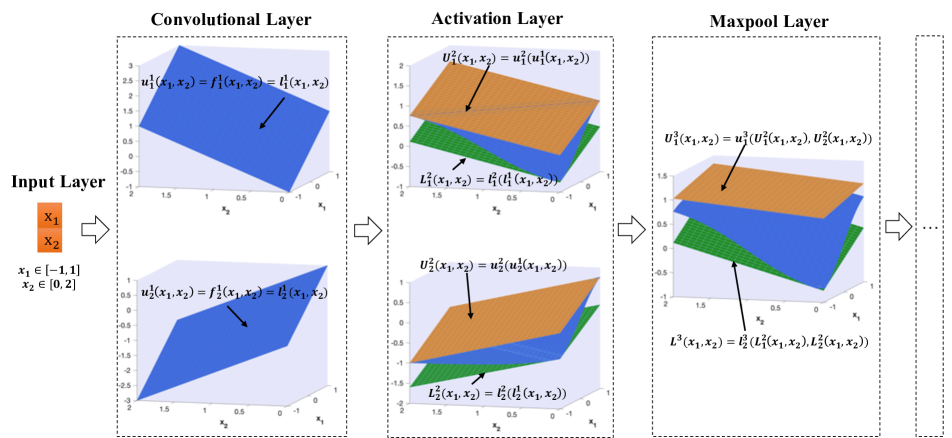
Figure 1: A toy example of MaxLin linear approximation. To simplify, the input size is two, and the perturbation radius is one. $l^{k}_{i}(x^{k}_{i})$ and $u_{i}^{k}(x^{k}_{i})$ are the lower and upper linear bounds of the output of the $i$-th neuron($x^{k}_{i}$) in the $k$-th layer, respectively. $L^{k}_{i}(x_{1},x_{2})$ and $U_{i}^{k}(x_{1},x_{2})$ are the global lower and upper linear bounds of the output of the $i$-th neuron in the $k$-th layer, respectively. The blue surface is the output of the current neuron, and the activation function here is the Tanh function.

To address the above challenges, in this work, we propose MaxLin, an efficient and tight verification framework for MaxPool-based networks via tightening linear approximation. Specifically, to tighten linear approximation, we minimize the maximum value of the upper linear bound and minimize the average precision loss of the lower linear bound of MaxPool. We also prove that our proposed upper bound is block-wise tightest. Compared with existing neuron-wise tightness, our method acheives better certified results. Further, based on single-neuron relaxation, MaxLin gives the linear bounds directly after choosing the first and second maximum values of the upper and lower bound of the MaxPool’s input. Thus, MaxLin has high computation efficiency. A simple example of MaxLin’s computation process is shown in Figure 1. Moreover, MaxLin easily integrates with state-of-the-art verifiers, e.g., CNN-Cert [4], 3DCertify [27], and $\alpha,\beta$-CROWN [48, 41]. The integration allows MaxLin to certify different types of MaxPool-based networks (e.g., CNNs or PointNet) with various activation functions (e.g., Sigmoid, Artan, Tanh or ReLU) against $l_{1},l_{2},l_{\infty}$-norm perturbations.

We evaluate MaxLin with open-sourced benchmarks on the MNIST [24], CIFAR-10 [23], and Tiny ImageNet [11] datasets. The experiment results show that MaxLin outperforms the state-of-the-art techniques including CNN-Cert [4], DeepPoly [37], 3DCertify [27], and Ti-Lin [45] with up to 110.60%, 62.17%, 39.94%, and 49.26% improvement in terms of tightness, respectively. MaxLin has higher efficiency with up to 5.13$\times$ speedup than 3DCertify and comparable efficiency as CNN-Cert, DeepPoly, and Ti-Lin. Further, we compare MaxLin with branch and bound (BaB) methods, including $\alpha$,$\beta$-CROWN [48, 41, 50], ERAN and MN-BaB [12], on ERAN benchmarks. The results show that MaxLin has much higher certified accuracy and less time cost across different perturbation ranges.

In summary, our work proposes an incomplete robustness verification technique, MaxLin, with tighter linear approximation and better efficiency, which works for various CNNs and $l_{p}$-norm perturbations. By tightening linear approximation for MaxPool, our approach outperforms the state-of-the-art tools with up to 110.60% improvement to the certified robustness bounds and up to 5.13$\times$ speedup.

2 Related Work

We now introduce some topics closely related to robustness verification and then introduce other related robustness verification techniques.

2.1 Adversarial Attacks and Defenses

Many research studies [39, 15, 9, 8, 7, 36, 42] show machine learning models are vulnerable to adversarial examples. Adversarial examples pose severe concerns for the deployment of machine learning models in security and safety-critical applications such as autonomous driving. To defend against adversarial examples, many defenses [15, 29, 20, 21, 10, 19, 43, 48, 41, 28] were proposed. Empirical defenses [35, 5] cannot provide a formal robustness guarantee and they are often broken by adaptive, unseen attacks [6, 1, 14]. Thus, we study certified defenses in this work. In particular, we focus on MaxPool-based convolutional neural networks which are widely used for image classification.

2.2 Robustness Verification for MaxPool-based CNNs

As MaxPool is hard to verify, only a few research on robustness verification takes MaxPool into consideration. Recently, a survey on certified defense is proposed [30]. Verification approaches are usually divided into two classes: complete verification and incomplete verification.

As for complete verifiers, Marabou [21] extends Reluplex [20] and proposes a precise SMT-based verification framework to verify arbitrary piece-wise linear network, including ReLU-based networks with MaxPool layers. However, this complete method cannot apply to other non-linear functions, such as Sigmoid and Tanh. Recently, PRIMA [33] proposes a general verification framework based on multi-neuron relaxation and can apply to MaxPool-based networks. Further, MN-BaB [12] proposes a complete neural network verifier that builds on the tight multi-neuron constraints proposed in PRIMA. However, multi-neuron relaxation methods may contain an exponential number of linear constraints at the worst case [40] and cannot verify large models in a feasible time(one day per input) [25].

To break the scalability barrier of the above work and accelerate the verification process, linear approximation based on single-neuron relaxation has been created. CNN-Cert [4] proposes an efficient verification framework with non-trivial linear bounds for MaxPool. However, CNN-Cert is loose in terms of tightness and only applies to layered CNNs and ResNet. DeepPoly [37] proposes a versatile verification framework for different networks. However, it certifies very loose robustness bounds and certifies robustness only against $l_{\infty}$ perturbation form. Recently, 3DCertify propose a novel verifier built atop DeepPoly and can certify the robustness of PointNet. 3DCertify uses the Double Description method to tighten the linear approximation for MaxPool. However, its linear approximation is still loose and it is time-consuming. Ti-Lin [45] proposes the neuron-wise tightest linear bounds for MaxPool by producing the smallest over-approximation zone. However, MaxPool often comes after ReLU, Sigmoid, or other non-linear layers, which pose a big challenge to tighten and thus, Ti-Lin is still loose in tightness.

3 Preliminaries

This section introduces the minimal necessary background of our approach.

3.1 MaxPool-based Neural Networks

We focus on certifying the robustness of MaxPool-based networks for classification tasks. Our methods can refine the abstraction of the MaxPool function in arbitrary networks. For simplicity, we formally use $F:\mathbb{R}^{n_{0}}\to\mathbb{R}^{n_{K}}$ to represent a neural network classifier with (K+1) layers and $F=f^{K}\circ f^{K-1}\circ\cdots f^{2}\circ f^{1}$. Here $f^{1}:\mathbb{R}^{n_{0}}\to\mathbb{R}^{n_{1}},\cdots,f^{K}:\mathbb{R}^{n_{K-1}}\to\mathbb{R}^{n_{K}}$. The symbol $f^{i},i=1,\cdots,K$ could be an affine, activation, fully connected, or MaxPool function. In this work, the non-linear block in neural architectures could be activation or activation+MaxPool. The MaxPool function is defined as follows.

$$MaxPool(x_{i_{1}},\cdots,x_{i_{n}})=max\{x_{i_{1}},\cdots,x_{i_{n}}\}$$

where $i_{1},\cdots,i_{n}$ are the indexes of the input that will be pooled associated with the $i$-th output of the current layer.

As for other notations used in our approach, $n_{k}$ represents the number of neurons in the $k$-th layer and $[K]$ represents the set $\{1,\cdots,K\}$. $F_{j}^{k}(\boldsymbol{x}):\mathbb{R}^{n_{0}}\to\mathbb{R}$ to denote the $j$-th output of the $k$-th layer and $\boldsymbol{x^{k-1}}$ to denote the input of the $k$-th layer.

3.2 Robustness Verification For Neural Networks

Robustness verification aims to find the minimal adversarial attack range. In other words, robustness verification can give the largest certified robustness bound, within which there exist no adversarial examples around the original input. Such the maximum absolute safe radius is defined as local robustness bound $\epsilon_{r}$, which are the formal robustness guarantees provided by complete verifiers.

Define $\boldsymbol{x_{0}}$ be an input data point. Let $\mathbb{B}_{p}(\boldsymbol{x_{0}},\epsilon)$ denotes $\boldsymbol{x_{0}}$ perturbed within an $l_{p}$-normed ball with radius $\epsilon$, that is $\mathbb{B}_{p}(\boldsymbol{x_{0}},\epsilon)=\{\boldsymbol{x}|\|\boldsymbol{x}-\boldsymbol{x_{0}}\|_{p}\leq\epsilon\}$. We focus on $l_{1},l_{2}$, and $l_{\infty}$ adversary, i.e. $p=1,2,\infty$. Let $t$ denote the true label of $\boldsymbol{x_{0}}$. Then local robustness bound is defined as follows.

Definition 1 (Local robustness bound).

$F$ is a neural network and $\epsilon_{r}\geq 0$. $\epsilon_{r}$ is called as the local robustness bound of the input $\boldsymbol{x_{0}}$ in the neural network $F$ if $(\mathop{\arg\max}\limits_{i}F_{i}(\boldsymbol{x})=t,\forall\boldsymbol{x}\in\mathbb{B}_{p}(\boldsymbol{x_{0}},\epsilon_{r}))$ $\wedge$ $(\forall\delta>0,\exists\boldsymbol{x_{a}}\in\mathbb{B}_{p}(\boldsymbol{x_{0}},\epsilon+\delta)s.t.\mathop{\arg\max}\limits_{i}F_{i}(\boldsymbol{x_{a}})\neq t)$.

It is of vital importance to certify local robustness bound for networks. However, it is an NP-complete problem for the simple ReLU-based fully-connected networks [20] and computationally expensive with the worse case of exponential time complexity [30]. Therefore, it is practical to lose some precision to certify a lower bound than $\epsilon_{r}$, which is provided by incomplete verifiers.

Definition 2 (Certified lower bound).

$F$ is a neural network and $\epsilon_{l}\geq 0$. $\epsilon_{l}$ is called as a certified lower bound of the input $\boldsymbol{x_{0}}$ in the neural network $F$ if $(\epsilon_{l}<\epsilon_{r})$ $\wedge$ $(\mathop{\arg\max}\limits_{i}F_{i}(\boldsymbol{x})=t,\forall\boldsymbol{x}\in\mathbb{B}_{p}(\boldsymbol{x_{0}},\epsilon_{l}))$.

Because incomplete verifier risks precision loss to gain scalability and efficiency, the value of $\epsilon_{l}$ becomes a key criterion to evaluate the tightness of robustness verification methods and is used as the metric for tightness in our approach.

3.3 Linear Approximation

Define $\boldsymbol{l^{k-1}},\boldsymbol{u^{k-1}}$ are the lower and upper bound of the input of the $k$-th layer, that is, $\boldsymbol{x^{k-1}}\in[\boldsymbol{l^{k-1}},\boldsymbol{u^{k-1}}]$. The essence of linear approximation technique is giving linear bounds to every layer, that is $\forall k\in[K]$, $l^{k}(\boldsymbol{x^{k-1}})\leq f^{k}(\boldsymbol{x^{k-1}})\leq u^{k}(\boldsymbol{x^{k-1}}),\forall\boldsymbol{x^{k-1}}\in[\boldsymbol{l^{k-1}},\boldsymbol{u^{k-1}}]$.

Definition 3 (Upper/Lower linear bounds).

Let $s^{i}$ be the input associated with the the $i$-th neuron ouput and $f^{k}_{i}(\boldsymbol{s^{i,k-1}})$ be the function of the $i$-th neuron in the $k$-th layer of neural network $F$. With $\boldsymbol{x^{k-1}}\in[\boldsymbol{l^{k-1}},\boldsymbol{u^{k-1}}]\subset\mathbb{R}^{n_{k-1}},$ if $\boldsymbol{s^{i,k-1}}\subset\mathbb{R}^{n}$ and there exists $\boldsymbol{a^{k}_{u}},\boldsymbol{a^{k}_{l}}\in\mathbb{R}^{n}$ and $\boldsymbol{b^{k}_{u}},\boldsymbol{b^{k}_{l}}\in\mathbb{R}$ such that $\forall\boldsymbol{s^{i,k-1}}\subset\boldsymbol{x^{k-1}}\in[\boldsymbol{\boldsymbol{l^{k-1}}},\boldsymbol{u^{k-1}}]$,

$$u^{k}_{i}(\boldsymbol{s^{i,k-1}})=\boldsymbol{a^{k}_{u}}\boldsymbol{s^{i,k-1}}+\boldsymbol{b^{k}_{u}},l^{k}_{i}(\boldsymbol{x^{k-1}})=\boldsymbol{a^{k}_{l}}\boldsymbol{s^{i,k-1}}+\boldsymbol{b^{k}_{l}}$$

$$l^{k}_{i}(\boldsymbol{s^{i,k-1}})\leq f^{k}_{i}(\boldsymbol{s^{i,k-1}})\leq u^{k}_{i}(\boldsymbol{s^{i,k-1}})$$

then, $u^{k}_{i}(\boldsymbol{s^{i,k-1}})$ and $l^{k}_{i}(\boldsymbol{s^{i,k-1}})$ are called upper and lower linear bounds of $f^{k}_{i}(\boldsymbol{s^{i,k-1}})$, respectively.

It is worth mentioning that $n$ is determined by the type of $f^{k}_{i}(\boldsymbol{s^{i,k-1}})$. When $f^{k}_{i}(\boldsymbol{s^{i,k-1}})$ is a univariate function(such as ReLU, Sigmoid, Tanh, or Arctan), $n=1$. When $f^{k}_{i}(\boldsymbol{s^{i,k-1}})$ is a multivariate function, $n$ is equal to the dimension of $\boldsymbol{s^{i,k-1}}$. For example, when $f^{k}_{i}(\boldsymbol{s^{i,k-1}})$ is MaxPool, $n$ is equal to the size of the input to be pooled; When the $k$-th layer is a convolutional layer, $n$ corresponds to the size of the weight filter, and the linear constraints are

$$u^{k}(\boldsymbol{s^{i,k-1}})=\boldsymbol{w}*\boldsymbol{s^{i,k-1}}+\boldsymbol{b},l^{k}(\boldsymbol{s^{i,k-1}})=\boldsymbol{w}*\boldsymbol{s^{i,k-1}}+\boldsymbol{b}$$

where $*$ is the convolution operation. $\boldsymbol{w}$ and $\boldsymbol{b}$ are the filter’s weights and biases, respectively. When the $k$-th layer is a fully-connected layer, $n=n_{k-1}$ and the linear constraints are

$$u^{k}(\boldsymbol{x^{k-1}})=\boldsymbol{w}\boldsymbol{s^{i,k-1}}+\boldsymbol{b},l^{k}(\boldsymbol{s^{i,k-1}})=\boldsymbol{w}\boldsymbol{s^{i,k-1}}+\boldsymbol{b}$$

where $\boldsymbol{w}$ and $\boldsymbol{b}$ are the weights and biases assosicated with the $i$-th ouput neuron in the fully-connected layer, respectively.

After giving linear constraints to the predecessor layers, we can compute the global linear bounds of the current layer, which is represented as:

$$L^{k}(\boldsymbol{x^{0}}):=\boldsymbol{A^{k}_{l}}\boldsymbol{x^{0}}+\boldsymbol{B_{l}^{k}},U^{k}(\boldsymbol{x^{0}}):=\boldsymbol{A^{k}_{u}}\boldsymbol{x^{0}}+\boldsymbol{B_{u}^{k}}$$

where $L^{k}(\boldsymbol{x^{0}})\leq F^{k}(\boldsymbol{x^{0}})\leq U^{k}(\boldsymbol{x^{0}}),\forall\boldsymbol{x^{0}}\in\mathbb{B}_{p}(\boldsymbol{x_{0}},\epsilon)$. The whole procedure is a layer-by-layer process from the first hidden layer to the last output layer, and we can compute a certified lower bound after we get the global linear bounds of the output layer.

4 MaxLin: A Robustness Verifier for MaxPool-based CNNs

In this section, we present MaxLin, a tight and efficient robustness verifier for MaxPool-based networks.

4.1 Tightening Linear Approximation for MaxPool

In this subsection, we propose our MaxPool linear bounds. We use $f(x_{1},\cdots,x_{n})=max\{x_{1},\cdots,x_{n}\}$ to represent the MaxPool function without loss of generality.

Theorem 1.

Given $f(x_{1},\cdots,x_{n})=max\{x_{1},\cdots,x_{n}\}$, $x_{i}\in[l_{i},u_{i}]$, we select the first and the second maximum values of the set $\{u_{i}|i=1,\cdots,n\}$ and assume their indexs are $i,j$, respectively. We use $l_{max}$ to denote the maximum value of the set $\{l_{i}|i=1,\cdots,n\}$. Define $\boldsymbol{m}=(m_{1},\cdots,m_{n})=(\frac{u_{1}+l_{1}}{2},\cdots,\frac{u_{n}+l_{n}}{2})\in\mathbb{R}^{n}$. Then, the linear bounds of the MaxPool function are:

Upper linear bound:

$u(x_{1},\cdots,x_{n}):=\sum_{i}a_{i}(x_{i}-l_{i})+b$. Specifically, there are two different cases:

Case 1: If $(l_{i}=l_{max})\wedge(l_{i}\geq u_{j})$, $a_{i}=1;b=l_{i};a_{k}=0,\forall k\neq i$.

Case 2: Otherwise, $a_{i}=\frac{u_{i}-u_{j}}{u_{i}-l_{i}};b=u_{j};a_{k}=0,\forall k\neq i$.

Lower linear bound:

$l(x_{1},\cdots,x_{n})=x_{j},j=\mathop{\arg\max}\limits_{i}(m_{i})$.

4.2 Block-wise Tightest Property

Existing methods [37, 4, 22, 19, 45] give the neuron-wise tightest linear bounds, producing the smallest the over-approximation zone for the ReLU, Sigmoid, Sigmoid($x$)Tanh($y$),$x$$\cdot$Sigmoid($y$) and MaxPool functions, respectively. This notion ignores the interleavings of neurons and leads to non-optimal results. In this paper, we introduce the notion of block-wise tightest, that is, the volume of the over-approximation zone between the global linear bounds of the ReLU+MaxPool block is the minimum. This notion considers the interleavings of neurons, and the achieved results will be superior to existing neuron-wise tightest. Without loss of generality, we assume Activation is at the $k$-th layer, and we use $U^{k+1}_{b}(\cdot)$ and $L^{k+1}_{b}(\cdot)$ to denote the global upper and lower linear bounds of the Activation+MaxPool block, respectively. Then, we define the notion of block-wise tightest as follows:

Definition 4 (Block-wise Tightest).

The global linear bounds of the Activation+MaxPool block are $U^{k+1}_{b}(\boldsymbol{x^{k}})$ and $L^{k+1}_{b}(\boldsymbol{x^{k}})$, respectively. Then, we define $U^{k+1}_{b}(\boldsymbol{x^{k}})$ and $L^{k+1}_{b}(\boldsymbol{x^{k}})$ is the block-wise tightest if and only if $\iint_{\boldsymbol{x^{k-1}}\in[\boldsymbol{l^{k-1},\boldsymbol{u^{k-1}]}}}(U^{k+1}_{b}(\boldsymbol{x^{k-1}})-L^{k+1}_{b}(\boldsymbol{x^{k-1}}))d\boldsymbol{x^{k-1}}$ reach the minimum.

Furthermore, if the non-linear block is ReLU+MaxPool and the abstraction for ReLU is not precise and instead uses the neuron-wise tightest upper linear bound, then MaxLin has the provably block-wise tightest upper linear bound.

Theorem 2.

If the preceding layer of the MaxPool function is ReLU with $u(x)=\frac{u}{u-l}(x-l)$ as the upper linear bound [4, 37, 48], the upper linear bound in Theorem 1 is the block-wise tightest.

We put the proofs of Theorem 1 and Theorem 2 in the supplementary material.

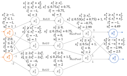
Figure 2: A toy example of how MaxLin computing global bounds $\boldsymbol{l^{K}}$ and $\boldsymbol{u^{K}}$ against $l_{\infty}$ adversary. The first, second, third, and fourth hidden layers are the affine, ReLU, MaxPool, and affine functions, respectively.

4.3 Computing Certified Lower Bounds

The whole process of computing certified lower bounds can be divided into two parts: (i) computing the global upper and lower bounds $\boldsymbol{l^{K}},\boldsymbol{u^{K}}$ of the network output $F^{K}(\boldsymbol{x})$ and (ii) searching the maximal certified lower bound.

4.3.1 Computing the global upper and lower bounds $\boldsymbol{l^{K}},\boldsymbol{u^{K}}$ of the network output $F^{K}(\boldsymbol{x})$

Given a certain perturbation range $\epsilon$ and an original input $\boldsymbol{x_{0}}$, MaxLin can tightly compute the global upper and lower bounds $\boldsymbol{l^{K}},\boldsymbol{u^{K}}$ of the network output $F^{K}(\boldsymbol{x})$ to check whether $\epsilon$ is a certified safe perturbation radius or not.

This process starts at a basic step, that is, we give a pair of linear bounds with the input range $\mathbb{B}_{p}(\boldsymbol{x_{0}},\epsilon)$ of $f^{1}(\boldsymbol{x})$, and then with $k=1$, we compute $\boldsymbol{l^{1}}$, $\boldsymbol{u^{1}}$ based on Equation (1) which are deduced [43] by Holder’s inequality.

$$F^{k}(\boldsymbol{x})\leq\epsilon\|\boldsymbol{A^{k}_{u}}\|_{q}+\boldsymbol{A^{k}_{u}}\boldsymbol{x_{0}}+\boldsymbol{B^{k}_{u}},$$ (1)

$$F^{k}(\boldsymbol{x})\geq-\epsilon\|\boldsymbol{A^{k}_{l}}\|_{q}+\boldsymbol{A^{k}_{l}}\boldsymbol{x_{0}}+\boldsymbol{B^{k}_{l}}$$

where $\|\cdot\|_{q}$ is $l_{q}$ norm and $\frac{1}{p}+\frac{1}{q}=1$. In our work, we focus on $l_{1},l_{2},l_{\infty}$-norm adversary and thus, $p=1,2,\infty$.

In the second step, without loss of generality, we assume the current layer is the $k$-th layer. Given $\boldsymbol{l^{k-1}},\boldsymbol{u^{k-1}}$, we give upper and lower linear bounds $u^{k}(\boldsymbol{x}),l^{k}(\boldsymbol{x})$, respectively. Then, we use Equation (1) to attain $\boldsymbol{l^{k}},\boldsymbol{u^{k}}$ by backsubstitution [37], which we will illustrate in detail later. $k$ in the second step can be all positive integers that are smaller than $K$. Repeating the second step from $k=2$ to $k=K$, we can get the value of $\boldsymbol{l^{K}}$ and $\boldsymbol{u^{K}}$. If $l^{K}_{t}\geq u^{K}_{j},\forall j\neq t,j\in[n_{K}]$, $\epsilon$ is a certified safe perturbation radius. Otherwise, $\epsilon$ cannot be certified to be a safe perturbation radius.

A toy example. To better illustrate the process of backsubstitution, we give a toy example of how we compute $\boldsymbol{l^{K}}$ and $\boldsymbol{u^{K}}$ of a five-layer fully-connected network, whose biases are zero(see Figure 2). The $i$-th neuron at the $k$-th layer is represented as $x^{k}_{i}$ and the perturbed input is within $\mathbb{B}_{\infty}([0,1]^{T},1)$. The input layer(orange) and the output layer(blue) both have two nodes, and the MaxPool function is a bivariate function for simplicity. In this example, $x^{4}_{1}$ is the output neuron of the true label.

Concretely, We get the value of $u^{4}_{2}$ by backsubstitution:

$$x^{4}_{2} \leq-x_{1}^{3}+x_{2}^{3}$$

$$\leq-x_{1}^{2}+0.5x_{3}^{2}+1$$

$$\leq-x_{1}^{1}+0.5(0.25x_{3}^{1}+1.5)+1$$

$$\leq-x_{1}^{0}-x_{2}^{0}+0.5(0.25(2x_{1}^{0}-2x_{2}^{0})+1.5)+1$$

$$\leq-0.75x_{1}^{0}-1.25x_{2}^{0}+1.75$$

$$\leq 2.5$$

Therefore, $u^{4}_{2}=2.5$. We get $l^{4}_{1}=-1,u^{4}_{1}=4.49,l^{4}_{2}=-2.99$ similarly. $u^{4}_{2}\geq l^{4}_{1}$ means that $\epsilon=1$ is not a certified safe perturbation range, and we need to decrease $\epsilon$ to find the maximal robustness lower bound that we could certify.

Algorithm 1 Computing certified lower bound

0:  model F, input $\boldsymbol{x}$, true label $t$;

0:  $\epsilon_{l}$;

1:  Let $\epsilon_{0}\leftarrow 0.005$,$\epsilon_{l}\leftarrow\epsilon_{0},\epsilon_{min}\leftarrow 0,\epsilon_{max}\leftarrow 1$.

2:  for i=0 to 14 do

3:     Compute $\boldsymbol{l^{K}},\boldsymbol{u^{K}}$ of $F(\boldsymbol{x})$, where $\boldsymbol{x}\in\mathbb{B}_{p}(\boldsymbol{x_{0}},\epsilon_{l})$

4:     if $l^{K}_{t}\geq max_{j\neq t}(u^{K}_{j})$ then

5:        $\epsilon_{min}=\epsilon_{l}$

6:        $\epsilon_{l}=min(2\epsilon_{l},\frac{\epsilon_{max}+\epsilon_{min}}{2})$;

7:     else

8:        $\epsilon_{max}=\epsilon_{l}$

9:        $\epsilon_{l}=max(\frac{\epsilon_{l}}{2},\frac{\epsilon_{max}+\epsilon_{min}}{2})$;

10:     end if

11:  end for

12:  return  $\epsilon_{l}$

4.3.2 Computing maximal certified lower bound $\epsilon_{l}$

We use the binary search algorithm to find the maximal certified lower bound, which is the certified lower bound results in our work (see Algorithm 1). To make sure the perturbation range is larger than zero, we decrease or increase the perturbation range (lines 1, 6, and 9). When the perturbation range is certified safe (line 4), we then increase $\epsilon$ (line 6); When $\epsilon$ cannot be certified safe, we then decrease $\epsilon$ (line 9). The difference between $\epsilon_{max}$ and $\epsilon_{min}$ is already reasonably small ($\leq 2^{-15}$) after the process is repeated 15 times. Finally, after the above checking process is repeated 15 times, the algorithm will terminate and return $\epsilon_{l}$ as the certified lower bound results. For a K-layer convolutional network, if we assume that the $k$-th layer has $n_{k}$ neurons and the filter size is $k\times k$, the time complexity of MaxLin is $\mathcal{O}(K^{2}\times\max{n_{k}}^{3})$. Detailed analysis are in the Appendix.

5 Experimental Evaluation

Table 1: Averaged certified lower bounds and runtime on CNNs on MNIST, CIFAR-10, and Tiny ImageNet datasets tested by CNN-Cert, Ti-Lin, and MaxLin.

Dataset	Network		Certified Bounds($\boldsymbol{10^{-5}}$)			Bound Improvement(%)		Average Runtime(min)
		$\boldsymbol{l_{p}}$	CNN-Cert	Ti-Lin	MaxLin	vs. CNN-Cert	vs. Ti-Lin	CNN-Cert	Ti-Lin	MaxLin
MNIST	CNN	$l_{\infty}$	1318	1837	2083	58.04$\uparrow$	13.39$\uparrow$	1.76	1.73	1.37
	4 layers	$l_{2}$	4427	6478	7131	61.08$\uparrow$	10.08$\uparrow$	1.39	1.38	1.40
	36584 nodes	$l_{1}$	8544	12642	13808	61.61$\uparrow$	9.22$\uparrow$	1.38	1.38	1.50
	CNN	$l_{\infty}$	1288	1817	2712	110.60$\uparrow$	49.26$\uparrow$	8.44	8.76	7.82
	5 layers	$l_{2}$	5164	7359	9987	93.40$\uparrow$	35.71$\uparrow$	11.90	9.18	7.47
	52872 nodes	$l_{1}$	10147	14292	19000	87.25$\uparrow$	32.94$\uparrow$	10.77	9.46	7.70
	CNN	$l_{\infty}$	1025	1382	1942	89.46$\uparrow$	40.52$\uparrow$	20.46	20.87	15.90
	6 layers	$l_{2}$	3954	5409	6981	76.56$\uparrow$	29.06$\uparrow$	20.56	20.41	15.94
	56392 nodes	$l_{1}$	7708	10455	13218	71.48$\uparrow$	26.43$\uparrow$	20.60	20.01	15.93
	CNN	$l_{\infty}$	647	930	1289	99.23$\uparrow$	38.60$\uparrow$	24.71	24.55	18.91
	7 layers	$l_{2}$	2733	4022	5228	91.29$\uparrow$	29.99$\uparrow$	25.08	23.80	18.92
	56592 nodes	$l_{1}$	5443	8002	10248	88.28$\uparrow$	28.07$\uparrow$	22.86	22.87	18.78
	CNN	$l_{\infty}$	847	1221	1666	96.69$\uparrow$	36.45$\uparrow$	26.51	26.66	22.19
	8 layers	$l_{2}$	3751	5320	6641	77.05$\uparrow$	24.83$\uparrow$	25.01	24.85	22.01
	56912 nodes	$l_{1}$	7515	10655	12897	71.62$\uparrow$	21.04$\uparrow$	23.72	24.23	22.27
	LeNet_ReLU	$l_{\infty}$	1204	1864	2093	73.83$\uparrow$	12.29$\uparrow$	0.16	0.17	0.17
	3 layers	$l_{2}$	6534	10862	11750	79.83$\uparrow$	8.18$\uparrow$	0.16	0.17	0.17
	8080 nodes	$l_{1}$	17937	30305	32313	80.15$\uparrow$	6.63$\uparrow$	0.16	0.17	0.17
	LeNet_Sigmoid	$l_{\infty}$	1684	2042	2567	52.43$\uparrow$	25.71$\uparrow$	0.26	0.28	0.27
	3 layers	$l_{2}$	9926	12369	14535	46.43$\uparrow$	17.51$\uparrow$	0.27	0.27	0.27
	8080 nodes	$l_{1}$	26937	33384	38264	42.05$\uparrow$	14.62$\uparrow$	0.27	0.27	0.27
	LeNet_Tanh	$l_{\infty}$	613	817	943	53.83$\uparrow$	15.42$\uparrow$	0.27	0.27	0.27
	3 layers	$l_{2}$	3462	4916	5424	56.67$\uparrow$	10.33$\uparrow$	0.27	0.27	0.27
	8080 nodes	$l_{1}$	9566	13672	14931	56.08$\uparrow$	9.21$\uparrow$	0.27	0.27	0.27
	LeNet_Atan	$l_{\infty}$	617	836	961	55.75$\uparrow$	14.95$\uparrow$	0.26	0.27	0.27
	3 layers	$l_{2}$	3514	5010	5517	57.00$\uparrow$	10.12$\uparrow$	0.28	0.27	0.27
	8080 nodes	$l_{1}$	9330	13345	14522	55.65$\uparrow$	8.82$\uparrow$	0.27	0.28	0.27
CIFAR-10	CNN	$l_{\infty}$	108	129	147	36.11$\uparrow$	13.95$\uparrow$	3.09	2.92	2.94
	4 layers	$l_{2}$	751	1038	1172	56.06$\uparrow$	12.91$\uparrow$	2.47	2.51	2.50
	49320 nodes	$l_{1}$	2127	3029	3392	59.47$\uparrow$	11.98$\uparrow$	2.46	2.48	2.49
	CNN	$l_{\infty}$	115	146	169	46.96$\uparrow$	15.75$\uparrow$	13.10	13.04	13.07
	5 layers	$l_{2}$	953	1342	1519	59.39$\uparrow$	13.19$\uparrow$	12.39	12.69	12.61
	71880 nodes	$l_{1}$	2850	4087	4582	60.77$\uparrow$	12.11$\uparrow$	12.34	12.61	12.51
	CNN	$l_{\infty}$	99	120	139	40.40$\uparrow$	15.83$\uparrow$	28.56	28.63	28.61
	6 layers	$l_{2}$	830	1078	1217	46.63$\uparrow$	12.89$\uparrow$	27.63	27.89	27.49
	77576 nodes	$l_{1}$	2387	3174	3558	49.06$\uparrow$	12.10$\uparrow$	27.66	27.36	27.68
	CNN	$l_{\infty}$	66	83	96	45.45$\uparrow$	15.66$\uparrow$	33.37	33.27	33.44
	7 layers	$l_{2}$	573	773	889	55.15$\uparrow$	15.01$\uparrow$	32.48	32.77	32.42
	77776 nodes	$l_{1}$	1673	2303	2623	56.78$\uparrow$	13.89$\uparrow$	33.56	32.55	32.96
	CNN	$l_{\infty}$	56	70	85	51.79$\uparrow$	21.43$\uparrow$	36.86	37.54	37.64
	8 layers	$l_{2}$	536	705	835	55.78$\uparrow$	18.44$\uparrow$	37.46	36.59	36.91
	78416 nodes	$l_{1}$	1609	2160	2532	57.36$\uparrow$	17.22$\uparrow$	36.89	37.01	37.38
Tiny ImageNet	CNN	$l_{\infty}$	77	123	128	66.23$\uparrow$	4.07$\uparrow$	184.94	183.98	185.81
	7 layers	$l_{2}$	580	939	962	65.86$\uparrow$	2.45$\uparrow$	184.36	183.25	185.07
	703512 nodes	$l_{1}$	1747	2875	2934	67.95$\uparrow$	2.05$\uparrow$	193.62	183.93	184.03

In this section, we conduct extensive experiments on CNNs by comparing MaxLin with four state-of-the-art backsubstitution-based tools (CNN-Cert [4], DeepPoly [37], 3DCertify [27], and Ti-Lin [45]). Further, we compare MaxLin with BaB and multi-neuron abstraction tools ($\alpha$,$\beta$-CROWN [48, 41, 50], ERAN and MN-BaB [12]). The experiments run on a server running a 48 core Intel Xeon Silver 4310 CPU and 125 GB of RAM.

5.1 Experimental Setup

Framework. The linear bounds of MaxLin are independent of the concrete verifier, and thus, we instantiate CNN-Cert [4] and 3DCertify [27] verifiers with MaxLin to certify the robustness of CNNs. Concretely, CNN-Cert verifier is the state-of-the-art verification framework and can support the $l_{1},l_{2},l_{\infty}$ perturbation form, while 3DCertify verifier is built atop ERAN framework and can certify various networks against $l_{\infty}$ perturbation and other perturbation forms (such as rotation).

Linear bounds for activations. As for the linear approximation of activations, we choose linear bounds in VeriNet [19] as our Sigmoid/Tanh/Arctan’s linear bounds. Further, we choose linear bounds in DeepPoly [37] as our ReLU’s linear bounds. These linear bounds are all the provable neuron-wise tightest [51] and stand for the highest precision among other relevant work [30]. It is noticeable that when we compare MaxLin to other tools, only the linear bounds for MaxPool are different for a fair comparison, that is, both the linear bounds of the activation functions and the other experiment setup are the same.

Datasets. Our experiments are conducted on MNIST, CIFAR-10, and Tiny ImageNet, the well-known image datasets. The MNIST [24] is a dataset of $28\times 28$ handwritten digital images in 10 classes(from 0 to 9). CIFAR-10 [23] is a dataset of 60,000 $32\times 32\times 3$ images in 10 classes. Tiny ImageNet [11] consists of 100,000 $64\times 64\times 3$ images in 200 classes. The value of each pixel is normalized into [0,1] and thus, the perturbation radius is in [0,1].

Benchmarks. We evaluate the performance of MaxLin on two classes of maxpool-based networks: (I) CNNs, whose activation function is the ReLU function and with Batch Normalization; (II) LeNet, whose activation function is the Sigmoid, tanh, or arctan function. The networks used in experiments are all open-sourced and come from ERAN and CNN-Cert.

Metrics. We refer to the metrics in CNN-Cert. As for tightness, we use $\frac{100(\epsilon_{l}^{\prime}-\epsilon_{l})}{\epsilon_{l}}\%$ to quantify the percentage of improvement, where $\epsilon_{l}^{\prime}$ and $\epsilon_{l}$ represent the average certified lower bounds certified by MaxLin and other comparative tools, respectively. As for efficiency, we record the average computation time over the correctly-classified images and use $\frac{t}{t^{\prime}}$ to represent the speedup of MaxLin over other baseline methods, where $t$ and $t^{\prime}$ are the average computation time of MaxLin and other tools, respectively. Some detailed experiment setups are in the Appendix.

5.2 Performance on CNN-Cert

As both MaxLin and Ti-Lin are built upon CNN-Cert, the state-of-the-art verification framework, we compare MaxLin to CNN-Cert and Ti-Lin. The generation way of the test set is the same as CNN-Cert, which generates 10 test images randomly.

As for the tightness, MaxLin outperforms CNN-Cert and Ti-Lin in all settings with up to 110.60% and 49.26% improvement in Table 1, respectively. The reason why MaxLin outperforms Ti-Lin, the neuron-wise tightest technique, is that minimizing the over-approximation zone is more effective for a single non-linear layer, whose nearest predecessor and posterior layers are linear. The MaxPool layer is usually placed after the activation layer and thus, Ti-Lin is inferior to MaxLin. As for time efficiency, as they share the same verification framework, CNN-Cert, and they can directly give linear bounds for MaxPool, the time cost of these three methods is almost the same.

5.3 Performance on ERAN

As MaxLin, DeepPoly, and 3DCertify are built upon the ERAN framework, which only can verify robustness against the $l_{\infty}$ adversary, we compare MaxLin with DeepPoly and 3DCertify atop ERAN framework. CNNs with 4, 5, and 6 layers are from CNN-Cert, and CNNs with 7 and 8 layers are not supported by ERAN due to some undefined operations in the networks. MNIST_LeNet_Arctan is not used in this experiment as ERAN does not support arctan. Furthermore, ERAN does not support Tiny ImageNet either. The generation way of the test set is the same as ERAN, which chooses the first 10 images to test tools.

As for tightness, MaxLin outperforms DeepPoly and 3DCertify with up to 62.17% and 39.94% improvement in Table 2, respectively. MaxLin computes much tighter certified lower bounds than 3DCertify in most cases, and the only bad result of MaxLin only occurs in MNIST_LeNet_Sigmoid when compared with 3DCertify. This is reasonable. As the weights and biases of networks are quite different from each other, which makes the performance of verifiers varies on different networks as discussed in [51]. However, we argue that MaxLin outperforms existing SOTA verifiers on MaxPool-based networks as MaxLin computes larger certified lower bounds in most cases.

Table 2: Averaged certified lower bounds and runtime on CNNs on the MNIST and CIFAR-10 datasets tested by DeepPoly, 3DCertify, and MaxLin.

Dataset	Network	Certified Bounds($\mathbf{10^{-6}}$)			Bound Improvement(%)		Average Runtime(min)			Speedup
		DeepPoly	3DCertify	MaxLin	vs. DeepPoly	vs. 3DCertify	DeepPoly	3DCertify	MaxLin	vs. 3DCertify
MNIST	Conv_Maxpool	2802	3247	4544	62.17$\uparrow$	39.94$\uparrow$	0.54	1.21	0.58	2.09
	CNN, 4 layers	9375	10621	11272	20.23$\uparrow$	6.13$\uparrow$	1.34	4.44	1.48	3.01
	CNN, 5 layers	6642	7629	7948	19.66$\uparrow$	4.18$\uparrow$	5.40	13.13	5.51	2.38
	CNN, 6 layers	6339	7325	7554	19.17$\uparrow$	3.13$\uparrow$	11.88	27.87	12.47	2.23
	LeNet_ReLU	8849	10937	11225	26.85$\uparrow$	2.63$\uparrow$	0.14	0.69	0.19	3.70
	LeNet_Sigmoid	12122	14716	14506	19.67$\uparrow$	-1.43$\downarrow$	0.15	1.01	0.20	5.13
	LeNet_Tanh	2966	3637	3675	23.90$\uparrow$	1.04$\uparrow$	0.17	0.82	0.19	4.31
CIFAR-10	Conv_Maxpool	661	725	754	14.07$\uparrow$	4.00$\uparrow$	8.16	9.84	8.35	1.18
	CNN, 4 layers	1204	1460	1542	28.07$\uparrow$	5.62$\uparrow$	2.64	4.25	2.64	1.61
	CNN, 5 layers	1223	1537	1579	29.11$\uparrow$	2.73$\uparrow$	11.82	17.75	12.44	1.43
	CNN, 6 layers	1065	1415	1440	35.21$\uparrow$	1.77$\uparrow$	24.60	40.44	24.89	1.62

As for time efficiency, 3DCertify is quite time-consuming as it tries to find the best upper linear bound from the linear bounds set gained by the Double Description Method [13]. However, MaxLin can give the upper and lower linear bounds directly after choosing the first and second maximum values of the upper and lower bound of maxpool’s input $\boldsymbol{l}$ and $\boldsymbol{u}$ and thus, is efficient. Therefore, MaxLin has up to 5.13$\times$ speedup compared with 3DCertify and almost the same time efficiency as DeepPoly in Table 2.

5.4 Evaluating The Block-wise Tightness

To further illustrate the superiority of the block-wise tightness, we compare MaxLin and the baselines by the volume of the Activation+MaxPool block. The pool size is $2\times 2$, and the number of inputs is 50. The Activation has three types: (i) ReLU, whose linear bounds are the provably neuron-wise tightest [37, 49]; (ii) Adaptive-ReLU [48], whose upper linear bounds is $u(x)=\frac{ReLU(u)-ReLU(l)}{u-l}$ and lower linear bounds is adaptive: $l(x)=ax,a\in[0,1]$; (iii) Sigmoid, whose linear bounds are the provably neuron-wise tightest [19]. Specifically, we employ a random sampling approach to determine both the upper and lower bounds for each pixel, following a uniform distribution $U(-10,10)$. Simultaneously, we randomly select the value of $a$ from a uniform distribution $U(0,1)$.

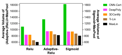
Figure 3: The average volume of the Activation+MaxPool block computed by CNN-Cert, DeepPoly, 3DCertify, Ti-Lin and MaxLin.

Figure 3 shows the average volume of the Activation+MaxPool block computed by the baselines and MaxLin. Concretely, MaxLin has the smallest volume of the over-approximation zone of the ReLU+MaxPool and Adaptive-ReLU+MaxPool blocks among the baseline methods, which validates the correctness of Theorem 2. Further, in terms of S-shaped activation functions, MaxLin has the smallest results regarding the average volume. This shows that when the upper linear bound is not the provably block-wise tightest, MaxLin can also reduce the over-approximation zone of the non-linear block. Moreover, The results show that the neuron-wise tightest linear bounds (Ti-Lin) could only keep high precsion through one layer, while MaxLin could keep the tightness through one-block propagation. The results in Figure 3 are consistent with the results in Table 1 and 2 and indicate the advantage of the block-wise tightest upper linear bound in terms of precision.

5.5 Additional Experiments

We conduct additional experiments to further demonstrate the superiority and broad applicability of MaxLin. The detailed settings are in the Appendix, and we perform the following experiments: (I) We compare the output interval $[\boldsymbol{l^{K}},\boldsymbol{u^{K}}]$ computed by MaxLin and Ti-Lin to further illstrates the advantages of the block-wise tightness over the neuron-wise tightness. (II) We conduct extensive experiments by comparing the time efficiency of BaB-based and backsubstitution-based verification frameworks. (III) We compare MaxLin with BaB-based verification frameworks, including VNN-COMP 2021-2023 [2, 32] winner $\alpha$,$\beta$-CROWN [48, 41, 50], ERAN using multi-neuron abstraction and MN-BaB [12] on ERAN benchmark. (IV) We also conduct experiments by certifying the robustness of PointNet on the ModelNet40 dataset [44] to illustrate the broad applicability of MaxLin.

6 Conclusion

In this paper, we propose MaxLin, a tight linear approximation approach to MaxPool for computing larger certified lower bounds for CNNs. MaxLin has high execution efficiency as it uses the single-neuron relaxation technique and computes linear bounds with low computational consumption. MaxLin is built atop CNN-Cert and 3DCertify, two state-of-the-art verification frameworks, and thus, can certify the robustness of various networks(e.g., CNNs and PointNet) with arbitrary activation functions against $l_{1},l_{2},l_{\infty}$ perturbation form. We evaluate MaxLin with open-sourced benchmarks on the MNIST, CIFAR-10, and Tiny ImageNet datasets. The results show that MaxLin outperforms the SOTA tools with at most 110.60% improvement regarding the certified lower bound and 5.13 $\times$ speedup for the same neural networks.

7 Appendix

7.1 Experiment Setups

In this subsection, we present some experiment setups in detail. Concretely, we list the sources of networks, the size of the test set, and the initial perturbation range in Table 3. We evaluate methods on 10 inputs for all CNNs in Table 1 and 2. As CIFAR_Conv_MaxPool has low accuracy and low robustness, the size of the test set is 50 and the initial perturbation range is 0.00005. Testing on 10 inputs can sufficiently evaluate the performance of verification methods, as it is shown that the average certified results of 1000 inputs are similar to 10 images [4].

7.2 Additional Experiments

In this subsection, we conduct some additional experiments to further illustrate (I) the advantage of the block-wise tighness over the neuron-wise tightness, (II) the time efficiency of MaxLin compared to other BaB-based verification tools, (III) the performance of MaxLin using multi-neuron abstraction techniques, and (IV) the performance of MaxLin on PointNets.

We list the sources of networks for additional experiments in Table 3. We evaluate methods on 100 inputs for ERAN benchmark (CIFAR_Conv_MaxPool) and 100 inputs for PointNets. The perturbation range $\epsilon$ is 0.005 for PointNets and is 0.0007, 0.0008, 0.0009, 0.0010, or 0.0011 for CIFAR_Conv_MaxPool. We follow the metrics used in the baseline methods. As for the effectiveness, we use certified accuracy, the percentage of the successfully verified inputs against the perturbation range, to evaluate the tightness of methods. We also use the average per-example verified time as the metric for time efficiency. In additional experiments II and III, we compare MaxLin with three state-of-the-art verification techniques, which use the BaB and multi-neuron abstraction technique to enhance the precision. Concretely, the baselines are MN-BaB [12], $\alpha$,$\beta$-CROWN [48, 41, 50] (VNN-COMP 2021 [2] and 2022 [32] winner), and ERAN. In additional experiment IV, we evaluate the performance of MaxLin and three single-neuron abstraction methods(DeepPoly [37], 3DCertify [27], and Ti-Lin [45]) on PointNets.

Table 3: The additional experimental setup and source of neural networks used in experiments. $\epsilon_{0}$ is the initial perturbation range in Algorithm 1. The third column represents the size of the input test set.

Dataset	Network	Size	$\boldsymbol{\epsilon_{0}}$	Source
MNIST	Conv_MaxPool	10	0.005	ERAN
	CNN, 4 layers	10	0.005	CNN-Cert
	CNN, 5 layers	10	0.005
	CNN, 6 layers	10	0.005
	CNN, 7 layers	10	0.005
	CNN, 8 layers	10	0.005
	LeNet_ReLU	10	0.005
	LeNet_Sigmoid	10	0.005
	LeNet_Tanh	10	0.005
	LeNet_Atan	10	0.005
CIFAR-10	Conv_MaxPool	50	0.00005	ERAN
	CNN, 4 layers	10	0.005	CNN-Cert
	CNN, 5 layers	10	0.005
	CNN, 6 layers	10	0.005
	CNN, 7 layers	10	0.005
	CNN, 8 layers	10	0.005
Tiny ImageNet	CNN, 7 layers	10	0.005
ModelNet40	16p_natural	100	0.005	3DCertify
	32p_natural	100	0.005
	64p_natural	100	0.005
	128p_natural	100	0.005
	256p_natural	100	0.005

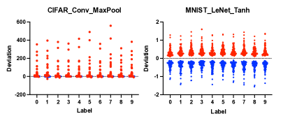
Figure 4: Visualization of the output intervals verified by MaxLin and Ti-Lin. $(\boldsymbol{l},\boldsymbol{u})$ and $(\boldsymbol{l^{\prime}},\boldsymbol{u^{\prime}})$ represent the output bound of Ti-Lin and MaxLin testing on 100 inputs, respectively. Red and blue dots represent $\boldsymbol{u}-\boldsymbol{u^{\prime}}$ and $\boldsymbol{l}-\boldsymbol{l^{\prime}}$, respectively.

7.2.1 Results (I): Advantages Over The Neuron-wise Tightest Method

To further illustrate the advantage of the block-wise tightness (MaxLin) over the neuron-wise tightness(Ti-Lin), we analyze the verified interval of the output neurons of the last layer. In Figure 4, we compare the results computed by MaxLin and Ti-Lin on CIFAR_Conv_MaxPool and MNIST_LeNet_Tanh, whose actvations are ReLU and S-shaped, respectively. For the output neurons(10 labels), we use $(\boldsymbol{l},\boldsymbol{u})$ and $(\boldsymbol{l^{\prime}},\boldsymbol{u^{\prime}})$ to represent the output bound of Ti-Lin and MaxLin testing on 100 inputs, respectively. We use the red and blue dots to represent $\boldsymbol{u}-\boldsymbol{u^{\prime}}$ and $\boldsymbol{l}-\boldsymbol{l^{\prime}}$, respectively. The $x$-axis represents the output neuron index(label), and the $y$-axis represents the deviations between the lower and upper bounds of the intervals.

As the activation of CIFAR_Conv_MaxPool is ReLU, the lower bounds of the ouput neurons are mostly zero and thus the deviation of lower bounds is zero. Except for this case, most $u-u^{\prime}$ are larger than zero and $l-l^{\prime}$ are smaller than zero in Figure 4. It reveals that the block-wise tightest upper linear bounds could bring tighter output intervals than the neuron-wise tightest linear bounds. Consequently, MaxLin could certify much larger robustness bounds than Ti-Lin in Table 1.

7.2.2 Results (II): Performance Using Single-neuron Abstraction for ReLU

We conduct additional experiments to present the time efficiency of the single-neuron abstraction technique, which is used by MaxLin in Section 5. We compare MaxLin(single-neuron abstraction for ReLU) with three state-of-the-art verification techniques(MN-BaB [12], $\alpha$,$\beta$-CROWN [48, 41], and ERAN using multi-neuron abstraction) on CIFAR_Conv_MaxPool. The results are presented in Figure 5. In terms of time efficiency, MaxLin can accelerate the computation process with up to $14.1,96.5,$ and $23.8\times$ compared to MN-BaB, $\alpha,\beta$-CROWN, and ERAN, respectively. Although MaxLin uses the single-neuron abstraction technique for ReLU, MaxLin still can enhance precision with up to 9.1, 9.1, and 3.0% improvement compared to MN-BaB, $\alpha,\beta$-CROWN, and ERAN , respectively. These results demonstrate that the single-neuron abstraction technique has the potential of verifying large models and other complex models, such as PointNets(results in Subsection 7.2.4)

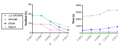
Figure 5: Certified accuracy(%) and average per-example verification time(s) on CIFAR_Conv_MaxPool tested by MN-BaB, $\alpha$,$\beta$-CROWN, ERAN, and MaxLin(using single-neuron techniques for ReLU).

7.2.3 Results (III): Performance Using Multi-neuron Abstraction for ReLU

As ERAN framework, atop which MaxLin is built, not only supports single-neuron abstraction but also integrates the multi-neuron abstraction for ReLU. We compare MaxLin using multi-neuron abstraction for ReLU to MN-BaB, $\alpha$, $\beta$-CROWN, and ERAN using multi-neuron abstraction on CIFAR_Conv_MaxPool. The results are shown in Figure 6. The results show that MaxLin has higher certified accuracy with up to 15.2, 15.2, 6.1% improvement compared to MN-BaB, $\alpha$, $\beta$-CROWN, and ERAN, respectively. In terms of time efficiency, MaxLin has similar time cost to MN-BaB and has up to 9.5 and 1.9 $\times$ speedup compared to $\alpha$, $\beta$-CROWN and ERAN, respectively. These results show that if using multi-neuron abstraction, MaxLin also could have higher certified accuracy and less time cost than these verification tools.

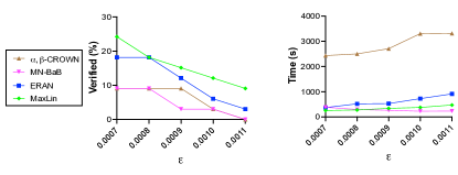
Figure 6: Certified accuracy(%) and average per-example verification time(s) on CIFAR_Conv_MaxPool tested by MN-BaB, $\alpha$,$\beta$-CROWN, ERAN, and MaxLin(using multi-neuron techniques for ReLU).

Table 4: Averaged certified results and runtime on PointNet on the ModelNet40 datasets tested by DeepPoly, 3DCertify, Ti-Lin, and MaxLin, where 16p_natural represents the PointNet model is naturally trained and the number of its point input is 16.

Dataset	Network	Certified accuracy (%)				Average Runtime(second)				Speedup
		DeepPoly	3DCertify	Ti-Lin	MaxLin	DeepPoly	3DCertify	Ti-Lin	MaxLin	vs. 3DCertify
ModelNet40	16p_natural	72.73	74.03	74.03	74.03	10.37	18.22	12.47	10.61	1.72
	32p_natural	54.88	58.54	58.54	64.63	17.88	34.79	21.24	18.06	1.93
	64p_natural	32.56	40.70	36.05	47.67	35.85	96.04	42.96	36.63	2.62
	128p_natural	4.55	11.36	2.27	14.77	81.46	207.04	110.16	85.90	2.41
	256p_natural	1.12	4.49	1.12	4.49	178.34	494.70	248.19	199.88	2.47

7.2.4 Results (IV): Performance on PointNets

3D point cloud models are widely used and achieve great success in some safety-critical domains, such as autonomous driving. It is of vital importance to provide a provable robustness guarantee to models before deployed.

As 3DCertify is a robustness verifier for point cloud models, MaxLin, which is built atop the 3DCertify framework, can be extended to certify the robustness of 3D Point Cloud models against point-wise $l_{\infty}$ perturbation and 3D transformation. Here, we demonstrate that MaxLin is not only useful beyond image classification models but also performs well on other models. To that end, we show certification results against point-wise $l_{\infty}$ perturbation on seven PointNets for the ModelNet40 [44] dataset in Table 4. The PointNet whose inputs’ point number is $k$ is denoted as $k$p_natural. As Ti-Lin is the best state-of-the-art tool built on the CNN-Cert framework, we integrate its linear bounds for MaxPool into the 3DCertify framework as one baseline. The generation way of the test set is the same as 3DCertify and all experiments use the same random subset of 100 objects from the ModelNet40 [44] dataset. The certification results represent the percentage of verified robustness properties and the perturbation range is 0.005. The perturbation is in $l_{\infty}$ norm and is measured by Hausdroff distance.

As for tightness, the certification results in Table 4 show that MaxLin outperforms other tools in all cases in terms of tightness. It is reasonable that the results for 16p_natural and 256_natural certified by 3DCertify and MaxLin are the same, as the perturbation range is not large enough to distinguish the tightness of these tools. As for efficiency, in Table 4, MaxLin has up to 2.62 $\times$ speedup compared with 3DCertify and is slightly faster than Ti-Lin. MaxLin has almost the same time consumption as DeepPoly. In summary, these results demonstrate that our fine-grained linear approximation can help improve both the tightness and efficiency of robustness verification of other models beyond the image classification domain.

7.3 Complexity analysis of MaxLin

For a K-layer convolutional network, we assume that the $k$-th layer has $n_{k}$ neurons and the filter size is $k\times k$. The time complexity of backsubstitution is $\mathcal{O}(K\times\max n_{k}^{3})$ [49] and the backsubstitution process will be repeated $K-1$ times to verify one input perturbed within a certain perturbation range. Therefore, the time complexity of MaxLin is $\mathcal{O}(K^{2}\times\max{n_{k}}^{3})$.

7.4 Proof of Theorem 1

We prove the correctness of linear bounds in Theorem 1 as follows.

Proof.

Upper linear bound:

Case 1:

When $(l_{i}=l_{max})\wedge(l_{i}\geq u_{j})$, $u(x_{1},\cdots,x_{n})=x_{i}$ and $f(x_{1},\cdots,x_{n})=x_{i}$. Therefore,

$$u(x_{1},\cdots,x_{n})-f(x_{1},\cdots,x_{n})= x_{i}-x_{i}$$

$$= 0$$

Case 2:

Otherwise, $f(x_{1},\cdots,x_{n})=max\{x_{1},\cdots,x_{n}\}$

If $f(x_{1},\cdots,x_{n})=x_{i}$,

$$u(x_{1},\cdots,x_{n})-f(x_{1},\cdots,x_{n})$$

$$= \frac{u_{i}-u_{j}}{u_{i}-l_{i}}(x_{i}-l_{i})+u_{j}-x_{i}$$

$$= \frac{l_{i}-u_{j}}{u_{i}-l_{i}}x_{i}-\frac{u_{j}-l_{i}}{u_{i}-l_{i}}u_{i}$$

$$= \frac{u_{j}-l_{i}}{u_{i}-l_{i}}(u_{i}-x_{i})$$

$$\geq 0$$

If $f(x_{1},\cdots,x_{n})=x_{j}$,

$$u(x_{1},\cdots,x_{n})-f(x_{1},\cdots,x_{n})$$

$$= \frac{u_{i}-u_{j}}{u_{i}-l_{i}}(x_{i}-l_{i})+u_{j}-x_{j}$$

$$\geq 0$$

Otherwise, we assume $f(x_{1},\cdots,x_{n})=x_{q}$, where $q\neq i,j$ and $q\in[n]$.

$$u(x_{1},\cdots,x_{n})-f(x_{1},\cdots,x_{n})$$

$$= \frac{u_{i}-u_{j}}{u_{i}-l_{i}}(x_{i}-l_{i})+u_{j}-x_{q}$$

$$\geq \frac{u_{i}-u_{j}}{u_{i}-l_{i}}(x_{i}-l_{i})+u_{j}-u_{q}$$

$$\geq 0$$

Lower linear bound:

$$f(x_{1},\cdots,x_{n})= max(x_{1},\cdots,x_{n})$$

$$\geq x_{j}$$

$$= l(x_{1},\cdots,x_{n})$$

This completes the proof. ∎

7.5 Proof of Theorem 2

First, we prove minimizing the volume of the over-approximation zone of the linear bounds $U^{k+1}_{b}(\cdot)$ and $L^{k+1}_{b}(\cdot)$ for non-linear block is equivalent to minimizing $U^{k+1}_{b}(m^{k-1})$ and $L^{k+1}_{b}(m^{k-1})$, respectively.

Theorem 3.

Minimizing

$$\iint_{\boldsymbol{x^{k-1}}\in[\boldsymbol{l^{k-1},\boldsymbol{u^{k-1}]}}}(U^{k+1}_{b}(\boldsymbol{x^{k-1}})-L^{k+1}_{b}(\boldsymbol{x^{k-1}}))d\boldsymbol{x^{k-1}}$$

is equivalent to minimizing $U^{k+1}_{b}(\boldsymbol{m^{k-1}})$ and $L^{k+1}_{b}(\boldsymbol{m^{k-1}})$

The proof of Theorem 3 is as follows.

Proof.

First, Minimizing

$$\iint_{\boldsymbol{x^{k-1}}\in[\boldsymbol{l^{k-1},\boldsymbol{u^{k-1}]}}}(U^{k+1}_{b}(\boldsymbol{x^{k-1}})-L^{k+1}_{b}(\boldsymbol{x^{k-1}}))d\boldsymbol{x^{k-1}}$$

is equivalent to minimizing the

$$\iint_{\boldsymbol{x^{k-1}}\in[\boldsymbol{l^{k-1},\boldsymbol{u^{k-1}]}}}(U^{k+1}_{b}(\boldsymbol{x^{k-1}})-f^{k-1}(\boldsymbol{x^{k-1}}))d\boldsymbol{x^{k-1}}$$

and

$$\iint_{\boldsymbol{x^{k-1}}\in[\boldsymbol{l^{k-1},\boldsymbol{u^{k-1}]}}}(f^{k-1}(\boldsymbol{x^{k-1}})-L^{k+1}_{b}(\boldsymbol{x^{k-1}}))d\boldsymbol{x^{k-1}}$$

, respectively.

Therefore, it is equivalent to minimize the $\iint_{\boldsymbol{x^{k-1}}\in[\boldsymbol{l^{k-1},\boldsymbol{u^{k-1}]}}}U^{k+1}_{b}(\boldsymbol{x^{k-1}})d\boldsymbol{x^{k-1}}$ and $\iint_{\boldsymbol{x^{k-1}}\in[\boldsymbol{l^{k-1},\boldsymbol{u^{k-1}]}}}(-L^{k+1}_{b}(\boldsymbol{x^{k-1}}))d\boldsymbol{x^{k-1}}$, respectively.

Because $U^{k+1}_{b}(\boldsymbol{x^{k-1}})$ is a linear combination of $\boldsymbol{x^{k-1}}$. Without loss of generality, we assume $U^{k+1}_{b}(\boldsymbol{x^{k-1}})=\sum_{q\in[n_{k-1}]}A_{u,q}^{k+1}x_{q}^{k-1}+B^{k+1}_{u}$. Then,

$$\iint_{\boldsymbol{x}\in[\boldsymbol{l^{k-1}},\boldsymbol{u^{k-1}}]}U^{k+1}_{b}(\boldsymbol{x^{k-1}})d\boldsymbol{x}$$

$$= \iint_{\boldsymbol{x}\in[\boldsymbol{l^{k-1}},\boldsymbol{u^{k-1}}]}(\sum_{q\in[n_{k-1}]}A_{u,q}^{k+1}x_{q}+B^{k+1}_{u})d\boldsymbol{x}$$

$$= \Pi_{i=1}^{n_{k-1}}(u^{k-1}_{i}-l^{k-1}_{i})(\sum_{q\in[n_{k-1}]}A_{u,q}^{k+1}\frac{u^{k-1}_{q}+l^{k-1}_{q}}{2}+B^{k+1}_{u})$$

$$= \Pi_{i=1}^{n_{k-1}}(u^{k-1}_{i}-l^{k-1}_{i})U_{b}^{k+1}(\boldsymbol{m^{k-1}})$$

where $\boldsymbol{m^{k-1}}=(\frac{u^{k-1}_{1}+l^{k-1}_{1}}{2},\cdots,\frac{u^{k-1}_{n_{k-1}}+l^{k-1}_{n_{k-1}}}{2})$, because $u^{k-1}_{q},l^{k-1}_{q}$, $q\in[n_{k-1}]$ are constant, and the minimize target has been transformed into minimizing $U_{b}^{k+1}(\boldsymbol{m})$.

Therefore, minimizing $\iint_{\boldsymbol{x^{k-1}}\in[\boldsymbol{l^{k-1},\boldsymbol{u^{k-1}]}}}U^{k+1}_{b}(\boldsymbol{x^{k-1}})$ is equivalent to minimize $U^{k+1}_{b}(\boldsymbol{m^{k-1}})$

Similarly, minimizing $-\iint_{\boldsymbol{x^{k-1}}\in[\boldsymbol{l^{k-1},\boldsymbol{u^{k-1}]}}}L^{k+1}_{b}(\boldsymbol{x^{k-1}})$ is equivalent to minimize $-L^{k+1}_{b}(\boldsymbol{m^{k-1}})$ ∎

Based on Theorem 3, we prove Theorem 2 as follows.

Proof.

When $l<0\wedge u>0$, the linear bounds of ReLU used in our approach are the same as [37, 49, 4], which are the provable neuron-wise tightest upper linear bounds [37]. It is:

$$u(x)=\frac{u}{u-l}(x-l)$$ (2)

First, we prove the upper linear bound is the block-wise tightest. Without loss of generality, we assume ReLU is at the $k$-th layer. We use $u^{k+1},l^{k+1}$ and $u_{M}^{k+1},l_{M}^{k+1}$ to denote other linear bounds and our linear bounds for the MaxPool function, respectively. As the slope of the MaxPool linear bounds is always non-negative, the global upper and lower linear bounds of the ReLU+MaxPool block are:

$$u^{k+1}(x^{k}_{1},\cdots,x^{k}_{n})$$

$$\leq u^{k+1}(u^{k}(x^{k-1}_{1}),\cdots,u^{k}(x^{k-1}_{n}))$$

$$=: U^{k+1}_{b}(x^{k-1}_{1},\cdots,x^{k-1}_{n})$$

$$l^{k+1}(x^{k}_{1},\cdots,x^{k}_{n})$$

$$\leq l^{k+1}(l^{k}(x^{k-1}_{1}),\cdots,l^{k}(x^{k-1}_{n}))$$

$$=: L^{k+1}_{b}(x^{k-1}_{1},\cdots,x^{k-1}_{n})$$

where we use $U^{k+1}_{b}(\cdot)$ and $L_{b}^{k+1}(\cdot)$ to denote the global upper and lower linear bounds of the ReLU+MaxPool block, respectively.

If $U^{k+1}_{b}(m^{k-1}_{1},\cdots,m^{k-1}_{n})$ reaches its minimum, the upper linear bound of Theorem 1 are the provable block-wise tightest.

Upper linear bound:

$$U^{k+1}_{b}(m^{k-1}_{1},\cdots,m^{k-1}_{n})$$

$$= u^{k+1}(u^{k}(m^{k-1}_{1}),\cdots,u^{k}(m^{k-1}_{n}))$$

$$= u^{k+1}(\frac{u^{k-1}_{1}(m^{k-1}_{1}-l^{k-1}_{1})}{u^{k-1}_{1}-l^{k-1}_{1}},\cdots,\frac{u^{k-1}_{n}(m^{k-1}_{n}-l^{k-1}_{n})}{u^{k-1}_{n}-l^{k-1}_{n}})$$

$$= u^{k+1}(\frac{u^{k-1}_{1}(\frac{u^{k-1}_{1}-l^{k-1}_{1}}{2})}{u^{k-1}_{1}-l^{k-1}_{1}},\cdots,\frac{u^{k-1}_{n}(\frac{u^{k-1}_{1}-l^{k-1}_{1}}{2})}{u^{k-1}_{n}-l^{k-1}_{n}})$$

$$= u^{k+1}(\frac{u^{k-1}_{1}}{2},\cdots,\frac{u^{k-1}_{n}}{2})$$

$$= \frac{1}{2}u^{k+1}({u^{k-1}_{1}},\cdots,{u^{k-1}_{n}})$$

$$= \frac{1}{2}u^{k+1}({u^{k}_{1}},\cdots,{u^{k}_{n}})$$

$$\geq \frac{1}{2}max\{u^{k}_{1},\cdots,u^{k}_{n}\}$$

$$= \frac{1}{2}u_{M}^{k+1}({u^{k}_{1}},\cdots,{u^{k}_{n}})$$

This means $u_{M}^{k+1}(\cdot)$ is the block-wise tightest. ∎

References

- Athalye et al. [2018] Anish Athalye, Nicholas Carlini, and David Wagner. Obfuscated gradients give a false sense of security: Circumventing defenses to adversarial examples. In International conference on machine learning (ICML), pages 274–283, 2018.
- Bak et al. [2021] Stanley Bak, Changliu Liu, and Taylor Johnson. The second international verification of neural networks competition (vnn-comp 2021): Summary and results. arXiv preprint arXiv:2109.00498, 2021.
- Balunovic et al. [2019] Mislav Balunovic, Maximilian Baader, Gagandeep Singh, Timon Gehr, and Martin Vechev. Certifying geometric robustness of neural networks. Advances in Neural Information Processing Systems (NeurIPS), 32:1–11, 2019.
- Boopathy et al. [2019] Akhilan Boopathy, Tsui-Wei Weng, Pin-Yu Chen, Sijia Liu, and Luca Daniel. Cnn-cert: an efficient framework for certifying robustness of convolutional neural networks. In Proceedings of the AAAI Conference on Artificial Intelligence (AAAI), pages 3240–3247, 2019.
- Buckman et al. [2018] Jacob Buckman, Aurko Roy, Colin Raffel, and Ian Goodfellow. Thermometer encoding: One hot way to resist adversarial examples. In International conference on learning representations (ICLR), 2018.
- Carlini and Wagner [2017a] Nicholas Carlini and David Wagner. Adversarial examples are not easily detected: Bypassing ten detection methods. In Proceedings of the 10th ACM workshop on artificial intelligence and security, pages 3–14, 2017a.
- Carlini and Wagner [2017b] Nicholas Carlini and David Wagner. Towards evaluating the robustness of neural networks. In IEEE S & P, pages 39–57, 2017b.
- Chen et al. [2020] Jianbo Chen, Michael I Jordan, and Martin J Wainwright. Hopskipjumpattack: A query-efficient decision-based attack. In IEEE S & P, pages 1277–1294, 2020.
- Chen et al. [2017] Pin-Yu Chen, Huan Zhang, Yash Sharma, Jinfeng Yi, and Cho-Jui Hsieh. Zoo: Zeroth order optimization based black-box attacks to deep neural networks without training substitute models. In Proceedings of the 10th ACM workshop on artificial intelligence and security, pages 15–26, 2017.
- Cohen et al. [2019] Jeremy Cohen, Elan Rosenfeld, and Zico Kolter. Certified adversarial robustness via randomized smoothing. In International conference on machine learning (ICML), pages 1310–1320, 2019.
- Deng et al. [2009] Jia Deng, Wei Dong, Richard Socher, Li-Jia Li, Kai Li, and Li Fei-Fei. Imagenet: A large-scale hierarchical image database. In IEEE Conference on Computer Vision and Pattern Recognition (CVPR), pages 248–255, 2009.
- Ferrari et al. [2022] Claudio Ferrari, Mark Niklas Muller, Nikola Jovanovic, and Martin Vechev. Complete verification via multi-neuron relaxation guided branch-and-bound. arXiv preprint arXiv:2205.00263, pages 1–15, 2022.
- Fukuda and Prodon [2005] Komei Fukuda and Alain Prodon. Double description method revisited. In Combinatorics and Computer Science, pages 91–111, 2005.
- Ghiasi et al. [2020] Amin Ghiasi, Ali Shafahi, and Tom Goldstein. Breaking certified defenses: Semantic adversarial examples with spoofed robustness certificates. arXiv preprint arXiv:2003.08937, pages 1–16, 2020.
- Goodfellow et al. [2014] Ian J Goodfellow, Jonathon Shlens, and Christian Szegedy. Explaining and harnessing adversarial examples. arXiv preprint arXiv:1412.6572, 2014.
- Gopinath et al. [2018] Divya Gopinath, Guy Katz, Corina S Păsăreanu, and Clark Barrett. Deepsafe: a data-driven approach for assessing robustness of neural networks. In International symposium on automated technology for verification and analysis (ATVA), pages 3–19, 2018.
- Goswami et al. [2018] Gaurav Goswami, Nalini Ratha, Akshay Agarwal, Richa Singh, and Mayank Vatsa. Unravelling robustness of deep learning based face recognition against adversarial attacks. In Proceedings of the AAAI Conference on Artificial Intelligence (AAAI), pages 1–10, 2018.
- He et al. [2016] Kaiming He, Xiangyu Zhang, Shaoqing Ren, and Jian Sun. Deep residual learning for image recognition. In Proceedings of the IEEE conference on computer vision and pattern recognition (CVPR), pages 770–778, 2016.
- Henriksen and Lomuscio [2020] Patrick Henriksen and Alessio Lomuscio. Efficient neural network verification via adaptive refinement and adversarial search. In European Conference on Artificial Intelligence (ECAI), pages 2513–2520, 2020.
- Katz et al. [2017] Guy Katz, Clark Barrett, David L Dill, Kyle Julian, and Mykel J Kochenderfer. Reluplex: an efficient smt solver for verifying deep neural networks. In International Conference on Computer Aided Verification (CAV), pages 97–117, 2017.
- Katz et al. [2019] Guy Katz, Derek A Huang, Duligur Ibeling, Kyle Julian, Christopher Lazarus, Rachel Lim, Parth Shah, Shantanu Thakoor, Haoze Wu, Aleksandar Zeljić, et al. The marabou framework for verification and analysis of deep neural networks. In International Conference on Computer Aided Verification(CAV), pages 443–452, 2019.
- Ko et al. [2019] Ching-Yun Ko, Zhaoyang Lyu, Lily Weng, Luca Daniel, Ngai Wong, and Dahua Lin. Popqorn: quantifying robustness of recurrent neural networks. In International Conference on Machine Learning (ICML), pages 3468–3477, 2019.
- Krizhevsky and Hinton [2009] A. Krizhevsky and G. Hinton. Learning multiple layers of features from tiny images. Master’s thesis, Department of Computer Science, University of Toronto, 2009.
- LeCun [1998] Yann LeCun. The mnist database of handwritten digits. http://yann. lecun. com/exdb/mnist/, page 1, 1998.
- Li et al. [2023] Linyi Li, Tao Xie, and Bo Li. Sok: certified robustness for deep neural networks. IEEE Symposium on Security and Privacy (SP), pages 1–23, 2023.
- Liu et al. [2022] Zhuang Liu, Hanzi Mao, Chao-Yuan Wu, Christoph Feichtenhofer, Trevor Darrell, and Saining Xie. A convnet for the 2020s. In Proceedings of the IEEE/CVF conference on computer vision and pattern recognition (CVPR), pages 11976–11986, 2022.
- Lorenz et al. [2021] Tobias Lorenz, Anian Ruoss, Mislav Balunović, Gagandeep Singh, and Martin Vechev. Robustness certification for point cloud models. In Proceedings of the IEEE/CVF International Conference on Computer Vision (ICCV), pages 7608–7618, 2021.
- Lyu et al. [2020] Zhaoyang Lyu, Ching-Yun Ko, Zhifeng Kong, Ngai Wong, Dahua Lin, and Luca Daniel. Fastened crown: tightened neural network robustness certificates. In Proceedings of the AAAI Conference on Artificial Intelligence (AAAI), pages 5037–5044, 2020.
- Madry et al. [2018] Aleksander Madry, Aleksandar Makelov, Ludwig Schmidt, Dimitris Tsipras, and Adrian Vladu. Towards deep learning models resistant to adversarial attacks. In International Conference on Learning Representations (ICLR), 2018.
- Meng et al. [2022] Mark Huasong Meng, Guangdong Bai, Sin Gee Teo, Zhe Hou, Yan Xiao, Yun Lin, and Jin Song Dong. Adversarial robustness of deep neural networks: a survey from a formal verification perspective. IEEE Transactions on Dependable and Secure Computing (TDSC), 1:1–18, 2022.
- Moosavi-Dezfooli et al. [2017] Seyed-Mohsen Moosavi-Dezfooli, Alhussein Fawzi, Omar Fawzi, and Pascal Frossard. Universal adversarial perturbations. In Proceedings of the IEEE conference on computer vision and pattern recognition (CVPR), pages 1765–1773, 2017.
- Müller et al. [2022a] Mark Niklas Müller, Christopher Brix, Stanley Bak, Changliu Liu, and Taylor T Johnson. The third international verification of neural networks competition (vnn-comp 2022): summary and results. arXiv preprint arXiv:2212.10376, 2022a.
- Müller et al. [2022b] Mark Niklas Müller, Gleb Makarchuk, Gagandeep Singh, Markus Püschel, and Martin Vechev. Prima: general and precise neural network certification via scalable convex hull approximations. Proceedings of the ACM on Programming Languages (POPL), pages 1–33, 2022b.
- Nath et al. [2014] Siddhartha Sankar Nath, Girish Mishra, Jajnyaseni Kar, Sayan Chakraborty, and Nilanjan Dey. A survey of image classification methods and techniques. In International conference on control, instrumentation, communication and computational technologies (ICCICCT), pages 554–557, 2014.
- Papernot et al. [2016] Nicolas Papernot, Patrick McDaniel, Xi Wu, Somesh Jha, and Ananthram Swami. Distillation as a defense to adversarial perturbations against deep neural networks. In IEEE S & P, pages 582–597, 2016.
- Silva and Najafirad [2020] Samuel Henrique Silva and Peyman Najafirad. Opportunities and challenges in deep learning adversarial robustness: A survey, 2020.
- Singh et al. [2019a] Gagandeep Singh, Timon Gehr, Markus Püschel, and Martin Vechev. An abstract domain for certifying neural networks. Proceedings of the ACM on Programming Languages (POPL), pages 1–30, 2019a.
- Singh et al. [2019b] Gagandeep Singh, Timon Gehr, Markus Püschel, and Martin Vechev. Boosting robustness certification of neural networks. In International Conference on Learning Representations (ICLR), pages 1–12, 2019b.
- Szegedy et al. [2013] Christian Szegedy, Wojciech Zaremba, Ilya Sutskever, Joan Bruna, Dumitru Erhan, Ian Goodfellow, and Rob Fergus. Intriguing properties of neural networks. arXiv preprint arXiv:1312.6199, pages 1–10, 2013.
- Tjandraatmadja et al. [2020] Christian Tjandraatmadja, Ross Anderson, Joey Huchette, Will Ma, Krunal Kishor Patel, and Juan Pablo Vielma. The convex relaxation barrier, revisited: tightened single-neuron relaxations for neural network verification. Advances in Neural Information Processing Systems (NeurIPS), 33:21675–21686, 2020.
- Wang et al. [2021] Shiqi Wang, Huan Zhang, Kaidi Xu, Xue Lin, Suman Jana, Cho-Jui Hsieh, and J Zico Kolter. Beta-crown: efficient bound propagation with per-neuron split constraints for neural network robustness verification. Advances in Neural Information Processing Systems (NeurIPS), 34:29909–29921, 2021.
- Wu et al. [2023] Baoyuan Wu, Li Liu, Zihao Zhu, Qingshan Liu, Zhaofeng He, and Siwei Lyu. Adversarial machine learning: A systematic survey of backdoor attack, weight attack and adversarial example, 2023.
- Wu and Zhang [2021] Yiting Wu and Min Zhang. Tightening robustness verification of convolutional neural networks with fine-grained linear approximation. In Proceedings of the AAAI Conference on Artificial Intelligence(AAAI), pages 11674–11681, 2021.
- Wu et al. [2015] Zhirong Wu, Shuran Song, Aditya Khosla, Fisher Yu, Linguang Zhang, Xiaoou Tang, and Jianxiong Xiao. 3d shapenets: A deep representation for volumetric shapes. In Proceedings of the IEEE conference on computer vision and pattern recognition (CVPR), pages 1912–1920, 2015.
- Xiao et al. [2022] Yuan Xiao, Tongtong Bai, Mingzheng Gu, Chunrong Fang, and Zhenyu Chen. Certifying robustness of convolutional neural networks with tight linear approximation. arXiv preprint arXiv:2211.09810, pages 1–15, 2022.
- Xie et al. [2017] Saining Xie, Ross Girshick, Piotr Dollár, Zhuowen Tu, and Kaiming He. Aggregated residual transformations for deep neural networks. In Proceedings of the IEEE conference on computer vision and pattern recognition (CVPR), pages 1492–1500, 2017.
- Xiong et al. [2016] Wayne Xiong, Jasha Droppo, Xuedong Huang, Frank Seide, Mike Seltzer, Andreas Stolcke, Dong Yu, and Geoffrey Zweig. Achieving human parity in conversational speech recognition. arXiv preprint arXiv:1610.05256, pages 1–13, 2016.
- Xu et al. [2021] Kaidi Xu, Huan Zhang, Shiqi Wang, Yihan Wang, Suman Jana, Xue Lin, and Cho-Jui Hsieh. Fast and complete: enabling complete neural network verification with rapid and massively parallel incomplete verifiers. International Conference on Learning Representations (ICLR), pages 1–15, 2021.
- Zhang et al. [2018] Huan Zhang, Tsui-Wei Weng, Pin-Yu Chen, Cho-Jui Hsieh, and Luca Daniel. Efficient neural network robustness certification with general activation functions. Advances in Neural Information Processing Systems (NeurIPS), pages 1–10, 2018.
- Zhang et al. [2022a] Huan Zhang, Shiqi Wang, Kaidi Xu, Linyi Li, Bo Li, Suman Jana, Cho-Jui Hsieh, and J Zico Kolter. General cutting planes for bound-propagation-based neural network verification. Advances in Neural Information Processing Systems (NeurIPS), 35:1656–1670, 2022a.
- Zhang et al. [2022b] Zhaodi Zhang, Yiting Wu, Si Liu, Jing Liu, and Min Zhang. Provably tightest linear approximation for robustness verification of sigmoid-like neural networks. In IEEE/ACM International Conference on Automated Software Engineering (ASE), pages 1–13, 2022b.