Effects of local cosmic inhomogeneities on the gravitational wave event rate

Abstract

The local universe is highly inhomogeneous and anisotropic. We live in a relatively sparse region of the Laniakea supercluster at the edge of a large 80 Mpc-wide void. We study the effect of these inhomogeneities on the measured gravitational wave event rates. In particular, we estimate how the measured merger rate of compact binaries is biased by the local matter distribution. The effect of the inhomogeneities on the merger rate is suppressed by the low angular resolution of gravitational wave detectors coupled with their smoothly decreasing population-averaged sensitivity with distance. We estimate the effect on the compact binary coalescence event rate to be at most 6% depending of the chirp mass of the target binary system and the sensitivity and orientation of the detectors.

I Introduction

Detection of gravitational waves (GW) from compact binaries has become routine since their first detection in 2015 Abbott et al. (2016a) by the LIGO Aasi et al. (2015) and Virgo Acernese et al. (2015) collaborations. Since then, around 100 compact binary coalescence (CBC) events have been detected Abbott et al. (2023a) in the first observing runs, and another 80 public alerts in the first part of the fourth observing run LIGO et al. (2023). Most of the events detected so far correspond to massive systems at high redshift, where the distribution of matter in the universe can be well approximated by a homogeneous and isotropic distribution Essick et al. (2023); Vitale et al. (2022). However, when studying the merger rates of systems with smaller masses such as neutron stars (NS) Abbott et al. (2023b) or sub-solar mass (SSM) Abbott et al. (2023c) black holes, the distances explored by the GW detectors is much smaller, in a range where the matter distribution is far from homogeneous.

In fact, we know from local surveys like CosmicFlows-4 Courtois et al. (2023) that the Milky Way galaxy lives in a supercluster called Laniakea Tully et al. (2014); Dupuy and Courtois (2023), moving towards the Great Attractor Dressler et al. (1987) and ”surfing” a large wall surrounding an 80 Mpc wide void. The local universe contains huge cosmic structures such as the Sloan Great Wall Gott et al. (2005), a filament-shaped overdensity located at a distance of $~{}\sim 200$ Mpc and measuring a staggering $\sim 400$ Mpc, challenging previous assumptions of the homogeneity scale of our universe Alonso et al. (2015). Such an inhomogeneous matter distribution must necessarily have an impact on the probability that a given GW event occurs at a given distance in a given direction, assuming that the binary black hole (BBH) progenitors’ location correlates with the matter distribution, i.e. more events towards large concentrations of matter.

The effect of local inhomogeneities may therefore affect our inference of the rate of GW events. By this we mean that we may infer a rate of events which is biased by our location in the universe, which would have to be taken into account when constraining theoretical models, or when extrapolating the measured rates to estimate rates coming from regions which are further away than what has been measured.

In this paper we have studied the effect on the rate of events of the known matter inhomogeneities measured on Ref. Courtois et al. (2023) using the peculiar (i.e., gravitational) velocities of galaxies from the CosmicFlows (CF) catalogs Tully et al. (2016, 2023). We have used the antenna patterns of the two LIGO detectors (Hanford and Livingston) and the Virgo detector, as well as the rotation of the Earth, which sweeps through the sky and further smears out the sensitivity to cosmic matter angular inhomogeneities. Under these assumptions we find that the effect on the sensitive time-volume $\langle VT\rangle$ for a compact binary coalescence (CBC) search is at most 6%.

In Section II we study the VT formalism in an inhomogeneous universe. In Section III we estimate the effect of the local universe inhomogeneities in the rate of BBH events and compute the effect of these inhomogeneities for current GW detectors, and in Section IV we give our conclusions.

A python code to reproduce the results of this paper is publicly available at https://github.com/gmorras/Inhomogeneous_VT.

II The inhomogeneous universe $\langle VT\rangle$

Population analysis and estimation of merger rates of compact binaries rely on the sensitive time-volume ($\langle VT\rangle$) surveyed by the GW searches they are based on. For example, if no event is detected, using loudest event statistics, upper limit constraints on the merger rate can be computed as Biswas et al. (2009)

$$R_{\mathrm{C.L.}}=\frac{-\log(1-C.L.)}{\langle VT\rangle}\,.$$ (1)

where C.L. indicates the confidence level and it is usually chosen to be $\mathrm{C.L.}=90\%$. For a given GW search, the sensitive time-volume surveyed can be measured as

$$\langle VT\rangle\!\!=\!\!\int_{T}\!\!{\rm d}t\!\int_{V}\!\!{\rm d}V_{c}\frac{1}{1+z}\frac{R(\vec{x})}{\overline{R}_{0}}\int\!\!{\rm d}\vec{\theta}\,p_{\mathrm{pop}}(\vec{\theta})\epsilon(\vec{x},t,\vec{\theta})\,,$$ (2)

where the time integral is done in the duration of the search of length $T$, the factor $1/(1+z)$ accounts for the time dilation of the intrinsic rate Abbott et al. (2016b); Tiwari (2018), $R(\vec{x})$ denotes the local event rate at position $\vec{x}$ and $\overline{R}_{0}$ is the average rate at redshift $z=0$. The rate $R(\vec{x})$ depends on position due to both the rate inhomogeneities induced by the inhomogeneities of the universe, as well as due to the evolution of the mean merger rate with cosmic time. For example, in the case of stellar mass BBHs ($m_{\mathrm{BH}}>5M_{\odot}$), there is evidence that, for $z\lesssim 1$, the mean merger rate behaves as Abbott et al. (2023b)

$$\overline{R}^{\mathrm{BBH}}(z)=\overline{R}_{0}^{\mathrm{BBH}}\cdot(1+z)^{\kappa}\,\,\quad\mathrm{with}\;\;\kappa=2.9^{+1.7}_{-1.8}.$$ (3)

In Eq. (2), $\epsilon(\vec{x},t,\vec{\theta})$ denotes the probability to detected a signal with source position $\vec{x}$ and arrival time $t$ as a function of its intrinsic parameters $\vec{\theta}$, and $p_{\mathrm{pop}}(\vec{\theta})$ is the distribution function for the astrophysical population. We can define a time and population averaged probability to detected a signal at position $\vec{x}$ as

$$\epsilon(\vec{x})=\frac{1}{T}\int_{T}{\rm d}t\int{\rm d}\vec{\theta}p_{\mathrm{pop}}(\vec{\theta})\epsilon(\vec{x},t,\vec{\theta})\,.$$ (4)

We also define $\delta_{R}(\vec{x})$ as the event rate inhomogeneities, i.e. the deviations of the event rate $R(\vec{x})$ from its average at the present epoch $\overline{R}_{0}$ as

$$\delta_{R}(\vec{x})=\frac{R(\vec{x})-\overline{R}_{0}}{\overline{R}_{0}}\,,$$ (5)

using Eqs. (4,5) we can rewrite Eq. (2) as

$$\langle VT\rangle=T\int_{V}{\rm d}V_{c}(1+\delta_{R}(\vec{x}))\epsilon(\vec{x})\frac{1}{1+z}\,,$$ (6)

The average probability to detect a signal $\epsilon(\vec{x})$ will depend on its position due to two effects. First of all it will depend on redshift $z$, since the amplitude of the GWs is inversely proportional to the luminosity distance ($h\propto 1/d_{L}(z)$), making it harder to detect them at further distances. It will also depend on the position of the source in the sky, since even though GW detectors usually have broad angular sensitivity, they do not have the same sensitivity in all directions Chen et al. (2017). For earth-bound detectors, if the duration of the search is much longer than a day ($T\gg 1\,\mathrm{day}$), we expect the rotation of the earth to average out the dependence of the sensitivity with right ascension $\alpha$, and therefore to have

$$\epsilon(\vec{x})=\epsilon(z,\delta)\,,$$ (7)

where $\delta$ is the declination of the GW source. In the integral of Eq. (6), the comoving volume element is given by:

$${\rm d}V_{c}=d_{M}^{2}\,{\rm d}d_{c}\,{\rm d}\alpha\,{\rm d}\sin{\delta}$$ (8)

where $d_{c}$ is the comoving distance, defined as

$$d_{c}(z)=\frac{c}{H_{0}}\int_{0}^{z}\frac{{\rm d}z^{\prime}}{E(z^{\prime})}\,,$$ (9)

$E(z)$ is the dimensionless Hubble parameter, defined as

$$E(z)=\frac{H(z)}{H_{0}}$$

$$=\sqrt{\Omega_{r}(1+z)^{4}+\Omega_{m}(1+z)^{3}+\Omega_{k}(1+z)^{2}+\Omega_{\Lambda}}\,,$$ (10)

and in Eq. (8), $d_{M}(z)$ is the comoving transverse distance, defined as

$$d_{M}(z)=\begin{cases}\frac{1}{\sqrt{\Omega_{k}}}\frac{c}{H_{0}}\sinh\left(\sqrt{\Omega_{k}}\frac{H_{0}d_{c}(z)}{c}\right)&\;\Omega_{k}>0\\ d_{c}(z)&\;\Omega_{k}=0\\ \frac{1}{\sqrt{|\Omega_{k}|}}\frac{c}{H_{0}}\sin\left(\sqrt{|\Omega_{k}|}\frac{H_{0}d_{c}(z)}{c}\right)&\;\Omega_{k}<0\end{cases}\,.$$ (11)

III Estimating the effect of the inhomogeneities

III.1 Approximating the efficiency of GW detectors

To estimate the effect of the inhomogeneities, we will assume that we can detect all signals with optimum SNR above a given signal to noise ratio threshold $\rho_{\mathrm{thr}}$

$$\epsilon(\vec{x},t,\vec{\theta}) =\Theta(\rho_{\mathrm{tot}}(\vec{x},t,\vec{\theta})-\rho_{\mathrm{thr}})$$

$$=\begin{cases}1&\;\rho^{\mathrm{opt}}_{\mathrm{tot}}(\vec{x},t,\vec{\theta})\geq\rho_{\mathrm{thr}}\\ 0&\;\rho^{\mathrm{opt}}_{\mathrm{tot}}(\vec{x},t,\vec{\theta})<\rho_{\mathrm{thr}}\\ \end{cases}\,.$$ (12)

With the purpose of showcasing the effect that the inhomogeneities can have, we will consider the case of a single mass population of CBCs and taking into account only the inspiral part with the leading order $(l,|m|)=(2,2)$ mode. Under these assumptions, the optimum SNR in each interferometer is given by Maggiore (2007):

$$(\rho^{\mathrm{opt}}_{i})^{2}= \frac{5}{6\pi^{4/3}}\frac{c^{2}}{d_{L}^{2}}\left(\frac{G\mathcal{M}_{c}}{c^{3}}\right)^{5/3}|Q_{i}(\delta,\alpha,\psi;\iota;t)|^{2}\times$$

$$\times\int_{f_{\mathrm{min}}}^{f_{\mathrm{max}}}{\rm d}f\frac{f^{-7/3}}{S_{i}(f)}\,,$$ (13)

where $S_{i}(f)$ is the single sided noise power spectral density (PSD) of the $i$-th detector and $|Q_{i}(\delta,\alpha,\psi;\iota)|^{2}$ is a function that captures the dependence on the inclination of the binary $\iota$, the right ascension $\alpha$, declination $\delta$ and polarization angle $\psi$:

$$|Q_{i}(\delta,\alpha,\psi;\iota;t)|^{2}= \left(F_{+,i}(\delta,\alpha,\psi;t)\frac{1+\cos^{2}\iota}{2}\right)^{2}$$

$$+\left(F_{\times,i}(\delta,\alpha,\psi;t)\cos\iota\right)^{2}$$ (14)

For an interferometer, the antenna patterns as a function of time can be written as Jaranowski et al. (1998):

$$F_{+}(t) =\sin\zeta\left[a(t)\cos 2\psi+b(t)\sin 2\psi\right]\,,$$ (15)

$$F_{\times}(t) =\sin\zeta\left[b(t)\cos 2\psi-a(t)\sin 2\psi\right]\ ,$$ (16)

where $\zeta$ is the angle between the interferometer arms, and is equal to $90^{\circ}$ in the case of LIGO, Virgo and Kagra. $a(t)$ and $b(t)$ are the following functions of time:

$$a(t) =\frac{1}{16}\sin 2\gamma(3-\cos 2\lambda)(3-\cos 2\delta)\cos[2(\alpha-\phi_{r}-\Omega_{r}t)]$$

$$-\frac{1}{4}\cos 2\gamma\sin\lambda(3-\cos 2\delta)\sin[2(\alpha-\phi_{r}-\Omega_{r}t)]$$

$$+\frac{1}{4}\sin 2\gamma\sin 2\lambda\sin 2\delta\cos[\alpha-\phi_{r}-\Omega_{r}t]$$

$$-\frac{1}{2}\cos 2\gamma\cos\lambda\sin 2\delta\sin[\alpha-\phi_{r}-\Omega_{r}t]$$

$$+\frac{3}{4}\sin 2\gamma\cos^{2}\lambda\cos^{2}\delta\,,$$ (17)

$$b(t) =\cos 2\gamma\sin\lambda\sin\delta\cos[2(\alpha-\phi_{r}-\Omega_{r}t)]$$

$$+\frac{1}{4}\sin 2\gamma(3-\cos 2\lambda)\sin\delta\sin[2(\alpha-\phi_{r}-\Omega_{r}t)]$$

$$+\cos 2\gamma\cos\lambda\cos\delta\cos[\alpha-\phi_{r}-\Omega_{r}t]$$

$$+\frac{1}{2}\sin 2\gamma\sin 2\lambda\cos\delta\sin[\alpha-\phi_{r}-\Omega_{r}t]\,,$$ (18)

where $\lambda$ is the latitude of the detector’s site, $\Omega_{r}$ is the rotational angular velocity of the Earth and $\phi_{r}$ is a phase which defines the position of the Earth Jaranowski et al. (1998). $\gamma$ determines the orientation of the detector’s arms with respect to local geographical directions.

In the case in which we have more than one interferometer, the optimum SNR of each (Eq. (13)) is added in quadrature, i.e.

$$(\rho^{\mathrm{opt}}_{\mathrm{tot}})^{2}=\sum_{i}(\rho^{\mathrm{opt}}_{i})^{2}\,.$$ (19)

In Eqs. (17,18) we observe that the dependence of the antenna patterns with the right ascension $\alpha$ and $t$, is periodic and always through the combination $(\alpha-\phi_{r}-\Omega_{r}t)$. Therefore, when $T\gg 1\,\mathrm{day}$, the time integral of Eq. (4) will also remove the dependence in $\alpha$ and $\phi_{r}$, as was argued in Eq. (7).

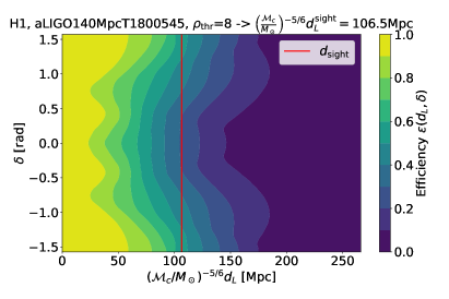
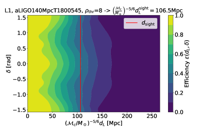
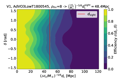
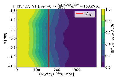
Figure 1: Efficiency, or average probability to detect a signal $\epsilon$, defined in Eq. (7), as a function of the normalized luminosity distance $d_{L}$ and the declination $\delta$ for the Hanford (H1), Livingston (L1) and Virgo (V1) interferometers, assuming O3-like sensitivities LIGO Scientific Collaboration et al. (2018); Buikema (2020); Acernese (2019). We also show the sight distance of each case, computed using Eqs. (20,21). For this plot and all other results in the paper, we assume the optimum SNR threshold of $\rho_{\mathrm{thr}}=8$.

In Fig. 1 we show the efficiency, or average probability to detect a signal $\epsilon$, defined in Eq. (7), as a function of the normalized luminosity distance $d_{L}$ and the declination $\delta$ for the Hanford (H1), Livingston (L1) and Virgo (V1) interferometers, assuming O3-like sensitivities LIGO Scientific Collaboration et al. (2018); Buikema (2020); Acernese (2019). We also show the joint sensitivity of the three interferometers at the same time. The efficiencies are simulated integrating Eq. (12) with Monte Carlo methods, uniformly sampling over time, polarization $\psi$ and $\cos\iota$. For this plot and all other results in the paper, we assume the optimum SNR threshold of $\rho_{\mathrm{thr}}=8$ Morras et al. (2023).

We observe that $\epsilon(d_{L},\delta)$ depends weakly on the declination $\delta$ because interferometers have a very broad angular sensitivity to GWs. The dependence with $\delta$ becomes even weaker when combining the interferometers, since they complement each other. Furthermore, we observe that $\epsilon$ monotonously decreases with distance to the source, since this will make the signals fainter and reduce the SNR. The way that $\epsilon(d_{L},\delta)$ decays with distance is determined by the sensitivity of the GW detectors involved. To quantify the sensitivity one usually uses the sight distance Maggiore (2007), which is computing by averaging $(\rho^{\mathrm{opt}}_{i})^{2}$ (Eq. (13)) over angles, and equating it to the SNR threashold. Using that $\langle|Q|^{2}\rangle=2/5$, we have:

$$d_{L,i}^{\mathrm{sight}}=\frac{1}{\rho_{\mathrm{thr}}}\frac{2}{5}\sqrt{\frac{5}{6}}\frac{c}{\pi^{2/3}}\left(\frac{G\mathcal{M}_{c}}{c^{3}}\right)^{5/6}\sqrt{\int_{f_{\mathrm{min}}}^{f_{\mathrm{max}}}{\rm d}f\frac{f^{-7/3}}{S_{i}(f)}}\,.$$ (20)

When we have multiple detectors, to be consistent with Eq. (19), we define the sight distance of the network as the result of adding the single detector sight distances in quadrature:

$$(d_{L,\mathrm{tot}}^{\mathrm{sight}})^{2}=\sum_{i}(d_{L,i}^{\mathrm{sight}})^{2}\,.$$ (21)

To see the dependance of the efficiency as a function of distance, we can define the declination averaged efficiency as

$$\bar{\epsilon}(d_{L})=\int_{-1}^{1}\frac{{\rm d}\sin{(\delta)}}{2}\,\epsilon(d_{L},\delta)\,.$$ (22)

In Fig. 2 we show this declination averaged efficiency $\bar{\epsilon}(d_{L})$ for the same cases as in Fig. 1. We observe that in all single interferometer cases, $\bar{\epsilon}(d_{L})$ behaves in the same way, having $100\%$ efficiency at $d_{L}=0$ and slowly loosing efficiency as the CBCs are placed further until we reach $0\%$ efficiency at $(5/2)d_{L}^{\mathrm{sight}}$. For the case of the three detector network, the shape of $\bar{\epsilon}(d_{L})$ is slightly different, having a bit of a sharper drop-off.

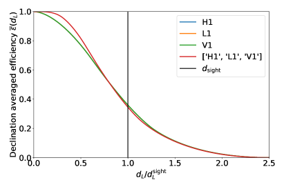
Figure 2: Declination averaged efficiency $\bar{\epsilon}(d_{L})$ as defined in Eq. (22) for the same cases as in Fig. 1. We normalize the luminosity distance by the sight distance of each case as defined in Eqs. (20, 21). Note that the lines for “H1”, “L1” and “V1” overlap, since the single detector declination averaged efficiencies are all the same.

III.2 Inhomogeneities in the local universe

For the purposes of showcasing the effects of the inhomogeneities in the measured rate of CBCs we will make the assumption that the rate is proportional to the matter density $\rho(\vec{x})$

$$R(\vec{x})\propto\rho(\vec{x})\,.$$ (23)

We do not expect this assumption to be true on very small scales, since the processes that generate binaries of compact objects which merge in the age of the universe will strongly depend on the properties of their local environment. However, in this section, we are going to explore merger rate inhomogeneities on large scales, of the order of megaparsecs (Mpc), over which we can assume that regions generating CBCs represent a similar fraction of matter, and therefore that the merger rate density is proportional to the matter density.

Furthermore, since we will be exploring small redshifts ($z\lesssim 0.08$), and to avoid confounding factors in showcasing the effects of the inhomogeneities, we will ignore the evolution of the merger rates with cosmic time, i.e. we assume that $\overline{R}(z)\approx\overline{R}_{0}$. Under these conditions, the event rate inhomogeneities will be equal to the matter over-density

$$\delta_{R}(\vec{x})=\delta_{M}(\vec{x})=\frac{\rho(\vec{x})-\overline{\rho}}{\overline{\rho}}\,.$$ (24)

These matter over-density have been well measured in the local universe using the peculiar (i.e. gravitational) velocities of galaxies Courtois et al. (2023) from the CosmicFlows (CF) catalogs Tully et al. (2016, 2023). In particular we take the $\delta_{M}(\vec{x})$ data published in Ref. Courtois et al. (2023), reconstructed from the grouped CF4, which reaches a redshift of $z=0.08$, i.e. a distance of $d\sim 340\mathrm{Mpc}/h_{70}$ having $64^{3}$ voxels. In Fig. 3 we show the distribution of the over-density $\delta_{M}$ in each of these voxels. We observe that while the distribution is peaked at $\delta_{M}=0$, being well approximated by a Gaussian in the $|\delta_{M}|\ll 1$ regime, it presents very large non Gaussian tails which are a direct consequence of the very non-linear structure present in our universe, formed by large voids ($\delta_{M}\sim-1$) and over-dense regions ($\delta_{M}\gtrsim 1$).

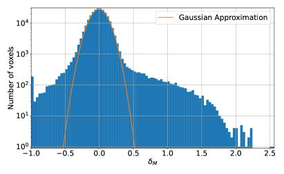
Figure 3: Histogram of the value of $\delta_{M}$ in the voxels of Ref. Courtois et al. (2023), reconstructed from the grouped CF4. The total number of voxels is $64^{3}=262144$. We also show a gaussian approximation, fitted in the range $\delta_{M}\in[-0.1,0.1]$.

To give a first estimate of how much these inhomogeneities will affect the merger rate density estimation, we temporarily assume that the probability to detect a signal does not depend on declination (i.e. $\epsilon(z,\delta)=\epsilon(z)$). Then, the $\langle VT\rangle$ could be computed as:

$$\langle VT\rangle=T\int_{0}^{z_{\mathrm{max}}}{\rm d}z\frac{dV_{c}}{dz}P(z)\epsilon(z)\frac{1}{1+z}\,,$$ (25)

where we have defined the angle averaged rate enhancement $P(z)$ as

$$P(z)=\frac{1}{4\pi}\int_{0}^{2\pi}{\rm d}\phi\int_{0}^{\pi}\sin{\theta}{\rm d}\theta\,(1+\delta_{M}(z,\theta,\phi))\,.$$ (26)

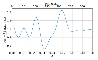
Figure 4: Angle averaged rate enhancement, as defined in Eq. (26) and computed using the $\delta_{M}(z,\theta,\phi)$ of Ref. Courtois et al. (2023).

In Fig. 4 we show this quantity as a function of redshift. We observe that deviations from 1 in the angle averaged rate enhancement $P(z)$ can be very large, of more than 20%. At large $z$ we expect $P(z)\to 1$, since we will be averaging the overdensities over a larger surface in the integral of Eq. (26). This is what is observed in Fig. 4. Note however, that there is a very large suppression at $z\sim 0.03$ ($d\sim 140~{}\mathrm{Mpc}/h_{70}$) followed by a large enhancement at $z\sim 0.05$ ($d\sim 210~{}\mathrm{Mpc}/h_{70}$), which are relatively large distances. These are caused by the Sloan Great Wall Gott et al. (2005), a huge structure in the local universe, which spans about $400~{}\mathrm{Mpc}/h_{70}$. The Sloan Great Wall is preceded by a correspondingly huge void, as can be seen in Fig. 4.

III.3 Effect of inhomogeneities in current GW detectors

In this section we will put together the results of Sec. III.1 and Sec. III.2 to give an estimate of the effect of inhomogeneities in current GW detectors.

Since we will consider our universe to be flat ($\Omega_{k}\sim 0$ Aghanim et al. (2020)) and the inhomogeneity data that we are using Courtois et al. (2023) contains redshifts $z\ll 1$, in Eq. (8) we have:

$$d_{c}(z)=d_{M}(z)\approx\frac{c}{H_{0}}z\left(1-\frac{3}{4}\Omega_{m}z+O(z^{2})\right)$$ (27)

where $\Omega_{m}=0.315\pm 0.007$ Aghanim et al. (2020), and the integral of Eq. (6) can be approximated as:

$$\langle VT\rangle\approx T\left(\frac{c}{H_{0}}\right)^{3}\int_{\Omega}{\rm d}\Omega\int_{0}^{z_{\mathrm{max}}}{\rm d}z\,z^{2}(1+\delta_{R}(\vec{x}))\epsilon(z,\delta)\times$$

$$\times\left[1-(3\Omega_{m}+1)z+O(z^{2})\right]\,.$$ (28)

For $z<0.08$, the value of the $O(z^{2})$ term we are ignoring is smaller that $1.5\%$.

To estimate the effect that inhomogeneities have on the $\langle VT\rangle$ of current GW detectors, we will use Eq. (28) to compute the ratio between the $\langle VT\rangle_{\mathrm{inhomo}}$, obtained setting $\delta_{R}$ to the matter inhomogeneities $\delta_{M}$ of Ref. Courtois et al. (2023), and $\langle VT\rangle_{\mathrm{homo}}$ assuming homogeneity (i.e. $\delta_{R}=0$). When computing the ratio $\langle VT\rangle_{\mathrm{inhomo}}/\langle VT\rangle_{\mathrm{homo}}$ we expect effects of the dependence of $\overline{R}(z)$ with cosmic time, wich is common in both cases, to largely cancel out.

The ratio $\langle VT\rangle_{\mathrm{inhomo}}/\langle VT\rangle_{\mathrm{homo}}$ is shown as a function of the sight distance for the different detectors in Fig. 5. We observe that this ratio has deviations of at most $6\%$ from unity, much smaller than the $O(20\%)$ deviations that were observed in the angle averaged rate enhancement $P(z)$ of Fig. 4. The reason the effect is suppressed is mainly because the efficiency is very extended in redshift (as can be seen in Fig. 2), averaging the effect of the inhomogeneities over different redshifts. The amplitude of the effect is very similar between interferometers, because as we saw in Fig. 1 the efficiency depends weakly on the inclination, however there are some small differences due to their different orientations with respect to the structure in the local universe.

Furthermore, looking at the top axes of Fig. 5 we can see that different sight distances will correspond to different CBC chirp masses (assuming O3-like sensitivities). As can be seen from Eq. (20), the more sensitive a detector is (smaller $S_{n}$), the larger the sight distance at a given mass. Even for O3-like sensitivities, the effects of the inhomogeneities on the $\langle VT\rangle$ estimation, which is relevant for $d_{L}\lesssim 140\mathrm{Mpc}$ will correspond to $\mathcal{M}_{c}\lesssim 1M_{\odot}$ in the single detector case and $\mathcal{M}_{c}\lesssim 0.5M_{\odot}$ in the case in which we consider the full H1-L1-V1 network. Therefore these results will be most relevant for the computation of the $\langle VT\rangle$ in searches of sub-solar mass (SSM) black holes Abbott et al. (2023c), which are used to put constraints on the merger rates of such objects and in turn to constrain models such as primordial black holes (PBH) Carr et al. (2024); Escrivà et al. (2022) and Dark Matter Black Holes Shandera et al. (2018).

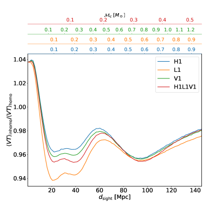
Figure 5: Ratio between $\langle VT\rangle\mathrm{s}$ computed using Eq. 28 setting $\delta_{R}(\vec{x})=\delta_{M}(\vec{x})$ from Ref. Courtois et al. (2023) ($\langle VT\rangle_{\mathrm{inhomo}}$) and setting $\delta_{R}(\vec{x})=0$ ($\langle VT\rangle_{\mathrm{homo}}$). The maximum sight distance shown of $d_{\mathrm{sight}}\sim 145~{}\mathrm{Mpc}=(2/5)d_{L}(z=0.08)$ is set to avoid the tails of the efficiencies (see Fig. 2) exiting the available data.

For Cosmic Explorer (CE) Evans et al. (2021) and Einstein Telescope (ET) Maggiore et al. (2020); Branchesi et al. (2023) we expect similar results to that of Fig. 5. However, due to the much higher sensitivities of these interferometers, we expect the luminosity distances to correspond to much smaller chirp masses, and therefore the effect will only be relevant for even smaller Black Holes. The durations of the signals from these tiny black holes inside the detector sensitivity band will be much longer and they would probably have to be looked for with continuous wave methods Miller et al. (2021); Alestas et al. (2024), instead of the matched filtering approach we have based our modeling of $\epsilon(z,\delta)$.

IV Conclusions

In this paper we have discussed the effect of inhomogeneities on the estimated merger rates of GW events, which can bias the measured local rate of GW events due to our particular location in the Universe. In Sec. II we show that the $\langle VT\rangle$, the quantity used to reconstruct the merger rates in GW data analysis, is given by the observation time $T$ multiplied by the integral over comoving volume of the population and time averaged efficiency $\epsilon(\vec{x})$, weighted by the normalized merger rate density $(1+\delta_{R}(\vec{x}))$.

We have then studied the effect of the inhomogeneous matter distribution of our local universe, obtained from CosmicFlows-4 Courtois et al. (2023), on the estimated rate of gravitational waves events in the LIGO/Virgo interferometers, assuming that the spatial distribution of events is proportional to the matter distribution. In Fig. 1 we observe that the effect of the angular inhomogeneities will be smoothed out by the low angular resolution of the interferometers, coupled with the rotation of the earth, which sweeps away any dependence of the average detection efficiency with the right ascension $\alpha$.

Furthermore, even though, as seen in Fig. 4, the redshift dependence of the local matter distribution has large variations (of the order of 20%) in the density contrast along the line of sight (averaged over spherical shells), the smooth dependence with redshift of the efficiency function (seen in Fig. 2), again averages out the inhomogeneities in redshift. In Fig. 5 we show that the local inhomogeneities give at most a 6% effect on the $\langle VT\rangle$ when compared with the homogeneous assumption, having a dependence with the sight distance, which will correspond with different chirp masses depending on the detector sensitivity. There is a trend; for distances below $\sim$10 Mpc, the ratio is always larger for the inhomogeneous distribution, while for distances from $\sim$10 to $\sim$200 Mpc it is always smaller. With sufficient statistics (i.e. hundreds of events in the nearby universe) we may be able to confirm whether GW events are correlated with the inhomogeneous matter distribution, as expected, or if they are uniformly distributed across the sky.

Extending the analysis to future detectors like the Einstein Telescope and Cosmic Explorer, with significantly better sensitivities, we can expect to be able to detect BBH mergers with smaller chirp masses at larger distances, and therefore be sensitive to the local matter inhomogeneities for smaller masses. One could then test the hypothesis of proportionality between BBH event rates and matter density. Moreover, for a large population of binary neutron star mergers, this may place a significant constraint on the local matter distribution Essick et al. (2023); Vitale et al. (2022).

Note that this analysis extends from the local group of galaxies to the cosmological homogeneity scale. However, for other type of events, like supernovae explosions Szczepanczyk et al. (2021) or close hyperbolic encounters García-Bellido and Nesseris (2017, 2018); Bini et al. (2024), the relevant inhomogeneities are those within our own galaxy. This requires a detailed 3D reconstruction of the Milky Way which may be possible in the near future with surveys like Gaia Prusti et al. (2016). We leave this analysis for a future work.

References

- Abbott et al. (2016a) B. P. Abbott et al. (LIGO Scientific, Virgo), Phys. Rev. Lett. 116, 061102 (2016a), arXiv:1602.03837 [gr-qc] .
- Aasi et al. (2015) J. Aasi et al. (LIGO Scientific), Class. Quant. Grav. 32, 074001 (2015), arXiv:1411.4547 [gr-qc] .
- Acernese et al. (2015) F. Acernese et al. (VIRGO), Class. Quant. Grav. 32, 024001 (2015), arXiv:1408.3978 [gr-qc] .
- Abbott et al. (2023a) R. Abbott et al. (KAGRA, VIRGO, LIGO Scientific), Phys. Rev. X 13, 041039 (2023a), arXiv:2111.03606 [gr-qc] .
- LIGO et al. (2023) LIGO, Virgo, and KAGRA, “O4 GraceDB public alerts,” (2023).
- Essick et al. (2023) R. Essick, W. M. Farr, M. Fishbach, D. E. Holz, and E. Katsavounidis, Phys. Rev. D 107, 043016 (2023), arXiv:2207.05792 [astro-ph.HE] .
- Vitale et al. (2022) S. Vitale, S. Biscoveanu, and C. Talbot, (2022), arXiv:2204.00968 [gr-qc] .
- Abbott et al. (2023b) R. Abbott et al. (KAGRA, VIRGO, LIGO Scientific), Phys. Rev. X 13, 011048 (2023b), arXiv:2111.03634 [astro-ph.HE] .
- Abbott et al. (2023c) R. Abbott et al. (LIGO Scientific, VIRGO, KAGRA), Mon. Not. Roy. Astron. Soc. 524, 5984 (2023c), [Erratum: Mon.Not.Roy.Astron.Soc. 526, 6234 (2023)], arXiv:2212.01477 [astro-ph.HE] .
- Courtois et al. (2023) H. M. Courtois, A. Dupuy, D. Guinet, G. Baulieu, F. Ruppin, and P. Brenas, Astron. Astrophys. 670, L15 (2023), arXiv:2211.16390 [astro-ph.CO] .
- Tully et al. (2014) R. B. Tully, H. Courtois, Y. Hoffman, and D. Pomarède, Nature 513, 71 (2014), arXiv:1409.0880 [astro-ph.CO] .
- Dupuy and Courtois (2023) A. Dupuy and H. M. Courtois, Astron. Astrophys. 678, A176 (2023), arXiv:2305.02339 [astro-ph.CO] .
- Dressler et al. (1987) A. Dressler, S. M. Faber, D. Burstein, R. L. Davies, D. Lynden-Bell, R. J. Terlevich, and G. Wegner, Astrophys. J. Lett. 313, L37 (1987).
- Gott et al. (2005) J. R. Gott, III, M. Juric, D. Schlegel, F. Hoyle, M. Vogeley, M. Tegmark, N. A. Bahcall, and J. Brinkmann, Astrophys. J. 624, 463 (2005), arXiv:astro-ph/0310571 .
- Alonso et al. (2015) D. Alonso, A. I. Salvador, F. J. Sánchez, M. Bilicki, J. García-Bellido, and E. Sánchez, Mon. Not. Roy. Astron. Soc. 449, 670 (2015), arXiv:1412.5151 [astro-ph.CO] .
- Tully et al. (2016) R. B. Tully, H. M. Courtois, and J. G. Sorce, Astron. J. 152, 50 (2016), arXiv:1605.01765 [astro-ph.CO] .
- Tully et al. (2023) R. B. Tully et al., Astrophys. J. 944, 94 (2023), arXiv:2209.11238 [astro-ph.CO] .
- Biswas et al. (2009) R. Biswas, P. R. Brady, J. D. E. Creighton, and S. Fairhurst, Class. Quant. Grav. 26, 175009 (2009), [Erratum: Class.Quant.Grav. 30, 079502 (2013)], arXiv:0710.0465 [gr-qc] .
- Abbott et al. (2016b) B. P. Abbott et al. (LIGO Scientific, Virgo), Astrophys. J. Lett. 833, L1 (2016b), arXiv:1602.03842 [astro-ph.HE] .
- Tiwari (2018) V. Tiwari, Class. Quant. Grav. 35, 145009 (2018), arXiv:1712.00482 [astro-ph.HE] .
- Chen et al. (2017) H.-Y. Chen, R. Essick, S. Vitale, D. E. Holz, and E. Katsavounidis, Astrophys. J. 835, 31 (2017), arXiv:1608.00164 [astro-ph.HE] .
- Chu et al. (2022) Q. Chu et al., Phys. Rev. D 105, 024023 (2022), arXiv:2011.06787 [gr-qc] .
- Usman et al. (2016) S. A. Usman et al., Class. Quant. Grav. 33, 215004 (2016), arXiv:1508.02357 [gr-qc] .
- Sachdev et al. (2019) S. Sachdev et al., (2019), arXiv:1901.08580 [gr-qc] .
- Aubin et al. (2021) F. Aubin et al., Class. Quant. Grav. 38, 095004 (2021), arXiv:2012.11512 [gr-qc] .
- Maggiore (2007) M. Maggiore, Gravitational Waves. Vol. 1: Theory and Experiments, Oxford Master Series in Physics (Oxford University Press, 2007) p. 572.
- Jaranowski et al. (1998) P. Jaranowski, A. Krolak, and B. F. Schutz, Phys. Rev. D 58, 063001 (1998), arXiv:gr-qc/9804014 .
- LIGO Scientific Collaboration et al. (2018) LIGO Scientific Collaboration, Virgo Collaboration, and KAGRA Collaboration, “LVK Algorithm Library - LALSuite,” Free software (GPL) (2018).
- Buikema (2020) A. e. a. Buikema, Phys. Rev. D 102, 062003 (2020).
- Acernese (2019) F. e. a. Acernese (Virgo Collaboration), Phys. Rev. Lett. 123, 231108 (2019).
- Morras et al. (2023) G. Morras, J. F. N. n. Siles, J. Garcia-Bellido, and E. R. Morales, Phys. Rev. D 107, 023027 (2023), arXiv:2209.05475 [gr-qc] .
- Aghanim et al. (2020) N. Aghanim et al. (Planck), Astron. Astrophys. 641, A6 (2020), [Erratum: Astron.Astrophys. 652, C4 (2021)], arXiv:1807.06209 [astro-ph.CO] .
- Carr et al. (2024) B. Carr, S. Clesse, J. Garcia-Bellido, M. Hawkins, and F. Kuhnel, Phys. Rept. 1054, 1 (2024), arXiv:2306.03903 [astro-ph.CO] .
- Escrivà et al. (2022) A. Escrivà, F. Kuhnel, and Y. Tada, (2022), arXiv:2211.05767 [astro-ph.CO] .
- Shandera et al. (2018) S. Shandera, D. Jeong, and H. S. G. Gebhardt, Phys. Rev. Lett. 120, 241102 (2018), arXiv:1802.08206 [astro-ph.CO] .
- Evans et al. (2021) M. Evans et al., (2021), arXiv:2109.09882 [astro-ph.IM] .
- Maggiore et al. (2020) M. Maggiore, C. V. D. Broeck, N. Bartolo, E. Belgacem, D. Bertacca, M. A. Bizouard, M. Branchesi, S. Clesse, S. Foffa, J. García-Bellido, S. Grimm, J. Harms, T. Hinderer, S. Matarrese, C. Palomba, M. Peloso, A. Ricciardone, and M. Sakellariadou, Journal of Cosmology and Astroparticle Physics 2020, 050 (2020).
- Branchesi et al. (2023) M. Branchesi et al., JCAP 07, 068 (2023), arXiv:2303.15923 [gr-qc] .
- Miller et al. (2021) A. L. Miller, S. Clesse, F. De Lillo, G. Bruno, A. Depasse, and A. Tanasijczuk, Phys. Dark Univ. 32, 100836 (2021), arXiv:2012.12983 [astro-ph.HE] .
- Alestas et al. (2024) G. Alestas, G. Morras, T. S. Yamamoto, J. García-Bellido, S. Kuroyanagi, and S. Nesseris, (2024), arXiv:2401.02314 [astro-ph.CO] .
- Szczepanczyk et al. (2021) M. Szczepanczyk et al., Phys. Rev. D 104, 102002 (2021), arXiv:2104.06462 [astro-ph.HE] .
- García-Bellido and Nesseris (2017) J. García-Bellido and S. Nesseris, Phys. Dark Univ. 18, 123 (2017), arXiv:1706.02111 [astro-ph.CO] .
- García-Bellido and Nesseris (2018) J. García-Bellido and S. Nesseris, Phys. Dark Univ. 21, 61 (2018), arXiv:1711.09702 [astro-ph.HE] .
- Bini et al. (2024) S. Bini, S. Tiwari, Y. Xu, L. Smith, M. Ebersold, G. Principe, M. Haney, P. Jetzer, and G. A. Prodi, Phys. Rev. D 109, 042009 (2024), arXiv:2311.06630 [gr-qc] .
- Prusti et al. (2016) T. Prusti et al., Astronomy & Astrophysics 595, A1 (2016).