Optimal Transmission Power Scheduling for Networked Control System under DoS Attack
Abstract
Designing networked control systems that are reliable and resilient against adversarial threats, is essential for ensuring the security of cyber-physical systems. This paper addresses the communication-control co-design problem for networked control systems under denial-of-service (DoS) attacks. In the wireless channel, a transmission power scheduler periodically determines the power level for sensory data transmission. Yet DoS attacks render data packets unavailable by disrupting the communication channel. This paper co-designs the control and power scheduling laws in the presence of DoS attacks and aims to minimize the sum of regulation control performance and transmission power consumption. Both finite- and infinite-horizon discounted cost criteria are addressed, respectively. By delving into the information structure between the controller and the power scheduler under attack, the original co-design problem is divided into two subproblems that can be solved individually without compromising optimality. The optimal control is shown to be certainty equivalent, and the optimal transmission power scheduling is solved using a dynamic programming approach. Moreover, in the infinite-horizon scenario, we analyze the performance of the designed scheduling policy and develop an upper bound of the total costs. Finally, a numerical example is provided to demonstrate the theoretical results.
Index Terms:
SINR-based communication model, transmission power schedule, DoS attack, infinite-horizon discounted costI Introduction
Cyber-physical systems are systems that integrate sensors, controllers, and actuators to collaborate over a communication network for regulating and optimizing the behavior of a dynamic system [1, 2]. There are many applications such as robotics [3], smart grids [4], and intelligent vehicle [5]. These networked systems generally assume that data are measured and transmitted periodically to update control signals [6]. However, transmitting sensory data over a communication network is costly in general due to limited battery energy and communication channel bandwidth. This fact motivates us to co-design the control and communication strategies to ensure that the valuable sensory data is efficiently transmitted to the controller, thereby improving overall system performance.
Due to increased connectivity, these cyber-physical systems are suffering from cyber threats. Two most common cyber attacks are deception attacks and denial-of-service (DoS) attacks [7]. Deception attacks degenerate the system performance by maliciously modifying the information contained in transmitted data [8, 9, 10]. DoS attacks render data packets unavailable by jamming communication channels [11, 12]. It is more destructive compared to deception attacks when facing threats from large-scale and persistent attacks. Considering the detrimental impact of cyberattacks on control performance, proactive risk management strategies are essential to ensure the resilience of networked control systems.
Transmission power scheduling means that the transmission device dynamically adjusts power levels according to the changing network conditions to fulfill requirements of cyber-physical systems [13, 14]. Compared to the traditional event-based triggering, power scheduling allows for continuous optimization of energy usage, which is crucial for battery-powered devices and energy-constrained environments. Increasing transmission power levels typically enhances communication link reliability. As a consequence, the power scheduler envisions a tradeoff between energy usage and improved control performance by reliable transmission. To address this issue, the authors in [14] investigate the optimal power scheduling in remote estimation. Moreover, [13, 15] investigate the co-design of power scheduling and control strategies for networked control. However, none of the above works take cyber attacks into consideration. Some works, e.g., [16, 17], investigate the power allocation under the DoS attack to minimize the long-term mean square error covariance and propose a variance-based scheduling mechanism. However, variance-based scheduling does not utilize real-time innovations when making decisions and thus is generally outperformed by state-based scheduling [18]. In real-world applications such as financial investment, current rewards are typically valued more than future rewards. Thus, this article aims to obtain a co-design strategy that minimizes the expectation of a discounted accumulated cost.
In this work, we propose a framework to jointly co-design the control law and power scheduler for the networked control system under DoS attack. We consider a signal-to-interference-plus-noise ratio (SINR)-based network model [17], where the transmission success probability is affected by the transmission power level chosen by the scheduler and the energy imposed by the attacker. The contribution of this work is summarized as follows. For both cases, the optimal co-design of control and scheduling is shown to be separable, given that the knowledge about the attack energy is symmetric between the controller and the scheduler. The optimal control law is shown to be certainty equivalent. By applying the dynamic programming approach to the remaining sequential decision problem, the condition for optimal power scheduling is derived. Further, in the infinite-horizon case, we provide an upper bound on the total cost achieved by the designed power scheduler.
The remainder of this article is structured as follows: Section II introduces preliminaries. Section III and Section IV present the main result on optimal co-design of control and transmission power scheduling in finite-horizon and infinite-horizon cases, respectively. Section V presents numerical simulations. Section VI concludes this work.
Notations. Denote by and the set of real numbers and the set of the -tuples of real numbers, respectively. Denote by the set of nonnegative integers. For and , the set denotes . Denote as the history of state during time . For a random variable , implies that is distributed according to the distribution . Denote , and as the expectation, the conditional expectation and the covariance of the random variable, respectively. If the random variable follows a normal distribution with the mean of and the covariance of , we write . Denote by the probability density function of a -dimension random vector . Denote by the tail function of the standard Gaussian distribution. Denote the spectral radius of as .
II Preliminaries
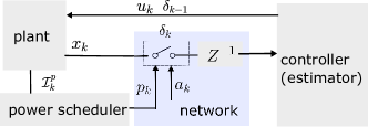
We consider the energy-constrained feedback control system over the communication network, as illustrated in Fig. 1. The scheduler periodically determines the power of transmitting sensory data, which affects packets’ transmission success probability. The controller generates the control signal based on the remote estimate.
II-A System model
The discrete-time stochastic dynamical system to be controlled is described as
| (1) |
where and are the state vector and the control force, respectively. The system matrices are given by , , where the pair is controllable. The process noise is assumed to be independent identically distributed (i.i.d.) Gaussian processes with zero mean and positive semi-definite variance . The initial state is a random vector that is statistically independent of for all .
II-B Network model
The sensor located at the plant side periodically accesses the system states, as in Fig. 1. The power-constrained scheduler determines the power used to send out packets at time , where and denote the power scheduling law and the locally available information set of the power scheduler, respectively. Moreover, denote as the admissible transmission power set with being the maximum transmission power.
Consider an additive white Gaussian noise (AWGN) channel using quadrature amplitude modulation [17]. In the presence of a DoS interference attacker, the communication channel is modeled as , where is the additive white Gaussian noise power, and is the interference power from the attacker [19]. The following assumptions are for the attack energy.
Assumption 1
-
1.
The attack energy , for , is a i.i.d. random process with a continuous distribution .
-
2.
The attack energy with and being a positive scalar.
-
3.
The random variable , , is independent of process noise , for all , and the initial state .
The attack energy can be interpreted as a channel fading parameter that encompasses unpredictable variations in the wireless channel [13]. The subsequent sections will discuss control and power scheduling co-design, considering known and unknown attack energy scenarios, respectively.
Denote the transmission success as a random binary process , where denotes the packet is transmitted successfully, and otherwise. The packet dropout probability is affected by the transmission power and attack energy:
| (2) |
where is a communication channel parameter and is the tail function of the standard Gaussian distribution. Moreover, . Note that a higher transmission power indicates a lower packet dropout probability and vice versa. Assume that the network induces a one-step delay. At time , the packet arrives at the remote side is if , and otherwise, with . The remote estimator is given as
| (3) |
with the initial value , and denotes the remote information set. The control signal is generated according to control law , where with being the admissible control law set. Then, the remote information set available for the controller is defined as with the initial value . Moreover, assume that the transmission success index will be returned to the local side with a one-step delay. Thus, the local information set available for the power scheduler by time is with the initial value .
This article aims to co-design the power scheduler and control law to optimize control performance with limited transmission energy. More specifically, we consider both finite- and infinite-horizon problems.
Problem 1
(Finite-horizon problem) Find the optimal power scheduler and the control law by solving the following finite-horizon optimization problem:
| (4) |
where the scalar denotes the tradeoff multiplier. The control performance is defined as
| (5) |
where is the discount factor. The matrices , are semi-definite positive and is definite positive, respectively. Assume that the pair is detectable, with . Moreover, the total transmission energy consumption is measured by .
Problem 2
(Infinite-horizon problem) Find the optimal power scheduler and the control law by solving the following infinite-horizon optimization problem:
| (6) |
with being the infinite-horizon LQG function:
| (7) |
where , and the transmission energy consumption is .
The discount factor reflects how immediate and future costs are weighted. A higher discount factor places more weight on future costs and vice versa.
III Finite-horizon case
In this section, we develop the solution to Problem 1. In the following, we will decompose the co-design optimization problem and design the optimal control law.
III-A Optimal control
In networked control systems, the controller may induce a dual effect: 1) stabilizing the dynamic system and 2) probing the system to reduce uncertainties. This leads to a nonclassical information structure between the power scheduler and the controller. In other words, the information available to two distributed decision makers might be asymmetric. We provide the following notion to facilitate the search for the structural results of the optimization problem.
Definition 1
(Dominating policy) Denote as the set of all admissible policy pairs . Consider the cost function defined in the corresponding problem. A set of policy pairs is called a dominating class of policies, if for any feasible , there exists a feasible , such that .
The following lemma decomposes the original co-design optimization problem, assuming that the attack energy is known, and investigates which class of policies is dominating for problem (4).
Lemma 1
Consider an admissible scheduling policy set , in which function only depends on random variables . Then the set is a dominating class of policies, where is the certainty equivalence controller:
| (8) |
with , and is solved from algebraic Riccati equation [20]:
| (9) | |||||
with .
Proof. Assume that there exists a triggering law being the function of random variables . Note that the information pattern of the power scheduler and the controller are nested, i.e., . In addition, we can see that can be fully recovered from and , which is inferred from accessible to the local scheduler. Therefore, there exists a policy pair producing identical decision variables as almost surely, i.e., holds almost surely. In other words, there exists a policy pair that achieves the same cost as . Denote the remote estimation error as . According to (3), we have . Under the control law that is symmetric with respect to innovation , we have , see [21]. Then the remote estimation error evolves as
| (10) |
with the initial value . Note that comprises primitive random variables and . Substituting the algebraic Riccati equation into the cost function (4), we have
| (11) | |||||
with . Note that the first, the second, and the last terms of (11) are independent of the control policy . Substituting with , we have
| (12) | |||||
where the second equality is from the tower property of conditional expectation, i.e., and . Then the optimal controller minimizing (11) results in (8). Moreover, we have , where depends on , and the first and the last equalities follow from . Namely, for any feasible , the set is a dominating class of policy pairs such that .
Lemma 1 implies that the original co-design problem can be decomposed into two subproblems, i.e., optimal power scheduling design that depends on primitive random variables and the optimal control law design, without loss of optimality.
III-B Optimal power scheduling
The following theorem will develop the optimal power scheduler in the finite horizon scenario.
Theorem 1
Proof. Substituting the optimal controller (8) into (11) yields
| (17) | |||||
Taking the conditional expectation of with respect to , and by (10), we have
| (18) | |||||
where the second equality establishes as and is independent of , the last equality follows from . Then the original optimization problem (4) is reduced to
| (19) |
We omit the remaining terms of (17) and the last term of (18) as they are independent of . Note that can be fully recovered by the local power scheduler as . Let us apply the dynamic programming approach to (19). Synthesizing the optimal scheduler boils down to characterize the value function , which is defined as in (15). Moreover, we have
| (20) |
which follows from the law of total expectation. Substituting (III-B) into (15) yields (13), which gives the optimal power scheduler in (16).
Remark 1
Theorem 1 characterizes the optimal power scheduler for the finite-horizon problem (4). Note that it is difficult to compute in (13), in particular for a long horizon . Alternatively, there is a practical greedy way to approximate as follows
| (21) |
with defined in (14). The greedy scheduling policy solved from (21) is suboptimal yet has a rather low computation complexity.
Theorem 1 assumes that the attack energy is known, the following proposition considers the case when attack energy is unknown.
Proposition 1
Consider the optimization problem (4) for system (1).
If the attack energy is unknown, consider an admissible scheduling policy set , which only depends on random variables .
Then the set with given by (8) is a dominating class of policies.
Proof.
Note that removing the attack energy from the information sets and does not alter the information structure between the local power scheduler and the remote controller.
It follows the proof of Lemma 1.
Then the set constituted by a power scheduling and the certainty equivalence controller (8) is a class of dominating policies.
Next, we provide an approximation to the optimal scheduler when the attack energy is unknown. It follows from the proof of Theorem 1. Then, we consider the optimisation problem (19). Taking the expectation of over the distribution yields
| (22) |
Then we replace with in scheduling policy (13) and (14). Then, an approximation-based greedy scheduling is
| (23) |
IV Infinite-horizon case
In this section, we consider the infinite-horizon problem, i.e., Problem 2. Since the pair is controllable, the algebraic Riccati equation
| (24) |
has a unique and positive semi-definite solution . Accordingly, matrices , are written as , and . The following assumption is essential for characterizing the optimal stationary scheduler.
Assumption 2
The minimum achievable packet dropout probability under the attack energy , i.e., satisfies
Lemma 2
The set is a dominating class of policies, where is given by the certainty equivalence controller:
| (25) |
with .
Proof. It follows from the proof of Lemma 1.
Next we consider how to synthesize the optimal power scheduler. From (17), the cost function under the optimal control policy (25) is rewritten as
| (26) |
Accordingly, the optimization problem (6) is reduced to
| (27) |
with the per-stage cost defined in (14), and initial value . We next formulate the optimization problem (27) as a MDP with the control model , where denotes the state space, denotes the action space, denotes the Borel measurable transition kernel defined on . Note that obeys a distribution of . Denote as the next states of and , respectively. Denote as the transition probability from to . By (10), we have
| (28) | |||||
where is the probability density function of the random variable . Note that (28) holds as the process noise is independent of attack energy and is the current decision.
According to the optimization problem (27), define an associated -stage cost under the policy :
| (29) |
with the initial value and . The decision variables for is chosen according to policy . Let be a class of nonnegative and lower semi-continuous (l.s.c.) functions on . Define the value iteration sequence , for and :
| (30) | |||||
where denotes a non-empty set associated to , for any . Then, we have given initial value , for .
The following proposition shows that there exists an optimal stationary policy for the optimization problem (27).
Proposition 2
Proof. According to [22], we need to verify the following conditions:
-
1.
is nonnegative, l.s.c. and inf-compact on ;
-
2.
the transition law is weakly continuous;
-
3.
the multifunction is l.s.c.;
-
4.
there exists a policy such that for each .
The first condition holds by the definition of , as in (14). It is inf-compact on as the set is compact. The second condition holds as is continuous on . Then for any continuous and bounded function on , the map is continuous on . The third condition holds as is convex, see [23].
To verify the last condition, we choose for all . Then, . The expected dropout probability under is
| (32) |
The next is to calculate . Denote . By the expression of estimation error as in (10), we have
| (36) |
Accordingly, define , When , . When ,
When ,
By induction, for all , we have
| (37) | |||||
Sum (37) over all , we obtain
| (38) |
Note that when , . Then Assumption 2 is sufficient for its establishment. Moreover, we have
| (39) | |||||
The total transmission cost under power scheduling law is written as
| (40) |
Combine (IV), (39) and (40), we obtain that
Conditions 1-4) are verified. According to [22], claims 1-3) holds.
The following theorem develops the optimal scheduler and the cost achieved by the designed scheduling policy.
Theorem 2
Consider the optimization problem (6) for system (1). Fix the optimal control law as the certainty equivalence controller (25). Let Assumption 2 hold and let
| (41) |
where is solved from (31).
-
1.
The optimal power scheduler is given by
(42) -
2.
Let be the solution of Laypunov equation:
(43) where is given by (32). The total cost achieved by the optimal power scheduler and the optimal control is upper-bounded by
(44)
V Simulation
In this section, we provide numerical examples to illustrate our results. Consider a second-order system with system dynamics , , process noise covariance . The weighting matrices in the LQG function (5) are chosen as . The discount factor is chosen as . The covariance of the initial value is chosen as .
The communication channel parameters are chosen as , , see [17]. The attack energy is chosen as a uniformly distributed random variable between .
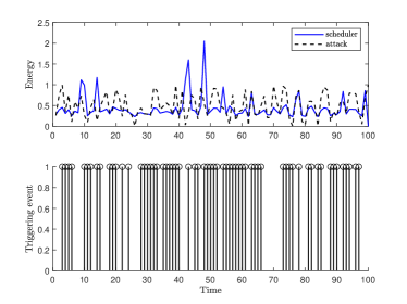
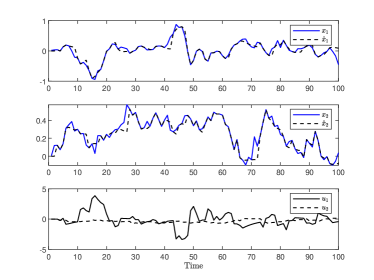
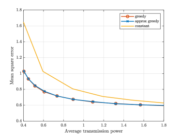
We choose the time horizon as and the tradeoff multiplier as . The top subfigure of Fig. 2 depicts the energy of the attack and the transmission power determined by scheduler (21) during . The button subfigure of Fig. 2 depicts the transmission success index during . It can be observed from Fig. 3 that transmission success is affected by both the transmission power and attack energy. When addressing the resource utilization efficiency under attacks, a higher attack energy generally leads a higher transmission power. Fig. 3 depicts the system state trajectory, its estimate, and control signal. It can be observed from Fig. 3 that the remote estimator effectively tracks the system dynamics. Fig. 4 depicts the mean square error under different average transmission power achieved by the greedy schedulers (21) and (22) and the scheduler with constant transmission power for . The mean square error is measured by and the average transmission power is measured by . It can be observed that using the same average transmission power, greedy schedulers (21) and (22) achieves smaller mean square error than constant-power schedulers.
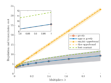
Fig. 5 depicts the total regulation and transmission costs under different multipliers under the greedy scheduler (21), the approximation-based greedy scheduler (22) assuming attack energy is unknown, and constant-power schedulers. We choose tradeoff multiples . Monte Carlo simulation runs trials. As in (17), only last-second terms depend on the designed control and scheduling laws. We choose as the empirical total regulation and transmission cost. For the empirical results, shaded areas represent one standard deviation over 20000 trials. Accordingly, the theoretical upper bound of the total cost, i.e., the cost achieved by a transmission scheduler with maximum constant power, is . The empirical upper bound is calculated by implementing the constant-power scheduler for all . It can be observed from Fig. 5 that the theoretical upper bound of the total cost approaches the empirical one. As a comparison, we also depict the lower bound of the total cost by a constant-power scheduler, i.e., the best performance it can achieve, which is given by
Moreover, it can be observed that greedy schedulers (21) and (22) both outperform the schedulers with constant power, which includes the one that achieves the minimum cost among all constant-power schedulers.
VI Conclusion
In this article, we have studied the optimal co-design of control law and transmission power scheduler that minimizes the regulation and transmission costs for networked control systems under DoS attacks. Given the acknowledgment signal from the remote controller, the information structure between the controller and the power scheduler is nested. Therefore, we showed that the original co-design can be decomposed into the optimal control design, yielding a certainty equivalence controller, and the optimal power scheduling design, which is tracked by dynamic programming approaches. Expressions of the optimal power scheduling were provided in both finite- and infinite-horizon cases. To ease the computational complexity in finite-horizon dynamic programming, an alternative greedy scheduler was developed for implementation. Additionally, in the infinite-horizon case, we provided the upper bound of the total regulation and transmission cost under the proposed scheduler.
References
- [1] W. Zhang, M. S. Branicky, and S. M. Phillips, “Stability of networked control systems,” IEEE control systems magazine, vol. 21, no. 1, pp. 84–99, 2001.
- [2] Y. Jiang, S. Wu, R. Ma, M. Liu, H. Luo, and O. Kaynak, “Monitoring and defense of industrial cyber-physical systems under typical attacks: From a systems and control perspective,” IEEE Transactions on Industrial Cyber-Physical Systems, 2023.
- [3] Z. Yan, N. Jouandeau, and A. A. Cherif, “A survey and analysis of multi-robot coordination,” International Journal of Advanced Robotic Systems, vol. 10, no. 12, p. 399, 2013.
- [4] A. K. Singh, R. Singh, and B. C. Pal, “Stability analysis of networked control in smart grids,” IEEE Transactions on Smart Grid, vol. 6, no. 1, pp. 381–390, 2014.
- [5] S. E. Li, Y. Zheng, K. Li, L.-Y. Wang, and H. Zhang, “Platoon control of connected vehicles from a networked control perspective: Literature review, component modeling, and controller synthesis,” IEEE Transactions on Vehicular Technology, 2017.
- [6] A. Molin and S. Hirche, “Suboptimal event-triggered control for networked control systems,” ZAMM - Journal of Applied Mathematics and Mechanics, vol. 94, no. 4, pp. 277–289, 2014.
- [7] S. Amin, A. A. Cárdenas, and S. S. Sastry, “Safe and secure networked control systems under denial-of-service attacks,” in Hybrid Systems: Computation and Control: 12th International Conference, HSCC 2009, San Francisco, CA, USA, April 13-15, 2009. Proceedings 12, pp. 31–45, Springer, 2009.
- [8] A. Teixeira, D. Pérez, H. Sandberg, and K. H. Johansson, “Attack models and scenarios for networked control systems,” in Proceedings of the 1st international conference on High Confidence Networked Systems, pp. 55–64, 2012.
- [9] H. Zhu, L. Xu, Z. Bao, Y. Liu, L. Yin, W. Yao, C. Wu, and L. Wu, “Secure control against multiplicative and additive false data injection attacks,” IEEE Transactions on Industrial Cyber-Physical Systems, 2023.
- [10] L. Xu, H. Zhu, K. Guo, Y. Gao, and C. Wu, “Output-based secure control under false data injection attacks,” IEEE Transactions on Industrial Cyber-Physical Systems, 2024.
- [11] Y. Dai, M. Li, K. Zhang, and Y. Shi, “Robust and resilient distributed mpc for cyber-physical systems against dos attacks,” IEEE Transactions on Industrial Cyber-Physical Systems, 2023.
- [12] S. Feng, A. Cetinkaya, H. Ishii, P. Tesi, and C. De Persis, “Networked control under dos attacks: Tradeoffs between resilience and data rate,” IEEE Transactions on Automatic Control, vol. 66, no. 1, pp. 460–467, 2020.
- [13] K. Gatsis, A. Ribeiro, and G. J. Pappas, “Optimal power management in wireless control systems,” IEEE Transactions on Automatic Control, vol. 59, no. 6, pp. 1495–1510, 2014.
- [14] X. Ren, J. Wu, K. H. Johansson, G. Shi, and L. Shi, “Infinite horizon optimal transmission power control for remote state estimation over fading channels,” IEEE Transactions on Automatic Control, vol. 63, no. 1, pp. 85–100, 2017.
- [15] T. Soleymani, J. S. Baras, S. Hirche, and K. H. Johansson, “Feedback control over noisy channels: Characterization of a general equilibrium,” IEEE Transactions on Automatic Control, 2021.
- [16] Y. Li, L. Shi, P. Cheng, J. Chen, and D. E. Quevedo, “Jamming attacks on remote state estimation in cyber-physical systems: A game-theoretic approach,” IEEE Transactions on Automatic Control, vol. 60, no. 10, pp. 2831–2836, 2015.
- [17] Y. Li, D. E. Quevedo, S. Dey, and L. Shi, “Sinr-based dos attack on remote state estimation: A game-theoretic approach,” IEEE Transactions on Control of Network Systems, vol. 4, no. 3, pp. 632–642, 2016.
- [18] J. Wu, Y. Yuan, H. Zhang, and L. Shi, “How can online schedules improve communication and estimation tradeoff?,” IEEE Transactions on Signal Processing, vol. 61, no. 7, pp. 1625–1631, 2013.
- [19] J. G. Proakis, Digital communications. McGraw-Hill, Higher Education, 2008.
- [20] K. J. Ȧström, Introduction to stochastic control theory. Dover Publications, 2006.
- [21] T. Soleymani, J. S. Baras, S. Hirche, and K. H. Johansson, “Value of information in feedback control: Global optimality,” IEEE Transactions on Automatic Control, 2022.
- [22] O. Hernández-Lerma and M. Muñoz de Ozak, “Discrete-time markov control processes with discounted unbounded costs: optimality criteria,” Kybernetika, vol. 28, no. 3, pp. 191–212, 1992.
- [23] O. Hernández-Lerma and W. J. Runggaldier, “Monotone approximations for convex stochastic control problems,” Journal of Mathematical Systems, Estimation, and Control, vol. 4, no. 4, pp. 99–140, 1994.