Causal Contrastive Learning
for Counterfactual Regression Over Time

Abstract

Estimating treatment effects over time holds significance in various domains, including precision medicine, epidemiology, economy, and marketing. This paper introduces a unique approach to counterfactual regression over time, emphasizing long-term predictions. Distinguishing itself from existing models like Causal Transformer, our approach highlights the efficacy of employing RNNs for long-term forecasting, complemented by Contrastive Predictive Coding (CPC) and Information Maximization (InfoMax). Emphasizing efficiency, we avoid the need for computationally expensive transformers. Leveraging CPC, our method captures long-term dependencies in the presence of time-varying confounders. Notably, recent models have disregarded the importance of invertible representation, compromising identification assumptions. To remedy this, we employ the InfoMax principle, maximizing a lower bound of mutual information between sequence data and its representation. Our method achieves state-of-the-art counterfactual estimation results using both synthetic and real-world data, marking the pioneering incorporation of Contrastive Predictive Encoding in causal inference.

1 Introduction

It’s vital in real-world applications to estimate potential responses, i.e., responses under hypothetical treatment strategies. Individuals show diverse responses to the same treatment, emphasizing the need to quantify individual response trajectories. This enables personalized interventions, enhancing decision-making efficacy. In medical contexts, precise response estimation enables tailored treatments for patients [Atan et al., 2018, Shalit, 2020, Mueller and Pearl, 2023].

This paper focuses on counterfactual regression over time, estimating responses under hypothetical treatment plans based on individual records, including past covariates, responses, and treatment sequences up to the current prediction time [Robins et al., 2000, Robins and Hernán, 2009a]. In addressing the challenges of this time-varying setting, we tackle: (1) Time-dependent confounding [Platt et al., 2009]: confounders influenced by past treatment, impacting subsequent treatments and responses. (2) Selection bias:imbalanced covariate distributions across treatment regimes in observational data, requiring time-aware handling beyond methods in static settings [Robins et al., 2000, Schisterman et al., 2009, Lim, 2018a]. (3) Long-term dependencies: enduring interdependencies among covariates, treatments, and responses, enabling long-range interactions [Choi et al., 2016, Pham et al., 2017].

Recent neural network advancements, like Recurrent Marginal Structural Networks (RMSNs) [Lim, 2018b], Counterfactual Recurrent Networks (CRN) [Bica et al., 2020a], and G-Net Li et al. [2021], attempted to address these causal inference challenges. However, given the limitations of these models, particularly in capturing long-term dependencies due to their sole reliance on RNNs networks, recent studies Melnychuk et al. [2022] suggest integrating transformers to improve temporal dynamics representation. Instead of viewing this as a drawback for RNNs, we consider it an opportunity to emphasize their strengths. We craft architectures tailored for counterfactual regression over large horizons without resorting to complex, challenging-to-interpret models like transformers. Our approach leverages the computational efficiency of RNNs while incorporating Contrastive Predictive Coding (CPC) Oord et al. [2018], Henaff [2020] for data history representation learning. This strategic use of RNNs not only enhances model performance but also contributes to efficiency, providing a compelling alternative to transformer-based approaches.

Furthermore, we usually formulate identification assumptions of counterfactual responses over the original process history space (Appendix B.1). However, these assumptions may not hold over the representation space for an arbitrary representation function. As identification assumptions often involve conditional independence, they apply when using an invertible representation function. Current models for time-varying settings [Lim, 2018b, Bica et al., 2020a, Melnychuk et al., 2022] do not explicitly or implicitly enforce representation invertibility. To address this, instead of adding complexity with a decoder, we implicitly push the history process to be "reconstructable" from the encoded representation by maximizing Mutual Information (MI) between representation and input. This approach originates from the InfoMax principle Linsker [1988] and is akin to Deep InfoMax Hjelm et al. [2019].

2 Contributions

Our approach is inspired by self-supervised learning utilizing MI objectives Hjelm et al. [2019]. We aim to maximize MI between different views of the same input, introducing counterfactual regression over time by incorporating CPC to learn long-term dependencies. Additionally, we propose a tractable lower bound to the original InfoMax objectives for more efficient representations. This is challenging due to the sequential nature and high dimensionality, constituting a novelty. We demonstrate the importance of both regularization terms through an ablation study. Previous work leveraging contrastive learning for causal inference applies only to the static setting with no theoretical grounding Chu et al. [2022]. To our knowledge, we frame for the first time the representation balancing problem from an information-theoretic perspective and show that the suggested adversarial game (Theorem 5.4) yields theoretically balanced representations using the Contrastive Log-ratio Upper Bound (CLUB) of MI, computed efficiently. Our novel model, termed Causal CPC, introduces several key innovations: (1) We showcase the capability of leveraging CPC to capture long-term dependencies within the process history using InfoNCE [Gutmann and Hyvärinen, 2010, 2012, Oord et al., 2018], which is an unexplored area in counterfactual regression over time and its integration to model the process history is not straightforward in causality. (2) We enforce input reconstruction from representation by contrasting the representation with its input. Such quality is generally overlooked in baselines, yet it ensures that confounding information is retained, preventing biased counterfactual estimation. (3) Applying InfoMax to process history while respecting its dynamic nature is challenging. We provide a tractable lower bound to the original InfoMax problem, also bringing theoretical insights on the bound’s tightness. (4) We suggest minimizing an upper bound over MI between representation and treatment to make the representation non-predictive of the treatment, using the CLUB of MI [Cheng et al., 2020]. This information-theoretic perspective on our problem is novel, and we show that it results in a theoretically balanced representation across all treatment regimes (5) By using a simple Gated Recurrent Unit (GRU) layer [Cho et al., 2014] as the model backbone, we demonstrate that using well-designed regularizations can outperform more complex models like transformers. Finally, our experiments on synthetic data (cancer simulation Geng et al. [2017]) and semi-synthetic data based on real-world datasets (MIMIC-III Johnson et al. [2016]) show the superiority of Causal CPC at accurately estimating counterfactual responses.

3 Related Work

Models for counterfactual regression through time. Traditionally, causal inference addresses time-varying confounders using Marginal Structural Models (MSMs) [Robins et al., 2000]. MSMs employ Inverse Probability of Treatment Weighting [Robins and Hernán, 2009a], relying on treatment assignment probabilities based on historical exposures and confounders. However, MSMs may yield high variance estimates, particularly in extreme values, and are limited to using a pooled logistic regression model, which is impractical in dynamic settings with high-dimensional data. RMSNs [Lim, 2018a] enhance MSMs by integrating RNNs for propensity and outcome modeling. CRN Bica et al. [2020a] employs adversarial domain training with a gradient reversal layer [Ganin and Lempitsky, 2015] to establish a treatment-invariant representation space, reducing bias induced by time-varying confounders. Similarly, G-Net Li et al. [2021] combines g-computation and RNNs to predict counterfactuals in dynamic treatment regimes. Causal Transformer (CT) Melnychuk et al. [2022] uses a transformer architecture to estimate counterfactuals over time and handles selection bias by learning a treatment-invariant representation using Counterfactual Domain Confusion loss (CDC) [Tzeng et al., 2015]. These models share the same identification assumptions as ours, precisely sequential ignorability Robins and Hernán [2009a].

In contrast, we introduce a contrastive learning approach for the first time to capture long-term dependencies while maintaining a simple model and ensuring high computational efficiency in both training and prediction. This demonstrates that simple models equipped with well-designed regularization terms can still achieve high prediction quality. Additionally, previous works [Robins and Hernán, 2009a, Robins et al., 2000, Lim, 2018a, Li et al., 2021, Melnychuk et al., 2022] did not consider the role of invertible representation in improving counterfactual regression. Here, we introduce an InfoMax regularization term to make our encoder easier-to-invert. We provide a detailed overview of counterfactual regression models in Appendix C.1.

InfoMax Principle The InfoMax principle aims to learn a representation that maximizes mutual information (MI) with its input [Linsker, 1988, Bell and Sejnowski, 1995]. Estimating MI for high-dimensional data is challenging, often addressed by maximizing a simple and tractable lower bound on MI [Hjelm et al., 2019, Poole et al., 2019a, Liang et al., 2023]. Another approach involves maximizing MI between two lower-dimensional representations of different views of the same input [Bachman et al., 2019, Henaff, 2020, Tian et al., 2020, Tschannen et al., 2020], offering a more practical solution. We adopt this strategy by dividing our process history into two views, past and future, and maximizing a tractable lower bound on MI between them. This encourages a "reconstructable" representation of the process history.

To our knowledge, the only work applying an InfoMax approach to counterfactual regression, albeit in static settings, is Chu et al. [2022]. They propose maximizing MI between an individual’s representation and a global representation, aggregating information from all individuals into a single vector. However, the global representation lacks clarity and interpretability, raising uncertainties about its theoretical underpinnings in capturing confounders. Furthermore, there’s a lack of theoretical analysis on how minimizing MI between individual and treatment-predictive representations could yield a treatment-invariant representation. As a novelty, we extend the InfoMax principle to longitudinal data, providing a theoretical guarantee of learning balanced representations. Appendix C.2 offers a detailed discussion on self-supervision and MI. All the proofs of the theoretical claims are in Appendix G.

4 Problem Formulation

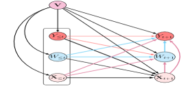
Figure 1: Causal graph over $\mathbf{H}_{t+1}$

Within the framework of Potential Outcome (PO) Rubin [2005], and following Robins and Hernán [2009b], we track a cohort of individuals (units), $i\in\{1,2,\dots,N\}$, over $t_{max}$ sequential time steps. At each time $t\in\{1,2,\dots,t_{max}\}$, we consider: (1) A discrete treatment$W_{it}\in\mathcal{W}=\{0,1,\dots,K-1\}$; e.g., in a medical context, $W_{it}$ may represent radiotherapy and/or chemotherapy. (2) An outcome of interest$Y_{it}\in\mathcal{Y}\subset\mathbb{R}$such as tumor volume. (3) A time-varying context $\mathbf{X}_{it}\in\mathcal{X}\subset\mathbb{R}^{d_{x}}$, containing information about individuals that may explain treatment choice and outcome. $\mathbf{X}_{it}$ is a $d_{x}$-dimensional vector representing confounders. In a medical context, it could include health records and clinical measurements. (4) Static confounders$\mathbf{V}\in\mathcal{V}\subset\mathbb{R}^{d_{v}}$, time-invariant covariates like gender. (5) Partially observed potential outcomes $Y_{it}(\omega_{i,\leq t})$with $\omega_{i,\leq t}:=(\omega_{i,1},\omega_{i,2},\dots,\omega_{i,t})\in\mathcal{W}^{t}$, i.e., outcomes that would have been observed for individual $i$ at time step $t$, had they undergone treatments $\omega_{i,\leq t}$.

We denote $\mathbf{H}_{t+1}=[\mathbf{V},\mathbf{X}_{\leq t+1},W_{\leq t},Y_{\leq t}]$ as the history process up to the assignment of treatment $W_{t+1}$, represented in the causal graph of Figure 1. Given a training dataset $\{\mathbf{H}_{i,t+1},i=1,\dots,N\}$ with an empirical distribution $\mathbb{P}_{\mathbf{H}_{t+1}}$, we address the following causal inference problem: Given a history process $\mathbf{H}_{t+1}$, how can we efficiently estimate counterfactual responses up to $t+\tau$ with $\tau\geq 1$ being the horizon length, for a potential treatment sequence $\omega_{t+1:t+\tau}=(\omega_{t+1},\dots,\omega_{t+\tau})$, i.e., the causal quantity $\mathbb{E}(Y_{t+\tau}(\omega_{t+1},\dots,\omega_{t+\tau})\mid\mathbf{H}_{t+1})$?

We identify the formulated causal quantity from observational data using sequential ignorability Robins and Hernán [2009a], Lim [2018b], Li et al. [2021], Melnychuk et al. [2022], which is implicitly assumed in Figure 1 (details are in Appendix B.1 and B.2). Doing so, we can write:

5 Causal CPC

5.1 Representation learning

Contrastive Predictive Coding. Using contrastive learning, we illustrate how to efficiently learn a representation of the process history $\mathbf{H}_{t}$. Causal forecasting across multiple horizons requires representations with high predictability of variability within $\mathbf{H}_{t}$. In short-term prediction, we aim to capture low-level information and exploit local signal smoothness. For long-term prediction, shared information between history and future points decreases over time, necessitating a more global structure. Capturing long-term dependencies and slow-varying features is crucial in our setting.

Building upon these intuitions, we learn a representation of $\mathbf{H}_{t}$ that is predictive of the encoding of its future components across many time steps, namely the concatenation $\mathbf{U}_{t+j}=[\mathbf{V},\mathbf{X}_{t+j},W_{t+j-1},Y_{t+j-1}]\in\mathcal{U}\subset\mathbb{R}^{(d_{v}+d_{x}+K+1)}$, for $j=1,\dots,\tau$. To do so, we first learn local features by encoding $[\mathbf{V},\mathbf{X}_{t},W_{t-1},Y_{t-1}]$ via $\mathbf{Z}_{t}=\Phi_{\theta_{1}}([\mathbf{V},\mathbf{X}_{t},W_{t-1},Y_{t-1}])$ (architecture details are in Appendix I) and then process all these local features to produce a summary of $\mathbf{H}_{t}$, as in Figure 2, which we call a context representation $\mathbf{C_{t}}$, $\Phi_{\theta_{2}}^{ar}(\mathbf{Z}_{\leq t})=\mathbf{C}_{t}$. $\Phi_{\theta_{2}}^{ar}$ is a simple autoregressive model set in practice to one layer GRU [Cho et al., 2014]. The two resulting encodings give a representation function of the history process $\Phi_{\theta_{1},\theta_{2}}(\mathbf{H}_{t})=\mathbf{C}_{t}$.

We learn a neural network to distinguish, given context $\mathbf{C}_{t}$, future local features $\mathbf{Z}_{t+1},\dots,\mathbf{Z}_{t+\tau}$ related to the same individual from those related to other individuals serving as negative representations. To do so, we minimize the InfoNCE loss $\mathcal{L}^{(InfoNCE)}_{j}$ for each prediction horizon $j$ via

where $\mathcal{B}$ is a batch containing the individual history $\mathbf{H}_{t}$ and $\Gamma_{j}$ is a weight matrix. $T_{j}(.,.)$ is the discriminator of local features at prediction horizon $j$. It pushes the context to predict $\mathbf{U}_{t+j}$ by classifying it among negative samples i.e. the remaining individuals in $\mathcal{B}$. We model $T_{j}$ via Oord et al. [2018]

In practice, the context $\mathbf{C}_{t}$ is used to predict $\mathbf{\hat{Z}}_{t+j}$ (Figure 2), and then the prediction quality is measured with the dot product $\mathbf{Z}_{t+j}^{T}\mathbf{\hat{Z}}_{t+j}$. The information-theoretic interpretation of learning a representation by minimizing $\mathcal{L}^{(InfoNCE)}_{j}$ goes back to the fact that it gives a lower bound to the MI between the context and future local features $I(\mathbf{U}_{t+j},\mathbf{C}_{t})$ Oord et al. [2018]:

$$I(\mathbf{U}_{t+j},\mathbf{C}_{t})\geq\log(|\mathcal{B}|)-\mathcal{L}^{(InfoNCE)}_{j}.$$ (3)

Therefore, for as many forecasting horizons as intended, $j=1,2,\dots,\tau$, we can learn long-term dependencies by minimizing the objectives $\mathcal{L}^{(InfoNCE)}_{j}$ where at each horizon the discriminator parameter matrix $\Gamma_{j}$ is of a small number of dimensions since being a map between two lower-dimensional representations. We, therefore, train $\mathbf{C}_{t}$ to be predictive for large horizon lengths without adding much complexity to the representation by minimizing

We can also trivially write, following the MI lower bounds of Eq. (3), that

Therefore, as we minimize $\mathcal{L}^{CPC}$, we push the model to learn a context representation that shares the maximum information with the future components across all prediction time steps. In this way, we encourage the models to capture the global structure of the process (when $\tau$ is large), which is a very beneficial property for performing counterfactual regression over large horizons.

InfoMax Principle. We introduce a regularization term aiming to make the context representation of the process history $\mathbf{H}_{t}$ "reconstructable." To achieve this, we leverage the InfoMax principle to maximize the MI between $\mathbf{H}_{t}$ and the context $\mathbf{C}_{t}$. However, we avoid computing the contrastive loss between $\mathbf{C}_{t}$ and $\mathbf{H}_{t}$ for two main reasons. First, $\mathbf{H}_{t}$ is a sequence of high-dimensional covariates, and the computation of such loss is computationally demanding. Secondly, we are still interested in incorporating inductive bias toward capturing global dependencies, this time by pushing any subsequence to be predictive of any future subsequence within $\mathbf{H}_{t}$. Hence, we divide the process history into two non-overlapping views, $\mathbf{H}_{t}^{h}:=\mathbf{U}_{1:t_{0}}$, $\mathbf{H}_{t}^{f}:=\mathbf{U}_{t_{0}+1:t}$ representing a historical subsequence and a future subsequence within the process history $\mathbf{H}_{t}$, with $t_{0}$ a randomly chosen splitting time step once per batch. We then maximize the MI between the representations of these views, $\mathbf{C}_{t}^{h}$ and $\mathbf{C}_{t}^{f}$, resulting in a lower bound to the InfoMax objective. Formally,

Proposition 5.1.

$I(\mathbf{C}_{t}^{h},\mathbf{C}_{t}^{f})\leq I(\mathbf{H}_{t},(\mathbf{C}_{t}^{h},\mathbf{C}_{t}^{f}))$.

We provide an intuitive discussion of the inequality by providing an exact writing of the gap in 5.1:

Theorem 5.2.

Both terms on the RHS of Eq. (6) are positive, providing an alternative proof to Proposition 5.1. When equality holds, it implies $I(\mathbf{H}_{t};\mathbf{C}_{t}^{f}\mid\mathbf{C}_{t}^{h})=0$, indicating $\mathbf{H}_{t}$ is independent of $\mathbf{C}_{t}^{f}$ given $\mathbf{C}_{t}^{h}$. This suggests $\mathbf{C}_{t}^{h}$ retains sufficient information from $\mathbf{H}_{t}$ that is predictive of $\mathbf{C}_{t}^{f}$. The symmetry of MI also leads to the occurrence of the second term on the RHS when conditioning on $\mathbf{C}_{t}^{f}$. The equality in Proposition 5.1 implies $\mathbb{P}_{\mathbf{C}_{t}^{h}\mid\mathbf{h}_{t}}=\mathbb{P}_{\mathbf{C}_{t}^{h}\mid\mathbf{c}_{t}^{f}}$, suggesting $\mathbf{C}_{t}^{f}$ efficiently encodes its subsequence while sharing maximum information with $\mathbf{C}_{t}^{h}$.

By considering the proposed variant of the InfoMax principle, we can compute a contrastive bound to $I(\mathbf{C}_{t}^{h},\mathbf{C}_{t}^{f})$ more efficiently, as the random vectors reside in low-dimensional space thanks to the encoding. We define a contrastive loss using InfoNCE similar to Eq. (1):

We use a non-linear discriminator (detailed in Appendix I). The representation of the past subsequence $\mathbf{C}_{t}^{h}$ is mapped to a prediction of the future subsequence $\mathbf{\hat{C}}_{t}^{f}:=F_{\gamma}(\mathbf{C}_{t}^{h})$ and $T_{\gamma}=\mathbf{C}_{t}^{f^{\intercal}}\mathbf{\hat{C}}_{t}^{f}$.

The “mental model" behind our regularization term comes from the MI $I(\mathbf{H}_{t},(\mathbf{C}_{t}^{h},\mathbf{C}_{t}^{f}))$, which we can write using entropy formulation: $I(\mathbf{H}_{t},(\mathbf{C}_{t}^{h},\mathbf{C}_{t}^{f}))=H(\mathbf{H}_{t})-H(\mathbf{H}_{t}\mid(\mathbf{C}_{t}^{h},\mathbf{C}_{t}^{f}))$ . Since the entropy term is constant and parameter-free, the conditional entropy $H(\mathbf{H}_{t}\mid(\mathbf{C}_{t}^{h},\mathbf{C}_{t}^{f}))\geq 0$ is minimized if $\mathbf{H}_{t}$ is a function of $(\mathbf{C}_{t}^{h},\mathbf{C}_{t}^{f})$ almost surely. The theoretical existence of such a function, when the MI is maximized, points to the possibility of decoding the learned context $\mathbf{C}_{t}$ and reconstructing $\mathbf{H}_{t}$.

Beyond the idea of reconstruction, it was shown that the InfoNCE objective implicitly learns to invert the data’s generative model under mild assumptions Zimmermann et al. [2021]. Recent works [Daunhawer et al., 2023, Liu et al., 2024] extend this insight to multi-modal settings, which can reframe our InfoMax problem: $\mathbf{H}_{t}^{h}$ and $\mathbf{H}_{t}^{f}$ can be seen as two coupled modalities, allowing us to identify latent generative factors up to some mild indeterminacies (e.g rotations, affine mappings). We plan to extend multi-modal causal representation learning to the longitudinal setting, where we anticipate minimizing our InfoMax objective, in the limit of infinite data, will effectively invert the data generation process up to a class of indeterminacies that we conjecture to be broader and under weaker assumptions than those in current causal representation learning literature, given our focus is on causal inference rather than the strong identification of causal latent variables.

5.2 Balanced representation learning

We now address selection bias by leveraging the learned context representation $\mathbf{C}_{t}$ of $\mathbf{H}_{t}$. We devise two sub-networks, one for predicting responses and one for predicting treatment; both sub-networks take as input a mapping of the context representation:

$$\mathbf{\Phi}_{t}=\text{SELU}(\text{Linear}(\mathbf{C}_{t}))=\Phi_{\theta_{R}}(\mathbf{H}_{t})$$ (8)

where SELU denotes the Scaled Exponential Linear Unit [Klambauer et al., 2017], and $\theta_{R}$ represents all the parameters of the representation learner. Similar to [Bica et al., 2020a, Melnychuk et al., 2022], our objective is to learn a representation that predicts the outcome while being balanced across all possible treatment arms. This balance ensures that the induced probability distribution over the space of $\mathbf{\Phi}_{t}$ is the same for all possible treatment choices $W_{t}=0,1,\dots,K-1$. To achieve this, we set up an adversarial game: one network learns a distribution over the next treatment given the representation, while a regularization term over the representation encourages it to be non-predictive of that treatment.

Factual response prediction. Since we intend to predict counterfactual responses for $\tau$ steps ahead in time, we train a decoder to predict the factual responses $Y_{t+1},\dots,Y_{t+\tau}$ given the planned sequence of treatment $(W_{t+1},\dots,W_{t+\tau})$. We minimize the negative conditional likelihood

$$\mathcal{L}_{Y}(\theta_{R},\theta_{Y}) =-\log p_{\theta_{Y}}(y_{t+1:t+\tau}\mid\mathbf{\Phi}_{t},\omega_{t+1:t+\tau})$$ (9)

$$=-\sum_{j=1}^{\tau}\log p_{\theta_{Y}}(y_{t+j}\mid y_{t+1:t+j-1},\mathbf{\Phi}_{t},\omega_{t+1:t+j})$$

We assume Gaussian distribution over the conditional responses $Y_{t+j}\mid Y_{t+1:t+j-1},\mathbf{\Phi}_{t},W_{t+1:t+j}\sim\mathcal{N}(G_{Y}(Y_{t+1:t+j-1},\mathbf{\Phi}_{t},W_{t+1:t+j}),\sigma^{2})$, where $G_{Y}$ is a non-linear function that models the mean of the conditional response (see right side of Figure 2). We set $\sigma$ to $\sigma=0.05$ throughout our experiments. The sequence of responses is estimated autoregressively using a GRU-based decoder without teacher forcing Williams and Zipser [1989] to make model training consistent with testing in real-world scenarios (see Figure 2 and Algorithm 2 in Appendix H).

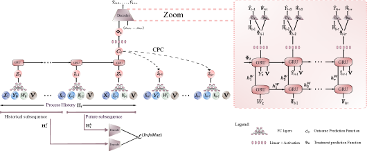
Figure 2: Causal CPC architecture: On the left, a description of the encoder architecture which learns a context $\mathbf{C}_{t}$ from the process history $\mathbf{H}_{t}$, and then two contrastive mechanisms are employed as pretraining: CPC and InfoMax objective. On the right, a decoder takes as an input a mapping of $\mathbf{C}_{t}$ to predict, autoregressively, the future sequence of outcome

Treatment prediction. We learn a treatment prediction sub-network parameterized by $\theta_{W}$ that takes as input the representation $\mathbf{\Phi}_{t+1}$ and predicts a distribution $q_{\theta_{W}}(\omega_{t+1}\mid\mathbf{\Phi}_{t+1})$ over the treatment $W_{t+1}$ by minimizing the negative loglikelihood $\mathcal{L}_{W}=-\log q_{\theta_{W}}(\omega_{t+1}\mid\mathbf{\Phi}_{t+1})$. To assess the quality of the representation in predicting the treatment, the gradient from $\mathcal{L}_{W}$ only updates the treatment network parameters $\theta_{W}$ and is not backpropagated through the response of the parameters for the representation $\mathbf{\Phi}_{t+1}$ (see algorithm 2, Appendix H).

Balanced representation. To create an adversarial game, we update the representation learning parameters, and in the next step, the treatment network $q_{\theta_{W}}(\mid\mathbf{\Phi}_{t+1})$ with adverse losses such that the representation $\mathbf{\Phi}_{t+1}$ becomes invariant w.r.t the assignment of $W_{t+1}$. Different from SOTA models (as highlighted in related work) and in line with our information guidelines principles, learning balanced representation $\Phi_{t+1}$ amounts to ensure $\mathbf{\Phi}_{t+1}\perp\!\!\!\perp W_{t+1}$ which is equivalent to $I(\mathbf{\Phi}_{t+1},W_{t+1})=0$. Hence, we minimize the MI as a way to confuse the treatment classifier. We actually minimize an upper bound over $I(\mathbf{\Phi}_{t+1},W_{t+1})$, namely the CLUB of MI [Cheng et al., 2020]. $\displaystyle I_{\text{CLUB}}(\Phi(\mathbf{H}_{t}),W_{t+1};q_{\theta_{W}})$ $\displaystyle:=\mathbb{E}_{\mathbb{P}_{(\Phi(\mathbf{H}_{t}),W_{t+1})}}\left[\log q_{\theta_{W}}(W_{t+1}\mid\Phi(\mathbf{H}_{t+1}))\right]$ $\displaystyle\quad-\mathbb{E}_{\mathbb{P}_{\Phi(\mathbf{H}_{t})}}\mathbb{E}_{\mathbb{P}_{W_{t+1}}}\left[\log q_{\theta_{W}}(W_{t+1}\mid\Phi(\mathbf{H}_{t+1}))\right].$ (10) We use the objective in Eq. (2) to update the representation learner $\Phi(.)$ Brakel and Bengio [2017], Hjelm et al. [2019]. This update aims to minimize the discrepancy between the conditional likelihood of treatments for units sampled from $\mathbb{P}_{(\mathbf{H}_{t},W_{t+1})}$ and the conditional likelihood of treatments under the assumption of independent sampling from the product of marginals $\mathbb{P}_{\mathbf{H}_{t+1}}\otimes\mathbb{P}_{W_{t+1}}$. In practice, we generate samples from the product of marginals by shuffling the treatment $W_{t+1}$ across the batch dimension similar to Brakel and Bengio [2017], Hjelm et al. [2019].

When minimizing $\mathcal{L}_{W}$, $q_{\theta_{W}}(\omega_{t+1}\mid\mathbf{\Phi}_{t+1})$ gets closer to the true conditional distribution $p(\omega_{t+1}\mid\mathbf{\Phi}_{t+1})$, and, in this case, the objective in Eq. (2) provides an upper bound of the MI between representation and treatment. We formalize the intuition by adapting the result of Cheng et al. [2020]:

Theorem 5.3.

Cheng et al. [2020]
Let $q_{\theta_{W}}(\mathbf{\Phi}_{t+1},\omega_{t+1}):=q_{\theta_{W}}(\omega_{t+1}|\mathbf{\Phi}_{t+1})p(\mathbf{\Phi}_{t+1})$ be the joint distribution induced by $q_{\theta_{W}}(\omega_{t+1}|\mathbf{\Phi}_{t+1})$ over the representation space of $\mathbf{\Phi}_{t+1}$. If:

then $I(\mathbf{\Phi}_{t+1},W_{t+1})\leq I_{CLUB}(\mathbf{\Phi}_{t+1},W_{t+1};q)$

Based on Theorem 5.3, our adversarial training is interpretable and can be explained as follows: the treatment classifier seeks to minimize $\mathbb{E}_{\mathbb{P}_{(\mathbf{H}_{t},W_{t+1})}}\left[\mathcal{L}_{W}\right]$, which is equivalent to minimizing Kullback-Leibler divergence $D_{KL}(p(\mathbf{\Phi}_{t+1},\omega_{t+1})||q_{\theta_{W}}(\mathbf{\Phi}_{t+1},\omega_{t+1}))$. Therefore, $q_{\theta_{W}}(\mathbf{\Phi}_{t+1},\omega_{t+1})$ could get closer to $p(\mathbf{\Phi}_{t+1},\omega_{t+1})$ than, ultimately, to $p(\mathbf{\Phi}_{t+1})p(\omega_{t+1})$, as we train the network to predict $W_{t+1}$ from $\mathbf{\Phi}_{t+1}$. In such a case, $I_{CLUB}$ provides an upper bound on the MI according to theorem 5.3. Hence, in a subsequent step, we minimize $I_{CLUB}$ w.r.t the representation parameters, minimizing the MI $I(\mathbf{\Phi}_{t+1},W_{t+1})$ and achieving balance.

We theoretically formulate such behavior by proving in the following theorem that, at the Nash equilibrium of this adversarial game, the representation is exactly balanced across the different treatment regimes provided by $W_{t+1}$.

Theorem 5.4.

Let $t\in\{1,2,\dots,t_{max}\}$, $\mathbf{\Phi}=\mathbf{\Phi}_{\theta_{R}}$ and $q=q_{\theta_{W}}$ are, respectively, any representation and treatment network. Let $\mathbb{P}_{\mathbf{\Phi}(\mathbf{H}_{t})}$ be the probability distribution over the representation space and $\mathbb{P}_{\mathbf{\Phi}(\mathbf{H}_{t})\mid W_{t+1}}$ its conditional counterpart. Then, there exist $\Phi^{*}$ and $q^{*}$ such that:

$$\Phi^{*} =\arg\min_{\Phi}I_{\text{CLUB}}(\Phi(\mathbf{H}_{t}),W_{t+1};q^{*})$$ (11)

$$q^{*} =\arg\max_{q}\mathbb{E}_{\mathbb{P}_{\Phi^{*}(\mathbf{H}_{t})}}\left[\log q(W_{t+1}\mid\Phi^{*}(\mathbf{H}_{t}))\right]$$

Such an equilibrium holds if and only if $\mathbb{P}_{\mathbf{\Phi}(\mathbf{H}_{t})\mid W_{t+1}=0}=\mathbb{P}_{\mathbf{\Phi}(\mathbf{H}_{t})\mid W_{t+1}=1}=\dots=\mathbb{P}_{\mathbf{\Phi}(\mathbf{H}_{t})\mid W_{t+1}=k-1}$, almost surely.

5.3 Causal CPC training

The Causal CPC model is trained in two stages: (1) Encoder pretraining:we learn an efficient representation of the process history by minimizing the contrastive loss terms $\mathcal{L}_{enc}=\mathcal{L}^{CPC}(\theta_{1},\theta_{2},\{\Gamma_{j}\}_{j=1}^{\tau})+\mathcal{L}^{(InfoMax)}(\theta_{1},\theta_{2},\gamma)$ (2) Decoder training: we train the factual outcome and treatment networks using the adversarial game defined in Theorem 5.4 while fine-tuning the encoder pretrained at the first stage. Formally: $\begin{aligned} &\min_{\theta_{R},\theta_{Y}}\mathcal{L}_{dec}(\theta_{R},\theta_{Y},\theta_{W})=\mathcal{L}_{Y}(\theta_{R},\theta_{Y})+I_{\text{CLUB}}(\Phi_{\theta_{R}}(\mathbf{H}_{t}),W_{t+1};q_{\theta_{W}})\\ &\min_{\theta_{W}}\mathcal{L}_{W}(\theta_{W},\theta_{R})=-\mathbb{E}_{\Phi_{\theta_{R}}(\mathbf{H}_{t})}\left[\log q_{\theta_{W}}(W_{t+1}\mid\Phi_{\theta_{R}}(\mathbf{H}_{t}))\right]\end{aligned}$

6 Experiments

We compare Causal CPC to SOTA baselines: MSMs Robins et al. [2000], RMSN Lim [2018a], CRN Bica et al. [2020a], G-Net Li et al. [2021] and CT Melnychuk et al. [2022]. All the discussed models are fine-tuned by performing a grid search of hyperparameters (architecture and optimizers). The selection criterion is the MSE over factual outcomes on a validation dataset. The same criterion is used for the early stopping strategy for all models’ training. We provide more details on hyperparameters and training in Appendix J and D, respectively.

6.1 Experiments with synthetic data

Tumor Growth. We use the PharmacoKinetic-PharmacoDynamic model in Geng et al. [2017] to predict non-small cell lung cancer patients’ responses to treatments Lim [2018a], Bica et al. [2020a], Melnychuk et al. [2022]. Our approach, similar to Lim [2018a], Bica et al. [2020a], Melnychuk et al. [2022], is evaluated on simulated counterfactual trajectories. We vary the confounding level with a parameter $\gamma$ (additional details are in Appendix E.1). We conduct experiments with fewer patients, 1000 for training and 500 for testing, in contrast to Melnychuk et al. [2022], which used 10,000 for training and 1,000 for testing. This reflects real-world scenarios with limited labeled data, assessing our model’s generalization capabilities.

Results. We run all the models over cancer simulation data for three levels of confounding $\gamma=1,2,3$. Figure 3 shows the evolution of Normalized Root Mean Squared Error (NRMSE) over the counterfactual tumor volume as the forecasting horizon gets larger. The Causal CPC consistently outperforms all the baselines across different levels of confounding, especially at larger prediction horizons, showcasing our model’s effectiveness at long-term predictions. This indicates the quality of representation of $\mathbf{H}_{t}$ at predicting the encoding of its future components across multiple time steps, enabling us to capture the global structure of the process as pointed out by the discussion of Eq. (5). Extended experimental results are in Appendix E.2.1.

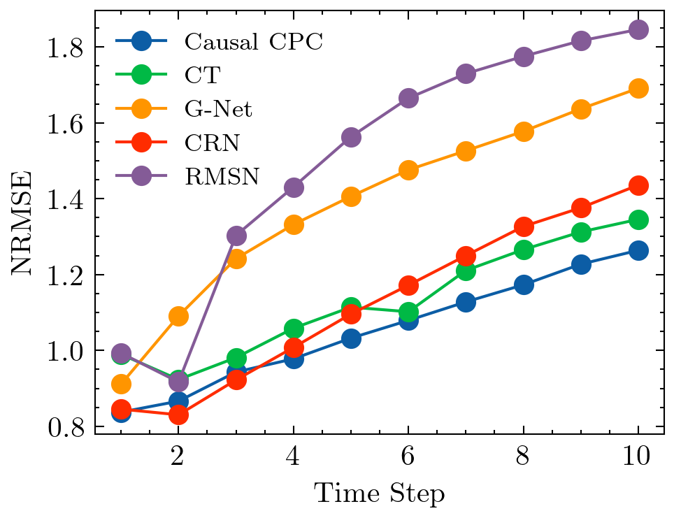
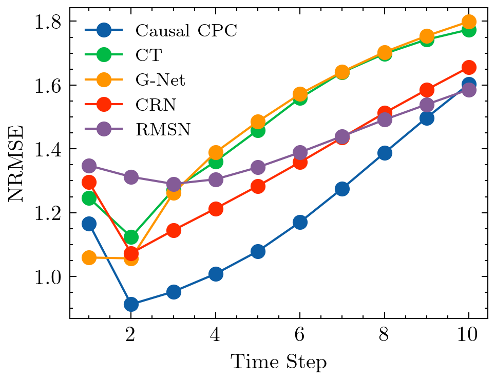
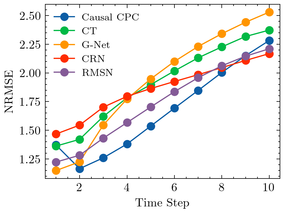
Figure 3: Evolution of error (NRMSE) at estimating counterfactual responses for cancer simulation data for multiple time horizons $\tau=1,2,\dots,10$. On the left, confounding level $\gamma=1$, in the middle $\gamma=2$, and on the right $\gamma=3$. MSM is excluded for its high prediction errors.

6.2 Experiments with semi-synthetic data

Semi-synthetic MIMIC-III. We used a semi-synthetic dataset constructed by Melnychuk et al. [2022] based on the MIMIC-III dataset Johnson et al. [2016], incorporating both endogenous dependencies on time and exogenous dependencies on observational patient trajectories, as detailed in Appendix F.1. The patient trajectories are high-dimensional and exhibit long-range dependencies. Similar to the cancer simulation, training data consisted of relatively few sequences (500 for training, 100 for validation, and 400 for testing). Table 1 presents the mean and standard deviation of counterfactual predictions at multiple horizons ($1\leq\tau\leq 10$). Causal CPC consistently outperformed the baselines, particularly at larger horizons. Additionally, we conducted tests in a setting similar to Melnychuk et al. [2022], where the number of individuals in the training/validation/testing sets was 800/200/200, respectively (Appendix F.2.2), achieving state-of-the-art results, comparable to CT, but with significantly shorter training and prediction times.

Table 1: Results on the MIMIC III semi-synthetic reported by RMSEs. Smaller is better.

Model	$\tau=1$	$\tau=2$	$\tau=3$	$\tau=4$	$\tau=5$	$\tau=6$	$\tau=7$	$\tau=8$	$\tau=9$	$\tau=10$
Causal CPC (ours)	0.32$\pm 0.04$	0.45$\pm 0.08$	0.54$\pm 0.06$	0.61 $\pm 0.10$	0.66$\pm$ 0.10	0.69$\pm$0.11	0.71$\pm$ 0.11	0.73$\pm$ 0.06	0.75 $\pm$ 0.05	0.77$\pm$ 0.10
Causal Transformer	$0.42\pm 0.38$	0.40$\pm$ 0.06	0.52$\pm$ 0.08	0.60$\pm$ 0.005	0.67$\pm 0.10$	0.72 $\pm 0.12$	0.77$\pm 0.13$	0.81$\pm 0.14$	0.85 $\pm 0.16$	0.88 $\pm$0.17
G-Net	$0.54\pm 0.13$	0.72$\pm 0.14$	0.85 $\pm$0.16	0.96 $\pm$ 0.17	1.05 $\pm$ 0.18	1.14 $\pm$0.18	1.24$\pm$ 0.17	1.33$\pm 0.16$	1.41 $\pm$ 0.16	1.49$\pm$0.16
CRN	0.27 $\pm$0.03	0.45$\pm 0.08$	0.58 $\pm$ 0.09	0.72$\pm$ 0.11	0.82$\pm$ 0.15	0.92 $\pm$ 0.20	1.00 $\pm$ 0.25	1.06 $\pm$ 0.28	1.12 $\pm$ 0.32	1.17 $\pm$ 0.35
RMSN	0.40 $\pm$ 0.16	0.70 $\pm$ 0.21	0.80$\pm$ 0.19	0.88 $\pm$ 0.17	0.94 $\pm$ 0.16	1.00 $\pm$ 0.15	1.05 $\pm$ 0.14	1.10 $\pm$ 0.14	1.14 $\pm$ 0.13	1.18 $\pm$ 0.13

Computational Efficiency and Model Complexity. Efficient execution is crucial for practical deployment, especially with periodic retraining. Computational considerations extend beyond training, especially when evaluating multiple counterfactual trajectories per individual. The maximum number of counterfactual trajectories per individual starting from a current time step is determined by $K^{\tau}$, where $K$ represents the number of possible treatments. The exponential growth of these trajectories as the forecasting horizon expands poses a significant computational challenge. This is particularly relevant when generating multiple treatment trajectories to identify the most effective one, such as the trajectory leading to the smallest tumor volume at the end of a treatment plan.

Table 2: The number of parameters for each model and the running time averaged over five seeds. Results are reported for tumor growth simulation ($\gamma=1$). Hardware: GPU-1xNVIDIA Tesla M60.

Model	trainable parameters (k)	Training time (min)	Prediction time (min)
Causal CPC (ours)	8.2	16$\pm$ 3	4 $\pm$ 1
Causal Transformer	11	12$\pm$ 2	30$\pm$ 3
G-Net	1.2	2 $\pm$ 0.5	35 $\pm$ 3
CRN	5.2	13$\pm$ 2	4$\pm$ 1
RMSN	1.6	22$\pm$ 2	4 $\pm$ 1
MSM	$<$0.1	1$\pm$0.5	1$\pm$ 0.5

Table 2 presents the models’ complexity (number of parameters) and running time, divided into model fitting and prediction. Predictions are generated for multiple random treatment plans per individual at all possible starting times (Appendix D). Causal CPC is highly efficient in prediction time due to its simple backbone (1-layer GRU), similar to CRN (1-layer LSTM), but outperforms CRN. Conversely, CT is less efficient at testing due to numerous testing trajectories and transformer architecture, plus being trained using teacher forcing, which requires recursive loading of data to generate sequences at prediction. G-Net exhibits high prediction times due to Monte Carlo sampling. In conclusion, Causal CPC offers a favorable trade-off between prediction quality and running time efficiency.

6.3 Ablation study

Table 3: Ablation study of Causal CPC. We report NRMSE averaged across ($1\leq\tau\leq 10$) for cancer simulation ($\gamma=1$) and MIMIC III.

Model	Cancer_Sim	MIMIC III
Causal CPC (Full)	1.05	0.66
Causal CPC (w/o $\mathcal{L}^{(InfoNCE)}$)	1.07	0.68
Causal CPC (w/o $\mathcal{L}^{(InfoMax)}$)	1.13	0.74
Causal CPC (w CDC loss)	1.07	0.73
Causal CPC (w/o balancing)	1.08	0.69

To show the efficacy of our contrastive terms, we evaluate the model under various configurations: full model, without CPC, and without InfoMax. Table 3 illustrates the drop in counterfactual prediction accuracy averaged across all forecasting horizons, emphasizing the relevance of the two regularization terms. The error increases when replacing our ICLUB objective with CDC loss Melnychuk et al. [2022] and not enforcing balancing. We tested other MI lower bounds for both CPC and InfoMax objectives, namely Nguyen, Wainwright, and Jordan (NWJ) [Nguyen et al., 2010] and Mutual Information Neural Estimator (MINE) Belghazi et al. [2018] (Appendix C.2). InfoNCE loss gives better results for the two objectives (Table 9). Detailed results on the ablation study are in Appendix E.2.2 and F.2.1.

6.4 Falsifiability Test

In this work, we operated under the assumption of sequential ignorability, commonly adopted in similar contexts Lim [2018a], Bica et al. [2020a], Li et al. [2021], Melnychuk et al. [2022]. However, we assess our model’s robustness by conducting a refutability test. We remove some confounders during model training while retaining them in the data construction for MIMIC III. Table 4 presents the mean and standard deviation of predictions of counterfactuals at multiple horizons when sequential ignorability is violated. Compared to Table 1, where assumptions aren’t violated, errors of Causal CPC, Causal Transformer, and CRN increase when some confounders are masked, except RMSN, which remains insensitive during the robustness test. However, RMSN starts underperforming significantly at $\tau\geq 2$. Our model maintains its advantage of outperforming baselines at large horizons even when sequential ignorability is violated, highlighting its ability to effectively encode long-term dependencies of observed confounders.

Table 4: Results on the MIMIC III when sequential ignorability is violated reported by RMSEs

Model	$\tau=1$	$\tau=2$	$\tau=3$	$\tau=4$	$\tau=5$	$\tau=6$	$\tau=7$	$\tau=8$	$\tau=9$	$\tau=10$
Causal CPC	0.44$\pm$ 0.04	0.56$\pm$ 0.07	0.66$\pm 0.07$	0.73 $\pm$ 0.08	0.78$\pm$ 0.08	0.83$\pm$0.06	0.86$\pm$ 0.10	0.88$\pm$ 0.08	0.91 $\pm$ 0.08	0.95$\pm$ 0.07
Causal Transformer	0.34$\pm$0.07	0.48$\pm$0.07	0.60$\pm$0.07	0.68$\pm$0.06	0.75$\pm$ 0.06	0.80$\pm$0.07	0.86$\pm$ 0.09	0.91$\pm 0.11$	0.95 $\pm 0.13$	1.00 $\pm$0.15
CRN	0.40$\pm$ 0.07	0.54$\pm$ 0.09	0.70$\pm$ 0.09	0.84$\pm$ 0.09	0.97$\pm$ 0.09	1.08$\pm$ 0.13	1.18$\pm$ 0.16	1.26$\pm$ 0.19	1.33$\pm$ 0.21	1.39$\pm$ 0.23
RMSN	0.38$\pm$ 0.08	0.67$\pm$ 0.21	0.78$\pm$ 0.16	0.84$\pm$ 0.14	0.91$\pm$ 0.14	0.98$\pm$ 0.15	1.04$\pm$ 0.16	1.09$\pm$ 0.18	1.15$\pm$ 0.19	1.20$\pm$ 0.23

7 Conclusion

Our novel approach to long-term counterfactual regression combines RNNs with CPC, achieving SOTA results without relying on complex transformers. Prioritizing efficiency, we introduce regularizations using contrastive losses. Guided by our MI-based principles, our method outperforms existing models in counterfactual estimation on both synthetic and real-world data, marking the first application of CPC in causal inference. Future research could focus on improving prediction interpretability by potentially integrating Shapley values into counterfactual regression over time. Considering our use of causal graphs, exploring Causal Shapley Values Heskes et al. [2020] could be fruitful for understanding important factors in the confounding process. Additionally, there’s a need for uncertainty-aware models De Brouwer et al. [2022], Jesson et al. [2020], Yin et al. [2024] tailored for longitudinal problems, enhancing reliability and transparency in our causal framework.

Appendix A Impact Statements

Our paper seeks to advance the field of Trustworthy Machine Learning by focusing on the accurate estimation of counterfactual trajectories. This capability holds significant potential to enhance decision-making processes across various domains, particularly in healthcare, where clinicians can leverage models designed to mitigate bias and promote fairness. Additionally, by focusing on efficiency, our contributions extend beyond traditional machine learning considerations to address environmental concerns associated with energy consumption. By advocating for the prudent use of computational resources, especially in training complex models deployed in real-world scenarios, we aim to promote sustainability in developing and applying machine learning solutions.

Appendix B Causal assumptions

B.1 Identifiability Assumptions in Causal CPC

In this section, we detail the assumptions used for the identifiability of the counterfactual responses $\mathbb{E}(Y_{t+\tau}(\omega_{t+1:t+\tau})\mid\mathbf{H}_{t+1})$. As briefly stated in section 3, we follows similar assumptions to Robins and Hernán [2009a], Robins et al. [2000], Bica et al. [2020a], Melnychuk et al. [2022], namely

Assumption B.1 (Consistency).

For every time step $t$ and given any manner by which a unit $i$ receives the sequence of treatment $\omega_{i,\leq t}$, we always observe the potential outcome $Y_{it}(\omega_{i,\leq t})$. Formally:

$$W_{i,\leq t}=w_{i,\leq t}\implies Y_{it}=Y_{it}(w_{i,\leq t}).$$

Assumption B.2 (Sequential Ignorability).

Given any time step t, we have the conditional independence:

$$Y_{it}(\omega_{it})\perp\!\!\!\perp W_{it}|\mathbf{H}_{it}=\mathbf{h}_{it}\quad\forall(\omega_{it},\mathbf{h}_{it})$$

Assumption B.3 (Overlap/positivity).

Given any time step $t$, and for any possible historical context $\mathbf{h}_{t}$, the probability of observing any of the possible treatment regimes is strictly positive but not deterministic:

$$p(\mathbf{h}_{t})\neq 0\implies 0<p(W_{t}=\omega_{t}|\mathbf{h}_{t})<1$$

The three assumptions are sufficient for the identification of the counterfactual responses from observational data, which we formulate in the following proposition.

Proposition B.4.

Assuming consistency, overlap, and ignorability (assumptions B.1, B.2, B.3), the causal quantity $\mathbb{E}(Y_{t+\tau}(\omega_{t+1:t+\tau})\mid\mathbf{H}_{t+1})$ is identifiable from observational data following

$$\mathbb{E}(Y_{t+\tau}(\omega_{t+1:t+\tau})\mid\mathbf{H}_{t+1})=\mathbb{E}\left(Y_{t+\tau}\mid\mathbf{H}_{t+1},W_{t+1:t+\tau}=\omega_{t+1:t+\tau}\right)$$

Proof.

See Robins and Hernán [2009a] ∎

B.2 On the Causal Graph

We repeat the causal graph introduced in Figure 1 to explain the data generation process. here, all of the past observed data encompassed in $\mathbf{H}_{t+1}$ confounds future treatments and responses, $W_{t+1},W_{t+2},\dots,W_{t_{max}}$ and $Y_{t+1},Y_{t+2},\dots,Y_{t_{max}}$, which create long-term dependencies. The fact that post-covariates are affected by past treatments creates time-dependent confounding. The static covariates are assumed to be affecting all of the time-varying variables. Since we suppose sequential ignorability, there are no possible exogenous noises affecting both treatments and responses. However, such noise may possibly affect responses, time-varying covariates, and response variables.

In the figure, for simplicity, we represent past treatments as $W_{\leq t}$ such that each element in that sub-sequence confounds the next treatment and response $W_{t+1}$ and $Y_{t+1}$. Idem for $Y_{\leq t}$ and $\mathbf{X}_{\leq t}$. The static covariates $\mathbf{V}$ are assumed to be affecting all the time-varying variables. We omit the representation of exogenous noise for simplicity. Interactions between $W_{\leq t}$ , $\mathbf{X}_{\leq t}$, and $Y_{\leq t}$ were also omitted for simplicity.

Appendix C Extended related work

C.1 Counterfactual regression over time: Methods overview

C.1.1 Methods included in experiments

In this section, we give a brief overview of models included in our experiments: MSMs Robins and Hernán [2009a], RMSN Lim [2018a], CRN Bica et al. [2020a], G-Net Li et al. [2021], and CT Melnychuk et al. [2022]. To delineate the differences between these models and Causal CPC, we detail in Table 5 the main design differences between all these models.

Table 5: A summary of the methods included in our experiments

Model	Model Backbone	Tailored to long-term forecast?	Learning of long-term dependencies	Use of contrastive learning	Prediction of counterfactuals	handling selection bias	Invertibility of representation
Causal CPC (ours)	GRU	yes	Contrastive Predictive Coding	learn long-term relations	Autoregressive	Balanced representation	yes, contrast representation with input
Causal Transformer	3 Transformers	yes	Transformer architecture	N/A	Autoregressive	Balanced representation	N/A
G-Net	LSTM	No	N/A	N/A	Autoregressive	G-Computation	Current covariates $\mathbf{X}_{t}$
CRN	LSTM	No	N/A	N/A	Autoregressive	Balanced representation	N/A
RMSN	LSTM	No	N/A	N/A	Autoregressive	Weighting	N/A
MSM	Logistic+linear model	No	N/A	N/A	Autoregressive	Weighting	N/A

C.1.2 Methods violating our assumptions

Our work relies on sequential ignorability. However, alternative models presume the presence of unobserved confounders. Some models draw inspiration from deconfounding theory [Lopez and Gutman, 2017, Ranganath and Perotte, 2018, Wang and Blei, 2019], and its recent extensions to time-varying settings. Deconfounding entails imposing a factor model over treatment assignment, where each cause becomes conditionally independent given latent variables that act as substitutes for unobserved confounders. Examples include Bica et al. [2020b], Hatt and Feuerriegel [2021], Cao et al. [2023]. Other models assume the observation of proxy variables, employing probabilistic models to infer a representation for unobserved confounding based on these proxy variables Veitch et al. [2020], Cheng et al. [2021], Kuzmanovic et al. [2021].

In contrast to our setting defined by the three causal assumptions in Appendix B.1, other models operate in a setting where a data-generating model is assumed similar to Soleimani et al. [2017b, a], Qian et al. [2021]. These methods are generally non- or semi-parametric, often either ignoring or linearly accounting for static covariates, besides exhibiting computational inefficiency and struggling to scale to large datasets. Conversely, within the same non- or semi-parametric modeling paradigm, Schulam and Saria [2017], Seedat et al. [2022], De Brouwer et al. [2022], Hızlı et al. [2023] adopt the same causal assumptions as our work, but time is considered continuous, and sequential ignorability extends to continuous time. Additionally, considering continuous time counterfactual outcomes, Jiang et al. [2023] assumes non-independence of units, where units are affected not only by their own treatments but also by those of other individuals.

C.2 Mutual Information and Self-Supervision

Self-Supervised Learning and Mutual Information In the realm of self-supervised learning and mutual information (MI), Deep InfoMax Hjelm et al. [2019] employs MI computation between input images and representations, emphasizing its maximization to enhance reconstruction quality. Additionally, local MI calculations between the representation and local features contribute to encoding more intricate patterns shared across data patches. The strategy of maximizing average MI between the representation and local regions, such as patches, significantly improves downstream task performance. Notably, global MI assumes a more prominent role in reconstructing the complete input given the representation.

CPC aligns with the MI-based approach seen in Deep InfoMax, emphasizing the maximization of MI between global and local representation pairs. Distinct from Deep InfoMax, CPC processes local features sequentially, constructing partial "summary features" to predict specific local features in the future. Classical self-supervised paradigms often focus on tasks like classification or reconstruction-based objectives, leading to distinct preferences for maximizing MI in either local or global information. However, the integration of both procedures becomes imperative in scenarios involving downstream tasks like counterfactual regression over time. Our proposed Causal CPC is strategically designed to align with these intuitions.

Several other methods share similarities with CPC, such as Contrastive Multiview Coding Tian et al. [2020]. This method emphasizes maximizing mutual information between representations of different views of the same observation. Augmented Multiscale Deep InfoMax Bachman et al. [2019], akin to CPC, makes predictions across space but differs by predicting representations across layers in the model. While Instance Discrimination Zhao et al. [2020] encourages representations capable of discriminating between individual examples in the dataset, our preference for CPC arises from its adaptability in processing sequential features in an ordered and autoregressive manner. This aligns seamlessly with the requirements of our specific context, especially when dealing with counterfactual regression over time.

Mutual Information and Inductive Bias. The success of mutual information estimation is not solely dictated by MI’s inherent properties but also by the inductive bias linked to the choice of feature representation and parameterization in the MI estimator Tschannen et al. [2020]. Experimental findings reveal that, although MI is invariant under homeomorphisms, its maximization during random initialization with an invertible encoder leads to improved downstream performance over training. Additionally, higher-capacity critics provide tighter MI bounds, but empirical evidence, consistent with observations by Rainforth et al. [2018] regarding evidence lower bounds in variational problems, indicates that simpler critics yield better representations even with looser MI bounds. This observation guided our selection of a simple bilinear critic function in contrastive losses. In the context of vision problems, besides the theoretical importance of augmentations and contrastive loss properties on representation efficiency for downstream tasks [Arora et al., 2019, Tosh et al., 2021, HaoChen et al., 2021], Saunshi et al. [2022] underscores the impact of inductive bias (function class representation and optimizers) on downstream performance and proposed in this case, theoretical, non-vacuous guarantees on the representation efficiency.

Variational Approaches and MI Estimation Challenges The estimation of MI faces inherent challenges, particularly within variational lower bounds. These bounds often degrade as MI increases, creating a delicate trade-off between high bias and high variance. To address this, methods that utilize upper bounds on MI have been developed, attempting to mitigate challenges associated with variational bounds. One strategy for MI maximization involves computing gradients of a lower MI bound concerning the parameters of a stochastic encoder. This computational approach potentially eliminates the need for direct MI estimation, providing a more tractable solution. However, estimating MI from samples remains challenging, and traditional approaches encounter scalability issues in modern machine-learning problems.

It’s crucial to note that higher estimated MI between observations and learned representations does not consistently translate to improved predictive performance in downstream supervised learning tasks. CPC is an example, exhibiting less variance but more bias, with estimates capped at $\log|\mathcal{B}|$. Strategies to reduce bias, such as increasing the batch size, introduce higher computational complexity, requiring additional evaluations for estimating each batch with the encoding function.

In our empirical approach, we adopt a specific sampling strategy for sequences, considering a one-time step per batch. This facilitates computing the InfoNCE between local summary features at time t and the future prediction of local features, leading to a reduction in algorithmic complexity for contrastive loss computation. Empirical observations demonstrate non-decreased representation quality and improved prediction of factual and counterfactual outcomes. Other MI lower bounds. The Mutual Information Neural Estimator (MINE) Belghazi et al. [2018] leverages the relationship between MI and the Kullback-Leibler (KL) divergence. MI can be expressed as the KL divergence between the joint distribution and the product of marginals:

$$I(X;Z):=D_{KL}(\mathbb{P}_{(X,Z)}||\mathbb{P}_{X}\otimes\mathbb{P}_{Z})$$

MINE employs the Donsker-Varadhan representation Donsker and Varadhan [1983] of the KL divergence:

$$D_{KL}(\mathbb{P}\,||\,\mathbb{Q})=\sup_{T:\Omega\rightarrow\mathbb{R}}E_{\mathbb{P}}[T]-\log\left(E_{\mathbb{Q}}[e^{T}]\right)$$ (12)

Here, the supremum is over all functions $T$ where the expectations exist. For a specific class of functions $\mathcal{F}$, potentially represented by a class of neural networks, we obtain the lower bound:

$$D_{KL}(\mathbb{P}\,||\,\mathbb{Q})\geq\sup_{T\in\mathcal{F}}E_{\mathbb{P}}[T]-\log\left(E_{\mathbb{Q}}[e^{T}]\right)$$ (13)

In practice, we maximize $\hat{I}^{MINE}_{\gamma}(\mathbb{P}\,||\,\mathbb{Q})=E_{\mathbb{P}}[T_{\gamma}]-\log(E_{\mathbb{Q}}[e^{T_{\gamma}}])$, where $T_{\gamma}$ is a discriminator parameterized by $\gamma$, representing neural network parameters. The MINE estimator has the property of being a strongly consistent estimator of the true MI (Theorem 2 Belghazi et al. [2018]).

Alternatively, the f-divergence representation of $D_{KL}$ Nowozin et al. [2016] allows us to derive another lower bound on MI known as Nguyen, Wainwright, and Jordan (NWJ) [Nguyen et al., 2010]:

$$D_{KL}(\mathbb{P}\,||\,\mathbb{Q})\geq\sup_{T\in\mathcal{F}}E_{\mathbb{P}}[T]-\log\left(E_{\mathbb{Q}}[e^{T-1}]\right)$$ (14)

This results in the estimator $\hat{I}^{NWJ}_{\gamma}(\mathbb{P},\mathbb{Q})=E_{\mathbb{P}}[T_{\gamma}]-\log(E_{\mathbb{Q}}[e^{T_{\gamma}-1}])$. Unlike the InfoNCE estimator, which exhibits a high bias and a low variance, the NWJ estimator has a low bias but a high variance Poole et al. [2019b].

Appendix D Experimental protocol

All models were implemented using PyTorch Paszke et al. [2019] and PyTorch Lightning [Falcon and The PyTorch Lightning team, 2019]. In contrast to the approach in Melnychuk et al. [2022], we employed early stopping for all models. The stopping criterion was defined as the Mean Squared Error over factual outcomes for a dedicated validation dataset. Specifically, for the Causal CPC encoder, the stopping criterion was determined by the validation loss of the encoder.

While all models in the benchmark were trained using the Adam optimizer Kingma and Ba [2014], we opted for training Causal CPC (encoder plus decoder without the treatment subnetwork) with AdamW Loshchilov and Hutter [2017] due to its observed stability during training. Similar to the common practice in training GAN discriminators, the treatment subnetwork was optimized using SGD with momentum Sutskever et al. [2013].

The CT employed the Exponential Moving Average (EMA) Yazıcı et al. [2019] of parameters to enhance training stability. However, this technique was not applied to Causal CPC, as experimental evidence suggested only marginal improvements. Weight decay was set to zero for all models.

For each experiment, the models were trained over five different seeds, and the reported performance metrics include the mean and standard deviation of the results.

The counterfactual trajectories are generated following two strategies:

• Single sliding treatment [Bica et al., 2020a, Melnychuk et al., 2022]: Trajectories are generated with a single treatment per trajectory while the treatment slides over the forecasting range to generate multiple trajectories. Similar to Bica et al. [2020a], we apply such a generation scheme to cancer simulation data.

• Random trajectories: Trajectories are generated such that at each time step, treatment is generated randomly. We apply random trajectories to semi-synthetic MIMIC data.

For the falsifiability test on MIMIC III datset, we mask two confounders from the inputs of the benchmark models, namely sodium and glucose measurements.

Appendix E Experiments on synthetic data: Details

E.1 Description of the simulation model

We present a tumor growth simulation model. Specifically, we focus on the PharmacoKinetic-PharmacoDynamic (PK-PD) model, as discussed in Geng et al. [2017], which is a recent model used to predict treatment responses in non-small cell lung cancer patients. In this simulation, we model the evolution of tumor volume, denoted as $V(t)$, in discrete time, with $t$ representing the number of days since diagnosis:

$$V(t)=\left(1+\underbrace{\Lambda\log\left(\frac{K}{V(t-1)}\right)}_{\text{Tumor Growth}}-\underbrace{\kappa_{c}C(t)}_{\text{Chemotherapy}}-\underbrace{\left(\kappa_{rd}Rd(t)+\upsilon Rd(t)^{2}\right)}_{\text{Radiation}}+\underbrace{e_{t}}_{\text{Noise}}\right)V(t-1)$$

Here, the model parameters $\Lambda,K,\kappa_{c},\kappa_{rd},\upsilon$ are sampled for each patient based on prior distributions from Geng et al. [2017]. Additionally, $Rd(t)$ represents the radiation dose applied at time $t$, and $\mathrm{C}(t)$ denotes the drug concentration.

We introduce confounding into the assignment of radiotherapy/chemotherapy treatment by making it dependent on the past tumor volume evolution. Treatment is simulated using a Bernoulli distribution with probability $\sigma(\pi_{t})$, where:

$$\pi_{t}=\frac{\gamma}{D_{\max}}\left(\bar{D}(t)-\delta\right)$$

Here, $\bar{D}(t)$ represents the average tumor diameter over the last 15 days, and $D_{\max}=13~{}\mathrm{cm}$ is the maximum tumor diameter. The parameter $\delta$ is set to $\delta=D_{\max}/2$. The parameter $\gamma$ controls the level of time-dependent confounding; a higher value of $\gamma$ gives more weight to the history of tumor diameter in treatment assignment.

E.2 Additional results

E.2.1 Comparison to benchmark models

We report in this section detailed counterfactual errors for Causal CPC and baselines over the cancer simulation dataset, which are responsible for Figure 3.

Table 6: Results on the synthetic data set: mean$\pm$standard deviation of Normalized Rooted Mean Squared Errors (NRMSEs). The best value for each metric is given in bold: smaller is better.

$\gamma=1$
Model	$\tau=1$	$\tau=2$	$\tau=3$	$\tau=4$	$\tau=5$	$\tau=6$	$\tau=7$	$\tau=8$	$\tau=9$	$\tau=10$
Causal CPC (ours)	0.83$\pm$ 0.06	0.86 $\pm$ 0.09	0.94$\pm$ 0.09	0.97$\pm$ 0.08	1.03$\pm$ 0.10	1.07 $\pm$ 0.10	1.12$\pm$ 0.10	1.17 $\pm$ 0.09	1.22$\pm$ 0.08	1.26$\pm$ 0.08
Causal Transformer	0.99$\pm$ 0.13	0.92 $\pm$ 0.14	0.98$\pm$ 0.14	1.05$\pm$ 0.15	1.11 $\pm$ 0.18	1.11 $\pm 0.11$	1.21 $\pm$ 17	1.26$\pm$ 0.16	1.31 $\pm$ 0.005	1.35$\pm$ 0.16
G-Net	0.91$\pm$0.15	1.1$\pm$0.16	1.24$\pm$0 16	1.33$\pm$0.17	1.40$\pm$0.18	1.47$\pm$0.19	1.52$\pm$0.18	1.57$\pm$0.22	1.63$\pm$0.22	1.7$\pm$0.25
CRN	0.84$\pm$0.10	0.83$\pm$0.09	0.92$\pm$0.10	1.00$\pm$0.11	1.09$\pm$0.12	1.17$\pm$0.14	1.25$\pm$0.16	1.32$\pm$0.18	1.37$\pm$0.23	1.43$\pm$0.26
RMSN	0.99$\pm$0.13	0.91$\pm$0.04	1.30$\pm$0.65	1.43$\pm$0.76	1.56$\pm$0.83	1.66$\pm$0.88	1.73$\pm$0.91	1.77$\pm$0.89	1.81$\pm$0.88	1.84$\pm$0.86
MSM	1.20$\pm$0.10	1.83$\pm$0.26	2.07$\pm$0.44	2.38$\pm$0.44	2.54$\pm$0.45	2.90$\pm$0.37	3.01$\pm$.38	3.06$\pm$0.36	3.08$\pm$0.36	3.08$\pm$0.36
$\gamma=2$
Causal CPC (ours)	1.16$\pm$ 0.22	0.91 $\pm$ 0.10	0.95 $\pm$ 0.13	1.00 $\pm$ 0.15	1.07$\pm$ 0.19	1.17 $\pm$ 0.24	1.27 $\pm$ 0.25	1.38 $\pm$ 0.28	1.49 $\pm$ 0.30	1.60 $\pm$ 0.34
Causal Transformer	1.24$\pm$0.20	1.13$\pm$0.15	1.27$\pm$021	1.36$\pm$0.28	1.44$\pm$0.29	1.55$\pm$0.27	1.64$\pm$0.28	1.69$\pm$0.20	1.74$\pm$0.28	1.77 $\pm$ 0.29
G-Net	1.05$\pm$0.21	1.05$\pm$0.08	1.26$\pm$0.16	1.38$\pm$0.23	1.48$\pm$0.27	1.57$\pm$0.31	1.64$\pm$0.33	1.70$\pm$0.36	1.75$\pm$0.39	1.8$\pm$0.42
CRN	1.25$\pm$0.25	1.08$\pm$0.06	1.14$\pm$0.12	1.21$\pm$0.17	1.30$\pm$ 0.21	1.41$\pm$0.25	1.54$\pm$0.32	1.67$\pm$0.41	1.8$\pm$0.51	1.92$\pm$0.63
RMSN	1.47$\pm$0.27	1.33$\pm$0.25	1.30$\pm$0.23	1.33$\pm$0.24	1.38$\pm$0.26	1.45$\pm$0.28	1.52$\pm$0.31	1.60$\pm$0.25	1.67$\pm$0.38	1.75$\pm$0.42
MSM	1.43$\pm$0.27	2.22$\pm$0.53	2.67$\pm$0.63	2.98$\pm$0.70	3.19$\pm$0.74	3.33$\pm$0.77	3.41$\pm$0.79	3.44$\pm$0.25	3.45$\pm$0.78	3.34$\pm$0.77
$\gamma=3$
Causal CPC (ours)	1.37$\pm$0.31	1.16$\pm$0.27	1.26$\pm$0.30	1.38$\pm$0.35	1.53$\pm$0.40	1.69$\pm$0.47	1.84$\pm$0.52	2.00$\pm$0.51	2.14$\pm$0.61	2.28$\pm$0.66
Causal Transformer	1.36$\pm$0.32	1.42$\pm$0.36	1.62$\pm$0.46	1.78$\pm$0.53	1.89$\pm$0.58	2.01$\pm$0.63	2.13$\pm$0.66	2.22$\pm$0.69	2.31$\pm$0.69	2.37$\pm$0.73
G-Net	1.14$\pm$0.24	1.22$\pm$0.15	1.54$\pm$0.26	1.77$\pm$0.33	1.94$\pm$0.36	2.09$\pm$0.40	2.23$\pm$0.43	2.34$\pm$0.47	2.44$\pm$0.52	2.52$\pm$0.56
CRN	1.46$\pm$0.29	1.54$\pm$0.38	1.70$\pm$0.48	1.79$\pm$0.53	1.86$\pm$0.92	1.92$\pm$0.58	1.98$\pm$0.59	2.04$\pm$0.61	2.10$\pm$0.63	2.16$\pm$0.64
RMSN	1.22$\pm$0.26	1.28$\pm$0.29	1.43$\pm$0.40	1.56$\pm$0.48	1.70$\pm$0.53	1.83$\pm$0.57	1.95$\pm$0.59	2.06$\pm$0.61	2.14$\pm$0.61	2.21$\pm$0.61
MSM	1.70$\pm$0.35	2.73$\pm$0.88	3.22$\pm$1.03	3.25$\pm$1.12	3.71$\pm$1.18	3.85$\pm$1.22	3.91$\pm$1.23	3.95$\pm$1.24	3.96$\pm$1.24	3.94$\pm$1.23

E.2.2 Ablation study

We detail here the results of the ablation study conducted on the cancer simulation dataset (Table 3). The (full) Causal CPC model, as presented in the core paper, gives, in most cases, better results than any ablation configuration.

Table 7: Results of the ablation study on the synthetic data set: mean$\pm$standard deviation of Normalized Rooted Mean Squared Errors (NRMSEs). The best value for each metric is given in bold: smaller is better.

Model	$\tau=1$	$\tau=2$	$\tau=3$	$\tau=4$	$\tau=5$	$\tau=6$	$\tau=7$	$\tau=8$	$\tau=9$	$\tau=10$
CAUSAL CPC (FULL)	0.83 $\pm$ 0.06	0.86 $\pm$ 0.06	0.94$\pm$ 0.09	0.97 $\pm$ 0.08	1.03 $\pm$ 0.10	1.07$\pm$0.10	1.12$\pm$ 0.10	1.17$\pm$ 0.06	1.22 $\pm$ 0.08	1.26$\pm$ 0.08
Causal CPC (w/o $\mathcal{L}^{(InfoNCE)}$)	0.84$\pm$0.04	0.91$\pm$0.07	0.95$\pm$ 0.07	0.99$\pm$ 0.09	1.03$\pm$0.10	1.10$\pm$ 0.07	1.15$\pm 0.14$	1.20 $\pm$ 0.14	1.23$\pm$0.14	1.28$\pm 0.15$
Causal CPC (w/o $\mathcal{L}^{(InfoMax)}$)	0.84$\pm$0.04	0.86$\pm$0.09	0.91$\pm$0.08	0.99$\pm$0.10	1.07$\pm$0.08	1.16$\pm$ 0.08	1.24$\pm$ 0.10	1.31 $\pm$ 0.12	1.38$\pm$0.08	1.46$\pm 0.10$
Causal CPC (w CDC loss)	0.83$\pm$0.02	0.89$\pm$0.07	0.96$\pm$ 0.07	1.03$\pm$ 0.07	1.07$\pm$0.08	1.10$\pm$ 0.07	1.13$\pm 0.10$	1.18 $\pm$ 0.09	1.24$\pm$0.11	1.28$\pm 0.11$
Causal CPC (w Balancing	0.84$\pm$0.04	0.88$\pm$0.05	0.97$\pm$ 0.05	1.04$\pm$ 0.07	1.08$\pm$0.10	1.13$\pm$ 0.08	1.15$\pm 0.14$	1.20$\pm$ 0.10	1.25$\pm$0.08	1.29$\pm 0.12$

Appendix F Experiments on semi-synthetic data: Details

F.1 Description of the simulation model

In this section, we provide a concise overview of the simulation model built upon the MIMIC III dataset introduced by Melnychuk et al. [2022]. Initially, a cohort of 1,000 patients is extracted from the MIMIC III data, and the simulation proposed by Melnychuk et al. [2022] extends that of Schulam and Saria [2017].

Let $d_{y}$ be the dimension of the outcome variable, in the case of multiple outcomes, then untreated outcomes, denoted as $\mathbf{Z}_{t}^{j,(i)},j=1,\ldots,d_{y}$ are generated for each patient $i$ within the cohort. The generation process is defined as follows:

$$\mathbf{Z}_{t}^{j,(i)}=\underbrace{\alpha_{S}^{j}\mathbf{B}\text{-spline }(t)+\alpha_{g}^{j}g^{j,(i)}(t)}_{\text{endogenous }}+\underbrace{\alpha_{f}^{j}f_{Z}^{j}\left(\mathbf{X}_{t}^{(i)}\right)}_{\text{exogenous }}+\underbrace{\varepsilon_{t}}_{\text{noise }}$$

where the B-spline $(t)$ is an endogenous component, $g^{j,(i)}(\cdot)$ is sampled independently for each patient from a Gaussian process with a Matérn kernel, and $f_{Z}^{j}(\cdot)$ is sampled from a Random Fourier Features (RFF) approximation of a Gaussian process.

To ensure confounding in the assignment mechanism, current time-varying covariates are incorporated via a random function $f_{Y}^{l}\left(\mathbf{X}_{t}\right)$ and the average of the subset of the previous $T_{l}$ treated outcomes $\bar{A}_{T_{l}}\left(\overline{\mathbf{Y}}_{t-1}\right)$. For $d_{a}$ binary treatments $\mathbf{A}_{t}^{l},l=1,\ldots,d_{a},$ the assignment mechanism is modeled as:

$$p_{\mathbf{A}_{t}^{l}} =\sigma\left(\gamma_{A}^{l}\bar{A}_{T_{l}}\left(\overline{\mathbf{Y}}_{t-1}\right)+\gamma_{X}^{l}f_{Y}^{l}\left(\mathbf{X}_{t}\right)+b_{l}\right),$$

$$\mathbf{A}_{t}^{l} \sim\operatorname{Bernoulli}\left(p_{\mathbf{A}_{t}^{l}}\right).$$

Subsequently, treatments are applied to the untreated outcomes via the following expression:

$$E^{j}(t)=\sum_{i=t-w^{l}}^{t}\frac{\min_{l=1,\ldots,d_{a}}\mathbb{1}_{\left[\mathbf{A}_{i}^{l}=1\right]}p_{\mathbf{A}_{i}^{l}}\beta_{lj}}{\left(w^{l}-i\right)^{2}},$$

The final outcome is a combination of the treatment effect and the untreated simulated outcome:

$$Y^{j}_{t}=Z^{j}_{t}+E^{j}(t).$$

F.2 Additional results

F.2.1 Ablation study

We detail here the results of the ablation study conducted on the MIMIC III semi-synthetic dataset (Table 3). The (full) Causal CPC model, as presented in the core paper, gives consistently better results than any ablation configuration.

Table 8: Results on MIMIC III semi-synthetic data set: mean$\pm$standard deviation of Normalized Rooted Mean Squared Errors (NRMSEs). The best value for each metric is given in bold: smaller is better.

Model	$\tau=1$	$\tau=2$	$\tau=3$	$\tau=4$	$\tau=5$	$\tau=6$	$\tau=7$	$\tau=8$	$\tau=9$	$\tau=10$
Causal CPC (ful)	0.32$\pm$ 0.04	0.45$\pm$ 0.08	0.54$\pm 0.06$	0.61 $\pm$ 0.10	0.66$\pm$ 0.10	0.69$\pm$0.11	0.71$\pm$ 0.11	0.73$\pm$ 0.06	0.75 $\pm$ 0.05	0.77$\pm$ 0.10
Causal CPC (w/o $\mathcal{L}^{(InfoNCE)}$)	0.35$\pm$ 0.04	0.50$\pm$ 0.05	0.59$\pm$ 0.06	0.66$\pm$ 0.06	0.71$\pm$ 0.08	0.75$\pm$ 0.06	0.77$\pm$ 0.07	0.79$\pm$ 0.08	0.81$\pm$ 0.07	0.83$\pm$ 0.07
Causal CPC (w/o $\mathcal{L}^{(InfoMax)}$)	0.36$\pm$ 0.02	0.53$\pm$ 0.03	0.64$\pm$ 0.04	0.71$\pm$ 0.05	0.77$\pm$ 0.05	0.77$\pm$ 0.05	0.83$\pm$ 0.05	0.86$\pm$ 0.05	0.88$\pm$ 0.08	0.90$\pm$ 0.05
Causal CPC (CDC loss)	0.36$\pm$ 0.02	0.54$\pm$ 0.03	0.65$\pm$ 0.05	0.72$\pm$ 0.05	0.77$\pm$ 0.05	0.70$\pm$ 0.04	0.83$\pm$ 0.04	0.85$\pm$ 0.03	0.86$\pm$ 0.03	0.88$\pm$ 0.08
Causal CPC (w/o balancing)	0.35$\pm$ 0.03	0.50$\pm$ 0.05	0.60$\pm$ 0.06	0.67$\pm$ 0.06	0.72$\pm$ 0.06	0.76$\pm$ 0.06	0.78$\pm$ 0.06	0.80$\pm$ 0.06	0.83$\pm$ 0.06	0.85$\pm$ 0.06

Furthermore, We replace the InfoNCE objective used to compute the CPC term and InfoMax terms with that of NWJ and MINE (Section C.2). We repeat the same MIMIC III experimentation while varying the objective used for CPC and InfoMax. Table 9 shows the counterfactual errors for each configuration compared to the original formulation of Causal CPC. In all cases, The InfoNCE objective performs better with notable error reduction at large horizons.

Table 9: Results of NWJ and MINE MI lower bounds when used for CPC and InfoMax for MIMIC III semi-synthetic data set: mean$\pm$standard deviation of Normalized Rooted Mean Squared Errors (NRMSEs). The best value for each metric is given in bold: smaller is better.

Model	$\tau=1$	$\tau=2$	$\tau=3$	$\tau=4$	$\tau=5$	$\tau=6$	$\tau=7$	$\tau=8$	$\tau=9$	$\tau=10$
Original Model	0.34$\pm$ 0.04	0.45$\pm$ 0.08	0.54$\pm 0.06$	0.61 $\pm$ 0.10	0.66$\pm$ 0.10	0.69$\pm$0.11	0.71$\pm$ 0.11	0.73$\pm$ 0.06	0.75 $\pm$ 0.05	0.77$\pm$ 0.10
CPC with NWJ	0.34$\pm$ 0.04	0.48$\pm$ 0.05	0.58$\pm$ 0.06	0.66$\pm$ 0.07	0.71$\pm$ 0.08	0.75$\pm$ 0.07	0.78$\pm$ 0.07	0.81$\pm$ 0.06	0.84$\pm$ 0.06	0.87$\pm$ 0.06
CPC with MINE	0.35$\pm$ 0.03	0.50$\pm$ 0.05	0.61$\pm$ 0.04	0.69$\pm$ 0.04	0.75$\pm$ 0.04	0.79$\pm$ 0.03	0.82$\pm$ 0.03	0.85$\pm$ 0.02	0.88$\pm$ 0.02	0.91$\pm$ 0.02
InfoMax with NWJ	0.42$\pm$ 0.08	0.56$\pm$ 0.04	0.69$\pm$ 0.07	0.77$\pm$ 0.08	0.83$\pm$ 0.09	0.87$\pm$ 0.09	0.90$\pm$ 0.09	0.92$\pm$ 0.09	0.94$\pm$ 0.08	0.96$\pm$ 0.08
InfoMax with MINE	0.37$\pm$ 0.05	0.52$\pm$ 0.03	0.65$\pm$ 0.06	0.73$\pm$ 0.8	0.80$\pm$ 0.10	0.84$\pm$ 0.11	0.87$\pm$ 0.11	0.89$\pm$ 0.10	0.91$\pm$ 0.10	0.93$\pm$ 0.09

F.2.2 Comparison to benchmark models: standard train/test split

As mentioned in Section 6.2, We also tested Causal CPC on MIMIC III semi-synthetic data using the same experimental protocol as Melnychuk et al. [2022], namely by using the split of patients into train/validation/test as 800/200/200. As a result, baseline performances in Table 10 are exactly the same as in Melnychuk et al. [2022].

Table 10: Results over the MIMIC III semi-synthetic data set (same experimental protocol as in Melnychuk et al. [2022]): mean$\pm$standard deviation of Rooted Mean Squared Errors (RMSEs). The best value for each metric is given in bold: smaller is better.

Model	$\tau=1$	$\tau=2$	$\tau=3$	$\tau=4$	$\tau=5$	$\tau=6$	$\tau=7$	$\tau=8$	$\tau=9$	$\tau=10$
Causal CPC (ours)	0.25 $\pm$ 0.03	0.37 $\pm$ 0.02	0.40 $\pm$ 0.01	0.45 $\pm$ 0.01	0.49 $\pm$ 0.02	0.52 $\pm$ 0.02	0.55 $\pm$ 0.03	0.56 $\pm$ 0.03	0.58 $\pm$ 0.04	0.60 $\pm$ 0.03
Causal Transformer	0.20 $\pm$ 0.01	0.38 $\pm$ 0.01	0.45 $\pm$ 0.01	0.49 $\pm$ 0.01	0.52 $\pm$ 0.02	0.53 $\pm$ 0.02	0.55 $\pm$ 0.02	0.56 $\pm$ 0.02	0.58 $\pm$ 0.02	0.59 $\pm$ 0.02
G-Net	0.34 $\pm$ 0.01	0.67 $\pm$ 0.03	0.83 $\pm$ 0.04	0.94 $\pm$ 0.04	1.03 $\pm$ 0.05	1.10 $\pm$ 0.05	1.16 $\pm$ 0.05	1.21 $\pm$ 0.06	1.25 $\pm$ 0.06	1.29 $\pm$ 0.06
CRN	0.30 $\pm$ 0.01	0.48 $\pm$ 0.02	0.59 $\pm$ 0.02	0.65 $\pm$ 0.02	0.68 $\pm$ 0.02	0.71 $\pm$ 0.01	0.72 $\pm$ 0.01	0.74 $\pm$ 0.01	0.76 $\pm$ 0.01	0.78 $\pm$ 0.02
RMSN	0.24 $\pm$ 0.01	0.47 $\pm$ 0.01	0.60 $\pm$ 0.01	0.70 $\pm$ 0.02	0.78 $\pm$ 0.04	0.84 $\pm$ 0.05	0.89 $\pm$ 0.06	0.94 $\pm$ 0.08	0.97 $\pm$ 0.09	1.00 $\pm$ 0.11
MSM	0.37 $\pm$ 0.01	0.57 $\pm$ 0.03	0.74 $\pm$ 0.06	0.88 $\pm$ 0.03	1.14 $\pm$ 0.10	1.95 $\pm$ 1.48	3.44 $\pm$ 4.57	$>$ 10.0	$>$ 10.0	$>$ 10.0

F.2.3 Running time and model complexity

In this section, we complement the table about complexity and running time given for cancer simulation in the core paper by providing the exact same table but for MIMIC III semi-synthetic data.

Table 11: The number of parameters to train for each model after hyper-parameters fine-tuning and the corresponding running time averaged over five seeds. Results are reported for semi-synthetic MIMIC III data; the processing unit is GPU - 1 x NVIDIA Tesla M60 .

Model	trainable parameters (k)	Training time (min)	Prediction time (min)
Causal CPC (ours)	9.8	12$\pm$2	4$\pm$1
Causal Transformer	12	14$\pm$1	38$\pm$2
G-Net	14.7	7$\pm$1	40$\pm$3
CRN	15.1	21$\pm$2	5$\pm$1
RMSN	20	48$\pm$4	5$\pm$1

Appendix G Proofs of theoretical results

G.1 Relation between InfoNCE loss and mutual information

Proposition G.1.

$$I(\mathbf{U}_{t+j},\mathbf{C}_{t})\geq\log(|\mathcal{B}|)-\mathcal{L}^{(InfoNCE)}_{j}$$

Proof.

In the following, we inspire from the proof of Oord et al. [2018]. The InfoNCE loss corresponds to the categorical cross-entropy of classifying the positive sample $\mathbf{U}_{t+j}$ correctly given context $\mathbf{C}_{t}$ with a probability $\frac{\exp(T_{j}(\mathbf{U}_{t+j},\mathbf{C}_{t}))}{\sum_{l=1}^{|\mathcal{B}|}\exp(T_{j}(\mathbf{U}_{l,t+j},\mathbf{C}_{t}))}$. The positive $\mathbf{U}_{t+j}$ is one element in batch $\mathcal{B}$, where the remaining individuals are negative samples. Let $\texttt{pos}\in\{1,\dots,|\mathcal{B}|\}$ be the indicator of the positive sample $\mathbf{U}_{t+j}$. The optimal probability is

$$p(Index=\texttt{pos}|\mathcal{B},\mathbf{c}_{t})=\frac{p(\mathbf{u}_{\texttt{pos},t+j}|\mathbf{c}_{t})\prod_{l=1,\dots,\mathcal{B};l\neq\texttt{pos}}p(\mathbf{u}_{l,t+j})}{\sum_{j=1}^{\mathcal{B}}\big{[}p(\mathbf{u}_{j,t+j}|\mathbf{c}_{t})\prod_{l=1,\dots,\mathcal{B};l\neq j}p(\mathbf{u}_{l,t+j})\big{]}}=\frac{\frac{p(\mathbf{u}_{\texttt{pos},t+j}|c)}{p(\mathbf{u}_{\texttt{pos},t+j})}}{\sum_{j=1}^{\mathcal{B}}\frac{p(\mathbf{u}_{j,t+j}|\mathbf{c}_{t})}{p(\mathbf{u}_{j,t+j})}}$$

Now, for the score $\exp(T_{j}(\mathbf{U}_{t+j},\mathbf{C}_{t}))$ to be optimal, it should be proportional to $\frac{p(\mathbf{u}_{\texttt{pos},t+j}|c)}{p(\mathbf{u}_{\texttt{pos},t+j})}$. The MI lower bound comes from the fact that $\exp(T_{j}(\mathbf{U}_{t+j},\mathbf{C}_{t}))$ estimates the density ratio $\frac{p(\mathbf{u}_{\texttt{pos},t+j}|c)}{p(\mathbf{u}_{\texttt{pos},t+j})}$.

$$\mathcal{L}^{(InfoNCE)}_{j} =-\mathbb{E}_{\mathcal{B}}\log\left[\frac{\frac{p\left(\mathbf{u}_{t+j}\mid\mathbf{c}_{t}\right)}{p\left(\mathbf{u}_{t+j}\right)}}{\frac{p\left(\mathbf{u}_{t+j}\mid\mathbf{c}_{t}\right)}{p\left(\mathbf{u}_{t+j}\right)}+\sum_{\mathbf{u}_{l,t+j}\in\mathcal{B}_{\text{neg }}}\frac{p\left(\mathbf{u}_{l,t+j}\mid\mathbf{c}_{t}\right)}{p\left(\mathbf{u}_{l,t+j}\right)}}\right]$$ (15)

$$=\mathbb{E}_{\mathcal{B}}\log\left[1+\frac{p\left(\mathbf{u}_{t+j}\right)}{p\left(\mathbf{u}_{t+j}\mid\mathbf{c}_{t}\right)}\sum_{\mathbf{u}_{l,t+j}\in\mathcal{B}_{\text{neg }}}\frac{p\left(\mathbf{u}_{l,t+j}\mid\mathbf{c}_{t}\right)}{p\left(\mathbf{u}_{l,t+j}\right)}\right]$$

$$\approx\mathbb{E}_{\mathcal{B}}\log\left[1+\frac{p\left(\mathbf{u}_{t+j}\right)}{p\left(\mathbf{u}_{l,t+j}\mid\mathbf{c}_{t}\right)}(|\mathcal{B}|-1)\mathbb{E}_{\mathbf{U}_{t+j}}\frac{p\left(\mathbf{u}_{l,t+j}\mid\mathbf{c}_{t}\right)}{p\left(\mathbf{u}_{l,t+j}\right)}\right]$$

$$=\mathbb{E}_{\mathcal{B}}\log\left[1+\frac{p\left(\mathbf{u}_{t+j}\right)}{p\left(\mathbf{u}_{t+j}\mid\mathbf{c}_{t}\right)}(|\mathcal{B}|-1)\right]$$

$$\geq\mathbb{E}_{\mathcal{B}}\log\left[\frac{p\left(\mathbf{u}_{t+j}\right)}{p\left(\mathbf{u}_{t+j}\mid\mathbf{c}_{t}\right)}|\mathcal{B}|\right]$$

$$=-I\left(\mathbf{u}_{t+j},\mathbf{c}_{t}\right)+\log(|\mathcal{B}|),$$

The approximation in the third equation, Eq. (15), becomes more precise as the batch size increases. ∎

G.2 Relation between InfoMax and input reconstruction

We now prove the proposition 5.1 stating that : $I(\mathbf{C}_{t}^{h},\mathbf{C}_{t}^{f})\leq I(\mathbf{H}_{t},(\mathbf{C}_{t}^{h},\mathbf{C}_{t}^{f}))$

Proof.

This is followed by two applications of the data processing inequality Cover [1999], which states that for random variables $A$, $B$, and $C$ satisfying the Markov relation $A\rightarrow B\rightarrow C$, the inequality $I(A;C)\leq I(A;B)$ holds.

First, since $\mathbf{C}_{t}^{h}=\Phi_{\theta_{1},\theta_{2}}(\mathbf{H}_{t}^{h}),\mathbf{C}_{t}^{f}=\Phi_{\theta_{1},\theta_{2}}(\mathbf{H}_{t}^{f})$, w can write $\mathbf{H}_{t}^{h}=\mathrm{trunc}_{f}(\mathbf{H}_{t})$ and $\mathbf{H}_{t}^{f}=\mathrm{trunc}_{h}(\mathbf{H}_{t})$ where $\mathrm{trunc}_{f},\mathrm{trunc}_{h}$ truncate the future, and history process respectively, given a splitting time $t_{0}$. We now have the Markov relation $\mathbf{C}_{t}^{h}\xleftarrow{\Phi_{\theta_{1},\theta_{2}}\circ\mathrm{trunc}_{f}}\mathbf{H}_{t}\xrightarrow[]{\Phi_{\theta_{1},\theta_{2}}\circ\mathrm{trunc}_{h}}\mathbf{C}_{t}^{f}$ which is Markov equivalent to $\mathbf{C}_{t}^{h}\xrightarrow{\Phi_{\theta_{1},\theta_{2}}\circ\mathrm{trunc}_{f}}\mathbf{H}_{t}\xrightarrow[]{\Phi_{\theta_{1},\theta_{2}}\circ\mathrm{trunc}_{h}}\mathbf{C}_{t}^{f}$ which results in, by Markov processing inequality, $I(\mathbf{C}_{t}^{h},\mathbf{C}_{t}^{f})\leq I(\mathbf{H}_{t},\mathbf{C}_{t}^{h})$. On the other hand, we have the trivial Markov relation $\mathbf{H}_{t}\xrightarrow[]{}(\mathbf{C}_{t}^{h},\mathbf{C}_{t}^{f})\xrightarrow[]{}\mathbf{C}_{t}^{h}$, which gives $I(\mathbf{H}_{t},\mathbf{C}_{t}^{h})\leq I(\mathbf{H}_{t},(\mathbf{C}_{t}^{h},\mathbf{C}_{t}^{f}))$. The two inequalities, when combined, prove the proposition. ∎

G.3 Proof of Theorem 6

To begin, we split the process history into two non-overlapping views (Figure 2): $\mathbf{H}_{t}^{h}:=\mathbf{U}_{1:t_{0}}$ and $\mathbf{H}_{t}^{f}:=\mathbf{U}_{t_{0}+1:t}$, representing a historical subsequence and a future subsequence within the process history $\mathbf{H}_{t}$, respectively. We then computed representations of these two views denoted $\mathbf{C}_{t}^{h}$ and $\mathbf{C}_{t}^{f}$, respectively. This naturally gives rise to the Markov chain, as in showed in the proof of proposition 5.1:

$$\mathbf{C}_{t}^{h}\xleftarrow[]{}\mathbf{H}_{t}\xrightarrow[]{}\mathbf{C}_{t}^{f}$$

which is Markov equivalent to:

$$\mathbf{C}_{t}^{h}\xrightarrow{}\mathbf{H}_{t}\xrightarrow[]{}\mathbf{C}_{t}^{f}$$

Following this Markov chain, we can show that Shwartz Ziv and LeCun [2024]:

$$I(\mathbf{C}_{t}^{f},\mathbf{C}_{t}^{h})=I(\mathbf{H}_{t},\mathbf{C}_{t}^{h})-\mathbb{E}_{\mathbf{h}_{t}\sim\mathbb{P}_{\mathbf{H}_{t}}}\mathbb{E}_{\mathbf{c}_{t}^{f}\sim\mathbb{P}_{\mathbf{C}_{t}^{f}\mid\mathbf{h}_{t}}}\left[D_{KL}[\mathbb{P}_{\mathbf{C}_{t}^{h}\mid\mathbf{h}_{t}}||\mathbb{P}_{\mathbf{C}_{t}^{h}\mid\mathbf{c}_{t}^{f}}]\right]$$

On the other hand, by applying the chain rule of the mutual information to $I(\mathbf{H}_{t};(\mathbf{C}_{t}^{h},\mathbf{C}_{t}^{f}))$ we get:

$$I(\mathbf{H}_{t};(\mathbf{C}_{t}^{f},\mathbf{C}_{t}^{h}))=I(\mathbf{H}_{t},\mathbf{C}_{t}^{h})+I(\mathbf{H}_{t};\mathbf{C}_{t}^{f}\mid\mathbf{C}_{t}^{h})$$

Combining these equations, the tightness of our bounds can be written as:

$$I(\mathbf{H}_{t};(\mathbf{C}_{t}^{f},\mathbf{C}_{t}^{h}))-I(\mathbf{C}_{t}^{f},\mathbf{C}_{t}^{h})=I(\mathbf{H}_{t};\mathbf{C}_{t}^{f}\mid\mathbf{C}_{t}^{h})+\mathbb{E}_{\mathbf{h}_{t}\sim\mathbb{P}_{\mathbf{H}_{t}}}\mathbb{E}_{\mathbf{c}_{t}^{f}\sim\mathbb{P}_{\mathbf{C}_{t}^{f}\mid\mathbf{h}_{t}}}\left[D_{KL}[\mathbb{P}_{\mathbf{C}_{t}^{h}\mid\mathbf{h}_{t}}||\mathbb{P}_{\mathbf{C}_{t}^{h}\mid\mathbf{c}_{t}^{f}}]\right]$$

G.4 On the relation between conditional entropy and reconstruction

We now prove the statement in the core paper, saying that the conditional entropy $H(\mathbf{H}_{t}\mid(\mathbf{C}_{t}^{h},\mathbf{C}_{t}^{f}))\geq 0$ is minimized if $\mathbf{H}_{t}$ is a function of $(\mathbf{C}_{t}^{h},\mathbf{C}_{t}^{f})$ almost surely.

Proposition G.2.

$H(\mathbf{A}\mid\mathbf{B})=0$ implies that $\mathbf{A}=f(\mathbf{B})$ almost surely.

Proof.

For simplicity, suppose $\mathbf{A},\mathbf{B}$ to be discrete. Assume by contradiction that there exists $\mathbf{b}_{0}$ and two different values $\mathbf{a}_{1}$ and $\mathbf{a}_{2}$ such that $p(\mathbf{a}_{1}\mid\mathbf{b}_{0}),p(\mathbf{a}_{2}\mid\mathbf{b}_{0})$, then

$$H(\mathbf{A}\mid\mathbf{B})=-\sum_{b}p(\mathbf{b})\sum_{\mathbf{a}}p(\mathbf{a}\mid\mathbf{b})\log p(\mathbf{a}\mid\mathbf{b})$$

$$H(\mathbf{A}\mid\mathbf{B})\geq p(\mathbf{b}_{0})(-p(\mathbf{a}_{1}\mid\mathbf{b}_{0})\log p(\mathbf{a}_{1}\mid\mathbf{b}_{0})-p(\mathbf{a}_{2}\mid\mathbf{b}_{0})\log p(\mathbf{a}_{2}\mid\mathbf{b}_{0}))>0$$

We have $-t\log t\geq 0$ for $0\leq t\leq 1$, and it is strictly positive for $t$ not equal to 0 or 1. Therefore, the conditional entropy $H(\mathbf{A}\mid\mathbf{B})=0$ if and only if $\mathbf{A}$ is a function of $\mathbf{B}$ almost surely. ∎

G.5 Proof of theorem 5.4

To prove the Theorem 5.4, we first prove the following lemma and proposition.

Lemma G.3.

Let $\Phi$ be a fixed representation function. Given that $q(W_{t+1}\mid\Phi(\mathbf{H}_{t}))$ is the conditional likelihood of observing the treatment $W_{t+1}$, denote the probability of observing each treatment value as $q^{j}=q(\Phi(\mathbf{H}_{t})):=q(W_{t+1}=j\mid\Phi(\mathbf{H}_{t}))$ for $j\in\{0,1,\dots,K-1\}$. Then, the optimal treatment prediction function is such that

$$q^{j,*}(\Phi(\mathbf{H}_{t}))=\frac{p(\Phi(\mathbf{H}_{t})\mid W_{t+1}=j)}{\sum_{l=0}^{K-1}p(\Phi(\mathbf{H}_{t})\mid W_{t+1}=l)p(W_{t+1}=l)}$$ (16)

Proof.

For a fixed representation $\Phi$, finding the optimal treatment probabilities amounts to solving the following optimization problem:

$$\max_{q}\mathbb{E}_{\mathbb{P}(\Phi(\mathbf{H}_{t}),W_{t+1})}\left[\log q(W_{t+1}\mid\Phi(\mathbf{H}_{t}))\right]\quad\textrm{subject to}\quad\sum_{l=0}^{K-1}q^{l}(\Phi(\mathbf{H}_{t}))=1$$ (17)

First, we write the likelihood $q(W_{t+1}\mid\Phi(\mathbf{H}_{t}))$ using the conditional probabilities $q^{j}(\Phi(\mathbf{H}_{t}))$.

$$q(W_{t+1}\mid\Phi(\mathbf{H}_{t}))=\prod_{j=0}^{K-1}q^{j}(\Phi(\mathbf{H}_{t}))^{\mathds{1}_{\{W_{t+1}=j\}}}$$

Then, the treatment likelihood can be written as

$$\mathbb{E}_{\mathbb{P}(\Phi(\mathbf{H}_{t}),W_{t+1})}\left[\log q(W_{t+1}\mid\Phi(\mathbf{H}_{t}))\right] =\mathbb{E}_{\mathbb{P}(\Phi(\mathbf{H}_{t}),W_{t+1})}\left[\sum_{l=0}^{K-1}\log(q^{l}(\Phi(\mathbf{H}_{t})))\mathds{1}_{\{W_{t+1}=j\}}\right]$$

$$=\sum_{l=0}^{K-1}\int\log(q^{l}(\Phi(\mathbf{H}_{t}))\mathds{1}_{\{W_{t+1}=j\}}p(W_{t+1}\mid\Phi(\mathbf{H}_{t}))p(\Phi(\mathbf{H}_{t}))dW_{t+1}d\Phi(\mathbf{H}_{t})$$

$$=\sum_{l=0}^{K-1}\int\log(q^{l}(\Phi(\mathbf{H}_{t}))p(W_{t+1}=l\mid\Phi(\mathbf{H}_{t}))p(\Phi(\mathbf{H}_{t}))d\Phi(\mathbf{H}_{t})$$

$$=\sum_{l=0}^{K-1}\int\log(q^{l}(\Phi(\mathbf{H}_{t}))p(\Phi(\mathbf{H}_{t})\mid W_{t+1}=l)p(W_{t+1}=l)d\Phi(\mathbf{H}_{t})$$

Let’s denote $\alpha_{l}=p(W_{t+1}=l)$, the marginal probability of observing the $l$-th treatment regime, and $p_{l}^{\Phi}(\mathbf{H}_{t})=p(\Phi(\mathbf{H}_{t})\mid W_{t+1}=l)$ with a corresponding probability distribution $\mathbb{P}_{l}^{\Phi}$. We intend to maximize point-wise the objective in Eq. (17). Plugging the latter formulation of the conditional likelihood in Eq. (17) and writing the Lagrangian function, we get

$$\max_{q}\sum_{l=0}^{K-1}\log(q^{l}(\Phi(\mathbf{H}_{t}))p_{j}^{\Phi}(\mathbf{H}_{t})\alpha_{l}+\lambda(\sum_{l=0}^{K-1}q^{l}(\Phi(\mathbf{H}_{t}))-1)$$ (18)

Computing the gradient w.r.t $q^{l}(\Phi(\mathbf{H}_{t}))$ for $l\in\{0,1,\dots,K-1\}$ and setting to zero, we have

$$q^{l,*}(\Phi(\mathbf{H}_{t}))=-\frac{\alpha_{l}p_{j}^{\Phi}(\mathbf{H}_{t})}{\lambda}$$ (19)

Then, by the equality constraint, we find that $\lambda=-\sum_{l=0}^{K-1}\alpha_{l}p_{j}^{\Phi}(\mathbf{H}_{t})$. ∎

Proposition G.4.

Let $\Phi$ be a fixed representation function. The $I_{CLUB}$ objective when the treatment prediction function is optimal (i.e. $q=q^{*})$ has the following form:

$$I_{CLUB}=\sum_{j=0}^{K-1}\alpha_{l}D_{KL}(\mathbb{P}_{j}^{\Phi}||\sum_{l=0}^{K-1}\alpha_{l}\mathbb{P}_{l}^{\Phi})+\mathbb{E}_{\mathbb{P}_{\Phi(\mathbf{H}_{t})}}\left[D_{KL}(\mathbb{P}_{W_{t+1}}||\mathbb{P}_{W_{t+1}|\Phi(\mathbf{H}_{t})})\right]$$ (20)

Proof.

First, recall that

$$I_{\text{CLUB}}(\Phi(\mathbf{H}_{t}),W_{t+1};q^{*})=\mathbb{E}_{\mathbb{P}_{(\Phi(\mathbf{H}_{t+1}),W_{t+1})}}\left[\log q^{*}(W_{t+1}\mid\Phi(\mathbf{H}_{t+1}))\right]-\left.\mathbb{E}_{\mathbb{P}_{\Phi(\mathbf{H}_{t+1})}}\mathbb{E}_{\mathbb{P}_{W_{t+1}}}\left(\log q^{*}(W_{t+1}\mid\Phi(\mathbf{H}_{t+1}))\right)\right]$$

$$I_{\text{CLUB}}(\Phi(\mathbf{H}_{t}),W_{t+1};q^{*})=A-B$$

Let’s detail $A$ and $B$ separately,

$$A =\sum_{j=0}^{K-1}\int\alpha_{j}\log(q^{l,*}(\Phi(\mathbf{H}_{t}))p_{j}^{\Phi}(\mathbf{H}_{t})d\Phi(\mathbf{H}_{t})$$

$$=\sum_{j=0}^{K-1}\int\alpha_{j}\log(\frac{\alpha_{j}p_{j}^{\Phi}(\mathbf{H}_{t})}{\sum_{l=0}^{K-1}p_{l}^{\Phi}(\mathbf{H}_{t})\alpha_{l}})p_{j}^{\Phi}(\mathbf{H}_{t})d\Phi(\mathbf{H}_{t})$$

$$=\sum_{j=0}^{K-1}\int\alpha_{j}\log(\frac{p_{j}^{\Phi}(\mathbf{H}_{t})}{\sum_{l=0}^{K-1}p_{l}^{\Phi}(\mathbf{H}_{t})\alpha_{l}})p_{j}^{\Phi}(\mathbf{H}_{t})d\Phi(\mathbf{H}_{t})+\log(\alpha_{j})\alpha_{j}$$

$$=\sum_{j=0}^{K-1}\alpha_{j}D_{KL}(\mathbb{P}_{j}^{\Phi}||\sum_{l=0}^{K-1}\alpha_{l}\mathbb{P}_{l}^{\Phi})+\sum_{j=0}^{K-1}\log(\alpha_{j})\alpha_{j}$$

Finally, we can write

$$A=\sum_{j=0}^{K-1}\alpha_{j}D_{KL}(\mathbb{P}_{j}^{\Phi}||\sum_{l=0}^{K-1}\alpha_{l}\mathbb{P}_{l}^{\Phi})-H(W_{t+1})$$ (21)

For the remaining term $B$, we have

$$B =\mathbb{E}_{\mathbb{P}_{\Phi(\mathbf{H}_{t})}}\mathbb{E}_{\mathbb{P}_{W_{t+1}}}\left(\log q^{*}(W_{t+1}\mid\Phi(\mathbf{H}_{t+1}))\right]$$

$$=\sum_{j=0}^{K-1}\mathbb{E}_{\mathbb{P}_{\Phi(\mathbf{H}_{t})}}\mathbb{E}_{\mathbb{P}_{W_{t+1}}}\left[\log(q^{j}(\Phi(\mathbf{H}_{t})))\mathds{1}_{\{W_{t+1}=j\}}\right]$$

$$=\sum_{j=0}^{K-1}\mathbb{E}_{\mathbb{P}_{\Phi(\mathbf{H}_{t})}}\left[\alpha_{j}\log(q^{j}(\Phi(\mathbf{H}_{t})))\right]$$

$$=\sum_{j=0}^{K-1}\alpha_{j}\int\log\left[\frac{\alpha_{j}p_{j}^{\Phi}(\mathbf{H}_{t})}{\sum_{l=0}^{K-1}p_{l}^{\Phi}(\mathbf{H}_{t})\alpha_{l}}\right]p(\Phi(\mathbf{H}_{t}))d\Phi(\mathbf{H}_{t})$$

$$=\sum_{j=0}^{K-1}\alpha_{j}\int\log\left[\frac{p(\Phi(\mathbf{H}_{t}))}{\sum_{l=0}^{K-1}p_{l}^{\Phi}(\mathbf{H}_{t})\alpha_{l}}\frac{p(W_{t+1}=j\mid\Phi(\mathbf{H}_{t}))}{p(W_{t+1}=j)}\right]p(\Phi(\mathbf{H}_{t}))d\Phi(\mathbf{H}_{t})$$

$$-H(W_{t+1})$$

$$=\sum_{j=0}^{K-1}\alpha_{j}\int\underbrace{\log\left[\frac{p(\Phi(\mathbf{H}_{t}))}{\sum_{l=0}^{K-1}p_{l}^{\Phi}(\mathbf{H}_{t})\alpha_{l}}\right]}_{=0}p(\Phi(\mathbf{H}_{t}))d\Phi(\mathbf{H}_{t})$$

$$+\sum_{j=0}^{K-1}\alpha_{j}\int\log\left[\frac{p(W_{t+1}=j\mid\Phi(\mathbf{H}_{t}))}{p(W_{t+1}=j)}\right]p(\Phi(\mathbf{H}_{t}))d\Phi(\mathbf{H}_{t})-H(W_{t+1})$$

The final form of $B$ is therefore

$$B=-\int D_{KL}(\mathbb{P}_{W_{t+1}}|\mathbb{P}_{W_{t+1}|\Phi(\mathbf{H}_{t})})p(\Phi(\mathbf{H}_{t}))d\Phi(\mathbf{H}_{t})-H(W_{t+1})$$ (22)

The proposition follows immediately from Equations (21) and (22). ∎

Proof.

(Theorem 5.4) Since by lemma 16, the $I_{CLUB}$ formulation in proposition G.4 holds, then to prove that the representation is balanced, it is enough to see that by the positivity of $D_{KL}$

$$I_{CLUB}\geq\mathbb{E}_{\mathbb{P}_{\Phi(\mathbf{H}_{t})}}\left[D_{KL}(\mathbb{P}_{W_{t+1}}||\mathbb{P}_{W_{t+1}|\Phi(\mathbf{H}_{t})})\right]\geq 0$$ (23)

$I_{CLUB}$ is minimal when $I_{CLUB}=0$, which happens if and only if for $j\in\{0,1,\dots,K-1\}$ $p(W_{t+1}=j)=p(W_{t+1}=j\mid\Phi(\mathbf{H}_{t}))$ almost surely which, by Bayes rule is equivalent to say $p(\Phi(\mathbf{H}_{t}))=p(\Phi(\mathbf{H}_{t})\mid W_{t+1}=j)$.

∎

Appendix H Causal CPC Pseudo algorithm

In this section, we present a detailed overview of the training procedure for Causal CPC. Initially, we train the Encoder using only the contrastive terms, as outlined in Algorithm 1. Our primary objective is to ensure that, for each time step $t$, the process history $\mathbf{H}_{t}$ is predictive of future local features $\mathbf{Z}_{t}$. However, calculating the InfoNCE loss for a batch across all possible time steps $t=0,\dots,t_{\text{max}}$ can be computationally demanding.

To address this, we adopt a more efficient approach by uniformly sampling a single time step $t$ per batch. Subsequently, the corresponding process history $\mathbf{H}_{t}$ is contrasted. The sampled $\mathbf{H}_{t}$ is then employed as input for the InfoMax objective and randomly partitioned into future $\mathbf{H}_{t}^{f}$ and past $\mathbf{H}_{t}^{h}$ sub-processes.

Algorithm 1 Pretraining of the encoder

0:  Encoder parameters $\theta_{1,2,3}$, learning rate $\mu$

  Input: data $\{\mathbf{H}_{i,t_{max}},i=1,\dots,N\}$

  for $p\in\{1,\dots,\mathrm{epoch_{max}}\}$ do

     for $\mathcal{B}=\{\mathbf{H}_{i,t_{max}},i=1,\dots,|\mathcal{B}|\}$ do

        $\mathbf{Z}_{t}=\Phi_{\theta_{1}}([\mathbf{X}_{t},W_{t-1},Y_{t-1}])$ for $t=0,\dots,t_{max}$.

        Choose $t\sim\mathcal{U}([1,t_{max}-1])$.

        Compute $\mathbf{C}_{t}=\Phi_{\theta_{1},\theta_{2}}(\mathbf{H}_{t})$.

        Compute $\mathcal{L}^{CPC}(\theta_{1},\theta_{2},\{\Gamma_{j}\}_{j=1}^{\tau})$.

        Choose $t_{0}\sim\mathcal{U}([1,t])$.

        Compute $\mathbf{C}_{t}^{h}=\Phi_{\theta_{1},\theta_{2}}(\mathbf{H}_{t}^{h}),\mathbf{C}_{t}^{f}=\Phi_{\theta_{1},\theta_{2}}(\mathbf{H}_{t}^{f})$,

        Compute $\mathcal{L}^{(InfoMax)}(\theta_{1},\theta_{2},\gamma)$.

        Update parameters

$$\theta_{1,2,3}\leftarrow\theta_{1,2,3}-\mu\left(\frac{\partial\mathcal{L}^{CPC}(\theta_{1},\theta_{2},\{\Gamma_{j}\}_{j=1}^{\tau})}{\partial\theta_{1,2,3}}+\frac{\partial\mathcal{L}^{(InfoMax)}(\theta_{1},\theta_{2},\gamma)}{\partial\theta_{1,2,3}}\right)$$

     end for

  end for

  Return: Trained encoder.

The decoder is trained while taking the encoder as input (Algorithm 2), utilizing a lower learning rate compared to the untrained part of the decoder. It is trained autoregressively and without teacher forcing. This implies that for each time step $t$, our GRU-based decoder should predict the future sequence of treatments $\hat{Y}_{t+1:t+\tau}$ with its hidden state initialized to the representation $\mathbf{\Phi}_{t}$ of the historical process up to time $t$.

To enhance training efficiency, instead of predicting $\hat{Y}_{i,t+1:t+\tau}$ for all individuals $i$ in a batch and for all possible time steps $t$, we randomly select $m$ time indices $t_{i,1},\dots,t_{i,m}$ for each individual $i$. From these indices, we compute future treatment response sequences $\hat{Y}_{i,t_{i,1}+1:t_{i,1}+\tau},\dots,\hat{Y}_{i,t_{i,m}+1:t_{i,m}+\tau}$. We found that is enough to train while selecting randomly 10% of the time steps.

Algorithm 2 Training of the decoder

0:  Encoder parameters $\theta_{1,2,3}$, Decoder parameters $\theta_{4},\theta_{Y},\theta_{W}$.

0:  Encoder learning rate $\mu_{enc}$, Treatment learning rate $\mu_{W}$ , Outcome learning rate $\mu_{Y}$.

0:  Number of random time indices $m$.

  Input: data $\{\mathbf{H}_{i,t_{max}},i=1,\dots,N\}$

  for $p\in\{1,\dots,\mathrm{epoch_{max}}\}$ do

     for $\mathcal{B}=\{\mathbf{H}_{i,t_{max}},i=1,\dots,|\mathcal{B}|\}$ do

        Compute $\mathbf{C}_{i,t}=\mathrm{encoder}(\mathbf{H}_{i,t})$ for $t=0,\dots,t_{max}$, $i=1,\dots,|\mathcal{B}|$.

        Compute $\mathbf{\Phi}_{t}=\mathbf{\Phi}_{\theta_{R}}(\mathbf{H}_{t})$.

        for $i=1,\dots,|\mathcal{B}|$ do

           Choose $t_{i,1},\dots,t_{i,m}\sim\mathcal{U}([1,t_{max}-\tau])$.

           for $t\in\{t_{i,1},\dots,t_{i,m}\}$ do

              Compute $\hat{Y}_{i,t+1:t+\tau},\hat{W}_{i,t+1:t+\tau},\mathbf{\Phi}_{i,t+1:t+\tau-1}=\mathrm{decoder}(\mathbf{\Phi}_{t},\mathbf{V}_{i},W_{i,t},Y_{i,t},W_{i,t+1:t+\tau})$

           end for

        end for

        Compute $\mathcal{L}_{dec}(\theta_{R},\theta_{Y},\theta_{W})$ and $\mathcal{L}_{W}(\theta_{W},\theta_{R})$.

        Update parameters in the order.

$$\theta_{1,2,3}\leftarrow\theta_{1,2,3}-\mu_{enc}\left(\frac{\partial\mathcal{L}_{dec}(\theta_{R},\theta_{Y},\theta_{W})}{\partial\theta_{1,2,3}}\right)$$

$$\theta_{4,Y}\leftarrow\theta_{4,Y}-\mu_{Y}\left(\frac{\partial\mathcal{L}_{dec}(\theta_{R},\theta_{Y},\theta_{W})}{\partial\theta_{4,Y}}\right)$$

$$\theta_{W}\leftarrow\theta_{W}-\mu_{W}\left(\frac{\partial\mathcal{L}_{W}(\theta_{W},\theta_{R})}{\partial\theta_{W}}\right)$$

     end for

  end for

  Return: Trained decoder.

Appendix I Causal CPC: Architecture details

Inputs: $[\mathbf{X}_{t},W_{t-1},Y_{t-1}]$

Linear Layer

WeightNorm

SELU

Linear Layer

WeightNorm

Outputs: $\mathbf{Z}_{t}=\Phi_{\theta_{1}}([\mathbf{X}_{t},W_{t-1},Y_{t-1}])$

Table 12: Architecture for learning local features $\mathbf{Z}_{t}$

Inputs: $\mathbf{Z}_{\leq t}$
GRU (1 layer)
Outputs: Hidden state $\mathbf{C}_{t}=\Phi_{\theta_{2}}^{ar}(\mathbf{Z}_{\leq t})$

Table 13: Architecture for learning context representation $\mathbf{C}_{t}$

Inputs: $[\mathbf{\Phi}_{t},W_{t}]$

Linear Layer

WeightNorm

SELU

Linear Layer

WeightNorm

Outputs: $\hat{Y}_{t}$

Table 14: Architecture for outcome prediction

Inputs: $\mathbf{\Phi}_{t}$

Linear Layer

SpectralNorm

SELU

Linear Layer

SpectralNorm

Outputs: $\hat{W}_{t}$

Table 15: Architecture for treatment prediction

Appendix J Models hyperparameters

In this section, we report the range of all hyperparameters to be fine-tuned, as well as fixed hyperparameters for all models and across the different datasets used in experiments. Best hyperparameter values are reported in the configuration files in the code repository.

Table 16: Hyper-parameters search range for RMSN

Model	Sub-model	Hyperparameter	Cancer simulation	MIMIC III (SS)
RMSNs	Propensity Treatment Network	LSTM layers	1	1
		Learning rate	$0.01,0.005,0.001,0.0001$	$0.01,0.005,0.001,0.0001$
		Batch size	$32,64,128$	$32,64,128$
		LSTM hidden units	$4,6,\dots,12$	$4,6,\dots,30$
		LSTM dropout rate	-	-
		Max gradient norm	$0.5,1,2$	$0.5,1,2$
		Early Stopping (min delta)	0.0001	0.0001
		Early Stopping (patience)	30	30
Propensity History Network		LSTM layers	1	1
		Learning rate	$0.01,0.005,0.001,0.0001$	$0.01,0.005,0.001,0.0001$
		Batch size	$32,64,128$	$64,128,256$
		LSTM hidden units	$4,6,\dots,20$	$4,6,\dots,30$
		LSTM dropout rate	-	-
		Early Stopping (min delta)	0.0001	0.0001
		Early Stopping (patience)	30	30
Encoder		LSTM layers	1	1
		Learning rate	$0.01,0.005,0.001,0.0001$	$0.01,0.005,0.001,0.0001$
		Batch size	$32,64,128$	$32,64,128$
		LSTM hidden units	$4,6,\dots,20$	$4,6,\dots,30$
		LSTM dropout rate	-	-
		Early Stopping (min delta)	0.0001	0.0001
		Early Stopping (patience)	30	30
Decoder		LSTM layers	1	1
		Learning rate	$0.01,0.005,0.001,0.0001$	$0.01,0.005,0.001,0.0001$
		Batch size	$32,64,128$	$128,512,1024$
		LSTM hidden units	$4,6,\dots,20$	$4,6,\dots,30$
		LSTM dropout rate	-	-
		Max gradient norm	$0.5,1,2$	$0.5,1,2$
		Early Stopping (min delta)	0.0001	0.0001
		Early Stopping (patience)	30	30

Table 17: Hyper-parameters search range for CRN

Model	Sub-model	Hyperparameter	Cancer simulation	MIMIC III (SS)
CRN	Encoder	LSTM layers	1	1
		Learning rate	$0.01,0.005,0.001,0.0001$	$0.01,0.005,0.001,0.0001$
		Batch size	$32,64,128$	$32,64,128$
		LSTM hidden units	$4,6,\dots,30$	$4,6,\dots,30$
		LSTM dropout rate	-	-
		BR size	$4,6,\dots,20$	$4,6,\dots,30$
		Early Stopping (min delta)	0.0001	0.0001
		Early Stopping (patience)	30	30
Decoder		LSTM layers	1	1
		Learning rate	$0.01,0.005,0.001,0.0001$	$0.01,0.005,0.001,0.0001$
		Batch size	$128,256,512$	$256,512,1024$
		LSTM hidden units	$4,6,\dots,30$	$4,6,\dots,30$
		LSTM dropout rate	-	-
		BR size	$4,6,\dots,20$	$4,6,\dots,30$
		Early Stopping (min delta)	0.0001	0.0001
		Early Stopping (patience)	30	30

Table 18: Hyper-parameters search range for G-Net

Hyperparameter	Cancer simulation	MIMIC III (SS)
LSTM layers	1	1
Learning rate	$0.01,0.005,0.001,0.0001$	$0.01,0.005,0.001,0.0001$
Batch size	$32,64,128$	$32,64,128$
LSTM hidden units	$4,6,\dots,30$	$4,6,\dots,30$
FC hidden units	$4,6,\dots,30$	$4,6,\dots,30$
LSTM dropout rate	-	-
R size	$4,6,\dots,20$	$4,6,\dots,30$
MC samples	10	10
Early Stopping (min delta)	0.0001	0.0001
Early Stopping (patience)	30	30

Table 19: Hyper-parameters search range for Causal Transfomer

Hyperparameter	Cancer simulation	MIMIC III (SS)
Transformer blocks	1	1
Learning rate	$0.01,0.005,0.001,0.0001$	$0.01,0.005,0.001,0.0001$
Batch size	$32,64,128$	$32,64,128$
Attention heads	$2$	$2$
Transformer units	$4,6,\dots,20$	$4,6,\dots,20$
LSTM dropout rate	-	-
BR size	$4,6,\dots,20$	$4,6,\dots,20$
FC hidden units	$4,6,\dots,20$	$4,6,\dots,20$
Sequential dropout rate	$0.1,0.2,0.3$	$0.1,0.2,0.3$
Max positional encoding	$15$	$15$
Early Stopping (min delta)	0.0001	0.0001
Early Stopping (patience)	30	30

Table 20: Hyper-parameters search range for Causal CPC

Model	Sub-model	Hyperparameter	Cancer simulation	MIMIC III (SS)
Causal CPC	Encoder	GRU layers	1	1
		Learning rate	$0.01,0.005,0.001,0.0001$	$0.01,0.005,0.001,0.0001$
		Batch size	$32,64,128$	$64,128,256$
		GRU hidden units	$4,6,\dots,30$	$4,6,\dots,30$
		GRU dropout rate	-	-
		Local features (LF) size	$4,6,\dots,20$	$4,6,\dots,20$
		Context Representation (CR) size	$4,6,\dots,20$	$4,6,\dots,20$
		Early Stopping (min delta)	0.001	0.001
		Early Stopping (patience)	100	100
Decoder		GRU layers	1	1
		Learning rate (decoder w/o treatment sub-network)	$0.01,0.005,0.001,0.0001$	$0.01,0.005,0.001,0.0001$
		Learning rate (encoder fine-tuning)	$0.001,0.0005,0.0001,0.00005$	$0.001,0.0005,0.0001,0.00005$
		Learning rate (treatment sub-network)	$0.05,0.01,0.005,0.0001$	$0.05,0.01,0.005,0.0001$
		Batch size	$32,64,128$	$32,64,128$
		GRU hidden units	CR size	CR size
		GRU dropout rate	-	-
		BR size	CR size	CR size
		GRU layers (Treat Encoder)	1	1
		GRU hidden units (Treat Encoder)	6	6
		FC hidden units	$4,6,\dots,20$	$4,6,\dots,20$
		Random time indices (m)	10%	10%
		Early Stopping (min delta)	0.001	0.001
		Early Stopping (patience)	50	50

References

- Arora et al. [2019] S. Arora, H. Khandeparkar, M. Khodak, O. Plevrakis, and N. Saunshi. A theoretical analysis of contrastive unsupervised representation learning. arXiv preprint arXiv:1902.09229, 2019.
- Atan et al. [2018] O. Atan, J. Jordon, and M. Van der Schaar. Deep-treat: Learning optimal personalized treatments from observational data using neural networks. In Proceedings of the AAAI Conference on Artificial Intelligence, volume 32, 2018.
- Bachman et al. [2019] P. Bachman, R. D. Hjelm, and W. Buchwalter. Learning representations by maximizing mutual information across views. Advances in neural information processing systems, 32, 2019.
- Belghazi et al. [2018] M. I. Belghazi, A. Baratin, S. Rajeshwar, S. Ozair, Y. Bengio, A. Courville, and D. Hjelm. Mutual information neural estimation. In International conference on machine learning, pages 531–540. PMLR, 2018.
- Bell and Sejnowski [1995] A. J. Bell and T. J. Sejnowski. An information-maximization approach to blind separation and blind deconvolution. Neural computation, 7(6):1129–1159, 1995.
- Bica et al. [2020a] I. Bica, A. M. Alaa, J. Jordon, and M. van der Schaar. Estimating counterfactual treatment outcomes over time through adversarially balanced representations. arXiv preprint arXiv:2002.04083, 2020a.
- Bica et al. [2020b] I. Bica, A. M. Alaa, and M. van der Schaar. Time series deconfounder: Estimating treatment effects over time in the presence of hidden confounders. In International Conference on Machine Learning, 2020b.
- Brakel and Bengio [2017] P. Brakel and Y. Bengio. Learning independent features with adversarial nets for non-linear ica. arXiv preprint arXiv:1710.05050, 2017.
- Cao et al. [2023] D. Cao, J. Enouen, and Y. Liu. Estimating treatment effects in continuous time with hidden confounders. arXiv e-prints, pages arXiv–2302, 2023.
- Cheng et al. [2021] L. Cheng, R. Guo, and H. Liu. Causal mediation analysis with hidden confounders. Proceedings of the Fifteenth ACM International Conference on Web Search and Data Mining, null:null, 2021. doi: 10.1145/3488560.3498407. URL https://www.semanticscholar.org/paper/81209a11b05b4bd3ca254d6b0519a274d1f79723.
- Cheng et al. [2020] P. Cheng, W. Hao, S. Dai, J. Liu, Z. Gan, and L. Carin. Club: A contrastive log-ratio upper bound of mutual information. In International conference on machine learning, pages 1779–1788. PMLR, 2020.
- Cho et al. [2014] K. Cho, B. Van Merriënboer, C. Gulcehre, D. Bahdanau, F. Bougares, H. Schwenk, and Y. Bengio. Learning phrase representations using rnn encoder-decoder for statistical machine translation. arXiv preprint arXiv:1406.1078, 2014.
- Choi et al. [2016] E. Choi, M. T. Bahadori, J. Sun, J. Kulas, A. Schuetz, and W. Stewart. Retain: An interpretable predictive model for healthcare using reverse time attention mechanism. Advances in neural information processing systems, 29, 2016.
- Chu et al. [2022] Z. Chu, S. L. Rathbun, and S. Li. Learning infomax and domain-independent representations for causal effect inference with real-world data. In Proceedings of the 2022 SIAM International Conference on Data Mining (SDM), pages 433–441. SIAM, 2022.
- Cover [1999] T. M. Cover. Elements of information theory. John Wiley & Sons, 1999.
- Daunhawer et al. [2023] I. Daunhawer, A. Bizeul, E. Palumbo, A. Marx, and J. E. Vogt. Identifiability results for multimodal contrastive learning. arXiv preprint arXiv:2303.09166, 2023.
- De Brouwer et al. [2022] E. De Brouwer, J. Gonzalez, and S. Hyland. Predicting the impact of treatments over time with uncertainty aware neural differential equations. In International Conference on Artificial Intelligence and Statistics, pages 4705–4722. PMLR, 2022.
- Donsker and Varadhan [1983] M. D. Donsker and S. S. Varadhan. Asymptotic evaluation of certain markov process expectations for large time. iv. Communications on pure and applied mathematics, 36(2):183–212, 1983.
- Falcon and The PyTorch Lightning team [2019] W. Falcon and The PyTorch Lightning team. PyTorch Lightning, Mar. 2019. URL https://github.com/Lightning-AI/lightning. Apache-2.0 license.
- Ganin and Lempitsky [2015] Y. Ganin and V. Lempitsky. Unsupervised domain adaptation by backpropagation. In International conference on machine learning, pages 1180–1189. PMLR, 2015.
- Geng et al. [2017] C. Geng, H. Paganetti, and C. Grassberger. Prediction of treatment response for combined chemo-and radiation therapy for non-small cell lung cancer patients using a bio-mathematical model. Scientific reports, 7(1):1–12, 2017.
- Gutmann and Hyvärinen [2010] M. Gutmann and A. Hyvärinen. Noise-contrastive estimation: A new estimation principle for unnormalized statistical models. In Proceedings of the thirteenth international conference on artificial intelligence and statistics, pages 297–304. JMLR Workshop and Conference Proceedings, 2010.
- Gutmann and Hyvärinen [2012] M. U. Gutmann and A. Hyvärinen. Noise-contrastive estimation of unnormalized statistical models, with applications to natural image statistics. Journal of machine learning research, 13(2), 2012.
- HaoChen et al. [2021] J. Z. HaoChen, C. Wei, A. Gaidon, and T. Ma. Provable guarantees for self-supervised deep learning with spectral contrastive loss. Advances in Neural Information Processing Systems, 34:5000–5011, 2021.
- Hatt and Feuerriegel [2021] T. Hatt and S. Feuerriegel. Sequential deconfounding for causal inference with unobserved confounders. arXiv preprint arXiv:2104.09323, 2021.
- Henaff [2020] O. Henaff. Data-efficient image recognition with contrastive predictive coding. In International conference on machine learning, pages 4182–4192. PMLR, 2020.
- Heskes et al. [2020] T. Heskes, E. Sijben, I. G. Bucur, and T. Claassen. Causal shapley values: Exploiting causal knowledge to explain individual predictions of complex models. Advances in neural information processing systems, 33:4778–4789, 2020.
- Hızlı et al. [2023] Ç. Hızlı, S. John, A. T. Juuti, T. T. Saarinen, K. H. Pietiläinen, and P. Marttinen. Causal modeling of policy interventions from treatment-outcome sequences. In International Conference on Machine Learning, pages 13050–13084. PMLR, 2023.
- Hjelm et al. [2019] R. D. Hjelm, A. Fedorov, S. Lavoie-Marchildon, K. Grewal, P. Bachman, A. Trischler, and Y. Bengio. Learning deep representations by mutual information estimation and maximization. In International Conference on Learning Representations, 2019. URL https://openreview.net/forum?id=Bklr3j0cKX.
- Jesson et al. [2020] A. Jesson, S. Mindermann, U. Shalit, and Y. Gal. Identifying causal-effect inference failure with uncertainty-aware models. Advances in Neural Information Processing Systems, 33:11637–11649, 2020.
- Jiang et al. [2023] S. Jiang, Z. Huang, X. Luo, and Y. Sun. Cf-gode: Continuous-time causal inference for multi-agent dynamical systems. In Proceedings of the 29th ACM SIGKDD Conference on Knowledge Discovery and Data Mining, KDD ’23, page 997–1009, New York, NY, USA, 2023. Association for Computing Machinery. ISBN 9798400701030. doi: 10.1145/3580305.3599272. URL https://doi.org/10.1145/3580305.3599272.
- Johnson et al. [2016] A. E. Johnson, T. J. Pollard, L. Shen, L.-w. H. Lehman, M. Feng, M. Ghassemi, B. Moody, P. Szolovits, L. Anthony Celi, and R. G. Mark. Mimic-iii, a freely accessible critical care database. Scientific data, 3(1):1–9, 2016.
- Kingma and Ba [2014] D. P. Kingma and J. Ba. Adam: A method for stochastic optimization. arXiv preprint arXiv:1412.6980, 2014.
- Klambauer et al. [2017] G. Klambauer, T. Unterthiner, A. Mayr, and S. Hochreiter. Self-normalizing neural networks. Advances in neural information processing systems, 30, 2017.
- Kuzmanovic et al. [2021] M. Kuzmanovic, T. Hatt, and S. Feuerriegel. Deconfounding temporal autoencoder: estimating treatment effects over time using noisy proxies. In Machine Learning for Health, pages 143–155. PMLR, 2021.
- Li et al. [2021] R. Li, S. Hu, M. Lu, Y. Utsumi, P. Chakraborty, D. M. Sow, P. Madan, J. Li, M. F. Ghalwash, Z. Shahn, and L. wei H. Lehman. G-net: a recurrent network approach to g-computation for counterfactual prediction under a dynamic treatment regime. In ML4H@NeurIPS, 2021.
- Liang et al. [2023] P. P. Liang, Z. Deng, M. Ma, J. Zou, L.-P. Morency, and R. Salakhutdinov. Factorized contrastive learning: Going beyond multi-view redundancy. In Advances in Neural Information Processing Systems, 2023.
- Lim [2018a] B. Lim. Forecasting treatment responses over time using recurrent marginal structural networks. advances in neural information processing systems, 31, 2018a.
- Lim [2018b] B. Lim. Forecasting treatment responses over time using recurrent marginal structural networks. advances in neural information processing systems, 31, 2018b.
- Linsker [1988] R. Linsker. Self-organization in a perceptual network. Computer, 21(3):105–117, 1988.
- Liu et al. [2024] Y. Liu, Z. Zhang, D. Gong, B. Huang, M. Gong, A. v. d. Hengel, K. Zhang, and J. Q. Shi. Revealing multimodal contrastive representation learning through latent partial causal models. arXiv preprint arXiv:2402.06223, 2024.
- Lopez and Gutman [2017] M. J. Lopez and R. Gutman. Estimation of causal effects with multiple treatments: a review and new ideas. Statistical Science, pages 432–454, 2017.
- Loshchilov and Hutter [2017] I. Loshchilov and F. Hutter. Decoupled weight decay regularization. arXiv preprint arXiv:1711.05101, 2017.
- Melnychuk et al. [2022] V. Melnychuk, D. Frauen, and S. Feuerriegel. Causal transformer for estimating counterfactual outcomes. ArXiv, abs/2204.07258, 2022.
- Mueller and Pearl [2023] S. Mueller and J. Pearl. Personalized decision making–a conceptual introduction. Journal of Causal Inference, 11(1):20220050, 2023.
- Nguyen et al. [2010] X. Nguyen, M. J. Wainwright, and M. I. Jordan. Estimating divergence functionals and the likelihood ratio by convex risk minimization. IEEE Transactions on Information Theory, 56(11):5847–5861, 2010.
- Nowozin et al. [2016] S. Nowozin, B. Cseke, and R. Tomioka. f-gan: Training generative neural samplers using variational divergence minimization. Advances in neural information processing systems, 29, 2016.
- Oord et al. [2018] A. v. d. Oord, Y. Li, and O. Vinyals. Representation learning with contrastive predictive coding. arXiv preprint arXiv:1807.03748, 2018.
- Paszke et al. [2019] A. Paszke, S. Gross, F. Massa, A. Lerer, J. Bradbury, G. Chanan, T. Killeen, Z. Lin, N. Gimelshein, L. Antiga, A. Desmaison, A. Köpf, E. Yang, Z. DeVito, M. Raison, A. Tejani, S. Chilamkurthy, B. Steiner, L. Fang, J. Bai, and S. Chintala. Pytorch: An imperative style, high-performance deep learning library. In Neural Information Processing Systems, 2019.
- Pham et al. [2017] T. Pham, T. Tran, D. Phung, and S. Venkatesh. Predicting healthcare trajectories from medical records: A deep learning approach. Journal of biomedical informatics, 69:218–229, 2017.
- Platt et al. [2009] R. W. Platt, E. F. Schisterman, and S. R. Cole. Time-modified confounding. American journal of epidemiology, 170(6):687–694, 2009.
- Poole et al. [2019a] B. Poole, S. Ozair, A. Van Den Oord, A. Alemi, and G. Tucker. On variational bounds of mutual information. In International Conference on Machine Learning, pages 5171–5180. PMLR, 2019a.
- Poole et al. [2019b] B. Poole, S. Ozair, A. Van Den Oord, A. Alemi, and G. Tucker. On variational bounds of mutual information. In International Conference on Machine Learning, pages 5171–5180. PMLR, 2019b.
- Qian et al. [2021] Z. Qian, Y. Zhang, I. Bica, A. Wood, and M. van der Schaar. Synctwin: Treatment effect estimation with longitudinal outcomes. Advances in Neural Information Processing Systems, 34:3178–3190, 2021.
- Rainforth et al. [2018] T. Rainforth, A. Kosiorek, T. A. Le, C. Maddison, M. Igl, F. Wood, and Y. W. Teh. Tighter variational bounds are not necessarily better. In International Conference on Machine Learning, pages 4277–4285. PMLR, 2018.
- Ranganath and Perotte [2018] R. Ranganath and A. Perotte. Multiple causal inference with latent confounding. arXiv preprint arXiv:1805.08273, 2018.
- Robins and Hernán [2009a] J. M. Robins and M. A. Hernán. Estimation of the causal effects of time-varying exposures. Longitudinal data analysis, 553:599, 2009a.
- Robins and Hernán [2009b] J. M. Robins and M. A. Hernán. Estimation of the causal effects of time-varying exposures. Longitudinal data analysis, 553:599, 2009b.
- Robins et al. [2000] J. M. Robins, M. A. Hernan, and B. Brumback. Marginal structural models and causal inference in epidemiology, 2000.
- Rubin [2005] D. B. Rubin. Causal inference using potential outcomes: Design, modeling, decisions. Journal of the American Statistical Association, 100(469):322–331, 2005.
- Saunshi et al. [2022] N. Saunshi, J. Ash, S. Goel, D. Misra, C. Zhang, S. Arora, S. Kakade, and A. Krishnamurthy. Understanding contrastive learning requires incorporating inductive biases. In International Conference on Machine Learning, pages 19250–19286. PMLR, 2022.
- Schisterman et al. [2009] E. F. Schisterman, S. R. Cole, and R. W. Platt. Overadjustment bias and unnecessary adjustment in epidemiologic studies. Epidemiology (Cambridge, Mass.), 20(4):488, 2009.
- Schulam and Saria [2017] P. Schulam and S. Saria. Reliable decision support using counterfactual models. Advances in neural information processing systems, 30, 2017.
- Seedat et al. [2022] N. Seedat, F. Imrie, A. Bellot, Z. Qian, and M. van der Schaar. Continuous-time modeling of counterfactual outcomes using neural controlled differential equations. arXiv preprint arXiv:2206.08311, 2022.
- Shalit [2020] U. Shalit. Can we learn individual-level treatment policies from clinical data? Biostatistics, 21(2):359–362, 2020.
- Shwartz Ziv and LeCun [2024] R. Shwartz Ziv and Y. LeCun. To compress or not to compress—self-supervised learning and information theory: A review. Entropy, 26(3):252, 2024.
- Soleimani et al. [2017a] H. Soleimani, J. Hensman, and S. Saria. Scalable joint models for reliable uncertainty-aware event prediction. IEEE transactions on pattern analysis and machine intelligence, 40(8):1948–1963, 2017a.
- Soleimani et al. [2017b] H. Soleimani, A. Subbaswamy, and S. Saria. Treatment-response models for counterfactual reasoning with continuous-time, continuous-valued interventions. ArXiv, abs/1704.02038, 2017b.
- Sutskever et al. [2013] I. Sutskever, J. Martens, G. Dahl, and G. Hinton. On the importance of initialization and momentum in deep learning. In International conference on machine learning, pages 1139–1147. PMLR, 2013.
- Tian et al. [2020] Y. Tian, D. Krishnan, and P. Isola. Contrastive multiview coding. In Computer Vision–ECCV 2020: 16th European Conference, Glasgow, UK, August 23–28, 2020, Proceedings, Part XI 16, pages 776–794. Springer, 2020.
- Tosh et al. [2021] C. Tosh, A. Krishnamurthy, and D. Hsu. Contrastive learning, multi-view redundancy, and linear models. In Algorithmic Learning Theory, pages 1179–1206. PMLR, 2021.
- Tschannen et al. [2020] M. Tschannen, J. Djolonga, P. K. Rubenstein, S. Gelly, and M. Lucic. On mutual information maximization for representation learning. In International Conference on Learning Representations, 2020. URL https://openreview.net/forum?id=rkxoh24FPH.
- Tzeng et al. [2015] E. Tzeng, J. Hoffman, T. Darrell, and K. Saenko. Simultaneous deep transfer across domains and tasks. In Proceedings of the IEEE international conference on computer vision, pages 4068–4076, 2015.
- Veitch et al. [2020] V. Veitch, D. Sridhar, and D. Blei. Adapting text embeddings for causal inference. In Conference on Uncertainty in Artificial Intelligence, pages 919–928. PMLR, 2020.
- Wang and Blei [2019] Y. Wang and D. M. Blei. The blessings of multiple causes. Journal of the American Statistical Association, 114(528):1574–1596, 2019.
- Williams and Zipser [1989] R. J. Williams and D. Zipser. A learning algorithm for continually running fully recurrent neural networks. Neural computation, 1(2):270–280, 1989.
- Yazıcı et al. [2019] Y. Yazıcı, C.-S. Foo, S. Winkler, K.-H. Yap, G. Piliouras, and V. Chandrasekhar. The unusual effectiveness of averaging in GAN training. In International Conference on Learning Representations, 2019. URL https://openreview.net/forum?id=SJgw_sRqFQ.
- Yin et al. [2024] M. Yin, C. Shi, Y. Wang, and D. M. Blei. Conformal sensitivity analysis for individual treatment effects. Journal of the American Statistical Association, 119(545):122–135, 2024.
- Zhao et al. [2020] N. Zhao, Z. Wu, R. W. Lau, and S. Lin. What makes instance discrimination good for transfer learning? arXiv preprint arXiv:2006.06606, 2020.
- Zimmermann et al. [2021] R. S. Zimmermann, Y. Sharma, S. Schneider, M. Bethge, and W. Brendel. Contrastive learning inverts the data generating process. In International Conference on Machine Learning, pages 12979–12990. PMLR, 2021.