Early-time small-scale structures in hot-exoplanet atmosphere simulations

Abstract

We report on the critical influence of small-scale flow structures (e.g., fronts, vortices, and waves) that immediately arise in hot-exoplanet atmosphere simulations initialized with a resting state. A hot, 1:1 spin–orbit synchronized Jupiter is used here as a clear example; but, the phenomenon is generic and important for any type of hot synchronized planet—gaseous, oceanic, or telluric. When the early-time structures are not captured in simulations (due to, e.g., poor resolution and/or too much dissipation), the flow behavior is markedly different at later times—in an observationally significant way; for example, the flow at large-scale is smoother and much less dynamic. This results in the temperature field, and its corresponding thermal flux, to be incorrectly predicted in numerical simulations, even when the quantities are spatially averaged.

1 Introduction

A hallmark of nonlinear dynamical systems is their sensitivity to initial condition (Poincaré, 1914; Lorenz, 1963). In such systems, infinitesimal perturbations at early times are quickly amplified by the evolution, leading to loss of predictability in certain variables and measures (Lorenz, 1964). This phenomenon, often referred to as the “butterfly effect”, lies at the heart of chaos and underscores the inherent unpredictability of many complex systems. As a highly nonlinear system, the hot-exoplanet atmosphere should also exhibit this paradigmatic feature. Indeed, numerical simulations of hot-exoplanet atmospheres are sensitive to their initial states and their ability to represent the flows across an adequate range of dynamically significant scales (Cho et al., 2008; Thrastarson & Cho, 2010; Cho et al., 2015; Skinner & Cho, 2021).

Early efforts to simulate hot (1:1 spin–orbit synchronized) exoplanet atmospheres have utilized a simple setup for the initial and forcing conditions (e.g., Showman & Guillot, 2002; Cho et al., 2003; Cooper & Showman, 2006; Cho et al., 2008; Dobbs-Dixon & Lin, 2008; Showman et al., 2008; Menou & Rauscher, 2009; Rauscher & Menou, 2010). In this setup, an atmosphere which is initially at rest is set in motion by “relaxing” the temperature field to a prescribed distribution on a specified timescale. A salient feature here is that the relaxation time can be very short (i.e., much shorter than the advective time scale), particularly above the $\sim$$10^{5}$ Pa level in altitude. Despite its simplicity, this setup provides valuable insights, especially in the absence of detailed information. Hence, it continues to be in use today. However, it has long been known that small differences in physical setup or numerical method can lead to observationally significant variances in the predicted flow and temperature distributions (e.g., Cho et al., 2008; Thrastarson & Cho, 2010, 2011; Polichtchouk & Cho, 2012; Polichtchouk et al., 2014; Cho et al., 2015). For example, numerical resolution, initial flow state, thermal relaxation timescale, strength and form of numerical dissipation, and altitude of peak heat absorption all affect the predictions (e.g., Skinner & Cho, 2021; Hammond & Abbot, 2022; Skinner et al., 2023).

In this letter, we highlight the profound effect of structures that arise at early-time on the late-time flow. Here simulations are performed at high resolution with low dissipation to capture the small-scale dynamics accurately. Past studies have generally focused on the state of the flow a long time after the start of the simulation, often referred to as the “equilibrated” state. Little focus has been given to transient flow dynamics that occur during the first $\sim$10 days of the simulation en route to the equilibrated state. The tacit assumption has been that the evolution would “forget” the initial condition and head inexorabaly to the same quasi-stationary state, due to the strong forcing.

2 Model

The governing equations, numerical model and physical setup in this work are same as those in Cho et al. (2021) and Skinner & Cho (2022). Therefore, only a brief summary is presented here; we refer the reader to the above works for more details—as well as to Skinner & Cho (2021), Polichtchouk et al. (2014), and Cho et al. (2015) for extensive convergence test and inter-model comparisons. As in all of the aforementioned works, here the hydrostatic primitive equations (PE) are solved to study the three-dimensional (3D) atmospheric dynamics. The dissipative PE, with pressure $p$ serving as the vertical coordinate, read:

$$\frac{\partial{\zeta}}{\partial t}\ \ = \ {\bf k}\cdot\mbox{\boldmath{$\nabla$}}\times{\bf n}\ +\ {\cal D}_{\zeta}$$ (1a)

$$\frac{\partial{\delta}}{\partial t}\ \ = \ \mbox{\boldmath{$\nabla$}}\cdot{\bf n}\ -\ \nabla^{2}\left(\frac{1}{2}{\bf v}^{2}\,+\,\Phi\right)\ +\ {\cal D}_{\delta}$$ (1b)

$$\frac{\partial{\Theta}}{\partial t}\ = \ -\mbox{\boldmath{$\nabla$}}\cdot\Big{(}\Theta\,{\bf v}\Big{)}\ -\ \frac{{\partial}\ }{{\partial}p}\Big{(}\omega\,\Theta\Big{)}\ +\ \frac{\dot{\cal Q}}{\Pi}\,\ +\ {\cal D}_{\Theta}\qquad\quad$$ (1c)

$$\frac{\partial\Phi}{\partial\Pi}\ = \ -\Theta$$ (1d)

$$\frac{\partial\omega}{\partial p}\ = \ -\delta\ .$$ (1e)

In equations (1), $\zeta({\bf x},t)\equiv{\bf k}\cdot\mbox{\boldmath{$\nabla$}}\times{\bf v}$ is the vorticity and $\delta({\bf x},t)\equiv\mbox{\boldmath{$\nabla$}}\cdot{\bf v}$ is the divergence, where ${\bf x}\in\mathbb{R}^{3}$, ${\bf k}$ is the local vertical direction, ${\bf v}({\bf x},t)$ is the velocity and $\nabla$ operates along constant $p$ (isobaric) surfaces; $\Theta({\bf x},t)\equiv(c_{p}/\Pi)\,T$ is the potential temperature, where $c_{p}$ is the specific heat at constant $p$, $\Pi\equiv c_{p}(p/p_{\rm ref})^{\kappa}$, $\kappa\equiv{\cal R}/c_{p}$ and ${\cal R}$ the specific gas constant and $T({\bf x},t)$ is the temperature; $\Phi({\bf x},t)\equiv gz$ is the specific geopotential, where $g$ is a constant and $z({\bf x},t)$ is the height; $\omega\equiv{\rm D}p/{\rm D}t$ is the vertical velocity, where ${\rm D}/{\rm D}t\equiv{\partial}/{\partial}t\,+\,{\bf v}\cdot\mbox{\boldmath{$\nabla$}}\,+\,\omega\,{\partial}/{\partial}p\,$ is the material derivative; $\mathbf{n}\equiv-(\zeta+f)\,{\bf k}\times{\bf v}\,-\,\delta{\bf v}\,-\,{\partial}(\omega{\bf v})/{\partial}p$, where $f\equiv 2\Omega\sin\phi$ is the Coriolis parameter with $\Omega$ the planetary rotation rate and $\phi$ the latitude; $\rho=p/({\cal R}\,T)$ is the density; ${\cal D}_{\zeta}(\nu,\mathfrak{p})$, ${\cal D}_{\delta}(\nu,\mathfrak{p})$ and ${\cal D}_{\Theta}(\nu,\mathfrak{p})$ are the dissipations, dependent on the dissipation coefficient $\nu=\nu(\mathfrak{p})$ and order $\mathfrak{p}\in\mathbb{Z}^{+}$; and, $\dot{\cal Q}({\bf x},t;\tau_{r})$ is the net heating rate, where $\tau_{r}$ is the relaxation time parameter. The boundary conditions in this work are free-slip (i.e., $\omega=0$) at the top and bottom isobaric surfaces and periodic in the zonal (longitudinal) direction. Throughout this letter, the lateral coordinates are (longitude, latitude) $=(\lambda,\phi)$; and, time, length, pressure and temperature are expressed in units of planetary day ($\tau=3\times 10^{5}$ s), planetary radius ($R_{p}=10^{8}$ m), reference pressure ($p_{\rm ref}=10^{5}$ Pa), and reference temperature ($T_{\rm ref}=1500$ K), respectively.

The $\zeta$–$\delta$–$\Theta$ formulation of the PE in equations (1) facilitates the use of pseudospectral method to solve the equations accurately in the lateral direction. Unlike other numerical methods (e.g., finite difference or finite element), which offer algebraic convergence, the spectral method offers exponential convergence—i.e., the error decays exponentially fast with the number of grid points, leading to dramatically improved accuracy for the same or similar computational cost. In applying the spectral method to solve equations (1), the mapping ${\bf v}\mapsto{\bf v}\cos\phi$ is employed because the components of ${\bf v}$ are not well suited for representation in scalar spectral expansions (Robert, 1966). The formulation of PE in $p$ vertical coordinates offers a practical simplifications of the equations as well as clarity of presentation; a second-order finite difference scheme is used for the $p$ direction.

The resolution of the numerical simulations presented here is T341L20—i.e., 341 total ($n$) and zonal ($m$) wavenumbers each in the Legendre expansion and 20 vertical levels spaced linearly in $p=[0.1,1.0]$.  For the time integration, the second-order leapfrog scheme is used with timestep size, $\Delta t=4.0\times 10^{-5}$. Following Thrastarson & Cho (2011), a small Robert–Asselin filter (Robert, 1966; Asselin, 1972) value ($\epsilon=0.02$) is applied to suppress the growth of the computational mode arising from using the scheme to integrate first-order (in time) equations. All simulations are initialized from rest (i.e., $\mathbf{v}=0$) and evolve under the prescribed thermal forcing $\dot{\cal Q}({\bf x},t;\,\tau_{r})$ (see, e.g., Skinner & Cho, 2022, Fig. 1). Equations (1) are integrated to $t=1000$.

The only parameters varied among the simulations presented in this letter are the order $\mathfrak{p}$ and coefficient of (hyper)viscosity $\nu_{2\mathfrak{p}}$ in

$${\cal D}_{\chi}(\nu,\mathfrak{p})\ =\ \nu_{2\mathfrak{p}}\!\left[(-1)^{\mathfrak{p}+1}\nabla_{p}^{2\mathfrak{p}}\,+\,\mathcal{C}\right]\,\chi\,,$$ (2)

where $\chi\in\{\zeta,\delta,\Theta\}$ and $\mathcal{C}$ is a correction term that compensates the damping of uniform rotation. Here $\nu_{2\mathfrak{p}}$ of $5.9\times 10^{-6}$ and $1.5\times 10^{-43}$ (in units of $R_{p}^{2\mathfrak{p}}\,\tau^{-1}$) are carefully chosen paired with $\mathfrak{p}$ of 1 and 8, respectively, to ensure that the energy dissipation rate at the truncation wavenumber $n_{t}$ ($=\!341$) is the same for both $\mathfrak{p}$ values. At T341 resolution, decreasing $\mathfrak{p}$ and/or increasing $\nu_{2\mathfrak{p}}$ serve to modulate the energy dissipation behavior in small-scale flow structures.

3 Results

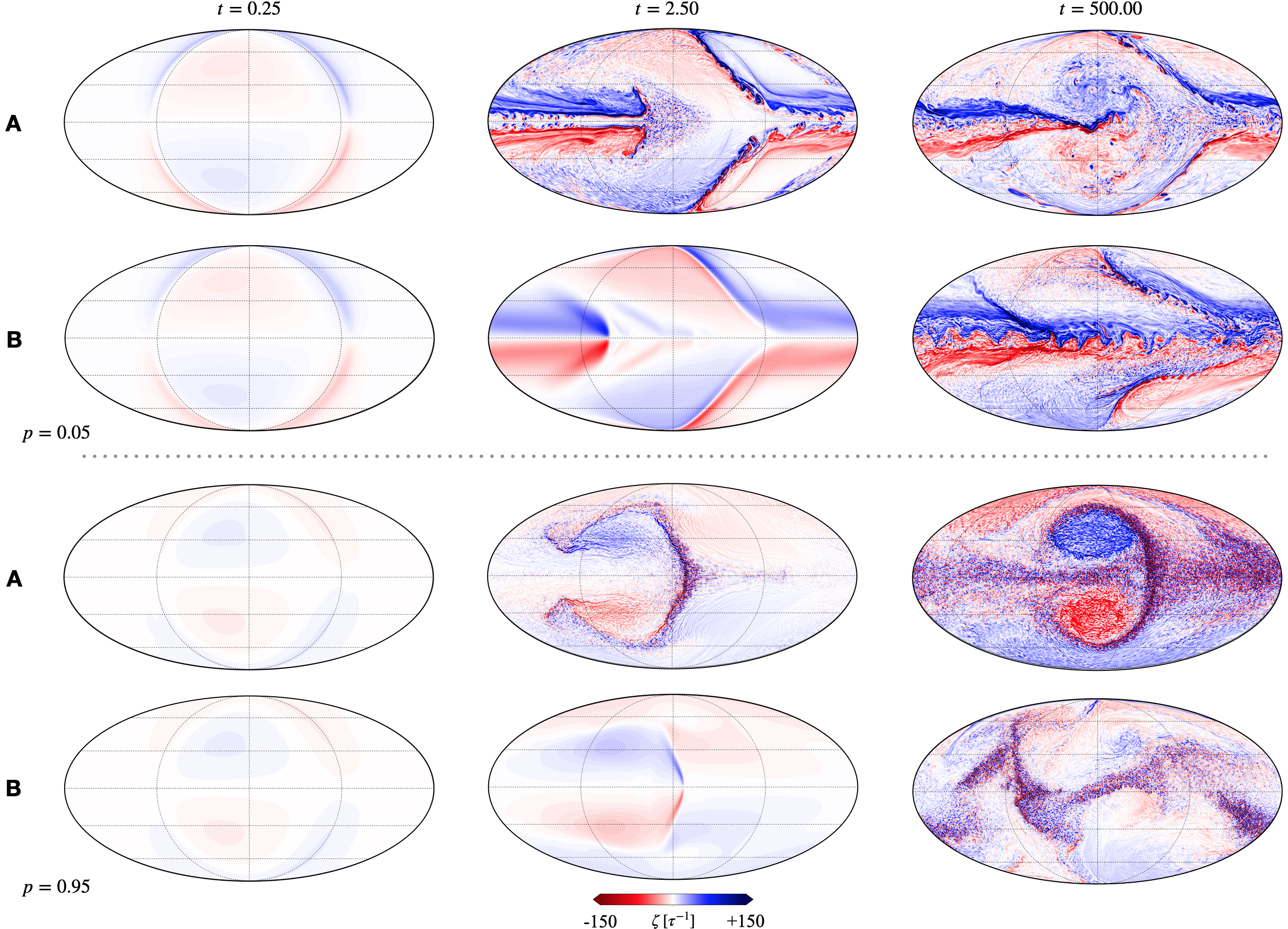
Figure 1: Vorticity field $\zeta$ (in units of $\tau^{-1}$) from two T341L20 resolution simulations (A and B) at two $p$-levels and three times since $t=0$. The fields are in Mollweide projection, centered on the substellar point $(\lambda=0,\,\phi=0)$; here $\lambda$ is the longitude and $\phi$ is the latitude. Simulations (A and B) are identical—except B uses $\mathfrak{p}=1$ (i.e., $\nabla^{2}$) dissipation with coefficient $\nu=5.9\times 10^{-6}$ (in units of $R_{p}^{2}\,\tau^{-1}$), to damp small-scale flow structures more rapidly for $t<3$; both simulations use the same $\mathfrak{p}$ and $\nu$ thereafter. Simulation A is a reference simulation, which uses $\mathfrak{p}=8$ (i.e., $\nabla^{16}$) dissipation with $\nu=1.5\times 10^{-43}$ (in units of $R_{p}^{16}\,\tau^{-1}$), to permit small-scale flow structures to evolve much less encumbered for the entire duration of the simulation ($t=1000$). At $t=0.25$, the fields from the two simulations are essentially identical at both of the $p$-levels. However, at $t=2.5$, the impact of the difference in damping treatment is clear: numerous small-scale vortices along the fronts, jet flanks, and storm peripheries are entirely missing in simulation B. At $t=500$, the two simulations exhibit significant, qualitative differences—long after the difference in dissipation has ceased; note, e.g., the absence of a strong giant modon in B. A brief, “minor” difference at the small scales very early in the simulation has a persistent, major consequence at the large scale.

Fig. 1 presents the main result of this paper. When forced by a large day—night temperature contrast ramped up on a short timescale, energetic small-scale structures quickly emerge in hot-exoplanet atmospheric flows, and the preclusion or mitigation of these structures cause significant differences in the long-term flow and temperature distributions. Here by “short” we mean a period smaller than 1 and by “small” we mean a lateral size smaller than 1/10. The significant role of small-scale structures on the flow has been noted and addressed from the inception of hot-exoplanet atmosphere studies by Cho et al. (2003) and explicitly demonstrated to depend on viscosity and resolution in numerical simulations in subsequent studies (e.g., Thrastarson & Cho, 2011; Cho et al., 2015; Skinner & Cho, 2021; Skinner et al., 2023). In this letter, we highlight the importance of elongated, sharp fronts (that subsequently roll up into long-lived vortices) and internal gravity waves (Watkins & Cho, 2010)—both of which unavoidably arise at the beginning of simulation (as well as throughout the simulation): the structures are generated in response to the atmosphere’s attempt to adjust to the applied forcing.

The figure shows the $\zeta(\lambda,\phi)$ fields from two simulations (A and B) at illustrative $p$-levels (0.05 and 0.95) and times (0.25, 2.50 and 500). The fields are shown in the Mollweide projection, centered at the planet’s substellar point ($\lambda\!=\!0$, $\phi\!=\!0$). The two simulations are identical in every way—except energy is removed more rapidly in a slightly wider range of small scales in simulation B than in simulation A for a very brief interval of time, $t=[0,3)$. Two $p$-levels (corresponding to near the top and near the bottom of the simulation) are presented, but the points made in this paper are generic to the entire range of $p$-levels in the simulation.

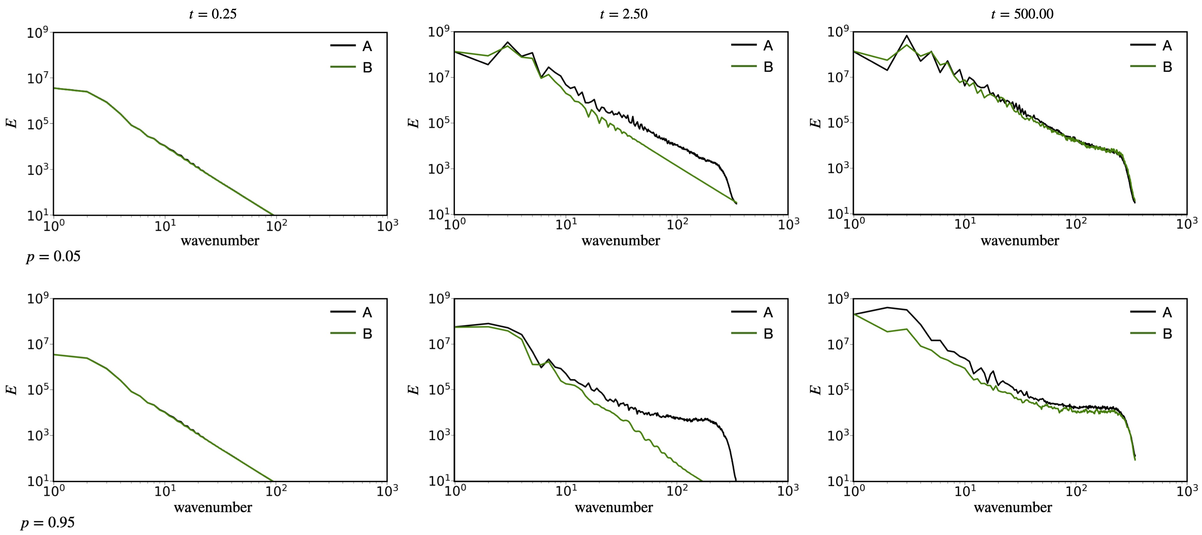
Figure 2: Specific kinetic energy spectrum, $E=E(n)$, of the flows from simulations A and B in Fig. 1 at $p=0.05$ (top row) and $p=0.95$ (bottom row). At $t=0.25$, the spectra are identical for the two simulations at both $p$-levels. At $t=2.5$, the spectra at both $p$-levels are markedly different, especially at large $n$, where the spectra for simulation B are much steeper than those for simulation A. This reflects the absence of small-scale vortices along the fronts, jet flanks and vortex peripheries, in simulation B. At $t=500$, long after all the parameters in both simulations have been rendered identical (at $t=3$), the spectra at both $p$-levels are still very different—particularly at $p=0.95$; notice the very large deficit of $E$ at small $n$. This is due to the absence of a strong giant modon in simulation B. The initial difference in the small scales has spread to the large scales, due to the nonlinearity intrinsic in the solved equations.

At $t=0.25$, the flows of the two simulations are essentially identical (cf., A and B in the left column at both $p$-levels). At this time, the added dissipation in B has not had a chance to act on the flow (as quantified below). However, at $t=2.5$, the difference in dissipation is clearly felt by the flow: sharp vorticity fronts (shear layers) in the eastern hemisphere of the day-side and near the equator are markedly different (cf., A and B in the center column at both $p$-levels). In general, sharp fronts demarcate the outer boundaries of planetary-scale hetons and flanks of an azonal “equatorial jet”; however, unlike in B, the fronts have spawned a large number of small-scale vortices (storms) in A. At $t=500$, long after the simulations have been brought back to an identical dissipation condition, not only are the flows still different but even more so, compared with those at $t=2.5$: hetons are no longer present, and the cyclonic modon clearly seen at the center of the frames in A has grown more intense, while a modon is not really present in B. Note that the difference in the flow is not due to a temporary “phase offset”. The difference persists over the entire duration of the simulations after $t=3$. We emphasize here that this difference cannot be captured below T341 resolution because the structures themselves are not captured (Skinner & Cho, 2021).

Fig. 2 shows the (specific) kinetic energy spectrum, $E=E(n)$, of the flows presented in Fig. 1. In Fig. 2, uniform ranges of $E$ and $n$ are used for ease of comparison. The top row contains the spectra of the flow from the $p=0.05$ level, and the bottom row contains the spectra of the flow from the $p=0.95$ level. In sum, the figure shows that the difference in viscosity, which is limited to the small scales and for only a brief period at the beginning of the simulation, spreads and persists in spectral space—long after the difference has ceased. The spreading is a fundamental property of nonlinearity in equation (1) and also occurs in the full Navier–Stokes equations (e.g., Dobbs-Dixon & Lin, 2008; Mayne et al., 2014; Mendonça et al., 2016), from which equations (1) derive.

At $t=0.25$, the spectra for A and B are identical at both $p$-levels, as expected from the corresponding physical space fields in Fig. 1. Clearly, the dynamics is not affected by the difference in viscosity at this time—at all scales. In contrast, at $t=2.5$, a large difference can be seen between the spectra for A and B—especially at the small scales, $n\gtrsim 20$. In fact, the difference is huge in the $25\lesssim n\lesssim 300$ subrange. At this time all four spectra are still evolving, but the overall shapes of each one are effectively stationary after $t\approx 20$. Long after the dissipation rate has been rendered identical across the entire spectrum (at $t=3$), the spectra at $t=500$ are still noticeably different—this time much more at the large scales, $n\lesssim 20$. At $p=0.05$, the difference is significant for only select $n$’s (e.g., $n=2$ and $n=3$); but, at $p=0.95$, the difference is significant for the entire $n\lesssim 20$ subrange. At the latter $p$-level, the difference is in fact significant across essentially the entire range of well-resolved scales above the dissipation range (i.e., $n\lesssim 200$); this is again consistent with the corresponding physical space fields in Fig. 1.

Broadly, energy is accumulated in both the large-$n$ and small-$n$ subranges (heuristically, $n\gtrsim 100$ and $n\lesssim 10$, respectively). However, the accumulations are different in the two simulations. As the simulations evolve, their spectra become increasingly dissimilar for $n\lesssim 10$, until each simulation reach a different quasi-equilibrium state (Cho et al., 2021). Note that these are the scales which are directly comparable with observations as well as explicitly represented in most current numerical models. Of course, because of the nonlinear interaction, inclusion of $n\gg 10$ is necessary to accurately represent $n\lesssim 10$ (e.g., Boyd, 1989; Skinner & Cho, 2021). Therefore, given the general behavior seen here, it is not difficult to argue that the difference would only increase with resolutions greater than that employed in the present study. It also explains in part why past hot-exoplanet simulations in which small scales have been poorly resolved, or altogether missing, would not be able to produce the result of high-resolution simulations at the large scales—as pointed out in many studies in the past (e.g., Thrastarson & Cho, 2011; Polichtchouk & Cho, 2012; Cho et al., 2015; Skinner & Cho, 2021). Because under-resolved and/or over-dissipated models would not be able to capture the sensitivity and complexity of the flow, they would give a specious appearance of stability or consistency in their predictions for the large scale.

Fig. 3 presents a clearer picture of the behavior over time, focusing on averaged quantities. As already alluded to, these averaged quantities are important for observations. In the figure, the blackbody temperature flux, $\mathscr{F}(t)\equiv\sigma\langle T^{\,4}\rangle_{\,\mbox{\tiny SS}}$, is considered; here $\langle\,(\,\cdot\,)\,\rangle_{\,\mbox{\tiny SS}}$ represents a line-of-sight projection (a cosine factor) weighted average over a disk centered on the substellar point (SS), and $\sigma$ is the Stefan–Boltzmann constant. The flux for each simulation is normalized by the initial flux, $\tilde{\mathscr{F}}_{0(\cdot)}\equiv\langle\,T_{0(\cdot)}^{\,4}\rangle_{\,\mbox{\tiny SS}}$, so that $\tilde{\mathscr{F}}_{(\cdot)}=\tilde{\mathscr{F}}_{(\cdot)}\,/\,\tilde{\mathscr{F}}_{0(\cdot)}$; for example, $\tilde{\mathscr{F}}_{\mbox{\tiny A}}=\tilde{\mathscr{F}}_{\mbox{\tiny A}}(t)$ is the normalized flux for simulation A. The value of the normalization is same for both simulations and is also independent of the location of the disk center, due to the spatially uniform temperature distribution used at $t=0$. The duration, $t=[0,500]$, is shown in the figure, but the general behavior is unchanged up to $t=1000$. We note that such a long duration is unlikely to be physically realistic, given the highly idealized initial and forcing conditions employed; however, it does illustrate the robustness of the behavior discussed.

As can be seen, large differences in $\mathscr{F}(t)$ persist (even when the field is averaged over a disk) over a long time. The difference ranges approximately $\pm\,0.4$ at $p=0.05$ and $\pm\,0.1$ at $p=0.95$ for $t\gtrsim 8$ and continues for the entire duration of the simulations. The variations correspond to disk-averaged temperature differences of up to $\pm\,100$ K at $p=0.05$ and $\pm\,75$ K at $p=0.95$. Such differences, which stem from the acute sensitivity inherent in the equations, directly impact the ability to correctly predict and/or interpret observations from current and next-generation telescopes (e.g., James Webb Space Telescope and Ariel). This underscores the critical importance of accurately and consistently representing small-scale flows throughout the entirety of the simulation. The absence of such representation, even for a brief period, permanently degrades the fidelity of the model predictions.

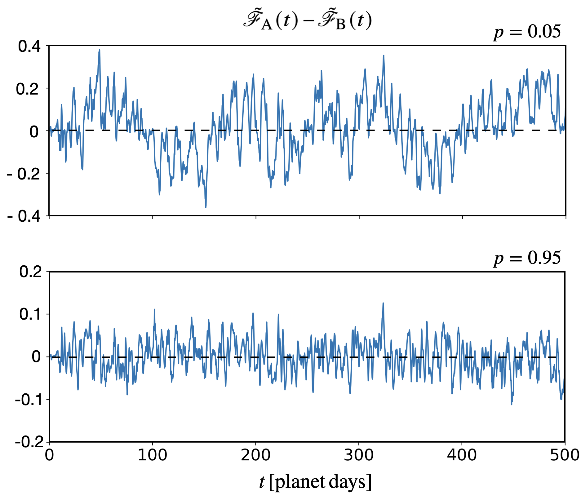
Figure 3: Disk-averaged, normalized, blackbody-temperature flux $\tilde{\mathscr{F}}(t)$ difference between simulations A and B in Fig. 1 at the indicated $p$-levels. The flux is averaged over a disk centered on the substellar point, $(\lambda\!=\!0,\,\phi\!=\!0)$ and weighted by a cosine projection factor (see text). Even under averaging, a significant difference is present—with the difference increasing towards the top of the simulation domain. Here the maximum deviation from the mean corresponds to an averaged temperature ($\langle\,T\rangle_{\mbox{\tiny SS}}$) difference of $\approx\!100$ K and $\approx\!75$ K at $p=0.05$ and $p=0.95$ (i.e., $\approx\!11.5\%$ and $\approx\!5\%$ of the planet’s disk-averaged $T$ at secondary eclipse, respectively). The differences are chaotic in time and is not due to a simple “phase-shift” between the flows in the two simulations. Only up to $t=500$ is shown for clarity, but the behavior is qualitatively the same up to $t=1000$, the duration of these simulations. Significantly, the differences are large enough to affect the interpretations of current- and next-generation telescope observations.

Fig. 4 shows a more detailed picture of the effect of the differences under “well resolved” condition. The figure presents $\tilde{\mathscr{F}}(t)$ at $p=0.95$ for six T341L20 simulations—all identical except for the $(\nu,\,\mathfrak{p})$ pairs, $(1.5\times 10^{-43},\,8)$ and $(5.9\times 10^{-6},\,1)$; see Eq. 2. In the simulations, the dissipation applied is “switched on or off” at different times, indicated by a background shading of green and red for $\nabla^{16}$ and $\nabla^{2}$ operators, respectively; the dashed lines indicate the time the dissipation changes during the simulation. In the figure, panels A and D present reference simulations, with a fixed dissipation setting for all $t$. Panels B and C present simulations with parameters identical to those in the simulation of A but with a stronger dissipation rate, $(\nu,\,\mathfrak{p})=(5.9\times 10^{-6},\,1)$, applied for $t<3$ and $t<20$ respectively. Panels E and F present simulations with parameters identical to those in the simulation of D but with a weaker dissipation rate, $(\nu,\,\mathfrak{p})=(1.5\times 10^{-43},\,8)$, also applied for $t<3$ and $t<20$ respectively.

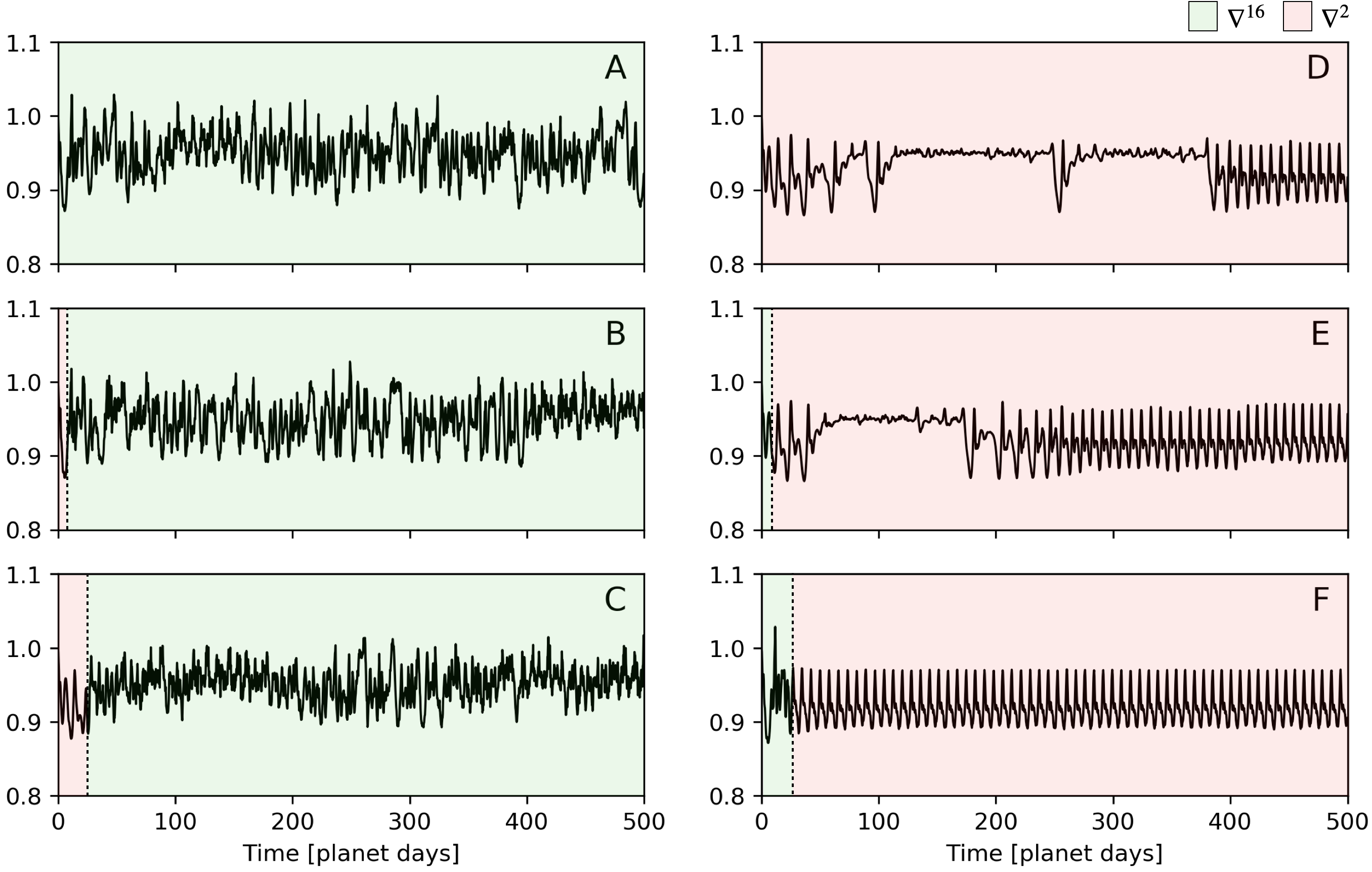
Figure 4: Time-series of $\tilde{\mathscr{F}}(t)$ at $p=0.95$ for six simulations (A–F), in which the duration and value of $(\mathfrak{p},\nu)$ pairs, $(8,1.5\times 10^{-43})$ and $(1,5.9\times 10^{-6})$, are different. The $\mathfrak{p}$ values, corresponding to $\nabla^{16}$ and $\nabla^{2}$ operators, are distinguished by the background shading (light green and light red, respectively), and the time at which the dissipation form changes during the simulation is indicated by the dashed line. Otherwise, all simulations are identical—including the values of normalization and $\tilde{\mathscr{F}(0)}$ ($=\!1$). The simulation in A is the simulation in Fig. 1A. (A, D) are reference simulations, with $\mathfrak{p}$ and $\nu$ fixed for the entire duration. (B, C) correspond to simulations that are identical to A, but with enhanced dissipation of small scales for $t<3$ and $t<20$, respectively. (E, F) correspond to simulations that are identical to D, but with reduced dissipation of small scales for $t<3$ and $t<20$, respectively. Having the reduced dissipation on for a longer period appears to hasten the transition to a large-amplitude oscillatory state (cf., D, E and F); and, having the enhanced dissipation on for a longer period appears to introduce long-period variation (cf., B and C). Differences in dissipation rate of small scales influence the evolution in complicated ways.

Broadly, two distinct types of $\tilde{\mathscr{F}}(t)$ behaviors emerge (cf., Skinner & Cho, 2021): 1) a dynamic and chaotic large-scale flow characterized by multiple, persistent large-amplitude oscillations; and, 2) persistent, regular oscillations that “kick in” after a period of small-amplitude oscillations. The two types can be seen in the left and right columns of Fig. 4, respectively. The first type is caused by dynamical instability and turbulent motion of energetic, planetary-scale vortices, which ultimately migrate around the planet; these giant vortices, which may be singlets or doublets (Skinner et al., 2023), interact with a large number of small vortices during the migration in a way reminiscent of Brownian motion (panels A–C). In this case, the planet’s vorticity and temperature fields are highly inhomogeneous, with strong meridional (north–south) asymmetries and vigorous mixing on the large scale. The second type is caused by a long-lived, planetary-scale, meridionally symmetric modon, which is weaker (lower $|\zeta|$) than the giant vortices in the first type. After a transient period of large excursions from near the substellar point at the beginning of the simulation, there is generally a period of “quiescence”, when the modon’s position is nearly fixed at the substellar point (e.g., $120\lesssim t\lesssim 260$ in panel D). After this quiescent state, the modon transitions to a one of westward “migration” around the planet—subsequently either transitioning back to the quiescent state ($t\approx 275$ in panel D) or remaining in the migrating state ($t\approx 230$ in panel D).

Notice that the quiescent state is not always present in a simulation (panel F). However, when it is present (panels D and E), there is nearly a fourfold reduction in $\tilde{\mathscr{F}}$ variations as well as a sustained high amplitude in $\tilde{\mathscr{F}}$ compared with $\tilde{\mathscr{F}}$ in the migrating state (present in all of panels D–F). Both the reduction of variation and sustenance of high amplitude occur because there is little or no heat transport away from the dayside. In contrast, when the modon migrates westward, it mixes and advects heat to the western terminator or beyond. The timescale of the mixing/advection is fast, evinced by the short decay time of the regular peaks seen in panels D–F; it is equal to the radiative cooling timescale for the $p$-level shown in the figure.

It is clear from Fig. 4 that model predictions are highly sensitive to the dissipation rate of the small scales. It follows that the sensitivity would also be exhibited when the small scales are entirely absent. For example, simulations in the right column of the figure suppress the small scales throughout the majority of their evolution, but permit small scales to be less encumbered for the first 3 and 20 days (E and F, respectively). The resulting evolutions are noticeably different in the two simulations, despite their being identical otherwise. Less dramatic, but still noticeable, behaviors are seen in the opposite situation, in which the small scales are more suppressed for the first 3 and 20 days of the evolution (B and C, respectively). In C, a long-period variation not seen in A appears in the evolution; in B, a suggestive transition to a “quiescent”-like state is observed (cf., A). Even a difference for a very brief period, early in the evolution (e.g., $t<3$), could lead to an observationally significant variation later in the evolution, stemming from the inherent nature of nonlinearity.

4 Discussion

In this letter, we have presented results from high-resolution atmospheric flow simulations with a setup (initial, boundary and forcing conditions) commonly employed for hot-exoplanets. Our simulations explicitly show that the behavior of the atmosphere at the large-scale is highly sensitive to the rate of energy loss in the small scales (both intentional and not). Surprisingly, the sensitivity is present even if the increase in the rate is operating only for a very brief period. Hence, deviation from high-resolution results are fully expected when the small scales are poorly resolved or altogether missing, as demonstrated by Skinner & Cho (2021); as in that study, the sensitivity is comprehensively illustrated in physical, spectral and temporal spaces here. In this study, we clearly demonstrate that high-resolution is necessary for generating accurate predictions—especially for comparison with, and interpretation of, observations.

More broadly, high-resolution is also critical for understanding ageostrophic, turbulent flows in general. The presence (or preclusion) of the small-scale structures, which appear almost immediately in the flow ($t\lesssim 1$), leads the atmospheres to settle into a qualitatively different quasi-equilibrium state. The small-scale flow structures generated at early times of the evolution are sharp, elongated fronts that roll up into energetic vortices and radiated gravity waves. These form in response to the atmosphere’s attempt to adjust to the applied forcing—regardless of the degree to which the radiative process has been idealized: the aggressive response is due to the rapidity of the thermal relaxation to a high day–night temperature gradient. The need for high resolution and balancing to address such atmospheres has been noted since the beginning of exoplanet atmospheric dynamics studies by Cho et al. (2003): in that study, nonlinear balancing and slow lead-up to the full thermal forcing have been employed at T341 resolution.

This work has significant implications for general circulation and climate modeling of hot-exoplanets. Models that use any combination of low order dissipation, low spatial or temporal resolution, high explicit viscosity coefficients, and/or strong basal drags to force numerical stabilization are at risk. This is because all of these expediencies preclude small-scale flows from being adequately captured throughout the simulation’s evolution. In our view, it is unlikely that the state of the hot-exoplanet atmosphere can be usefully captured in such models.

Accurately simulating the atmosphere is a complex and difficult problem. This is the case even for the Earth, for which observation-infused inputs to the numerical models are available and the dynamics are geostrophically balanced. Importantly, effects of small-scales very similar to those described here are well known in Earth climate simulation studies (Rial et al., 2004; Sriver et al., 2015; Deser et al., 2020); however, as expected, their effects are weaker compared to those for hot-exoplanets. Despite this, the effects have not been much explored in exoplanet studies. The preclusion of small-scale structures poses a particularly critical problem in hot-exoplanets. The high sensitivity of the overall flow to small-scale structures, which arise early in the simulation, means that considerable care must be taken to: 1) sensibly initialize the simulation; and, 2) accurately represent structures of wide-ranging scales throughout the entire duration of the simulation.

5 Acknowledgments

The authors thank Joonas Nättilä and Quentin Changeat for helpful discussions. JWS is supported by NASA grant 80NSSC23K0345 and a Simons Foundation Pivot Fellowship. JWS is grateful for the hospitality of the Center for Computational Astrophysics, Flatiron Institute, where some of this work was completed. JYKC performed part of this work at the Aspen Center for Physics, which is supported by National Science Foundation grant PHY-2210452. This work used high performance computing at the San Diego Super Computing Centre through allocation PHY-230189 from the Advanced Cyberinfrastructure Coordination Ecosystem: Services & Support (ACCESS) program, which is supported by National Science Foundation grants #2138259, #2138286, #2138307, #2137603, and #2138296. This work also used high-performance computing awarded by the Google Cloud Research Credits program GCP19980904.

References

- Asselin (1972) Asselin, R. 1972, Monthly Weather Review, 100, 487, doi: 10.1175/1520-0493(1972)100<0487:FFFTI>2.3.CO;2
- Boyd (1989) Boyd, J. P. 1989, Chebyshev & Fourier Spectral Methods (Berlin, Heidelberg: Springer Berlin Heidelberg)
- Cho et al. (2003) Cho, J. Y-K., Menou, K., Hansen, B. M. S., & Seager, S. 2003, The Astrophysical Journal Letters, 587, 117, doi: 10.1086/375016
- Cho et al. (2008) —. 2008, The Astrophysical Journal, 675, 817, doi: 10.1086/524718
- Cho et al. (2015) Cho, J. Y-K., Polichtchouk, I., & Thrastarson, H. Th. 2015, Monthly Notices of the Royal Astronomical Society, 454, 3423, doi: 10.1093/mnras/stv1947
- Cho et al. (2021) Cho, J. Y-K., Skinner, J. W., & Thrastarson, H. Th. 2021, The Astrophysical Journal Letters, 913, 832, doi: 10.3847/2041-8213/abfd37
- Cooper & Showman (2006) Cooper, C. S., & Showman, A. P. 2006, The Astrophysical Journal, 649, 1048, doi: 10.1086/506312
- Deser et al. (2020) Deser, C., Lehner, F., Rodgers, K. B., et al. 2020, Nature Climate Change, 10, 277, doi: 10.1038/s41558-020-0731-2
- Dobbs-Dixon & Lin (2008) Dobbs-Dixon, I., & Lin, D. N. C. 2008, The Astrophysical Journal, 673, 513, doi: 10.1086/523786
- Eliassen (1984) Eliassen, A. 1984, Quarterly Journal of the Royal Meteorological Society, 110, 1, doi: https://doi.org/10.1002/qj.49711046302
- Hammond & Abbot (2022) Hammond, M., & Abbot, D. S. 2022, Monthly Notices of the Royal Astronomical Society, 511, 2313, doi: 10.1093/mnras/stac228
- Hogg & Stommel (1985) Hogg, N. G., & Stommel, H. M. 1985, Proceedings of the Royal Society of London. A. Mathematical and Physical Sciences, 397, doi: 10.1098/rspa.1985.0001
- Kizner (2006) Kizner, Z. 2006, Physics of Fluids, 18, doi: 10.1063/1.2196094
- Lorenz (1963) Lorenz, E. N. 1963, Journal of the Atmospheric Sciences, 20, 130, doi: 10.1175/1520-0469(1963)020<0130:DNF>2.0.CO;2
- Lorenz (1964) —. 1964, Tellus, 16, 1, doi: 10.1111/j.2153-3490.1964.tb00136.x
- Mayne et al. (2014) Mayne, N. J., Baraffe, I., Acreman, D. M., et al. 2014, Astronomy & Astrophysics, 561, doi: 10.1051/0004-6361/201322174
- Mendonça et al. (2016) Mendonça, J. M., Grimm, S. L., Grosheintz, L., & Heng, K. 2016, The Astrophysical Journal, 829, doi: 10.3847/0004-637X/829/2/115
- Menou & Rauscher (2009) Menou, K., & Rauscher, E. 2009, Astrophysical Journal, 700, 887, doi: 10.1088/0004-637X/700/1/887
- Phillips (1963) Phillips, N. A. 1963, Reviews of Geophysics, 1, 123, doi: https://doi.org/10.1029/RG001i002p00123
- Poincaré (1914) Poincaré, H. 1914, Science and Method (South Bend, IN: Dover Publications)
- Polichtchouk & Cho (2012) Polichtchouk, I., & Cho, J. Y-K. 2012, Monthly Notices of the Royal Astronomical Society, 424, 1307, doi: 10.1111/j.1365-2966.2012.21312.x
- Polichtchouk et al. (2014) Polichtchouk, I., Cho, J. Y-K., Watkins, C., et al. 2014, Icarus, 229, 355, doi: 10.1016/j.icarus.2013.11.027
- Rauscher & Menou (2010) Rauscher, E., & Menou, K. 2010, The Astrophysical Journal, 714, 1334, doi: 10.1088/0004-637X/714/2/1334
- Rial et al. (2004) Rial, J. A., Pielke Sr., R. A., Beniston, M., et al. 2004, Climatic Change, 65, 11, doi: 10.1023/B:CLIM.0000037493.89489.3f
- Robert (1966) Robert, A. J. 1966, Journal of the Meteorological Society of Japan. Ser. II, 44, 237, doi: 10.2151/jmsj1965.44.5_237
- Showman et al. (2008) Showman, A. P., Cooper, C. S., Fortney, J. J., & Marley, M. S. 2008, The Astrophysical Journal, 682, 559, doi: 10.1086/589325
- Showman & Guillot (2002) Showman, A. P., & Guillot, T. 2002, Astronomy & Astrophysics, 385, 166, doi: 10.1051/0004-6361:20020101
- Skinner & Cho (2021) Skinner, J. W., & Cho, J. Y-K. 2021, Monthly Notices of the Royal Astronomical Society, 504, 5172, doi: 10.1093/mnras/stab971
- Skinner & Cho (2022) —. 2022, Monthly Notices of the Royal Astronomical Society, 511, 3584, doi: 10.1093/mnras/stab2809
- Skinner et al. (2023) Skinner, J. W., Nättilä, J., & Cho, J. Y-K. 2023, Phys. Rev. Lett., 131, 231201, doi: 10.1103/PhysRevLett.131.231201
- Sriver et al. (2015) Sriver, R. L., Forest, C. E., & Keller, K. 2015, Geophysical Research Letters, 42, 5468, doi: https://doi.org/10.1002/2015GL064546
- Thrastarson & Cho (2010) Thrastarson, H. Th., & Cho, J. Y-K. 2010, The Astrophysical Journal, 716, 144, doi: 10.1088/0004-637X/716/1/144
- Thrastarson & Cho (2011) —. 2011, The Astrophysical Journal, 729, 117, doi: 10.1088/0004-637X/729/2/117
- Watkins & Cho (2010) Watkins, C., & Cho, J. Y-K. 2010, The Astrophysical Journal, 714, doi: 10.1088/0004-637X/714/1/904