Learning Discrete Concepts in Latent Hierarchical Models

Abstract

Learning concepts from natural high-dimensional data (e.g., images) holds potential in building human-aligned and interpretable machine learning models. Despite its encouraging prospect, formalization and theoretical insights into this crucial task are still lacking. In this work, we formalize concepts as discrete latent causal variables that are related via a hierarchical causal model that encodes different abstraction levels of concepts embedded in high-dimensional data (e.g., a dog breed and its eye shapes in natural images). We formulate conditions to facilitate the identification of the proposed causal model, which reveals when learning such concepts from unsupervised data is possible. Our conditions permit complex causal hierarchical structures beyond latent trees and multi-level directed acyclic graphs in prior work and can handle high-dimensional, continuous observed variables, which is well-suited for unstructured data modalities such as images. We substantiate our theoretical claims with synthetic data experiments. Further, we discuss our theory’s implications for understanding the underlying mechanisms of latent diffusion models and provide corresponding empirical evidence for our theoretical insights.

1 Introduction

Learning semantic discrete concepts from unstructured high-dimensional data, such as images and text, is crucial to building machine learning models with interpretability, transferability, and compositionality, as empirically demonstrated by extensive existing work [1, 2, 3, 4, 5, 6, 7, 8, 9, 10, 11]. Despite these empirical successes, limited work is devoted to the theoretical front: the notions of concepts and their relations are often heuristically defined. For example, concept bottleneck models [12, 13] use human-specified annotations and recent methods [14, 15, 16] employ pretrained multimodal models like CLIP [17] to explain features with neural language. This lack of rigorous characterization impedes a deeper understanding of this task and the development of principled learning algorithms.

In natural images, the degree/extent of certain attributes (e.g., position, lighting) is often presented in a continuous form and main concepts of practical concern are often discrete in nature (e.g., object classes and shapes). Moreover, these concepts are often statistically dependent, with the dependence potentially resulting from some higher-level concepts. For example, the correlation of a specific dog’s eye features and fur features may arise from a high-level concept for breeds (Figure 1). Similarly, even higher-level concepts may exist and induce dependence between high-level concepts, giving rise to a hierarchical model that characterizes all discrete concepts at different abstraction levels underlying high-dimensional data distributions. In this work, we focus on concepts that can be defined as discrete latent variables and related via a hierarchical model. Under this formalization, the query on the recoverability of concepts and their relations from unstructured high-dimensional distribution (e.g., images) amounts to the following causal identification problem:

Under what conditions is the discrete latent hierarchical causal model identifiable from high-dimensional continuous data distributions?

Identification theory for latent hierarchical causal models has been a topic of sustained interest. Recent work [18, 19, 20] investigates identification conditions of latent hierarchical structures under the assumption that the latent variables are continuous and influence each other through linear functions. The linearity assumption fails to handle the general nonlinear influences among discrete variables. Another line of work focuses on discrete latent models. Pearl [21], Choi et al. [22] study latent trees with discrete observed variables. The tree structure can be over-simplified to capture the complex interactions among concepts from distinct abstract levels (e.g., multiple high-level concepts can jointly influence a lower-level one). Gu and Dunson [23] assume that binary latent variables can be exactly grouped into levels and causal edges often appear between adjacent levels, which can also be restrictive. Moreover, these papers assume observed variables are discrete, falling short of modeling the continuous distribution like images as the observed variables. Similar to our goal, Kivva et al. [24] show the discrete latent variables adjacent to the potentially continuous observed variables can be identified. However, their theory assumes the absence of higher-level latent variables and thus cannot handle latent hierarchical structures. More related work can be found in Appendix A1.

In this work, we show identification guarantees for the discrete hierarchical model under mild conditions on the generating function and causal structures. Specifically, we first show that when continuous observed variables (i.e., the leaves of the hierarchy) preserve the information of their adjacent discrete latent variables (i.e., direct parents in the graph), we can extract the discrete information from the continuous observations and further identify each discrete variable up to permutation indeterminacy. Given these “low-level” discrete latent variables, we establish graphical conditions to identify the discrete hierarchical model that fully explains the statistical dependence among the identified “low-level” discrete latent variables. Our conditions permit multiple paths within latent variable pairs and flexible locations of latent variables , encompassing a large family of graph structures including as special cases non-hierarchical structures [24], trees [21, 22, 25, 26] and multi-level directed acyclic graphs (DAGs) [23, 27] (see example graphs in Figure 2). Taken together, our work establishes theoretical results for identifying the discrete latent hierarchical model governing high-dimensional continuous observed variables, which to the best of our knowledge is the first effort in this direction. We corroborate our theoretical results with synthetic data experiments.

As a implication of our theorems, we discuss a novel interpretation of the state-of-the-art latent diffusion (LD) models [28] through the lens of a hierarchical concept model. We interpret the denoising objective at different noise levels as estimating latent concept embeddings at corresponding hierarchical levels in the causal model, where a higher noise level corresponds to high-level concepts. This perspective explains and unifies these seemingly orthogonal threads of empirical insights and gives rise to insights for potential empirical improvements. We deduce several insights from our theoretical results and verify them empirically. In summary, our main contributions are as follows.

• We formalize the framework of learning concepts from high-dimensional data as a latent-variable identification problem, capturing concepts at different abstraction levels and their interactions.

• We present identification theories for the discrete latent hierarchical model. To the best of our knowledge, our result is the first to address discrete latent hierarchical model beyond trees [21, 26] and multi-level DAGs [23] while capable of handling high-dimensional observed variables.

• We provide an interpretation of latent diffusion models as hierarchical concept learners. We supply empirical results to illustrate our interpretation and showcase its potential benefits in practice.

2 Discrete Hierarchical Models

Data-generating process.

We formulate the data-generating process as the following latent-variable model. Let $\mathbf{x}$ denote the continuous observed variables $\mathbf{x}:=[x_{1},\cdots,x_{n}]\in\mathcal{X}\subset\mathbb{R}^{d_{\mathbf{x}}}$ which represents the high-dimension data we work with in practice (e.g., images). Let $\mathbf{d}:=[d_{1},\cdots,d_{n_{d}}]$ be discrete latent variables that are direct parents to $\mathbf{x}$ (as shown in Figure 1(b)) and take on values from finite sets, i.e., $d_{i}\in\Omega_{i}^{(d)}$ for all $i\in[d_{i}]$ and $2\leq\left\lvert\Omega_{i}^{(d)}\right\rvert<\infty$. We denote the joint domain as $\Omega^{(d)}:=\Omega_{1}^{(d)}\times\cdots\times\Omega_{n_{d}}^{(d)}$. These discrete variables are potentially related to each other causally (e.g., $d_{4}$ and $d_{5}$ in Figure 1(c)) or via higher-level latent variables (e.g., $d_{1}$ and $d_{2}$ in Figure 1(c)). Let $\mathbf{c}:=[c_{1},\cdots,c_{n_{c}}]\in\mathcal{C}\subset\mathbb{R}^{d_{c}}$ be continuous latent variables that represent the continuous information conveyed in observed variables $\mathbf{x}$. The generating process is defined in Equation 1 and illustrated in Figure 1(a).

$$\mathbf{x}:=g(\mathbf{d},\mathbf{c}),$$ (1)

where we denote the generating function with $g:[\mathbf{d},\mathbf{c}]\mapsto\mathbf{x}$. We denote the resultant bipartite graph from $[\mathbf{d},\mathbf{c}]$ to $\mathbf{x}$ as $\Gamma$. In this context of image generation, the discrete subspace $\mathbf{d}$ gives a description of concepts present in the image $\mathbf{x}$ (e.g., a dog’s appearance, background objects), and the continuous subspace $\mathbf{c}$ controls extents/degrees of specific attributes (e.g., sizes, lighting, and angles).

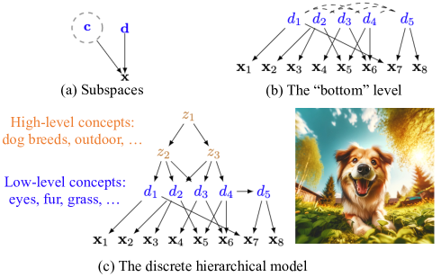
Figure 1: Latent causal models. The dashed circle in (a) indicates that the continuous variable $\mathbf{c}$ can be viewed as an exogenous variable. Dashed edges in (b) indicate potential statistical dependence.

Discrete hierarchical models.

As discussed above, discrete variables $d_{1},\dots,d_{n_{d}}$ represent distinct concepts that may be dependent either causally or purely statistically via higher-level concepts, as visualized in Figure 1(c). For instance, the dog’s eye features and nose features are dependent, which a higher-level concept “breeds” could explain. We denote such higher-level latent discrete variables as $\mathbf{z}:=[z_{1},\cdots,z_{n_{z}}]$, where $z_{i}\in\Omega_{i}^{(z)}$ for all $i\in[z_{i}]$ and $2\leq\left\lvert\Omega_{i}^{(z)}\right\rvert<\infty$ and $\Omega^{(z)}:=\Omega_{1}^{(z)}\times\cdots\times\Omega_{n_{z}}^{(z)}$. Graphically, these variables $\mathbf{z}$ are not directly adjacent to observed variables $\mathbf{x}$ (Figure 1(c)). High-level discrete variables $\mathbf{z}$ may constitute a hierarchical structure until the dependence in the system is fully explained. Since the discrete variables encode major semantic concepts in the data, this work primarily concerns discrete variables $\mathbf{d}$ and its underlying causal structure. The continuous subspace $\mathbf{c}$ can be viewed as exogenous variables and is often omitted in the causal graph (e.g., Figure 1(b)). We leave identifying continuous attributes in $\mathbf{c}$ as future work.

Given this, we define the discrete hierarchical model as follows. The discrete hierarchical model (Figure 1(c)) $\mathcal{G}:=(\mathbf{E},\mathbf{V})$ is a DAG that comprises discrete latent variables $d_{1},\cdots,d_{n_{d}},z_{1},\cdots,z_{n_{z}}$. We denote that directed edge set with $\mathbf{E}$ and the collection of all variables with $\mathbf{V}:=\{\mathbf{D},\mathbf{Z}\}$, where $\mathbf{D}$ and $\mathbf{Z}$ are vectors $\mathbf{d}$ and $\mathbf{z}$ in a set form and all leaf variables in $\mathcal{G}$ belong to $\mathbf{D}$. We assume the distribution over all variables $\mathbf{V}$ respects the Markov property with respect to the graph $\mathcal{G}$. We denote all parents and children of a variable with $\text{Ch}(\cdot)$ and $\text{Pa}(\cdot)$ respectively. If a set of variables $\mathbf{A}\subset\mathbf{V}$ has no other parents than $\mathbf{B}$, we say $\mathbf{A}$ is the pure children of $\mathbf{B}$ (Definition A8), i.e., $\mathbf{A}=\text{PCh}_{\mathcal{G}}(\mathbf{B})$. As shown in Figure 1(c), $x_{1}$ is a pure child of $d_{1}$.

Objectives.

Formally, given only the observed distribution $p(\mathbf{x})$, we aim to:

1. identify discrete variables $\mathbf{d}$ and the bipartite graph $\Gamma$;

2. identify the hierarchical causal structure $\mathcal{G}$.

3 Identification of Discrete Latent Hierarchical Models

We present our theoretical results on the identifiability of discrete latent variables $\mathbf{d}$ and the bipartite graph $\Gamma$ in Section 3.2 (i.e., Objective 1) and the hierarchical model $\mathcal{G}$ in Section 3.3 (i.e., Objective 2).

Additional notations.

We denote the set containing components of $\mathbf{x}$ with $\mathbf{X}$, the set of all variables with $\mathbf{V}^{*}:=\mathbf{V}\cup\mathbf{X}$, the entire edge set with $\mathbf{E}^{*}:=\mathbf{E}\cup\Gamma$, and the entire causal model with $\mathcal{G}^{*}:=(\mathbf{V}^{*},\mathbf{E}^{*})$. As the true generating process involves $\mathbf{d}$, $\mathbf{c}$, $g$, $\Gamma$, and $\mathcal{G}$ (defined in Section 2), we define their statistical estimates with $\hat{\mathbf{d}}$, $\hat{\mathbf{c}}$, $\hat{g}$, and $\hat{\Gamma}$ through maximum likelihood estimation over the observed distribution $p(\mathbf{x})$ while respecting conditions on the true generating process.

3.1 General Conditions for Discrete Latent Models

It is well known that causal structures cannot be identified without proper assumptions. For instance, one may merge two adjacent discrete variables $d_{1}\in\Omega^{(d)}_{1}$ and $d_{2}\in\Omega^{(d)}_{2}$ into a single variable $\tilde{d}\in\Omega^{(d)}_{1}\times\Omega^{(d)}_{2}$ while preserving the observed distribution $p(\mathbf{x})$. We introduce the following basic conditions on the discrete latent model to eliminate such ill-posed situations.

Condition 3.1 (General Latent Model Conditions).

1. [Non-degeneracy]: ${\mathbb{P}}\left(\mathbf{d}=k_{1},\mathbf{z}=k_{2}\right)>0$, for all $(k_{1},k_{2})\in\Omega^{(d)}\times\Omega^{(z)}$; for all variable $v\in\mathbf{V}^{*}$, ${\mathbb{P}}\left(v|\text{Pa}(v)=k_{1}\right)\neq{\mathbb{P}}\left(v|\text{Pa}(v)=k_{2}\right)$ if $k_{1}\neq k_{2}$.

2. [No-twins]: Distinct latent variables have distinct neighbors $\text{ne}(V_{1})\neq\text{ne}(v_{2})$, if $v_{i}\neq v_{j}\in\mathbf{V}$.

3. [Maximality]: There is no DAG $\tilde{\mathcal{G}}^{*}:=(\tilde{\mathbf{V}}^{*},\tilde{\mathbf{E}}^{*})$ resulting from splitting a latent variable in $\mathcal{G}^{*}$, such that ${\mathbb{P}}\left(\tilde{\mathbf{V}}^{*}\right)$ is Markov w.r.t. $\tilde{\mathcal{G}}^{*}$ and $\tilde{\mathcal{G}}^{*}$ satisfies ii.

Discussion.

Condition 3.1 is a necessary set of conditions for identifying latent discrete models, which is employed and discussed extensively [24, 29]. Intuitively, Condition 3.1-i excludes dummy discrete states and graph edges that exert no influence on the observed variables $\mathbf{x}$. Condition 3.1-ii,iii constrain the latent model to be the most informative graph without introducing redundant latent variables, thus forbidding arbitrary merging and splitting over latent variables.

3.2 Discrete Component Identification

We show with access to only the observed data $\mathbf{x}$, we can identify each discrete component $d_{i}$ up to permutation indeterminacy (Definition 3.2) and a corresponding bipartite graph equivalent to $\Gamma$.

Definition 3.2 (Component-wise Identifiability).

Variables $\mathbf{d}\in\mathbb{N}^{n_{d}}$ and $\hat{\mathbf{d}}\in\mathbb{N}^{n_{d}}$ are identified component-wise if there exists a permutation $\pi$, such that $\hat{d}_{i}=h_{i}(d_{\pi(i)})$ with invertible function $h_{i}$.

That is, our estimation $\hat{d}_{i}$ captures full information of $d_{\pi(i)}$ and no information from $d_{j}$ such that $j\neq\pi(i)$. The permutation is a fundamental indeterminacy for disentanglement [30, 31, 32, 24].

Remarks on the problem.

A large body of prior work [30, 33, 34] requires continuous or even differentiable density function over all latent variables and domain/class labels or counterfactual counterparts to generate variation. Thus, their techniques do not transfer naturally to our latent space with both continuous and discrete parts $[\mathbf{c},\mathbf{d}]$ and no supervision of any form. With a similar goal, Kivva et al. [24] assumes access to an oracle (Definition A1) to the mixture distribution over $p(\mathbf{x})$, which is not directly available in the general case here. Kivva et al. [29] assumes a specific parametric generating process, whereas we focus on a generic non-parametric generative model (Equation 1).

High-level description of our proposed approach.

We decompose the problem into two tractable subproblems: 1) extracting the global discrete state $\mathbf{d}$ from the mixing with the continuous variable $\mathbf{c}$; 2) further identifying each discrete component $d_{i}$ from the mixing with other discrete components $d_{j}$ ($i\neq j$) and the causal graph $\Gamma$. For 1), we show that, perhaps surprisingly, minimal conditions on the generating function $g$ suffice to remove the information of $\mathbf{c}$ and thus identify the global state of $\mathbf{d}$. For 2), we observe that the identification results in 1) can be viewed as a mixture oracle over $p(\mathbf{x})$, which enables us to employ techniques from Kivva et al. [24] to solve the problem.

We introduce key conditions and formal theoretical statements as follows.

Condition 3.3 (Discrete Components Identification).

1. [Open & Connected Spaces] The continuous support $\mathcal{C}\subset\mathbb{R}^{n_{c}}$ is open and connected.

2. [Invertibility & Continuity]: The generating function $g$ in equation 1 is invertible, and for any fixed $\mathbf{d}$, $g(\mathbf{d},\cdot)$ and its inverse are continuous.

3. [Non-Subset Observed Children]: For any pair $d_{i}$ and $d_{j}$, one’s observed children are not the subset of the other’s, $\text{Ch}_{\Gamma}(d_{i})\not\subset\text{Ch}_{\Gamma}(d_{j})$.

Discussion on the conditions.

Condition 3.3-i requires the continuous support $\mathcal{C}$ to be regular in contrast with the discrete variable’s support. Intuitively, the continuous variable $\mathbf{c}$ characterize all the smooth variations in the data, leaving the discontinuities explained by $\mathbf{d}$. Condition 3.3-ii ensures the generating process preserves latent variables’ information, without which the recovery of latent variables $\mathbf{d}$ is ill-posed. This condition is widely adopted in latent variable identification literature [30, 33, 34, 35]. Condition 3.3-iii ensures that each latent component should exhibit sufficiently distinguishable influences on the observed variable $\mathbf{x}$. It is also adopted in Kivva et al. [24, 29] and considered much weaker than assuming the existence of pure children for each latent variable [36, 37].

Theorem 3.4 (Discrete Component Identification).

Under the generating process in Equation 1 and Condition 3.3-ii, the estimated discrete variable $\hat{\mathbf{d}}$ and the true discrete variable $\mathbf{d}$ are equivalent up to an invertible function, i.e., $\hat{\mathbf{d}}=h(\mathbf{d})$ with $h(\cdot)$ invertible. Moreover, if Condition 3.1 and Condition 3.3-iii further hold, we attain component-wise identifiability (Definition 3.2) and the bipartite graph $\Gamma$ up to permutation of component indices.

Proof sketch.

Intuitively, each state of the discrete subspace $\mathbf{d}$ indexes a manifold $g(\mathbf{d},\cdot):\mathbf{c}\mapsto\mathbf{x}$ that maps the continuous subspace $\mathbf{c}$ to the observed variable $\mathbf{x}$. These manifolds do not intersect in the observed variable space $\mathcal{X}$ regardless of however close they may be to each other, thanks to the invertibility of the generating function $g$ (Condition 3.3-ii). This leaves a sufficient footprint in $\mathbf{x}$ for us to uniquely identify the manifold it resides in, giving rise to the identifiability of $\mathbf{d}$. This reveals the discrete state of each realization of $\mathbf{x}$ and equivalently the joint distribution $p(\tilde{d},\mathbf{x})$ where we merge all components in $\mathbf{d}$ into a one-dimensional discrete variable $\tilde{d}$. Identifying this joint distribution enables the application of tensor decomposition techniques [24] to disentangle the global state $\hat{d}$ into individual discrete components $d_{i}$ and the associated causal graph $\Gamma$, under Condition 3.1 and Condition 3.3-iii. A detailed proof is given in Appendix A2.

3.3 Hierarchical Model Identification

We show that we can identify the underlying hierarchical causal structure $\mathcal{G}$ that explains the dependence among low-level discrete components $d_{i}$ that we identify in Theorem 3.4.

(a) Trees.

(b) Multi-level DAGs.

(c) Ours.

Figure 2: Graphical comparison. Tree Structures permit one undirected path between any two variables. Multi-level DAGs require partitioning variables into levels with edges only between adjacent levels. Our conditions allow multiple paths between variables across levels and include non-leaf observed variables.

Remarks on the problem.

Benefiting from the identified discrete components in Theorem 3.4, we employ $\mathbf{d}$ as observed variables to identify the discrete latent hierarchical model $\mathcal{G}$. Although discrete latent hierarchical models have been under investigation for an extensive period, existing results mostly assume relatively strong graphical conditions – the causal structures are either trees [26, 21, 22] or multi-level DAGs [23, 38], which can be restrictive in capturing the complex interactions among latent variables among different hierarchical levels. Separately, recent work [19, 20] has exhibited more flexible graphical conditions for linear, continuous latent hierarchical models. For instance, Dong et al. [20] allow for multiple directed paths of disparate edge numbers within a variable pair and potential non-leaf observed variables. Unfortunately, their techniques hinge on linearity and cannot directly apply to discrete models of high nonlinearity.

High-level description of our approach.

The central machinery in prior work [19, 20] is Theorem A4 [39], which builds a connection between easily computable statistical quantities (i.e., sub-covariance matrix ranks) and local latent graph information. Dong et al. [20] utilize a graph search algorithm to piece together these local latent graph structures to identify the entire hierarchical model. Ideally, if we can access these local latent structures in the discrete model, we can apply the same graph search procedure and theorems to identify the discrete model. Nevertheless, Theorem A4 relies on linearity (i.e., each causal edge represents a linear function), which doesn’t hold in the discrete case. We show that interestingly, Theorem A4 can find a counterpart in the discrete case (Theorem 3.5), despite the absence of linearity. Since given the graphical information from Theorem A4, the theory in Dong et al. [20] is independent of statistical properties, we can utilize flexible conditions and algorithm therein by obtaining the same graphical information with Theorem 3.5.

To present Theorem 3.5, we introduce non-negative ranks $\text{rank}_{+}(\cdot)$ [40], a form of matrix ranks with additional structures (see Definition A5). We use $\left\lvert\text{Supp}(\mathbf{L})\right\rvert$ for the cardinality of a discrete variable set $\mathbf{L}$’s support and $\mathbf{P}_{\mathbf{A},{\mathbf{B}}}$ for the joint probability table whose two dimensions are the states of discrete variable sets $\mathbf{A}$ and $\mathbf{B}$ respectively. We define t-separation in Definition A2.

Theorem 3.5 (Implication of Rank Information on Latent Discrete Graphs).

Given two sets of variables $\mathbf{A}$ and $\mathbf{B}$ from a non-degenerate, faithful (Condition 3.1-i, Condition 3.7-i) discrete model $\mathcal{G}$, it follows that $\text{rank}_{+}(\mathbf{P}_{\mathbf{A},{\mathbf{B}}})=\min\{\left\lvert\text{Supp}(\mathbf{L})\right\rvert:\mathbf{L}~{}\text{t-separates}~{}\mathbf{A}~{}\text{and}~{}\mathbf{B}~{}\text{in}~{}\mathcal{G}\}$.

Example.

Suppose every variable in Figure 2(a) is binary, then for $\mathbf{A}=\{d_{1},d_{2},d_{3}\}$, $\mathbf{B}=\{d_{3},\dots,d_{8}\}$, $\text{rank}_{+}(\mathbf{P}_{\mathbf{A},\mathbf{B}})=4$ since $\mathbf{A}$ and $\mathbf{B}$ are t-separated by $\{d_{3},z_{4}\}$ with $4$ states.

Discussion.

Parallel to Theorem A4 [39] for linear models, Theorem 3.5 acts as an oracle to reveal the minimal t-separation set’s cardinality between any two variable sets in discrete models beyond linearity. This enables us to infer the latent graph structure from only observed variables’ statistical information. To the best of our knowledge, Theorem 3.5 is the first to establish this connection and can be of independent interests for learning latent discrete models in future work. Although the computation of non-negative ranks can be expensive [40], existing work [41, 42] demonstrates that regular rank tests are decent substitutes, we observe in our synthetic data experiments (Section 4). Since our focus is on fundamental identifiability, we experiment with relatively small-scale graphs (Section 4) and leave more efficient approximation as future work.

We present the identification conditions for discrete models as follows (Condition 3.7).

Definition 3.6 (Atomic Covers).

Let $\mathbf{A}\subset\mathbf{V}$ be a set of variables in $\mathcal{G}$ with $|\text{Supp}(\mathbf{A})|=k$, where $t$ of the $k$ states belong to observed variables $d_{i}$, and the remaining $k-t$ are from latent variables $z_{j}$. $\mathbf{A}$ is an atomic cover if $\mathbf{A}$ contains a single observed variable, or if the following conditions hold:

• There exists a set of atomic covers $\mathcal{C}$, with $\left\lvert\text{Supp}(\mathcal{C})\right\rvert\geq k+1-t$, such that $\cup_{\mathbf{C}\in\mathcal{C}}\mathbf{C}\subseteq\text{PCh}_{\mathcal{G}}(\mathbf{A})$ and $\forall\mathbf{C_{1}},\mathbf{C_{2}}\in\mathcal{C},\mathbf{C_{1}}\cap\mathbf{C_{2}}=\emptyset$.

• There exists a set of covers $\mathcal{N}$, with $\left\lvert\text{Supp}(\mathcal{N})\right\rvert\geq k+1-t$, such that every element in $\cup_{\mathbf{N}\in\mathcal{N}}\mathbf{N}$ is a neighbour of $\mathbf{V}$ and $(\cup_{\mathbf{N}\in\mathcal{N}}\mathbf{N})\cap(\cup_{\mathbf{C}\in\mathcal{C}}\mathbf{C})=\emptyset$.

• There does not exist a partition of $\mathbf{A}=\mathbf{A_{1}}\cup\mathbf{A_{2}}$ such that both $\mathbf{A_{1}}$ and $\mathbf{A_{2}}$ are atomic covers.

Example.

In Figure 2 (c), $\{z_{2}\}$ is an atomic cover if its pure child $\{d_{2}\}$ and its neighbors $\{z_{1},z_{3},z_{4}\}$ possess more than $\text{Supp}(z_{2})+1$ states separately. Otherwise, $\{z_{2},d_{1}\}$ can be an atomic cover if (some of) pure children $\{z_{3},z_{4}\}$ and neighbors $\{z_{1},d_{2},d_{3}\}$ possess $\text{Supp}(z_{2})+1$ states separately.

Condition 3.7 (Discrete Hierarchical Model Conditions).

1. [Faithfulness] All the conditional independence relations are entailed by the DAG.

2. [Basic Graphical Conditions] Each latent variable $z\in\mathbf{Z}$ corresponds to a unique atomic cover in $\mathcal{G}$ and no $z$ is involved in any triangle structure (i.e., three mutually adjacent variables).

3. [Graphical Condition on Colliders] In a latent graph $\mathcal{G}$, if (i) there exists a set of variables $\mathbf{C}$ such that every variable in $\mathbf{C}$ is a collider of two atomic covers $\mathbf{L_{1}}$, $\mathbf{L_{2}}$, and denote by $\mathbf{A}$ the minimal set of variables that d-separates $\mathbf{L_{1}}$ from $\mathbf{L_{2}}$, (ii) there is a latent variable in $\mathbf{L_{1}},\mathbf{L_{2}},\mathbf{C}$ or $\mathbf{A}$, then we must have $\left\lvert\text{Supp}(\mathbf{C})\right\rvert+\left\lvert\text{Supp}(\mathbf{A})\right\rvert\geq\left\lvert\text{Supp}(\mathbf{L_{1}})\right\rvert+\left\lvert\text{Supp}(\mathbf{L_{2}})\right\rvert$.

Discussion on the conditions.

Condition 3.7-i is known as the faithfulness condition widely adopted for causal discovery [43, 24, 44, 18], which attributes statistical independence to graph structures rather than unlikely coincidence [45, 43]. In linear models, Dong et al. [20] introduce atomic covers (Definition 3.6) to represent a group of indistinguishable variables, due to their identical neighbors. In the discrete case, an atomic cover consists of indistinguishable latent states, which we merge into a single latent discrete variable (Condition 3.1-ii). Intuitively, we treat each state as a separate variable and merge those belonging to the same atomic cover at the end of the identification procedure. This handles discrete variables of arbitrary state numbers, in contrast with the binary or identical support assumptions in prior work [22, 23], which we use as an alternative condition in Theorem 3.9. Condition 3.7-ii requires each atomic cover to leave a sufficient footprint (i.e., sufficient pure children and neighbors). In contrast, existing work [23] assumes at least three pure children for each latent variable, amounting to six times more states. Condition 3.7-iii allows us to discover latent colliders with sufficiently large supports, admitting graphs more general than tree structures [21, 26, 22] (i.e., no colliders). Overall, our model encompasses a rich class of latent hierarchical structures more complex than tree structures and multi-level DAGs [23], as illustrated in Figure 2.

Following Dong et al. [20], we introduce the minimal-graph operator $\mathcal{O}_{\min}$ (Definition A9), which merges certain redundancy structures that rank information cannot distinguish.

Theorem 3.8 (Discrete Hierarchical Identification).

Suppose the causal model $\mathcal{G}$ satisfies Condition 3.1 and Condition 3.7 We can identify $\mathcal{G}$ up to the Markov equivalence class of $\mathcal{O}_{\min}(\mathcal{G})$.

Proof sketch.

As discussed above, Theorem 3.5 gives a graph structure oracle equivalent to Theorem A4, which we leverage to prove Theorem 3.8. Besides the rank test, the major distinction between Theorem A4 and Theorem 3.5 is that the former returns the number of variables in the minimal t-separation set whereas the latter returns the number of states. Applying the search algorithm from Dong et al. [20] alongside our rank test from Theorem 3.5 to a discrete model $\mathcal{G}$ results in a graph $\tilde{\mathcal{G}}$. In $\tilde{\mathcal{G}}$, each latent variable $z$ in $\mathcal{G}$ is split into a set of variables $\tilde{z}^{(1)},\dots,\tilde{z}^{(|\text{Supp}(z)|)}$ as an atomic cover, with the set size equal to the state number of $z$. We can then reconstruct the original graph $\mathcal{G}$ from $\tilde{\mathcal{G}}$ by merging these atomic covers into discrete variables whose state counts reflect the cover sizes. We present the specific search algorithm in Algorithm 1.

With the same technique, we show in Theorem 3.9 that the identical support condition (e.g., binary latent variables) adopted in prior work [23, 22] can also give rise to identification under slightly different conditions. We introduce the skeleton operator $\mathcal{O}_{s}$ [19, 20] (Definition A12) that include edges between adjacent covers indistinguishable to rank information.

Theorem 3.9 (Discrete Hierarchical Identification on Identical Supports).

Suppose the causal model $\mathcal{G}$ satisfies Condition 3.1-i, Condition A15, and $\left\lvert\text{Supp}(z)\right\rvert=K\geq 2$ for all $z\in\mathbf{Z}$. We can identify $\mathcal{G}$ up to the Markov equivalence class of $\mathcal{O}_{s}(\mathcal{O}_{\min}(\mathcal{G}))$.

4 Synthetic Data Experiments

Table 1: F1 scores for our method and the baseline Kivva et al. [24] . Figure A2 exhibits the graphs.

	Graph 1	Graph 2	Graph 3	Graph 4	Graph 5	Graph 6	Graph 7	Graph 8	Graph 9
Baseline	0.67 $\pm$ 0.0	0.69 $\pm$ 0.1	0.67 $\pm$ 0.0	0.67 $\pm$ 0.2	0.63 $\pm$ 0.0	0.65 $\pm$ 0.0	0.67 $\pm$ 0.0	0.65 $\pm$ 0.0	0.63 $\pm$ 0.0
Ours	0.94 $\pm$ 0.1	0.98 $\pm$ 0.1	0.94 $\pm$ 0.0	0.98 $\pm$ 0.2	0.94 $\pm$ 0.1	0.93 $\pm$ 0.0	0.93 $\pm$ 0.1	0.96 $\pm$ 0.0	0.93 $\pm$ 0.1

Table 2: F1 scores for our method and the baseline Dong et al. [20]. Figure A3 exhibits the graphs.

	Graph 1	Graph 2	Graph 3	Graph 4	Graph 5	Graph 6	Graph 7
Baseline	0.24 $\pm$ 0.3	0.48 $\pm$ 0.0	0.33 $\pm$ 0.2	0.63 $\pm$ 0.1	0.0 $\pm$ 0.0	0.55 $\pm$ 0.1	0.0 $\pm$ 0.0
Ours	1.0 $\pm$ 0.0	1.0 $\pm$ 0.0	0.73 $\pm$ 0.0	0.73 $\pm$ 0.0	0.75 $\pm$ 0.0	0.95 $\pm$ 0.0	1.0 $\pm$ 0.0

Experimental setup. We generate the hierarchical model $\mathcal{G}$ with randomly sampled parameters, and follow [24] to build the generating process from $\mathbf{d}$ to the observed variables $\mathbf{x}$ (i.e., graph $\Gamma$) by a Gaussian mixture model. The graphs are exhibited in Figure A2 and Figure A3 in Appendix A4. We follow Dong et al. [20] to use F1 score for evaluation. More details can be found in Appendix A4.

Results and discussion. We choose Kivva et al. [24] as our baseline because it is the only method we know designed to learn a non-parametric, discrete latent model from continuous observations. We evaluate both methods on graphs in Figure A2. Our method consistently achieves near-perfect scores, while the baseline, despite correctly identifying $\Gamma$ and directing edges among $\mathbf{d}$ components, cannot handle higher-level latent variables.

To verify Theorem 3.5, we evaluate Algorithm 1 and a baseline [20] on graphs satisfying the conditions on $\mathcal{G}$ (i.e., purely discrete models in Figure A3). Our method performs well on graphs that meet conditions of Theorem 3.9 and achieves decent scores on graphs that do not (Figure A3 (c) and (e)). The significant margins over the baseline validate Theorem 3.5 and Theorem 3.9.

5 Interpretations of Latent Diffusion

In this section, we present a novel interpretation of latent diffusion (LD) [28] from the perspective of our hierarchical concept learning framework. Concretely, the diffusion training objective can be viewed as performing denoising autoencoding at different noise levels [46, 47]. Denoising autoencoders [48, 49] and variants [50, 51] have shown the capability of extracting high-level, semantic representations as their encoder output. In the following, we adopt this perspective to interpret the diffusion model’s representation (i.e., the UNet encoder output) through our hierarchical model, which connects the noise level and the hierarchical level of the latent representation in our causal model. For brevity, we refer to the diffusion model encoder’s output as diffusion representation.

Discrete variables and representation embeddings.

In practice, discrete variables are often modeled as embedding vectors from a finite dictionary (e.g., wording embeddings). Therefore, although diffusion representation is not discrete, we can interpret it as an ensemble of embeddings of involved discrete variables. Park et al. [52] empirically demonstrates that one can indeed decompose the diffusion representation into a finite set of basis vectors that carry distinct semantic information, which can be viewed as the concept embedding vectors.

Vector-quantization. Given an image $\mathbf{x}$, LD first discretizes it with a vector-quantization generative adversarial network (VQ-GAN) [53]:$\mathbf{d}=f_{\text{VQ}}(\mathbf{x}).$ Through the lens of our framework, VQ-GAN represents the image with a rich but finite set of embeddings of bottom-level concepts $\mathbf{d}$ and discards nuances in the continuous representation $\mathbf{c}$, inverting the generation process in Equation 1.

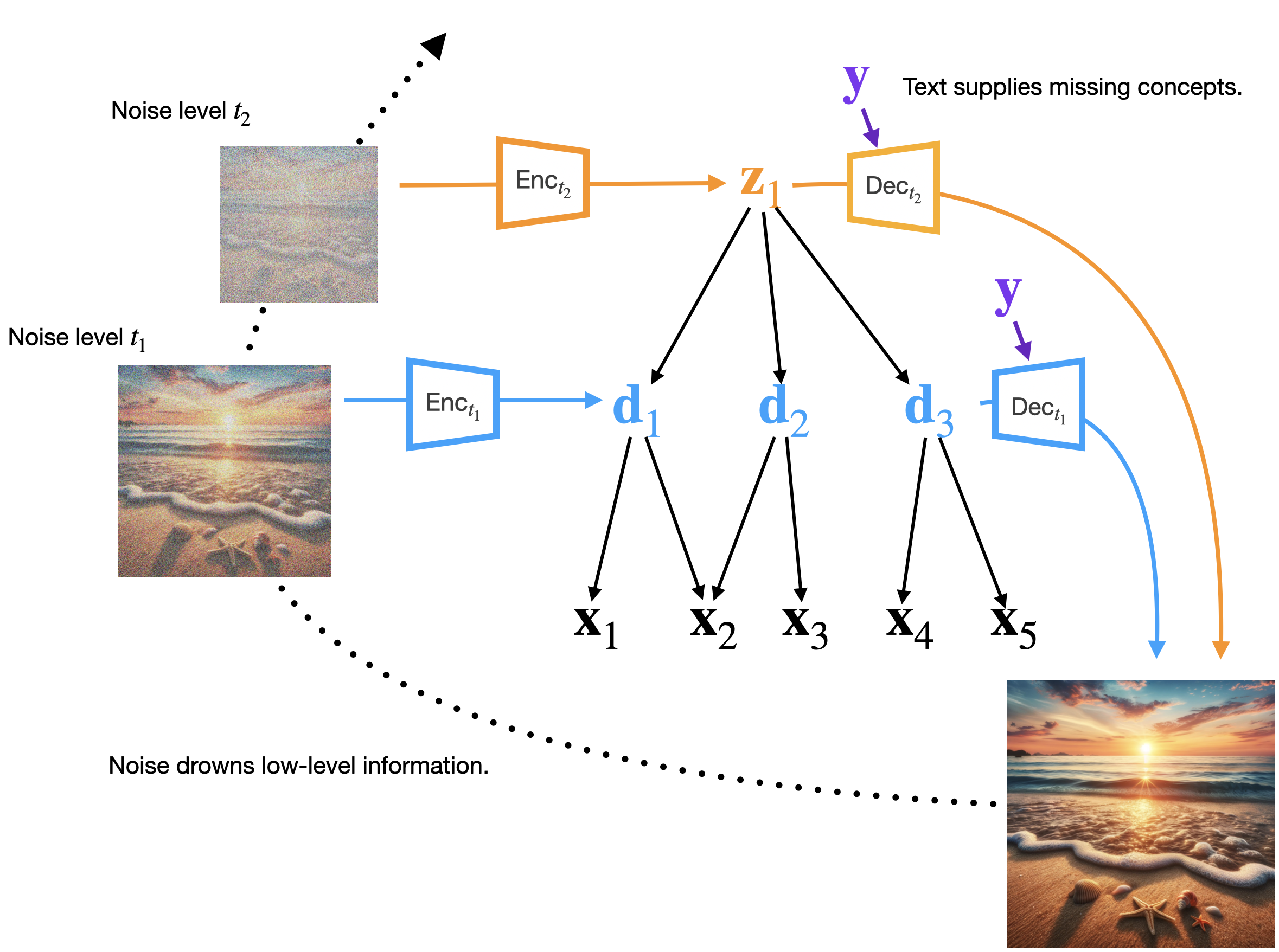
Figure 3: Diffusion models estimate the latent hierarchical model. Different noise levels correspond to different concept levels. To avoid cluttering, we leave out vector quantization.

Denoising objectives.

As discussed, diffusion training can be viewed as denoising the corrupted embedding $\tilde{\mathbf{d}}$ to restore noiseless $\mathbf{d}$ [47, 48, 49, 54] for a designated denoising model $f_{t}$ at noise level $t$:

$$\operatorname*{arg\,max}_{f_{t}}{\mathbb{E}}_{\mathbf{d},\tilde{\mathbf{d}}_{t}\sim\mathbb{Q}_{t}(\tilde{\mathbf{d}}_{t}|\mathbf{d})}\left[\mathbb{P}_{f_{t}}(\mathbf{d}|\tilde{\mathbf{d}}_{t},\mathbf{y})\right],$$ (2)

where $\mathbf{y}$ denotes the text prompt. Under this objective, the model is supposed to compress the noisy view $\tilde{\mathbf{d}}_{t}$ to extract a clean, high-level representation, together with additional information from the text $\mathbf{y}$, to reconstruct the original embedding $\mathbf{d}$. Formally, the denoising model $f_{t}:=f_{\text{dec},t}\circ f_{\text{enc},t}$ performs auto-encoding $\mathbf{z}_{\mathcal{S}(t)}=f_{\text{enc},t}(\tilde{\mathbf{d}}_{t})$ and $\hat{\mathbf{d}}=f_{\text{dec},t}(\mathbf{z}_{\mathcal{S}(t)},\mathbf{y})$, where we use $\mathcal{S}(t)$ to indicate the dependence on the noise level $t$. We can view the compressed representation $\mathbf{z}_{\mathcal{S}(t)}$ as a set of high-level latent variables in the hierarchical model: the encoder $f_{\text{enc},t}$ maps the noisy view $\tilde{\mathbf{d}}_{t}$ to high-level latent variables $\mathbf{z}_{\mathcal{S}_{t}}$ and the decoder $f_{\text{dec},t}$ assimilates the text information $\mathbf{y}$ and reconstructs the original view $\mathbf{d}$. In practice, $f_{t}$ is implemented as a single model (e.g., UNets) paired with time embeddings. We visualize this process in Figure 3.

Noise levels and hierarchical levels.

Intuitively, the noise level controls the amount of semantic information remaining in $\tilde{\mathbf{d}}_{t}$. For instance, a high noise level $t$ drowns the bulk of the low-level concepts in $\mathbf{d}$, leaving only sparse high-level concepts in $\tilde{\mathbf{d}}_{t}$. In this case, the diffusion representation $\mathbf{z}_{\mathcal{S}(t)}$ estimates a high concept level in the hierarchical model. In Figure 3, a high noise level may destroy low-level concepts, such as the sand texture and the waveforms, while preserving high-level concepts, such as the beach and the sunrise. In Section 6.1, we follow Park et al. [52] to demonstrate diffusion representation’s semantic levels under different noise levels.

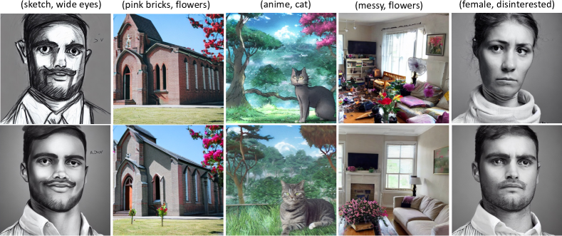
Figure 4: Hierarchical Concept Ordering. We inject concepts of distinct abstraction levels into the generating process at different time steps. In the top row, the concept injection follows the hierarchical order, which renders injected concepts faithfully. The bottom row reverses the hierarchical order and cannot incorporate concepts properly. More examples in Figure A5.

Theory and practice.

We connect LD training and estimating latent variables in the hierarchical model in an intuitive sense. Our theory focuses on the fundamental conditions on the data-generating process and do not directly translate to the guarantees for LD, which would require nontrivial assumptions on LD and we leave as future work. That said, our conditions naturally give implications on the algorithm design. For instance, a sparsity constraint on the decoding model may facilitate the identification condition that variables influence each other sparsely (e.g., pure children in Condition 3.7). In Section 6.2, we show such sparsity constraints are beneficial for concept extraction. We hope that our new perspective can provide more novel insights into advancing practical algorithms.

6 Real-world Experiments

6.1 Visualizing Hierarchical Concept Structures

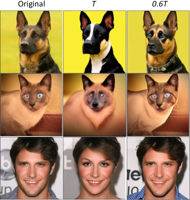
Figure 5: Semantic latent space in the diffusion model. We modify the diffusion model’s representation (UNet encoder’s output) along principal directions at diffusion time steps $T$ and $0.6T$. Structure changes indicates the semantic property of the representation and manipulation at the early time $T$ induces global concept shifts. More examples in Figure A6.

In this section, we show that latent representations at different diffusion steps correspond to different levels of the hierarchical causal model. We select concept pairs, each with higher-level and lower-level concepts. For example, in (“sketch,” “wide eyes”), “sketch” is more global, while “wide eyes” is more local. We alter the text prompt during diffusion generation for concept injection, appending “in a sketch style” to inject “sketch” (see Appendix A5 for prompts). In Figure 4, global concepts are successfully injected at early diffusion steps and local ones at late steps (top row). Reversing this order fails, as shown in the bottom row. For example, injecting “sketch” early and “wide eyes” late renders both correctly, but the global concept “sketch” is absent under the reverse injection order. This supports our theory that concepts are hierarchically organized, with higher-level concepts related to earlier diffusion steps.

Further, we support our interpretations in Section 5 that diffusion representation can be viewed as concept embeddings, and it corresponds to high-level concepts for high noise levels. Following Park et al. [52], we modify the diffusion representation along certain directions found unsupervisedly. We can observe that this manipulation gives rise to semantic concept changes rather than entangled corruption Figure 5. Editing the latent representation at early steps corresponds to shifting global concepts. In Figure 5, the latent representation in earlier steps (step $T$) determines breeds (the top row), species (the middle row), and gender (the bottom row). In contrast, the latent representation in later steps (step $0.6T$) correlates with the dog collar, cat eyes, and shirt patterns. Implementation details and additional results are provided in Appendix A5.

6.2 Causal Sparsity for Concept Extraction

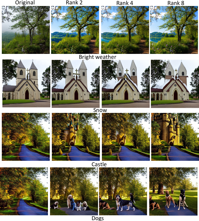
Figure 6: Concepts have varying levels of sparsity. We show that concepts of various abstraction levels correspond to different sparsity levels. For instance, bright weather is appropriately conveyed by a rank-$2$ LoRA and higher-rank LoRAs alter the background. Inadequate ranks fail to capture the concept faithfully and unnecessary ranks entangle the target concept with other attributes.

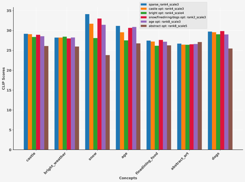
(a) CLIP scores.

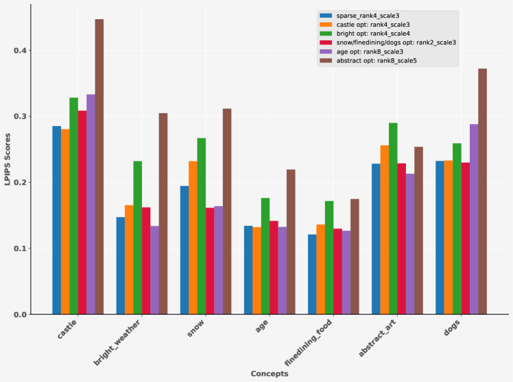
(b) LPIPS scores.

Figure 7: CLIP/LPIPS evaluation. We evaluate our approach and baselines at individual rank constraints. A high CLIP score is favorable as it indicates semantic alignment. A low LPIPS score is more favorable as it indicates minimal excessive changes. We compare our method “sparse” with the optimal fixed rank setting on each concept. For instance, “castle opt: rank4_scale3” indicates that the optimal setting for the concept “castle” is the LoRA of rank $4$ and scale $3$. With a adaptive rank selection, our approach outperforms or keeps up with the optimal fixed setting across different concepts. We repeat each training over three random seeds.

Recent work [55] shows that concepts can be extracted as low-rank parameter subspaces of LD models via LoRA [56]. This low-rankness limits the complexity of text-induced changes, resembling sparse influences from latent concepts to their descendants. Our theory suggests that different levels of concepts may require varying sparsity levels to capture. Figure 6 shows that indeed concepts at different abstraction levels have desirable representations at different ranks. For instance, the concept of bright weather is appropriately conveyed by a rank-$2$ LoRA and higher-rank LoRAs alter the background. The same observation occurs to other concepts, where inadequate ranks fail to capture the concept faithfully and unnecessary ranks entangle the target concept with other attributes.

Motivated by this, we design an adaptive sparsity selection mechanism for capturing concepts at different levels. Specifically, inspired by Ding et al. [57], we implement a sparsity constraint on the LoRA dimensionality for the model to select the LoRA rank at each module automatically (see Appendix A5 for details). Figure 7 presents the CLIP and LPIPS evaluation for the baseline and our approach, where the CLIP score evaluates the alignment between the image and the target description and the LPIPS score measures the structure change between the edited image and the original image. We can observe that under the sparsity constraint, our approach attains the highest CLIP score and the lowest LPIPS score when compared with the baselines of several ranks, indicating a higher level of alignment and a lower level of undesirable entanglement.

7 Conclusion

In this work, we cast the task of learning concepts as the identification problem of a discrete latent hierarchical model. Our theory provides conditions to guarantee the recoverability of discrete concepts. Further, we discuss and evaluate our framework’s implications on the working mechanism of diffusion models. Limitations: Although our theoretical framework provides a lens to interpret diffusion models, our conditions do not directly guarantee diffusion’s success, which would require nontrivial assumptions on the diffusion model. Also, Algorithm 1 can be expensive for large graphs, as the probability table’s size grows linearly with the number of discrete states. We leaving giving guarantees to diffusion models and more efficient graph learning algorithm as future work.

Appendix for
 
“Learning Discrete Concepts in Latent Hierarchical Causal Models”

Table of Contents

1

Appendix A1 Related Work

Concept learning.

In recent years, a significant strand of research has focused on employing labeled data to learn concepts in generative models’ latent space for image editing and manipulation [1, 2, 3, 4, 5, 6]. Concurrently, another independent research trajectory has been exploring unsupervised concept discovery and its potential to learn more compositional and transferable models, as shown in Burgess et al. [7], Locatello et al. [8], Du et al. [9, 10], Liu et al. [11]. These prior works focus on the empirical methodological development of concept learning by proposing novel neural network architectures and training objectives, with limited discussion on the theoretical aspect. In contrast, our work investigates the theoretical foundation of concept learning. Specifically, we formulate concept learning as an identification problem for a discrete latent hierarchical model and provide conditions under which extracting concepts is possible. Thus, the existing work and our work can be viewed as two complementary lines of research for concept learning.

Latent hierarchical models.

Complex real-world data distributions often possess a hierarchical structure among their underlying latent variables. On the theoretical front, Xie et al. [18], Huang et al. [19], Dong et al. [20] investigate identification conditions of latent hierarchical structures under the assumption that the latent variables are continuous and influence each other through linear functions. Kong et al. [58] extends the functional class to the nonlinear case over continuous variables. Pearl [21], Zhang [26], Choi et al. [22], Gu and Dunson [23] study fully discrete cases and thus fall short of modeling the continuous observed variables like images. Specifically, Pearl [21], Zhang [26], Choi et al. [22] focus on the latent trees in which every pair of variables is connected through exactly one undirected path. Gu and Dunson [23] assume a multi-level DAG [59] in which variables can be partitioned into disjoint groups (i.e., levels), such that all edges are between adjacent levels, with the observed variables as the bottom level (i.e., leaf nodes). In contrast, we show that we can not only extract discrete components from continuous observed variables but also uncover higher-level concepts and their interactions. Our graphical conditions admit multiple paths within each pair of latent variables, flexible hierarchical structures that are not necessarily multi-level, and flat structures in which all latent variables are adjacent to observed variables [24]. On the empirical side, prior work [60] improves the inference model of vanilla VAEs by combining bottom-up data-dependent likelihood terms with prior generative distribution parameters. Zhao et al. [61] assign more expressive (deeper) neural modules to higher-level variables to learn a more disentangled generative model. Li et al. [62] present a VAE architecture and clustering approaches to empirical estimate latent tree structures. Leeb et al. [63] propose to feed latent variable partitions into different decoder neural network layers and remove the prior regularization term to enable high-quality generation. Like our work, Ross and Doshi-Velez [64] consider discrete latent variables. However, their focus is on empirical evaluation benchmarks and metrics, without touching on the theoretical formulation of this task. Unlike these efforts, our work concentrates on the formalization of the data-generating process and the theoretical understanding. Thus, these two lines complement each other.

Latent variable identification.

Identifying latent variables under nonlinear transformations is central to representation learning on complex unstructured data. Khemakhem et al. [33, 32], Hyvarinen and Morioka [30], Hyvarinen et al. [31] assume the availability of auxiliary information (e.g., domain/class labels) and that the latent variables’ probability density functions have sufficiently different derivatives over domains/classes. However, many important concepts (e.g., object classes) are inherently discrete. Since latent variables are not equipped with differentiable density functions, identifying these concepts necessitates novel techniques. Our theory requires neither domain/class labels nor differentiable density functions and can accommodate discrete variables readily. Another line of studies [65, 66] refrains from the auxiliary information by making sparsity and mechanistic independence assumptions over latent variables, disregarding causal structures among the latent variables. Moreover, images may comprise abstract concepts and convey sophisticated interplay among concepts at various levels of abstraction. In this work, we address these limitations by formulating the concept space as a discrete hierarchical causal model, capturing concepts at distinct levels and their causal relations.

Latent diffusion understanding.

Diffusion probabilistic models [67, 68, 28, 69, 70, 71] have recently become the workhorse for state-of-the-art image generation. Diffusion models’ empirical success sparked a plethora of efforts to probe into their empirical properties. Kwon et al. [72], Park et al. [52] discover that the UNet bottleneck representation exhibits highly structured semantic properties, traversing over which manipulates the generated image in a meaningful manner. Choi et al. [73], Daras and Dimakis [74], Wu et al. [75], Sclocchi et al. [76] realize that early/late diffusion steps at the inference correlate with coarse/fine features in the output. Recently, Gandikota et al. [55] showcase that concepts are encoded by low-rank influences in latent diffusion models. The theoretical insights in our work consolidate these apparently separate strands of empirical observations and also lead to new understandings that could enhance empirical methodologies.

Appendix A2 Proof for Theorem 3.4

See 3.3 See 3.4

Proof of Theorem 3.4 Part 1.

The estimate $\hat{\mathbf{d}}$ and the true variable $\mathbf{d}$ are related through the map $[\hat{\mathbf{d}},\hat{\mathbf{c}}]=\hat{g}^{-1}\circ g(\mathbf{d},\mathbf{c})$. In the following, we show that the induced relation between $\mathbf{d}$ and $\hat{\mathbf{d}}$ is invertible under Condition 3.3-ii. The estimated generating process respects the conditions on the true generating process.

We denote that support of the estimate $\hat{\mathbf{d}}$ as $\hat{\Omega}^{(d)}$. First, we show by contradiction that for each state $k\in\Omega^{(d)}$, $k$ corresponds to at most one state $\hat{k}\in\hat{\Omega}^{(d)}$ of the estimate $\hat{\mathbf{d}}$.

Suppose that $k$ corresponds to two distinct states $\hat{k}_{1}$ and $\hat{k}_{2}$. That is, there exist $\mathbf{c}_{1},\mathbf{c}_{2}\in\mathcal{C}$ and $\hat{\mathbf{c}}_{1},\hat{\mathbf{c}}_{2}\in\hat{\mathcal{C}}$, such that $\hat{g}^{-1}\circ g(k,\mathbf{c}_{1})=[\hat{k}_{1},\hat{\mathbf{c}}_{1}]$ and $\hat{g}^{-1}\circ g(k,\mathbf{c}_{2})=[\hat{k}_{2},\hat{\mathbf{c}}_{2}]$. On one hand, As $g(k,\cdot)$ is a continuous function and $\mathcal{C}$ is connected, the image $\mathcal{I}(k):=g(k,\mathcal{C})$ is a connected set. On the other hand, $\hat{\mathcal{I}}(k_{1}):=\hat{g}(\hat{k}_{1},\hat{\mathcal{C}})$ and $\hat{\mathcal{I}}(\hat{k}_{2}):=\hat{g}(\hat{k}_{2},\hat{\mathcal{C}})$ are two separate sets due to the invertibility and continuity of $\hat{g}$ and the openness of $\hat{\mathcal{C}}$. To see this, invertibility implies that $\hat{\mathcal{I}}(k_{1})$ and $\hat{\mathcal{I}}(k_{2})$ are disjoint. The fact that $\hat{g}$ is continuous over $\hat{\mathbf{c}}$ and has a continuous inverse over $\hat{\mathbf{c}}$ implies that $\hat{\mathcal{I}}(k_{1})$ and $\hat{\mathcal{I}}(k_{2})$ preserve the openness $\mathcal{C}$. The space formed by two disjoint open subspaces is disconnected. Since $k$ corresponds to $\hat{k}_{1}$ and $\hat{k}_{2}$, it follows that $\mathcal{I}(k)=\hat{\mathcal{I}}_{1}\cup\hat{\mathcal{I}}_{2}$ where $\hat{\mathcal{I}}_{1}$ and $\hat{\mathcal{I}}_{2}$ are nonempty subsets of $\hat{\mathcal{I}}_{\hat{k}_{1}}$ and $\hat{\mathcal{I}}_{\hat{k}_{2}}$ respectively and inherit their separability. As $\mathcal{I}(k)$ is a union of two nonempty separated sets, it is disconnected. This contradicts the connectedness of $\mathcal{I}(k)$. Therefore, for each state $k\in\Omega^{(d)}$, $k$ corresponds to at most one state $\hat{k}\in\hat{\Omega}^{(d)}$.

Having established that each state of $\mathbf{d}$ corresponds to at most one state of $\hat{\mathbf{d}}$, we now show that states $\hat{k}_{1}$, $\hat{k}_{2}$ of $\hat{\mathbf{d}}$ corresponding to distinct states $k_{1}\neq k_{2}$ of $\mathbf{d}$ must also be distinct, i.e., $\hat{k}_{1}\neq\hat{k}_{2}$ if $k_{1}\neq k_{2}$. Suppose that $\exists k_{1}\neq k_{2}$, such that the corresponding states $\hat{k}_{1}=\hat{k}_{2}$. We denote $\hat{k}:=\hat{k}_{1}=\hat{k}_{2}$ and two arbitrary points $\mathbf{x}_{1}:=g(k_{1},\mathbf{c}_{1})$ and $\mathbf{x}_{2}:=g(k_{2},\mathbf{c}_{2})$ from modes $k_{1}$ and $k_{2}$ respectively. As the two estimated discrete states collapse at $\hat{k}$, it follows that

$$\mathbf{x}_{1}=g(k_{1},\mathbf{c}_{1}) =\hat{g}(\hat{k},\hat{\mathbf{c}}_{1})$$ (3)

$$\mathbf{x}_{2}=g(k_{2},\mathbf{c}_{2}) =\hat{g}(\hat{k},\hat{\mathbf{c}}_{2}).$$ (4)

Since $\hat{g}(\hat{k},\cdot)$ is continuous and $\hat{\mathcal{C}}$ is a connected set, the image $\hat{g}(\hat{k},\hat{\mathcal{C}})$ is path-connected. Thus, we can find a path $f:[0,1]\to\mathcal{X}$ such that $f(0)=\mathbf{x}_{1}$ and $f(1)=\mathbf{x}_{2}$. Also, each point on the path $f$ has a positive probability density due to positive $\hat{p}(\hat{\mathbf{c}})$ and ${\mathbb{P}}\left(\hat{\mathbf{d}}=\hat{k}\right)$. However, the two images $g(k_{1},\mathcal{C})$ and $g(k_{2},\mathcal{C})$ are disconnected due to the invertibility of $g$ and $k_{1}\neq k_{2}$. On any path from $\mathbf{x}_{1}$ to $\mathbf{x}_{2}$, there exists points $\mathbf{x}_{0}$ such that the density is strictly zero due to the discrete structure of $\mathbf{d}$. Thus, we have arrived at a contradiction. We have shown that if $k_{1}\neq k_{2}$, the corresponding estimated states are distinct $\hat{k}_{1}\neq\hat{k}_{2}$.

Since for for each $k\in\Omega^{(d)}$, $k$ corresponds to at most one state $\hat{k}$ and distinct states $k_{1}$, $k_{2}$ give rise to distinct states $\hat{k}_{1}$, $\hat{k}_{2}$, we have proven that for each $k\in\Omega^{(d)}$, $k$ corresponds to exactly one estimated state $\hat{k}\in\hat{\Omega}^{(d)}$.

∎

Definition A1 (Mixture Oracles).

Let $\mathbf{x}$ be a set of observed variables and $\mathbf{d}\in\Omega^{(d)}$ be a discrete latent variable. The mixture model is defined as ${\mathbb{P}}\left(\mathbf{x}\right)=\sum_{k\in\Omega^{(d)}}{\mathbb{P}}\left(\mathbf{d}=k\right){\mathbb{P}}\left(\mathbf{x}|\mathbf{d}=k\right)$. A mixture oracle $\text{MixOracle}(\mathbf{x})$ takes ${\mathbb{P}}\left(\mathbf{x}\right)$ as input and returns the number of components $\left\lvert\Omega^{(d)}\right\rvert$, the weights ${\mathbb{P}}\left(\mathbf{d}=k\right)$ and the component ${\mathbb{P}}\left(\mathbf{x}|\mathbf{d}=k\right)$ for $k\in\Omega^{(d)}$.

Theorem A2 (Kivva et al. [24]).

Under Condition 3.1 and Condition 3.3-iii, on can reconstruct the bipartite graph $\Gamma$ between $\mathbf{d}$ and $\mathbf{x}$, and the joint distribution ${\mathbb{P}}\left(d_{1}=k_{1},\dots,d_{n_{d}}=k_{n_{d}}\right)$ from ${\mathbb{P}}\left(\mathbf{x}\right)$ and $\text{MixOracle}(\mathbf{x})$.

Proof of Theorem 3.4 Part 2.

Step 1

: Given the first result in Theorem 3.4, we can identify the discrete state index $k$ for each realization of $\mathbf{x}$ (up to permutations). Since we can do this to all realizations of $\mathbf{x}$ and we are given ${\mathbb{P}}\left(\mathbf{x}\right)$, we can compute the cardinality of the discrete subspace $|\Omega^{(d)}|$, the marginal distribution of each latent state ${\mathbb{P}}\left(\mathbf{d}=k\right)$, and the conditional distribution ${\mathbb{P}}\left(\mathbf{x}|\mathbf{d}=k\right)$ for $k\in\Omega^{(d)}$.

Step 2

: Step 1 shows the availability of the mixture oracle MixOracle (i.e., $|\Omega|$, ${\mathbb{P}}\left(\mathbf{d}=k\right)$, and ${\mathbb{P}}\left(\mathbf{x}|\mathbf{d}=k\right)$ ) as defined in Definition A1. Now, all conditions employed in Theorem A2 are ready, namely Condition 3.1, Condition 3.3 iii, and MixOracle (the consequence of step 1). The derivation in Kivva et al. [24] entails identifying a map from the discrete subspace state index $\mathbf{d}=k$ where $k\in\Omega^{(d)}$ to all discrete components’ state indices $[d_{1},\dots,d_{n_{d}}]=[k_{1},\dots,k_{n_{d}}]$ where $k_{i}\in\Omega^{(d)}_{i}$ is the state index of the $i$-th component $d_{i}$. Thus, we can utilize this map to identify the state index for each individual discrete variable $d_{i}$ from the global index $k$.

Step 3

: As stated in Step 2, all conditions in Theorem A2 hold in our problem. Since Theorem Theorem A2 additionally identifies the bipartite graph $\Gamma$ between $\{x_{1},x_{2},x_{3},\dots\}$ and$\{d_{1},d_{2},d_{3},\dots\}$, the same follows in our case.

∎

Appendix A3 Proof for Theorem 3.8

In this section, we present a proof for Theorem 3.8. Since all variables are discrete for this proof, for a set of variables $\mathbf{A}$, we adopt the notation $\mathbf{A}=i$ to indicate the joint state of all variables in $\mathbf{A}$.

As outlined in Section 3, we will derive Theorem 3.5 which serves as the bridge between the distributional information and the graphical information, equivalent to the role of Theorem A4 Sullivant et al. [39] in Dong et al. [20], Huang et al. [19].

To familiarize the reader with the context, we first introduce Theorem A4 and the involved graphical definitions treks A1, t-separation A2, and its connection between d-separation [77].

Definition A1 (Treks).

A trek $T_{i,j}$ in a DAG from vertex $i$ to $j$ consists of a directed path $P_{ki}$ from vertex $k$ to $i$ and a direct path $P_{kj}$ from vertex $k$ to $j$, where we refer to $P_{ki}$ as the $i$ side and $P_{kj}$ as the $j$ side.

Intuitively, a trek is a path containing at most one fork structure and no collider structures. Given this definition, a notion of t-separation is introduced [43], reminiscent of the classic d-separation.

Definition A2 (t-Separation).

Let $\mathbf{A}$, $\mathbf{B}$, $\mathbf{C}_{\mathbf{A}}$, and $\mathbf{C}_{\mathbf{B}}$ be subsets (not necessarily disjoint) of vertices in a DAG. Then $(\mathbf{C}_{\mathbf{A}},\mathbf{C}_{\mathbf{B}})$ t-separates $\mathbf{A}$ and $\mathbf{B}$ if every trek from $\mathbf{A}$ to $\mathbf{B}$ passes through either a vertex in $\mathbf{C}_{\mathbf{A}}$ on the $\mathbf{A}$ side of the trek or a vertex $\mathbf{C}_{\mathbf{B}}$ on the $\mathbf{B}$ side of the trek.

Theorem A3 (Equivalence between d-separation and t-separation [78]).

Suppose we have disjoint vertex sets $\mathbf{A}$, $\mathbf{B}$, and $\mathbf{C}$ in a DAG. Set $\mathbf{C}$ d-separates set $\mathbf{A}$ and set $\mathbf{B}$ if and only if there exists a partition $\mathbf{C}:=\mathbf{C}_{\mathbf{A}}\cup\mathbf{C}_{\mathbf{B}}$ such that $(\mathbf{C}_{\mathbf{A}},\mathbf{C}_{\mathbf{B}})$ t-separates $\mathbf{A}\cup\mathbf{C}$ and $\mathbf{B}\cup\mathbf{C}$.

Theorem A3 shows that one can reformulate d-separation with a special form of t-separation. Thus, t-separation is at least as informative as d-separation. Further, as detailed in Dong et al. [20], t-separation can provide more information when latent variables are involved, benefiting from Theorem A4 [39].

Theorem A4 (Covariance Matrices and Graph Structures [39]).

Given two sets of variables $\mathbf{A}$ and $\mathbf{B}$ from a linear model with graph $\mathcal{G}$, it follows that $\text{rank}(\Sigma_{\mathbf{A},{\mathbf{B}}})=\min\{\left\lvert\mathbf{L}\right\rvert:\mathbf{L}~{}\text{t-separates}~{}\mathbf{A}~{}\text{from}~{}\mathbf{B}~{}\text{in}~{}\mathcal{G}\}$, where $\Sigma_{\mathbf{A},{\mathbf{B}}}$ denotes the generic covariance matrix between $\mathbf{A}$ and $\mathbf{B}$.

Theorem A4 reveals that one can access local latent graph structures, i.e., the cardinality of the minimal separation set between two subsets of observed variables, through computable statistical quantities, e.g., covariance matrix ranks. Dong et al. [20] utilize these local latent graph structures, together with graphical conditions, to develop their identification theory for linear hierarchical models. Ideally, if we can access such local latent structures in the discrete hierarchical model, we can apply the same graph search procedure and theorems in Dong et al. [20] to identify the discrete model. Nevertheless, Theorem A4 relies on the linearity of the causal model (i.e., each causal edge represents a linear function), which doesn’t hold in the discrete case. This motivates us to derive a counterpart of Theorem A4 for discrete causal models.

To this end, we will introduce a classic theorem (Theorem A6) that connects the non-negative rank of a joint probability table with latent variable states.

Definition A5 (Non-negative Rank).

The non-negative rank of a non-negative matrix $A\in\mathbb{R}^{m\times n}$ is equal to the smallest number $p$ such there exists a non-negative $m\times p$-matrix $\mathbf{B}$ and a non-negative $p\times n$-matrix $\mathbf{C}$ such that $\mathbf{A}=\mathbf{B}\mathbf{C}$.

Theorem A6 (Non-negative Rank and Probability Matrix Decomposition [40]).

Let $\mathbf{P}\in\mathbb{R}^{m\times n}$ be a bi-variate probability matrix. Then its non-negative rank $\text{rank}_{+}(\mathbf{P})$ is the smallest non-negative integer $p$ such that $\mathbf{P}$ can be expressed as a convex combination of $p$ rank-one bi-variate probability matrices.

Given this machinery, we now derive Theorem 3.5 which provides equivalent information in discrete models as Theorem A4 in linear models. See 3.5

Proof.

We express the joint distribution table $\mathbf{P}_{\mathbf{A},\mathbf{B}}$ as

$$\mathbf{P}(\mathbf{A}=i,\mathbf{B}=j)=\sum_{r\in[R]}\mathbf{P}(\mathbf{A}=i|\mathbf{L}=r)\mathbf{P}(\mathbf{B}=j|\mathbf{L}=r)\mathbf{P}(\mathbf{L}=r),$$ (5)

where $R\in\mathbb{N}^{+}$ is the smallest possible value. This is always possible since we can assign $\mathbf{L}$ as either $\mathbf{A}$ or $\mathbf{B}$ and obtain a trivial expression.

We note that $\mathbf{A}\setminus\mathbf{L}$, $\mathbf{B}\setminus\mathbf{L}$, and $\mathbf{L}$ are disjoint because if $\mathbf{A}\cap\mathbf{B}$ is nonempty, it must be a subset of $\mathbf{L}$. Since the graph $\mathcal{G}$ is non-degenerate (Condition 3.1-i) and faithful (Condition 3.7-i), Equation 5 implies the graphical condition that $\mathbf{A}\setminus\mathbf{L}$ and $\mathbf{B}\setminus\mathbf{L}$ are d-separate given $\mathbf{L}$.

The equivalence relation in Theorem A3 implies that a partition of $\mathbf{L}$ t-separates $\mathbf{A}$ and $\mathbf{B}$. Thus, the minimal cardinality $R$ is equal to the smallest number of discrete states of $\mathbf{L}$ that t-separates $\mathbf{A}$ and $\mathbf{B}$. Moreover, Theorem A6 implies that the minimal number of states is equal to the non-negative rank of $\mathbf{P}_{\mathbf{A},\mathbf{B}}$, i.e., $R=\text{rank}^{+}(\mathbf{P}_{\mathbf{A},\mathbf{B}})$, which concludes our proof. ∎

With Theorem 3.5 in hand, we leverage existing structural identification results on linear hierarchical models (Theorem A14) to obtain the identification results of desire (Theorem 3.8).

We introduce formal definitions of linear models, pure children, and the minimal graph operator, which we refer to in the main text.

Definition A7 (Linear Causal Models [20, 19]).

A linear causal model is a DAG with variable set $\mathbf{V}$ and an edge set $\mathbf{E}$, where each causal variables $v$ is generated by its parents $\text{Pa}(v)$ through a linear function:

$$v_{i}:=\sum_{v_{j}\in\text{Pa}(v)}a_{i,j}v_{j}+\epsilon_{i},$$ (6)

where $a_{i,j}$ is the causal strength and $\epsilon_{i}$ is the exogenous variable associated with $v_{i}$.

Definition A8 (Pure Children).

A variable set $\mathbf{Y}$ are pure children of variables $\mathbf{X}$ in graph $\mathcal{G}$, iff $\text{Pa}_{\mathcal{G}}(\mathbf{Y})=\cup_{\mathsf{Y_{i}}\in\mathbf{Y}}\text{Pa}_{\mathcal{G}}(\mathsf{Y_{i}})=\mathbf{X}$ and $\mathbf{X}\cap\mathbf{Y}=\emptyset$. We denote the pure children of $\mathbf{X}$ in $\mathcal{G}$ by $\text{PCh}_{\mathcal{G}}(\mathbf{X})$.

Basically, the definition dictates that variable $\mathbf{Y}$ has no other parents than $\mathbf{X}$.

Definition A9 (Minimal-graph Operator [19, 20]).

We can merge atomic covers $\mathbf{L}$ into $\mathbf{P}$ in $\mathcal{G}$ if (i) $\mathbf{L}$ is a pure child of $\mathbf{P}$, (ii) all elements of $L$ and $P$ are latent and $|\text{Supp}(\mathbf{L})|=|\text{Supp}(P)|$, and (iii) the pure children of $\mathbf{L}$ form a single atomic cover, or the siblings of $\mathbf{L}$ form a single atomic cover. We denote such an operator as the minimal-graph operator $\mathcal{O}_{\min}(\mathcal{G})$.

This operator merges certain structural redundancies not detectable from rank information [19, 20] (Lemma A13). Please refer to Figure A1 for an example.

Definition A10 (Atomic Covers (Linear Models)).

Let $\mathbf{A}$ be a set of variables in $\mathcal{G}$ with $|\mathbf{A}|=k$, where $t$ of the $k$ variables are observed variables, and the remaining $k-t$ are latent variables. $\mathbf{A}$ is an atomic cover if $\mathbf{A}$ contains a single observed variable, or if the following conditions hold:

• There exists a set of atomic covers $\mathcal{C}$, with $\left\lvert\mathcal{C}\right\rvert\geq k+1-t$, such that $\cup_{\mathbf{C}\in\mathcal{C}}\mathbf{C}\subseteq\text{PCh}_{\mathcal{G}}(\mathbf{V})$ and $\forall\mathbf{C_{1}},\mathbf{C_{2}}\in\mathcal{C},\mathbf{C_{1}}\cap\mathbf{C_{2}}=\emptyset$.

• There exists a set of covers $\mathcal{N}$, with $\left\lvert\mathcal{N}\right\rvert\geq k+1-t$, such that every element in $\cup_{\mathbf{N}\in\mathcal{N}}\mathbf{N}$ is a neighbour of $\mathbf{V}$ and $(\cup_{\mathbf{N}\in\mathcal{N}}\mathbf{N})\cap(\cup_{\mathbf{C}\in\mathcal{C}}\mathbf{C})=\emptyset$.

• There does not exist a partition of $\mathbf{A}=\mathbf{A_{1}}\cup\mathbf{A_{2}}$ such that both $\mathbf{A_{1}}$ and $\mathbf{A_{2}}$ are atomic covers.

Theorem A11 (Linear Hierarchical Model Conditions).

1. [Rank Faithfulness]: All the rank constraints on the covariance matrices are entailed by the DAG.

2. [Basic Graphical Conditions] For any $\mathsf{L}\in\mathbf{V}$, $\mathsf{L}$ belongs to at least one atomic cover (Definition A10) in the linear model $\mathcal{G}$ (Definition A7) and no latent variable is involved in any triangle structure (i.e., three mutually adjacent variables).

3. [Graphical Condition on Colliders] In a latent graph $\mathcal{G}$, if (i) there exists a set of variables $\mathbf{C}$ such that every variable in $\mathbf{C}$ is a collider of two atomic covers $\mathbf{L_{1}}$, $\mathbf{L_{2}}$, and denote by $\mathbf{A}$ the minimal set of variables that d-separates $\mathbf{L_{1}}$ from $\mathbf{L_{2}}$, (ii) there is a latent variable in $\mathbf{L_{1}},\mathbf{L_{2}},\mathbf{C}$ or $\mathbf{A}$, then we must have $\left\lvert\mathbf{C}\right\rvert+\left\lvert\mathbf{A}\right\rvert\geq\left\lvert\mathbf{L_{1}}\right\rvert+\left\lvert\mathbf{L_{2}}\right\rvert$.

Definition A12 (Skeleton Operator [19, 20]).

Given an atomic cover $\mathbf{A}$ in a graph $\mathcal{G}$, for all $a\in\mathbf{A}$, $a$ is latent, and all $c\in\text{PCh}(\mathbf{A})$, such that $a$ and $c$ are not adjacent, we can draw an edge from $a$ to $c$. We denote such an operator as skeleton operator $\mathcal{O}_{s}(\mathcal{G})$.

The skeleton operator introduces additional edges to fully connect atomic clusters [19, 20], which are indistinguishable from the rank information (Lemma A13). Please refer to Figure A1 for an example.

Lemma A13 (Rank Invariance Huang et al. [19]).

The rank constraints are invariant with the minimal-graph operator and the skeleton operator; that is, $\mathcal{G}$ and $\mathcal{O}_{s}(\mathcal{O}_{\min}(\mathcal{G}))$ are rank equivalent.

Theorem A14 (Linear Hierarchical Model Identification [20]).

Suppose the $\mathcal{G}$ is a linear latent causal model (Definition A7) that satisfies Condition A11. Then the hierarchical causal model $\mathcal{G}$ is identifiable up to the Markov equivalent class of $\mathcal{O}_{s}(\mathcal{O}_{\min}(\mathcal{G}))$.

We note that linear model conditions (Condition A11) and discrete model conditions (Condition 3.7) differ mainly in the substitutes of variables in the linear models with states in the discrete models. This originates from the local graph structures we can access, i.e., states in Theorem 3.5 and variables in Theorem A4. The skeleton operator $\mathcal{O}_{\min}$ (Definition A12 is not necessary under Condition 3.7 since each cover represents a discrete variable whose states must all be connected to its neighbors.

We now present Theorem 3.8 and its proof. See 3.7 See 3.8

Proof.

We observe that the linearity condition (Definition A7) in Theorem A14 is only utilized to invoke Theorem A4 to access the cardinality of the smallest t-separation set between any two sets of observed variables in the linear model. Through this, the graph identification results in Theorem A14 are derived based on a graph search algorithm repeatedly querying partial graph structures under Condition A11.

For discrete models (Condition 3.1), Theorem 3.5 supplies partial graph structures equivalent to Theorem A4. The difference is that Theorem A4 returns the number of variables in the smallest t-separation set while Theorem 3.5 returns the number of states in the smallest t-separation set. Thus, running Algorithm 1 up to Step 1 (i.e., the original search algorithm Dong et al. [20] with a different rank oracle in Theorem 3.5 highlighted in blue) will return a graph with latent nodes representing discrete states. Algorithm 1 is guaranteed to correctly discover all the atomic covers (Theorem A14) and each atomic cover corresponds to a latent discrete variables (Condition 3.7-ii). Thus, we can obtain each true latent variable by merging all the latent nodes $\mathbf{A}_{L}$ in each atomic cover $\mathbf{A}$ into a discrete latent variable $z$ whose support cardinality $\left\lvert\text{Supp}(z)\right\rvert$ equals to the number of latent nodes $\left\lvert\mathbf{A}_{L}\right\rvert$. We highlight this procedure (Step 1 in Algorithm 1). Moreover, as all latent nodes (i.e., latent states) in an atomic cover belong to one discrete variable, these latent nodes in adjacent atomic covers must be fully connected. Thus, we do not need the skeleton operator $\mathcal{O}_{s}$ as for linear models (Theorem A14). This concludes our proof for Theorem 3.8.

∎

Theorem 3.9 follows the same reasoning as in Theorem 3.8, with the main difference in organizing latent nodes/states into latent discrete variables.

Condition A15 (Discrete Hierarchical Model Conditions for Identifical Supports).

1. [Faithfulness]: All the conditional independence relations are entailed by the DAG.

2. [Basic Graphical Conditions]: Each latent variable $z\in\mathbf{Z}$ belongs to at least one atomic cover in $\mathcal{G}$ and no $z$ is involved in any triangle structure (i.e., three mutually adjacent variables).

3. [Graphical Condition on Colliders]: In a latent graph $\mathcal{G}$, if (i) there exists a set of variables $\mathbf{C}$ such that every variable in $\mathbf{C}$ is a collider of two atomic covers $\mathbf{L_{1}}$, $\mathbf{L_{2}}$, and denote by $\mathbf{A}$ the minimal set of variables that d-separates $\mathbf{L_{1}}$ from $\mathbf{L_{2}}$, (ii) there is a latent variable in $\mathbf{L_{1}},\mathbf{L_{2}},\mathbf{C}$ or $\mathbf{A}$, then we must have $\left\lvert\text{Supp}(\mathbf{C})\right\rvert+\left\lvert\text{Supp}(\mathbf{A})\right\rvert\geq\left\lvert\text{Supp}(\mathbf{L_{1}})\right\rvert+\left\lvert\text{Supp}(\mathbf{L_{2}})\right\rvert$.

See 3.9

Proof.

The bulk of the proof overlaps with the proof of Theorem 3.8. Following the same reasoning of the proof of Theorem 3.8, we can obtain a graph with latent nodes representing discrete states before Step 1 and Step 1 in Algorithm 1. Under the identical support condition in Theorem 3.9, we can directly group every $K$ states in an atomic cover into a latent variable as in Algorithm 1-Step 1. Since the true latent variable cardinality is known to be identical, we don’t need Condition 3.1-ii, iii to ensure the structure is well defined. Under Condition A15, each atomic cover may contain multiple discrete latent variables, depending on the cover size. It could be possible that one latent variable is not connected to all latent variables in an adjacent atomic cover, as in the linear model case. However, this difference cannot be detected from the rank information (Lemma A13). Thus, we need to retain the skeleton operator $\mathcal{O}_{s}$ inherited from Theorem A14 This concludes our proof for Theorem 3.9. ∎

(a) $\mathcal{G}$

(b) $\mathcal{O}_{\min}(\mathcal{G})$

(c) $\mathcal{O}_{s}(\mathcal{O}_{\min}(\mathcal{G}))$

Figure A1: The discrete graph $\mathcal{G}$ satisfies conditions in Theorem 3.9 (i.e., identical supports). After applying the minimal-graph operator to the graph $\mathcal{G}$, $z_{4}$ is merged to its parent $z_{5}$, and the rank constraints do not change. After applying the skeleton operator to the graph in (b), $z_{1}$ has an edge to $d_{7}$ and $z_{3}$ has an edge to $d_{1}$. We adopt this example from Huang et al. [19].

Input : Samples from all $n$ observed variables $\mathbf{X}_{\mathcal{G}}$

Output : Markov equivalence class $\mathcal{G^{\prime}}$

1 def LatentVariableCausalDiscovery($\mathbf{X}_{\mathcal{G}}$):

2       Phase 1: $\mathcal{G^{\prime}}$ = FindCISkeleton($\mathbf{X}_{\mathcal{G}}$) (Algorithm 2);

3       for  Each $\mathcal{Q}$, a group of overlapping maximal cliques, in $\mathcal{G^{\prime}}$ do

4             Set an empty graph $\mathcal{G^{\prime\prime}}$, $\mathbf{X}_{\mathcal{Q}}=\cup_{\mathbf{Q}\in\mathcal{Q}}\mathbf{Q}$, $\mathbf{N}_{\mathcal{Q}}=\{\mathsf{N}:\exists\mathsf{X}\in\mathbf{X}_{\mathcal{Q}}~{}\text{s.t.}~{}\mathsf{N},\mathsf{X}~{}\text{are adjacent in}~{}\mathcal{G^{\prime}}\}$;

5             Phase 2: $\mathcal{G^{\prime\prime}}$ = FindCausalClusters($\mathcal{G^{\prime\prime}}$, $\mathbf{X}_{\mathcal{Q}}\cup\mathbf{N}_{\mathcal{Q}}$) (Algorithm 3);

6             Phase 3: $\mathcal{G^{\prime\prime}}$ = RefineCausalClusters($\mathcal{G^{\prime\prime}}$, $\mathbf{X}_{\mathcal{Q}}\cup\mathbf{N}_{\mathcal{Q}}$) (Algorithm 5);

7             Transfer the estimated DAG $\mathcal{G^{\prime\prime}}$ to the Markov equivalence class and update $\mathcal{G^{\prime}}$ by $\mathcal{G^{\prime\prime}}$;

8            

9      Orient remaining causal directions that can be inferred from v structures;

10       Theorem 3.8: replace each cover $\mathbf{A}$ to a discrete variable $z$ with $\left\lvert\text{Supp}(z)\right\rvert:=\left\lvert\mathbf{A}_{L}\right\rvert$ & update $\mathcal{G}^{\prime}$ ;

11       Theorem 3.9: convert each cover $\mathbf{A}$ to $\log_{K}(\left\lvert\mathbf{A}_{L}\right\rvert)$ discrete variables of cardinality $K$ & update $\mathcal{G}^{\prime}$ ;

12       return $\mathcal{G^{\prime}}$

Algorithm 1 The overall procedure for Rank-based Discrete Latent Causal Model Discovery. [20] We denote the latent nodes in an atomic cover $\mathbf{A}$ as $\mathbf{A}_{L}$ and all observed nodes in the model $\mathcal{G}$ as $\mathbf{X}_{\mathcal{G}}$. We use blue color to highlight our modifications needed for Theorem 3.8 and Theorem 3.9 respectively.

Input : Samples from observed variables $\mathbf{X}_{\mathcal{G}}$

Output : CI skeleton $\mathcal{G^{\prime}}$

1 def Stage1PC($\mathbf{X}_{\mathcal{G}}$):

2       Initialize a complete undirected graph $\mathcal{G^{\prime}}$ on $\mathbf{X}_{\mathcal{G}}$;

3       repeat

4             repeat

5                   Select an ordered pair $\mathsf{X},\mathsf{Y}$ that are adjacent in $\mathcal{G^{\prime}}$, s.t., $|\text{Adj}_{\mathcal{G^{\prime}}}(\mathsf{X})\backslash\{\mathsf{Y}\}|\geq n$;

6                   Select a subset $\mathbf{S}\subseteq\text{Adj}_{\mathcal{G^{\prime}}}(\mathsf{X})\backslash\{\mathsf{Y}\}$ s.t., $|\mathbf{S}|=n$;

7                   If ${\color[rgb]{0,0,1}{\text{rank}^{+}(\mathbf{P}_{\{\mathsf{X}\}\cup\mathbf{S},\{\mathsf{Y}\}\cup\mathbf{S}})}}=|\mathbf{S}|$, delete the edge between $\mathsf{X}$ and $\mathsf{Y}$ from $\mathcal{G^{\prime}}$ and record $\mathbf{S}$ in $\text{Sepset}(\mathsf{X},\mathsf{Y})$ and $\text{Sepset}(\mathsf{Y},\mathsf{X})$.;

8                  

9            until all $\mathsf{X},\mathsf{Y}$ s.t., $|\text{Adj}_{\mathcal{G^{\prime}}}(\mathsf{X})\backslash\{\mathsf{Y}\}|\geq n$ and all $\mathbf{S}\subseteq\text{Adj}_{\mathcal{G^{\prime}}}(\mathsf{X})\backslash\{\mathsf{Y}\}$, $|\mathbf{S}|=n$, tested.;

10            n:=n+1;

11            

12      until no adjacent $\mathsf{X},\mathsf{Y}$ s.t., $|\text{Adj}_{\mathcal{G^{\prime}}}(\mathsf{X})\backslash\{\mathsf{Y}\}|<n$;

13      return $\mathcal{G^{\prime}}$

Algorithm 2 Phase1: FindCISkeleton [20] (Stage 1 of PC [43]). We denote the joint probability table between two sets $\mathbf{A}$ and $\mathbf{B}$ as $\mathbf{P}_{\mathbf{A},\mathbf{B}}$, the adjacent nodes as $\text{Adj},$the non-negative rank with $\text{rank}^{+}$, and the collection of d-separation sets as Sepset. We use blue color to highlight our modifications.

Input : Samples from $n$ observed variables $\mathbf{X}_{\mathcal{G}}$

Output : Graph $\mathcal{G^{\prime}}$

1 def FindCausalClusters($\mathcal{G^{\prime}}$, $\mathbf{X}_{\mathcal{G}}$):

       Active set $\mathcal{S}\leftarrow\mathcal{X}_{\mathcal{G}}=\{\{\mathsf{X_{1}}\},...,\{\mathsf{X_{n}}\}\}$, $k\leftarrow 1$ ;

        // $\mathcal{S}$ is a set of covers

2       repeat

             $\mathcal{G^{\prime}}$, $\mathcal{S}$, found = Search($\mathcal{G^{\prime}}$, $\mathcal{S}$, $\mathbf{X}_{\mathcal{G}}$, $k$) ;

              // Only when nothing can be found

             If $\text{found}=1$ then $k\leftarrow 1$ else $k\leftarrow k+1$ ;

              // udner current $k$ do we add $k$ by 1

3            

4      until $k$ is sufficiently large;

5      return $\mathcal{G^{\prime}}$;

6      

7 def Search($\mathcal{G^{\prime}}$, $\mathcal{S}$, $\mathbf{X}_{\mathcal{G}}$, $k$):

       Rank deficiency set $\mathbb{D}=\{\}$ ;

        // To store rank deficient combinations

8       for $\mathcal{T}\in\text{PowerSet}(\mathcal{S})$ (from $\mathcal{S}$ to $\emptyset$) do

             $\mathcal{S^{\prime}}\leftarrow(\mathcal{S}\backslash\mathcal{T})\cup(\cup_{\mathbf{T}\in\mathcal{T}}\text{PCh}_{\mathcal{G^{\prime}}}(\mathbf{T}))$ ;

              // Unfold $\mathcal{S}$ to get $\mathcal{S^{\prime}}$

9             for $t=k$ to $0$ do

10                   repeat

11                         Draw a set of $t$ observed covers $\mathcal{X}\subset\mathcal{S^{\prime}}\cap\mathcal{X}_{\mathcal{G}}$;

12                         repeat

13                               Draw a set of covers $\mathcal{C}\subset\mathcal{S^{\prime}}\backslash\mathcal{X}$, s.t., $||\mathcal{C}||=k-t+1$ and get $\mathcal{N}\leftarrow\mathcal{S^{\prime}}\backslash(\mathcal{X}\cup\mathcal{C})$;

14                              

15                              if ${\color[rgb]{0,0,1}{\text{rank}^{+}(\mathbf{P}_{\mathcal{C}\cup\mathcal{X},\mathcal{N}\cup\mathcal{X})}}}=k$ and NoCollider($\mathcal{C}$, $\mathcal{X}$, $\mathcal{N})$ then  Add $\mathcal{C}$ to $\mathbb{D}$ ;

16                              

17                        until all $\mathcal{C}$ exhausted;

18                        if $\mathbb{D}\neq\emptyset$ then

19                               for $\mathcal{D}_{i}\in\mathbb{D}$ do

20                                     if $|\text{Pa}_{\mathcal{G^{\prime}}}(\mathcal{D}_{i})\cup\mathbf{X}|=k$ then  $\mathbf{P}\leftarrow\text{Pa}_{\mathcal{G^{\prime}}}(\mathcal{D}_{i})\cup\mathbf{X}$ ;

21                                     else  Create new latent nodes $\mathbf{L}$, s.t., $\mathbf{P}\leftarrow\mathbf{L}\cup\text{Pa}_{\mathcal{G^{\prime}}}(\mathcal{D}_{i})\cup\mathbf{X}$ and $|\mathbf{L}|=k-|\text{Pa}_{\mathcal{G^{\prime}}}(\mathcal{D}_{i})\cup\mathbf{X}|$ ;

22                                     Update $\mathcal{G^{\prime}}$ by taking elements of $\mathcal{D}_{i}$ as the pure children of $\mathbf{P}$;

23                                     if $\mathbf{P}$ is atomic then  Update $\mathcal{S}\leftarrow(\mathcal{S}\backslash\mathcal{D}_{i})\cup\mathbf{P}$ ;

24                                    

                              return $\mathcal{G^{\prime}}$, $\mathcal{S}$, True ;

                                // Return to search with $k=1$

25                              

26                  until all $\mathcal{X}$ exhausted;

      return $\mathcal{G^{\prime}}$, $\mathcal{S}$, False ;

        // Return to search with $k\leftarrow k+1$

27      

Algorithm 3 Phase2: FindCausalClusters [20]. We use $||\cdot||$ to denote the number of all elements in a set of sets. We use the term "nodes" to refer to dummy variables that represent states rather than causal variables in the intermediate graph. We use blue color to highlight our modifications.

Input : $\mathcal{C}$, $\mathcal{X}$, $\mathcal{N}$

Output : Whether there exists $\mathbf{O}\in\mathcal{C}$ s.t., $\mathbf{O}$ is a collider of $\mathcal{C}\backslash\{\mathbf{O}\}$ and $\mathcal{N}$

1 def NoCollider($\mathcal{C}$, $\mathcal{X}$, $\mathcal{N}$):

2       for $c=1$ to $|\mathcal{C}|-1$ do

3             Draw $\mathcal{C^{\prime}}\subset\mathcal{C}$ s.t., $|\mathcal{C^{\prime}}|=c$;

4             repeat

5                   if ${\color[rgb]{0,0,1}{\text{rank}^{+}(\mathbf{P}_{\mathcal{C^{\prime}}\cup\mathcal{X},\mathcal{N}\cup\mathcal{X}})}}<||\mathcal{C^{\prime}}\cup\mathcal{X}||$ then  return False ;

6                  

7            until all $\mathcal{C^{\prime}}$ exhausted;

8      return True

Algorithm 4 NoCollider [20]. We use blue color to highlight our modifications.

Input : Graph $\mathcal{G}^{\prime}$

Output : Refined graph $\mathcal{G}^{\prime}$

1 def RefineCausalCLusters($\mathcal{G^{\prime}}$, $\mathbf{X}_{\mathcal{G}}$):

2       repeat

3             Draw an atomic cover $\mathbf{V}$ from $\mathcal{G^{\prime}}$;

4             Delete $\mathbf{V}$, neighbours of $\mathbf{V}$ that are latent, and all relating edges from $\mathcal{G^{\prime}}$ to get $\hat{\mathcal{G}}$;

5             $\mathcal{G^{\prime}}=\text{FindCausalClusters}(\hat{\mathcal{G}},\mathbf{X}_{\mathcal{G}})$;

6            

7      until No more $\mathbf{V}$ found and all $\mathbf{V}$ exhausted;

8      return $\mathcal{G^{\prime}}$

Algorithm 5 Phase3: RefineCausalClusters

Appendix A4 Synthetic Data Experiments

Data-generating processes.

For the hierarchical model $\mathcal{G}$, we randomly sample the parameters for each causal module, i.e., conditional distributions $p(z_{i}|\text{Parents}(z_{i}))$, according to a Dirichlet distribution over the states of $z_{i}$ with coefficient $1$. For simplicity, we follow condition in Theorem 3.9 and set the support size of latent variables to $2$. Like Kivva et al. [24], we build the generating process from $\mathbf{d}$ to the observed variables $\mathbf{x}$ (i.e., graph $\Gamma$) by a Gaussian mixture model where each state of the discrete subspace corresponds to one component/mode in the mixture model. We truncate the support of each component to improve the invertibility (Condition 3.3-ii). The graphs are exhibited in Figure A2 and Figure A3.

Metrics.

We adopt F1 score (i.e., $\frac{2\text{Precision}\cdot\text{Recall}}{\text{Precision}+\text{Recall}}$ ) to assess the graph learning results [20]. We compute recall and precision by checking whether the estimated model correctly retrieves edges in the true causal graph. Ranging between $0$ to $1$, high F1 scores indicate the search algorithm can recover ground-truth causal graphs. We repeat each experiment over at least $5$ random seeds.

Implementation details.

Our method comprise two stages: 1) learning the bottom-level discrete variable $\mathbf{d}$ and the bipartite graph $\Gamma$ from the observed variable $\mathbf{x}$; 2) learning the latent hierarchical model $\mathcal{G}$ given the bottom-level discrete variable $\mathbf{d}$ discovered in 1). For stage 1), we follow the clustering implementation in Kivva et al. [24] under the same hyper-parameter setup as in the original implementation. For stage 2), we apply Algorithm 1 to learn the hierarchical model $\mathcal{G}$. We opt for Step 1 in Algorithm 1 because we evaluate graphs with binary latent variables that meet the conditions of Theorem 3.9. Following Anandkumar et al. [41], Mazaheri et al. [42], we perform conventional rank computation rather than non-negative rank computation and find this replacement satisfactory. We conduct our experiments on a cluster of 64 CPUs. All experiments can be finished within half of an hour. The search algorithm implementation is adapted from Dong et al. [20].

Graphical structures.

Table 1 and Table 2 correspond to Figure A2 and Figure A3 respectively. As mentioned above, the graphs meet the conditions of Theorem 3.9 with the latent variable cardinality equal to two (binary variables).

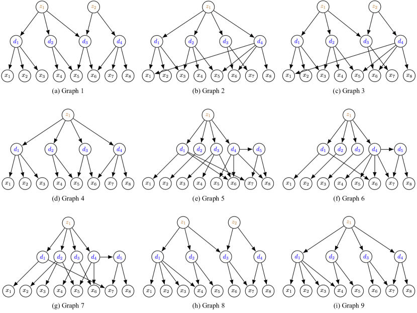
Figure A2: Causal graphs evaluated in Table 1. We denote the observed variables with $x$, the bottom-level latent discrete variables with $d$, and the high-level latent discrete variables with $z$.

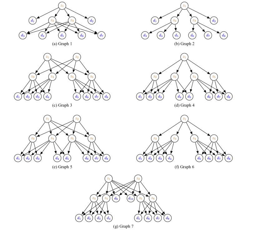
Figure A3: Causal graphs evaluated in Table 2. We denote the bottom-level latent discrete variables with $d$, and high-level latent discrete variables with $z$. Since baselines cannot extract discrete subspaces, we directly feed the algorithms the bottom-level discrete variables and test their structure learning performances.

Appendix A5 Real-world Experiments

A5.1 Implementation Details

We employ the pre-trained latent diffusion model [28] SD v1.4 across all our experiments. The inference process consists of $50$ steps.

For experiments in Section 6.1, we inject concepts by appending keywords to the original prompt. For instance, we inject the concept pair (“sketch”, “wide eyes”) in Figure 4 as follows. For the inference steps $0-10$, we feed the text prompt “A picture of a person”, for steps $10-20$, “a photo of a person, in a sketch style”, and for steps $20-50$, “a photo of a person, in a sketch style, with wide eyes”. For the reverse injection order (injecting “wide eyes” before “sketch”), we inject the following prompts at the three-step stages: “A picture of a person”, “a photo of a person, with wide eyes”, and “a photo of a person, with wide eyes, in a sketch style".

For experiments understanding the UNet’s latent presentation (Figure 5), we adopt the open-sourced code of Park et al. [52] .

For the attention sparsity experiment (Figure A4), we randomly generate images with the pre-train latent diffusion model and record its attention score across layers. To compute the relative sparsity, we select the threshold as $1/4096$ and compute the proportion of the attention scores over this threshold. For the attention visualization, we randomly select a head from the last attention module in the UNet architecture.

We follow the implementation of Gandikota et al. [55] to train concept sliders of various ranks. We adopt their evaluation protocol to obtain CLIP and LPIPS scores over $20$ randomly sampled images for each rank, concept, and scale combination. We evaluate ranks in $\{2,4,8\}$ and scales $\{1,2,3,4,5\}$. The rank selection technique, inspired by Ding et al. [57], involves multiplying each LoRA’s inner dimension with a scalar parameter and impose $\ell_{0}$ penalty on these scalar parameters. The weight on the $\ell_{0}$ penalty is selected from $\{1e-1,1e-2,1e-3,1e-4,1e-5\}$. We repeat each run for at least three random seeds.

We conduct all our experiments on 2 Nvidia L40 GPUs. Each image inference tasks the same time as in standard SD v1.4 for within two minutes. Each concept slider in Figure 7 takes around half an hour to train.

A5.2 Sparsity in the Hierarchical Model

To verify the sparse structure condition in Theorem 3.8, we view the attention sparsity in the LD model as an indicator of the connectivity between a specific hierarchical level and the bottom concept level. Figure A4 visualizes the attention sparsity of an LD model over diffusion steps and specific attention patterns in the model. We observe that the sparsity increases as the generative process progresses, which reflects that the connectivity between the hierarchical level ($\mathbf{z}_{\text{d},\mathcal{S}_{t}}$) and the bottom level variable ($\mathbf{d}$) becomes sparse and more local as we march down the hierarchical structure, which indicates a gradual localization of the concept.

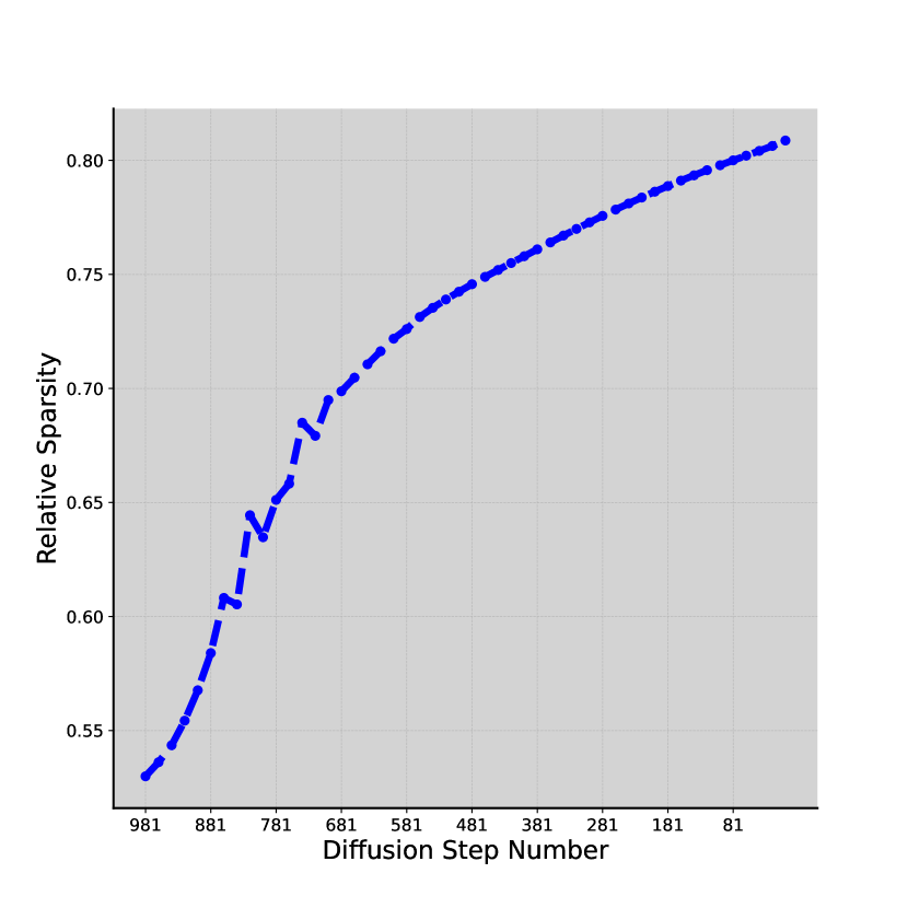
(a) Attention sparsity.

(b) Early step (index 1).

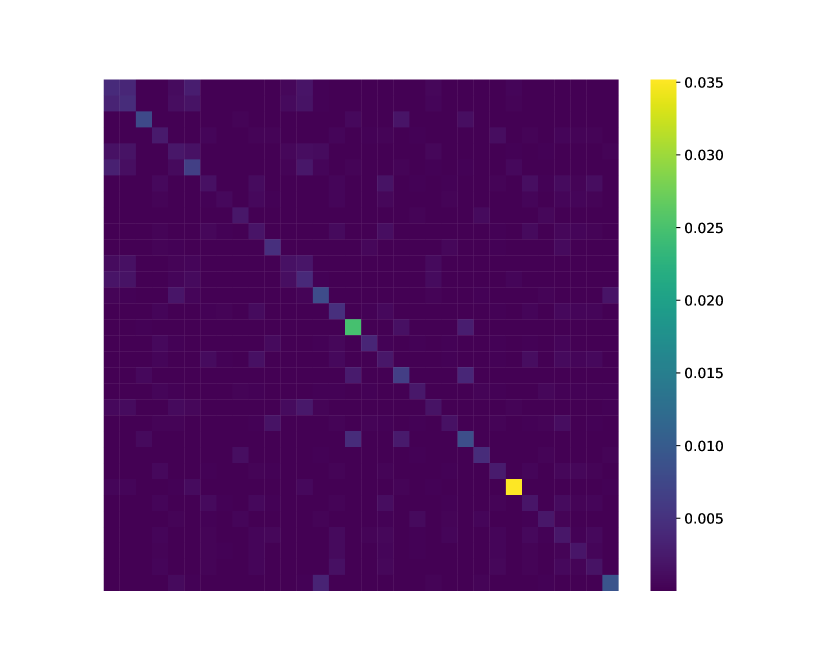
(c) Middle step (index 481).

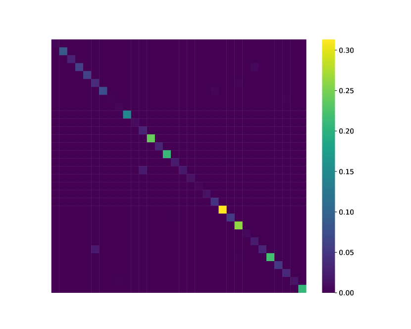
(d) Late step (index 981).

Figure A4: Sparsity patterns in latent diffusion models’ attention. We compute the proportions of the attention scores lower than a fixed threshold over the entire model. We can observe that the sparsity increases greatly towards small timesteps, i.e., the lower levels of the hierarchical model, which verifies our theory.

A5.3 More Examples

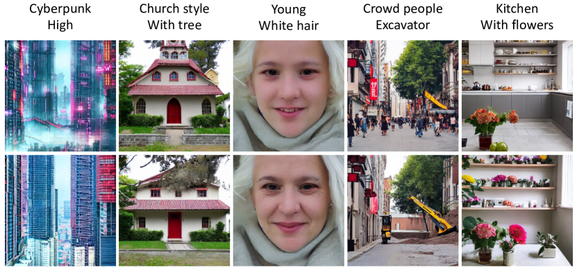
Figure A5: More examples for Figure 4.

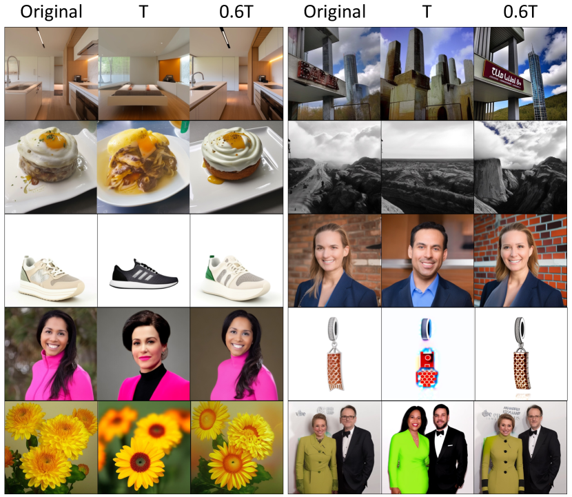
Figure A6: More examples for Figure 5.

References

- Gal et al. [2022] Rinon Gal, Yuval Alaluf, Yuval Atzmon, Or Patashnik, Amit Haim Bermano, Gal Chechik, and Daniel Cohen-or. An image is worth one word: Personalizing text-to-image generation using textual inversion. In The Eleventh International Conference on Learning Representations, 2022.
- Jahanian et al. [2019] Ali Jahanian, Lucy Chai, and Phillip Isola. On the" steerability" of generative adversarial networks. In International Conference on Learning Representations, 2019.
- Härkönen et al. [2020] Erik Härkönen, Aaron Hertzmann, Jaakko Lehtinen, and Sylvain Paris. Ganspace: Discovering interpretable gan controls. Advances in neural information processing systems, 33:9841–9850, 2020.
- Shen et al. [2020] Yujun Shen, Jinjin Gu, Xiaoou Tang, and Bolei Zhou. Interpreting the latent space of gans for semantic face editing. In Proceedings of the IEEE/CVF conference on computer vision and pattern recognition, pages 9243–9252, 2020.
- Wu et al. [2021] Zongze Wu, Dani Lischinski, and Eli Shechtman. Stylespace analysis: Disentangled controls for stylegan image generation. In Proceedings of the IEEE/CVF conference on computer vision and pattern recognition, pages 12863–12872, 2021.
- Ruiz et al. [2023] Nataniel Ruiz, Yuanzhen Li, Varun Jampani, Yael Pritch, Michael Rubinstein, and Kfir Aberman. Dreambooth: Fine tuning text-to-image diffusion models for subject-driven generation. In Proceedings of the IEEE/CVF Conference on Computer Vision and Pattern Recognition, pages 22500–22510, 2023.
- Burgess et al. [2019] Christopher P Burgess, Loic Matthey, Nicholas Watters, Rishabh Kabra, Irina Higgins, Matt Botvinick, and Alexander Lerchner. Monet: Unsupervised scene decomposition and representation. arXiv preprint arXiv:1901.11390, 2019.
- Locatello et al. [2020] Francesco Locatello, Dirk Weissenborn, Thomas Unterthiner, Aravindh Mahendran, Georg Heigold, Jakob Uszkoreit, Alexey Dosovitskiy, and Thomas Kipf. Object-centric learning with slot attention. In Advances in Neural Information Processing Systems 33 (NeurIPS 2020), 2020.
- Du et al. [2022a] Yilun Du, Shuang Li, Yash Sharma, Joshua B. Tenenbaum, and Igor Mordatch. Unsupervised learning of compositional energy concepts. In Proceedings of the International Conference on Learning Representations (ICLR 2022), 2022a.
- Du et al. [2022b] Yilun Du, Kevin Smith, Tomer Ulman, Joshua Tenenbaum, and Jiajun Wu. Unsupervised discovery of 3d physical objects from video. In Conference on Computer Vision and Pattern Recognition (CVPR 2022), 2022b.
- Liu et al. [2023] Nan Liu, Yilun Du, Shuang Li, Joshua B. Tenenbaum, and Antonio Torralba. Unsupervised compositional concepts discovery with text-to-image generative models. In Proceedings of the 2023 Conference on Neural Information Processing Systems (NeurIPS 2023), 2023.
- Koh et al. [2020] Pang Wei Koh, Thao Nguyen, Yew Siang Tang, Stephen Mussmann, Emma Pierson, Been Kim, and Percy Liang. Concept bottleneck models. In International conference on machine learning, pages 5338–5348. PMLR, 2020.
- Zarlenga et al. [2022] Mateo Espinosa Zarlenga, Pietro Barbiero, Gabriele Ciravegna, Giuseppe Marra, Francesco Giannini, Michelangelo Diligenti, Frederic Precioso, Stefano Melacci, Adrian Weller, Pietro Lio, et al. Concept embedding models. In NeurIPS 2022-36th Conference on Neural Information Processing Systems, 2022.
- Oikarinen and Weng [2022] Tuomas Oikarinen and Tsui-Wei Weng. Clip-dissect: Automatic description of neuron representations in deep vision networks. In ICLR 2022 Workshop on PAIR textasciicircum 2Struct: Privacy, Accountability, Interpretability, Robustness, Reasoning on Structured Data, 2022.
- Moayeri et al. [2023a] Mazda Moayeri, Keivan Rezaei, Maziar Sanjabi, and Soheil Feizi. Text-to-concept (and back) via cross-model alignment. In International Conference on Machine Learning, pages 25037–25060. PMLR, 2023a.
- Moayeri et al. [2023b] Mazda Moayeri, Keivan Rezaei, Maziar Sanjabi, and Soheil Feizi. Text2concept: Concept activation vectors directly from text. In Proceedings of the IEEE/CVF Conference on Computer Vision and Pattern Recognition, pages 3743–3748, 2023b.
- Radford et al. [2021] Alec Radford, Jong Wook Kim, Chris Hallacy, Aditya Ramesh, Gabriel Goh, Sandhini Agarwal, Girish Sastry, Amanda Askell, Pamela Mishkin, Jack Clark, et al. Learning transferable visual models from natural language supervision. In International conference on machine learning, pages 8748–8763. PMLR, 2021.
- Xie et al. [2022] Feng Xie, Biwei Huang, Zhengming Chen, Yangbo He, Zhi Geng, and Kun Zhang. Identification of linear non-gaussian latent hierarchical structure. In International Conference on Machine Learning, pages 24370–24387. PMLR, 2022.
- Huang et al. [2022] Biwei Huang, Charles Jia Han Low, Feng Xie, Clark Glymour, and Kun Zhang. Latent hierarchical causal structure discovery with rank constraints. Advances in Neural Information Processing Systems, 35:5549–5561, 2022.
- Dong et al. [2023] Xinshuai Dong, Biwei Huang, Ignavier Ng, Xiangchen Song, Yujia Zheng, Songyao Jin, Roberto Legaspi, Peter Spirtes, and Kun Zhang. A versatile causal discovery framework to allow causally-related hidden variables. In The Twelfth International Conference on Learning Representations, 2023.
- Pearl [1988] J. Pearl. Probabilistic Reasoning in Intelligent Systems: Networks of Plausible Inference. Morgan Kaufmann, 1988.
- Choi et al. [2011] Myung Jin Choi, Vincent YF Tan, Animashree Anandkumar, and Alan S Willsky. Learning latent tree graphical models. Journal of Machine Learning Research, 12:1771–1812, 2011.
- Gu and Dunson [2023] Yuqi Gu and David B. Dunson. Bayesian pyramids: Identifiable multilayer discrete latent structure models for discrete data. In Journal of the Royal Statistical Society Series B: Statistical Methodology, 2023.
- Kivva et al. [2021] Bohdan Kivva, Goutham Rajendran, Pradeep Ravikumar, and Bryon Aragam. Learning latent causal graphs via mixture oracles. Advances in Neural Information Processing Systems, 34:18087–18101, 2021.
- Drton et al. [2017] Mathias Drton, Shaowei Lin, Luca Weihs, and Piotr Zwiernik. Marginal likelihood and model selection for gaussian latent tree and forest models. Bernoulli, pages 1202–1232, 2017.
- Zhang [2004] Nevin L Zhang. Hierarchical latent class models for cluster analysis. The Journal of Machine Learning Research, 5:697–723, 2004.
- Anandkumar et al. [2013a] Animashree Anandkumar, Daniel Hsu, Adel Javanmard, and Sham Kakade. Learning linear bayesian networks with latent variables. In Sanjoy Dasgupta and David McAllester, editors, Proceedings of the 30th International Conference on Machine Learning, volume 28 of Proceedings of Machine Learning Research, pages 249–257, Atlanta, Georgia, USA, 17–19 Jun 2013a. PMLR. URL https://proceedings.mlr.press/v28/anandkumar13.html.
- Rombach et al. [2022] Robin Rombach, Andreas Blattmann, Dominik Lorenz, Patrick Esser, and Björn Ommer. High-resolution image synthesis with latent diffusion models. In Proceedings of the 2022 IEEE/CVF Conference on Computer Vision and Pattern Recognition (CVPR 2022), 2022.
- Kivva et al. [2022] Bohdan Kivva, Goutham Rajendran, Pradeep Ravikumar, and Bryon Aragam. Identifiability of deep generative models without auxiliary information. Advances in Neural Information Processing Systems, 35:15687–15701, 2022.
- Hyvarinen and Morioka [2016] Aapo Hyvarinen and Hiroshi Morioka. Unsupervised feature extraction by time-contrastive learning and nonlinear ica. Advances in neural information processing systems, 29, 2016.
- Hyvarinen et al. [2019] Aapo Hyvarinen, Hiroaki Sasaki, and Richard Turner. Nonlinear ica using auxiliary variables and generalized contrastive learning. In The 22nd International Conference on Artificial Intelligence and Statistics, pages 859–868. PMLR, 2019.
- Khemakhem et al. [2020a] Ilyes Khemakhem, Ricardo Monti, Diederik Kingma, and Aapo Hyvarinen. Ice-beem: Identifiable conditional energy-based deep models based on nonlinear ica. Advances in Neural Information Processing Systems, 33:12768–12778, 2020a.
- Khemakhem et al. [2020b] Ilyes Khemakhem, Diederik Kingma, Ricardo Monti, and Aapo Hyvarinen. Variational autoencoders and nonlinear ica: A unifying framework. In International Conference on Artificial Intelligence and Statistics, pages 2207–2217. PMLR, 2020b.
- Von Kügelgen et al. [2021] Julius Von Kügelgen, Yash Sharma, Luigi Gresele, Wieland Brendel, Bernhard Schölkopf, Michel Besserve, and Francesco Locatello. Self-supervised learning with data augmentations provably isolates content from style. Advances in neural information processing systems, 34:16451–16467, 2021.
- Kong et al. [2022] Lingjing Kong, Shaoan Xie, Weiran Yao, Yujia Zheng, Guangyi Chen, Petar Stojanov, Victor Akinwande, and Kun Zhang. Partial disentanglement for domain adaptation. In International Conference on Machine Learning, pages 11455–11472. PMLR, 2022.
- Arora et al. [2012] Sanjeev Arora, Rong Ge, and Ankur Moitra. Learning topic models–going beyond svd. In 2012 IEEE 53rd annual symposium on foundations of computer science, pages 1–10. IEEE, 2012.
- Arora et al. [2013] Sanjeev Arora, Rong Ge, Yonatan Halpern, David Mimno, Ankur Moitra, David Sontag, Yichen Wu, and Michael Zhu. A practical algorithm for topic modeling with provable guarantees. In International conference on machine learning, pages 280–288. PMLR, 2013.
- Gu [2022] Yuqi Gu. Blessing of dependence: Identifiability and geometry of discrete models with multiple binary latent variables. arXiv preprint arXiv:2203.04403, 2022.
- Sullivant et al. [2010] Seth Sullivant, Kelli Talaska, and Jan Draisma. Trek separation for gaussian graphical models. The Annals of Statistics, 38(3), June 2010. ISSN 0090-5364. doi: 10.1214/09-aos760. URL http://dx.doi.org/10.1214/09-AOS760.
- Cohen and Rothblum [1993] Joel E Cohen and Uriel G Rothblum. Nonnegative ranks, decompositions, and factorizations of nonnegative matrices. Linear Algebra and its Applications, 190:149–168, 1993.
- Anandkumar et al. [2012] A. Anandkumar, D. Hsu, F. Huang, and S. M. Kakade. Learning high-dimensional mixtures of graphical models, 2012.
- Mazaheri et al. [2023] Bijan Mazaheri, Spencer Gordon, Yuval Rabani, and Leonard Schulman. Causal discovery under latent class confounding. arXiv preprint arXiv:2311.07454, 2023.
- Spirtes et al. [2001] Peter Spirtes, Clark Glymour, and Richard Scheines. Causation, prediction, and search. MIT press, 2001.
- Xie et al. [2020] Feng Xie, Ruichu Cai, Biwei Huang, Clark Glymour, Zhifeng Hao, and Kun Zhang. Generalized independent noise condition for estimating latent variable causal graphs. Advances in Neural Information Processing Systems, 33:14891–14902, 2020.
- Lemeire and Janzing [2013] Jan Lemeire and Dominik Janzing. Replacing causal faithfulness with algorithmic independence of conditionals. Minds and Machines, 23:227–249, 2013.
- Vincent [2011] Pascal Vincent. A connection between score matching and denoising autoencoders. Neural computation, 23(7):1661–1674, 2011.
- Song and Ermon [2019] Yang Song and Stefano Ermon. Generative modeling by estimating gradients of the data distribution. Advances in neural information processing systems, 32, 2019.
- Vincent et al. [2008] Pascal Vincent, Hugo Larochelle, Yoshua Bengio, and Pierre-Antoine Manzagol. Extracting and composing robust features with denoising autoencoders. In Proceedings of the 25th international conference on Machine learning, pages 1096–1103, 2008.
- Vincent et al. [2010] Pascal Vincent, Hugo Larochelle, Isabelle Lajoie, Yoshua Bengio, Pierre-Antoine Manzagol, and Léon Bottou. Stacked denoising autoencoders: Learning useful representations in a deep network with a local denoising criterion. Journal of machine learning research, 11(12), 2010.
- Pathak et al. [2016] Deepak Pathak, Philipp Krahenbuhl, Jeff Donahue, Trevor Darrell, and Alexei A. Efros. Context encoders: Feature learning by inpainting, 2016.
- He et al. [2021] Kaiming He, Xinlei Chen, Saining Xie, Yanghao Li, Piotr Dollár, and Ross Girshick. Masked autoencoders are scalable vision learners, 2021.
- Park et al. [2023] Yong-Hyun Park, Mingi Kwon, Jaewoong Choi, Junghyo Jo, and Youngjung Uh. Understanding the latent space of diffusion models through the lens of riemannian geometry. Advances in Neural Information Processing Systems, 36:24129–24142, 2023.
- Esser et al. [2021] Patrick Esser, Robin Rombach, and Björn Ommer. Taming transformers for high-resolution image synthesis. In Proceedings of the IEEE/CVF Conference on Computer Vision and Pattern Recognition (CVPR 2021), 2021.
- Gu et al. [2022] Shuyang Gu, Dong Chen, Jianmin Bao, Fang Wen, Bo Zhang, Dongdong Chen, Lu Yuan, and Baining Guo. Vector quantized diffusion model for text-to-image synthesis, 2022.
- Gandikota et al. [2023] Rohit Gandikota, Joanna Materzyńska, Tingrui Zhou, Antonio Torralba, and David Bau. Concept sliders: Lora adaptors for precise control in diffusion models. arXiv preprint arXiv:2311.12092, 2023.
- Hu et al. [2021] Edward J. Hu, Yelong Shen, Phillip Wallis, Zeyuan Allen-Zhu, Yuanzhi Li, Shean Wang, Lu Wang, and Weizhu Chen. Lora: Low-rank adaptation of large language models. In Proceedings of the 2021 International Conference on Learning Representations (ICLR 2021), 2021.
- Ding et al. [2023] Ning Ding, Xingtai Lv, Qiaosen Wang, Yulin Chen, Bowen Zhou, Zhiyuan Liu, and Maosong Sun. Sparse low-rank adaptation of pre-trained language models. In Proceedings of the 2023 Conference on Empirical Methods in Natural Language Processing (EMNLP 2023), 2023.
- Kong et al. [2023] Lingjing Kong, Biwei Huang, Feng Xie, Eric Xing, Yuejie Chi, and Kun Zhang. Identification of nonlinear latent hierarchical models. Advances in Neural Information Processing Systems, 36, 2023.
- Anandkumar et al. [2013b] Animashree Anandkumar, Daniel Hsu, Adel Javanmard, and Sham Kakade. Learning linear bayesian networks with latent variables. In International Conference on Machine Learning, pages 249–257. PMLR, 2013b.
- Sønderby et al. [2016] Casper Kaae Sønderby, Tapani Raiko, Lars Maaløe, Søren Kaae Sønderby, and Ole Winther. Ladder variational autoencoders. Advances in neural information processing systems, 29, 2016.
- Zhao et al. [2017] Shengjia Zhao, Jiaming Song, and Stefano Ermon. Learning hierarchical features from deep generative models. In International Conference on Machine Learning, pages 4091–4099. PMLR, 2017.
- Li et al. [2018] Xiaopeng Li, Zhourong Chen, Leonard KM Poon, and Nevin L Zhang. Learning latent superstructures in variational autoencoders for deep multidimensional clustering. arXiv preprint arXiv:1803.05206, 2018.
- Leeb et al. [2022] Felix Leeb, Giulia Lanzillotta, Yashas Annadani, Michel Besserve, Stefan Bauer, and Bernhard Schölkopf. Structure by architecture: Structured representations without regularization. In The Eleventh International Conference on Learning Representations, 2022.
- Ross and Doshi-Velez [2021] Andrew Ross and Finale Doshi-Velez. Benchmarks, algorithms, and metrics for hierarchical disentanglement. In International Conference on Machine Learning, pages 9084–9094. PMLR, 2021.
- Brady et al. [2024] Jack Brady, Roland S. Zimmermann, Yash Sharma, Bernhard Schölkopf, Julius von Kügelgen, and Wieland Brendel. Provably learning object-centric representations. In International Conference on Learning Representations (ICLR 2024), 2024.
- Lachapelle et al. [2024] Sébastien Lachapelle, Divyat Mahajan, Ioannis Mitliagkas, and Simon Lacoste-Julien. Additive decoders for latent variables identification and cartesian-product extrapolation. Advances in Neural Information Processing Systems, 36, 2024.
- Sohl-Dickstein et al. [2015] Jascha Sohl-Dickstein, Eric A. Weiss, Niru Maheswaranathan, and Surya Ganguli. Deep unsupervised learning using nonequilibrium thermodynamics. In Proceedings of the International Conference on Machine Learning (ICML 2015), 2015.
- Ho et al. [2020] Jonathan Ho, Ajay Jain, and Pieter Abbeel. Denoising diffusion probabilistic models. In Advances in Neural Information Processing Systems 33 (NeurIPS 2020), 2020.
- Song et al. [2022] Jiaming Song, Chenlin Meng, and Stefano Ermon. Denoising diffusion implicit models. In International Conference on Learning Representations (ICLR 2022), 2022.
- Dhariwal and Nichol [2021] Prafulla Dhariwal and Alex Nichol. Diffusion models beat gans on image synthesis. In Advances in Neural Information Processing Systems 34 (NeurIPS 2021), 2021.
- Nichol and Dhariwal [2021] Alex Nichol and Prafulla Dhariwal. Improved denoising diffusion probabilistic models. In Proceedings of the International Conference on Machine Learning (ICML 2021), 2021.
- Kwon et al. [2022] Mingi Kwon, Jaeseok Jeong, and Youngjung Uh. Diffusion models already have a semantic latent space. In The Eleventh International Conference on Learning Representations, 2022.
- Choi et al. [2022] Jooyoung Choi, Jungbeom Lee, Chaehun Shin, Sungwon Kim, Hyunwoo Kim, and Sungroh Yoon. Perception prioritized training of diffusion models. In Proceedings of the IEEE/CVF Conference on Computer Vision and Pattern Recognition, pages 11472–11481, 2022.
- Daras and Dimakis [2022] Giannis Daras and Alexandros G Dimakis. Multiresolution textual inversion. arXiv preprint arXiv:2211.17115, 2022.
- Wu et al. [2023] Qiucheng Wu, Yujian Liu, Handong Zhao, Ajinkya Kale, Trung Bui, Tong Yu, Zhe Lin, Yang Zhang, and Shiyu Chang. Uncovering the disentanglement capability in text-to-image diffusion models. In Proceedings of the IEEE/CVF Conference on Computer Vision and Pattern Recognition, pages 1900–1910, 2023.
- Sclocchi et al. [2024] Antonio Sclocchi, Alessandro Favero, and Matthieu Wyart. A phase transition in diffusion models reveals the hierarchical nature of data. arXiv preprint arXiv:2402.16991, 2024.
- Pearl [2009] Judea Pearl. Causality. Cambridge university press, 2009.
- Di [2009] Yanming Di. t-separation and d-separation for directed acyclic graphs. preprint, 2009.