Kernel-based Minimal Distributed Charges: A Conformationally Dependent ESP-Model for Molecular Simulations

Abstract

A kernel-based method (kernelized minimal distributed charge model - kMDCM) to represent the molecular electrostatic potential (ESP) in terms of off-center point charges whose positions adapts to the molecular geometry. Using Gaussian kernels and atom-atom distances as the features, the ESP for water and methanol is shown to improve by at least a factor of two compared with point charge models fit to an ensemble of structures. Combining kMDCM for the electrostatics and reproducing kernels for the bonded terms allows energy-conserving simulation of 2000 water molecules with periodic boundary conditions on the nanosecond time scale.

University of Basel]Department of Chemistry, University of Basel, Klingelbergstrasse 80 , CH-4056 Basel, Switzerland. University of Basel]Department of Chemistry, University of Basel, Klingelbergstrasse 80 , CH-4056 Basel, Switzerland. University of Basel]Department of Chemistry, University of Basel, Klingelbergstrasse 80 , CH-4056 Basel, Switzerland. University of Basel]Department of Chemistry, University of Basel, Klingelbergstrasse 80 , CH-4056 Basel, Switzerland.

1 Introduction

Empirical energy functions (EEFs) constitute an important framework in state-of-the art characterization of the energetics and dynamics of molecular systems in the gas- and the condensed-phase.^{1, 2, 3} The success of EEFs is primarily owed to the speed with which energies and forces can be evaluated for a given arrangement of the atoms. In the most conventional formulation, EEFs distinguish between bonded and nonbonded energy contributions and the nonbonded interactions encompass van der Waals and electrostatic interactions.⁴ The electrostatic contributions are often conveniently described by atom-centered point charge (PC) models which can be considered as the first term of a multipolar expansion based on atom-centered moments.⁵

It has been long recognized that correctly capturing the anisotropy of the electrostatic (Coulomb) contributions to the total energy is mandatory for a realistic description of the intermolecular interactions.⁶ One possibility to achieve this is to represent the molecular electrostatic potential (ESP) as a superposition of atom-centered multipoles (MTPs) to given order. Often, this expansion is truncated at the atomic quadrupole moment for all atoms except hydrogens for which a PC representation is usually sufficient.^{7, 8, 9, 10} Alternatively, PC-based energy functions can be supplemented by off-center PCs to model the anisotropy of the ESP originating from an anisotropic electron density due to, for example, $\sigma-$holes¹¹ or lone pairs.

Besides charge anisotropy, intramolecular charge redistribution occurs as a consequence of changes in molecular geometry.¹² Such changes in the electron density lead to fluctuations in the electric dipole and higher molecular moments which affect, among others, the intensities of infrared (IR) spectra. Modelling such effects can be accomplished through conformationally dependent atom-centered multipoles.^{8, 13, 14} It was also found that the electric field around a molecule depends on all molecular degrees of freedom,^{15, 16} which cannot be described by simply translating and rotating a locally frozen electron density to a new spatial position and orientation. As an example, the molecular dipole moment of water is often cited to demonstrate the conformational dependence of the electrostatic potential,^{17, 18, 19} as fluctuations in the range of $\sim 50\%$ have been observed between isolated molecules and the condensed and solid phases.²⁰

One solution to include conformational dependence into charge models has been to scale atom-centered charges to reproduce the conformationally averaged molecular dipole moment. However, such a “mean field” ansatz has no physical basis and can lead to artifacts in the arrangement of molecules within solvation shells.²¹ Several fluctuating atomic PC models, which scale the magnitude of the charges by a function depending on conformation have been developed.^{22, 23} However, they are limited in describing charge anisotropy without higher-order multipoles²⁴.

Another class of off-center PC representations that has been developed over the past decade which include the distributed charge model (DCM)²⁵, minimal distributed charge model (MDCM)^{26, 27} or others.^{28, 29, 30} Off-center models require local reference frames (sets of three non-collinear atoms) to define the charge positions given rotations and translations of the molecule.^{31, 25} The choice of local axis systems is non-unique and can have subtle implications on the performance of the model.³² Fluctuating minimal distributed charge models (fMDCM) allow to describe changes in the molecular ESP depending on molecular structure.³³ This represents intramolecular charge redistribution (polarization) as a consequence of geometry changes. Finally, external polarization has been investigated by “charge-on-a-spring” models.^{34, 35, 36} The Drude model represents electronic induction by using the displacement of a charge-carrying massless particle attached to an atom which changes positions harmonically in response to the local electric field originating from the surrounding charge distribution.

Although fMDCM rather successfully described changes in the ESP depending on conformation, generalizing such an approach to include more or all internal degrees of freedom is not straightforward. In particular, choosing and fitting a suitable parametrized function to cast the geometry dependence of the MDCM charges can be challenging for larger molecules.³³ In these regards, machine learning-based models have opened new avenues because they can be understood as general function approximators. Two particularly successful formulations are based on neural networks (NNs) and kernels.^{29, 37} Kernel-based methods have long been recognized to be ideally suited to address challenging fitting problems, for example for intermolecular potential energy surfaces.^{38, 39, 40} Thus, a viable approach is to explore kernel-based representations of the off-centered charge positions within MDCM to describe their geometry dependency of the off-centered charge positions in order to capture changes in the ESP and the molecular dipole moment.

The present work introduces kernel-based minimal distributed charge model (kMDCM) for describing intramolecular charge redistribution depending on molecular conformation. The formalism is applied to water and methanol and energy-conserving trajectories on the nanosecond time scale for a box of water molecules is carried out. The manuscript is structured as follows. First, the formal and computational methods are presented. This is followed by validation of kMDCM, comparison with alternative and related methods and applications to condensed-phase simulations.

2 Methods

2.1 Kernel-Based Minimal Distributed Charges

Kernel-based MDCM (kMDCM) optimally parametrizes the positions $\bm{\delta}$ of $N$ charges depending on molecular geometry. Here, $N$ is the number of MDCM charges chosen for describing the molecular ESP. The initial charge positions $\bm{\delta}_{0}$ are those from a conformationally averaged MDCM model.²⁶ The loss function

$$\mathcal{L}(\bm{\delta})=\mathrm{RMSE}(\bm{\delta})+\lambda_{1}\cdot||\bm{\delta}-\bm{\delta_{0}}||^{2}_{2}$$ (1)

reduces the root-mean-squared-error $\mathrm{RMSE}(\bm{\delta})$ between the reference molecular ESP_ref. obtained from quantum chemical calculations and the ESP from the MDCM charges positioned at $\bm{\delta}$ for molecular geometry $\mathbf{R}$, and evaluated over $N_{\rm grid}$ grid points $\mathbf{y}_{i}$

$$\mathrm{RMSE}(\bm{\delta}):=\sqrt{\frac{1}{N_{\rm grid}}\sum^{N_{\rm grid}}_{i=1}\left[{\rm ESP}_{\rm ref.}(\mathbf{y}_{i},\mathbf{R})-{\rm ESP}_{\rm MDCM}(\mathbf{y}_{i};\bm{\delta},\mathbf{R})\right]^{2}}$$ (2)

Here, the MDCM ESP is calculated as the sum of the Coulomb interactions between each kMDCM charge and a probe charge of 1$e$ placed on each of the $N_{\rm grid}$ grid points. For charge positions $\bm{\delta}$ in the global reference system, $\mathcal{L}(\bm{\delta})$ was optimized using l-BFGS.⁴¹ To afford greater control on the displacements of the off-center atom charges, a penalty term scaled by a hyperparameter, $\lambda_{1}$ was added to the loss function which penalises the solution relative to the initial value positions $\bm{\delta_{0}}$ in Eq. 1.

Within kMDCM, the MDCM charge positions for $N_{\rm train}$ training structures are represented as a kernel matrix $K$ based on Gaussian kernel functions. Given two structures $\mathbf{R}$ and $\mathbf{R}^{\prime}$ for a molecule with $N_{\rm a}$ atoms, the input (or features) for evaluating the elements of the kernel matrix $K(\mathbf{d,d^{\prime}})$ are the $N_{\rm a}\times(N_{\rm a}-1)/2-$dimensional interatomic distance vectors $\mathbf{d}$ and $\mathbf{d}^{\prime}$ to evaluate

$$K(\mathbf{d,d^{\prime}})=\exp\Bigg{(}-\frac{\sqrt{\sum_{i=2}^{N_{\rm a}}\sum_{j<i}^{N_{\rm a}}(d_{ij}-d^{\prime}_{ij})^{2}}}{2\sigma^{2}}\Bigg{)}$$ (3)

where $d_{ij}$ is the distance between atoms $i$ and $j$, and $\sigma=1.0$ Å is the scale length of the kernel. For a triatomic molecule, the list of internal distances $\mathbf{d}$ contains $d_{12},d_{13},d_{23}$ where, for example, $d_{12}$ is the distance between atoms 1 and 2.

As was described earlier³³, the essential quantity to capture by a fluctuating distributed charge model are the charge displacements $(u,v,w)$ along the local axes $\hat{\bf e}_{{\rm A},u}$, $\hat{\bf e}_{{\rm A},v}$, $\hat{\bf e}_{{\rm A},w}$ for each charge $q$ associated with a reference atom A. Local axis systems are invariant to molecule translation and rotation and approximately retain the charge positions relative to selected neighboring atoms upon conformational change.²⁵ In contrast to MDCMs, the charge displacements $(u(\mathbf{d}),v(\mathbf{d}),w(\mathbf{d}))$ of kMDCMs depend on the geometry $\mathbf{R}$ of the molecule, in particular the internal distances $\mathbf{d}$, and need to be represented as smooth functions of the geometry. Within kMDCM this is accomplished through solution of the associated kernel equations.

For kMDCM the kernel function $K(\cdot,\cdot)$ predicts the charge displacements $\bm{\kappa}_{q}$ with components $\kappa^{u}_{q}$, $\kappa^{v}_{q}$, $\kappa^{w}_{q}$ of a charge $q$ along one of the three local axes as a sum of kernelized distances weighted by $\bm{\alpha}$, according to

$$\kappa^{u}_{q}(\mathbf{d}^{\prime}) =\sum^{N_{\textrm{train}}}_{i=1}\alpha^{u}_{q,i}K(\mathbf{d^{\prime},d}_{i})$$ (4)

$$\kappa^{v}_{q}(\mathbf{d}^{\prime}) =\sum^{N_{\textrm{train}}}_{i=1}\alpha^{v}_{q,i}K(\mathbf{d^{\prime},d}_{i})$$ (5)

$$\kappa^{w}_{q}(\mathbf{d}^{\prime}) =\sum^{N_{\textrm{train}}}_{i=1}\alpha^{w}_{q,i}K(\mathbf{d^{\prime},d}_{i})$$ (6)

The coefficients $\bm{\alpha}$ are obtained through the ”kernel trick”³⁷ by inverting the kernel matrix $\mathbf{K}=\{K(\mathbf{d_{i}},\mathbf{d_{j}})\}_{i,j=1}^{N_{\textrm{train}}}$ to yield

$$\bm{\alpha}^{u}_{q} =(\mathbf{K}+\lambda_{2}\mathbf{I})^{-1}\kappa^{u}_{q}$$ (7)

$$\bm{\alpha}^{v}_{q} =(\mathbf{K}+\lambda_{2}\mathbf{I})^{-1}\kappa^{v}_{q}$$ (8)

$$\bm{\alpha}^{w}_{q} =(\mathbf{K}+\lambda_{2}\mathbf{I})^{-1}\kappa^{w}_{q}.$$ (9)

This equation was solved by using Cholesky⁴² decomposition for a subset of all conformations (i.e. the training or reference set). An additional hyperparameter, $\lambda_{2}$, was added to the diagonal of the kernel matrix, to regularize the problem with respect to noise in the data and to stabilize the inversion for near-singular kernel matrices. Adding the $\lambda_{2}-$weighted unit matrix corresponds to introducing Gaussian-distributed noise with variance $\lambda_{2}$.⁴³ The efficiency of such kernel-based methods scales with dataset size which may become prohibitive.

The charge position $\mathbf{r}^{\prime}_{q,{\rm A}}$ within the local axis system of atom A and the position $\bm{\delta}^{\prime}_{q,{\rm A}}$ in the global reference frame are determined by

$$\mathbf{r}^{\prime}_{q,{\rm A}}(\mathbf{d}^{\prime}) =\kappa^{u}_{q}(\mathbf{d}^{\prime})\hat{\bf e}_{{\rm A},u}+\kappa^{v}_{q}(\mathbf{d}^{\prime})\hat{\bf e}_{{\rm A},v}+\kappa^{w}_{q}(\mathbf{d}^{\prime})\hat{\bf e}_{{\rm A},w}$$ (10)

$$\bm{\delta}^{\prime}_{q}(\mathbf{d}^{\prime}) =\mathbf{r}^{\prime}_{q,{\rm A}}(\mathbf{d}^{\prime})+\mathbf{R}^{\prime}_{\rm A}$$ (11)

using the three local axis vectors $\hat{\bf e}_{{\rm A},u}$, $\hat{\bf e}_{{\rm A},v}$, $\hat{\bf e}_{{\rm A},w}$ and the atom position $\mathbf{R}^{\prime}_{\rm A}$ of atom A. With the global positions $\bm{\delta}^{\prime}$ of all distributed charges, the ${\rm ESP}(\bm{\delta}^{\prime},\mathbf{R}^{\prime})$ can be computed. It is useful to note that the charge position $\bm{\delta}_{q}$ for a charge $q$ in Cartesian coordinates corresponds to displacements $\bm{\kappa}_{q}$ in the local axis system and that $\kappa^{u}_{q}(\mathbf{d})$ is the representation of $u_{q}(\mathbf{d})$.

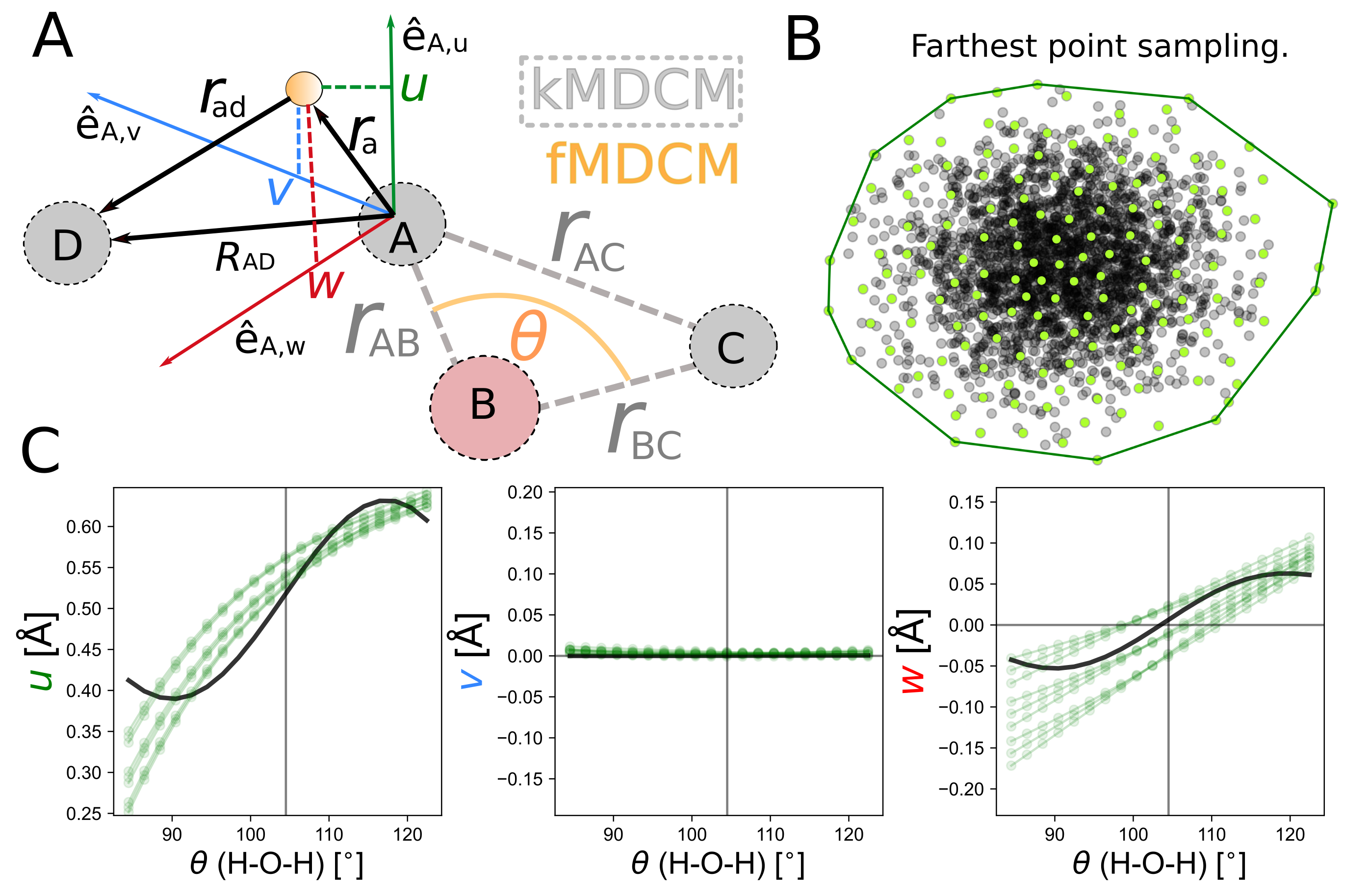
Figure 1: Panel A: Both fMDCM and kMDCM parametrize charge displacements (e.g. $r_{a}$ associated with atom A) along local axes $(u,v,w)$ using $(1-\cos{\theta}$) and internal distances $\mathbf{d}$, respectively. Panel B: An illustration of farthest-point sampling in 2D is shown, improving coverage of conformational space. Kernels create a convex support based on the distance between data points. Panel C: Comparison of the fitted local charge positions depending on $\theta$ for the kMDCM (green; multiple lines indicate different bond lengths) and fMDCM (black; $\theta-$dependent, polynomial-fitted charge displacements³³) for a single charge in a flexible six-charge water model. The vertical line is at the equilibrium angle $(\theta_{\rm e}=104.5^{\circ})$; the horizontal line indicates 0 Å in local coordinates, corresponding to atom-centered charges.

2.2 Kernel-Based MDCM derivatives

For MD simulations the derivatives of the interactions with respect to the Cartesian coordinates for each atom are required. As an example, the Coulomb interaction $V$ between charge $q_{\rm a,kMDCM}$ associated with site A (treated with kMDCM) and $q_{\rm d,PC}$ at site D (treated with atom-centered PC) is considered. Omitting the prefactor $(4\pi\varepsilon_{0})^{-1}$, the interaction is

$$V\propto\frac{q_{\rm a,kMDCM}\cdot q_{\rm d,PC}}{|\mathbf{r}_{\rm ad}|}$$ (12)

with $\mathbf{r}_{\rm ad}=\mathbf{R}_{\rm D}-(\mathbf{r}_{\rm a}+\mathbf{R}_{\rm A})$, see Figure 1, which may depend on some arbitrary molecular distortion $\mathbf{\rho}$, as described previously³³. With $\gamma=\{x,y,z\}$, the derivative of the corresponding Coulomb potential with respect to some change in position of atom A is

$$\frac{\partial V}{\partial R_{{\rm A},\gamma}}=q_{\rm a,kMDCM}\cdot q_{\rm d,PC}\frac{\partial}{\partial R_{{\rm A},\gamma}}\frac{1}{|{\mathbf{r}}_{\rm ad}|}$$ (13)

For any off-center, distributed charge (DC) model - such as MDCM, fMDCM or kMDCM - $\mathbf{r}_{\rm a}$ is defined relative to a local axis system $\hat{\bf e}_{{\rm A},x}$, $\hat{\bf e}_{{\rm A},y}$, $\hat{\bf e}_{{\rm A},z}$ defined by atoms A, B and C, as described elsewhere.²⁵ Forces on an off-center charge $q_{\rm a,DC}$ associated with atom A generate torques on atoms A, B and C according to Eq. (13) for these three atoms, replacing $\partial R_{\rm A}$ by $\partial R_{\rm B}$ or $\partial R_{\rm C}$ as appropriate. The complete set of partial derivatives for distributed charge $q_{\rm a,DC}$ is

$$\frac{\partial V}{\partial R_{{\rm A},\gamma}} =-\frac{q_{\rm a,DC}q_{\rm d,PC}\bigl{(}R_{{\rm AD},x}(\hat{\bm{\gamma}}\cdot\mathbf{\hat{x}}+g_{1\gamma})+R_{{\rm AD},y}(\hat{\bm{\gamma}}\cdot\mathbf{\hat{y}}+g_{2\gamma})+R_{{\rm AD},z}(\hat{\bm{\gamma}}\cdot\mathbf{\hat{z}}+g_{3\gamma})\bigr{)}}{|\bm{R}_{\rm AD}|^{3}}$$ (14)

$$\frac{\partial V}{\partial R_{{\rm B},\gamma}} =-\frac{q_{\rm a,DC}q_{\rm d,PC}\bigl{(}R_{{\rm AD},x}g_{4\gamma}+R_{{\rm AD},y}g_{5\gamma}+R_{{\rm AD},z}g_{6\gamma}\bigr{)}}{|\bm{R}_{\rm AD}|^{3}}$$ (15)

$$\frac{\partial V}{\partial R_{{\rm C},\gamma}} =-\frac{q_{\rm a,DC}q_{\rm d,PC}\bigl{(}R_{{\rm AD},x}g_{7\gamma}+R_{{\rm AD},y}g_{8\gamma}+R_{{\rm AD},z}g_{9\gamma}\bigr{)}}{|\bm{R}_{\rm AD}|^{3}}$$ (16)

where the scalar product $\hat{\bm{\gamma}}\cdot\mathbf{\hat{x}}$ is 1 for $\gamma=x$ and zero otherwise, $R_{{\rm AD},x}$ is the $x$-component of vector $\mathbf{R}_{\rm AD}$ pointing from atom A to D and the coefficients $g_{1\gamma}$ to $g_{9\gamma}$ contain the partial derivatives of the local unit vectors of the frame ($\mathbf{\hat{e}}_{u},\mathbf{\hat{e}}_{v},\mathbf{\hat{e}}_{w}$) with respect to the nuclear coordinate components $R_{{\rm A},\gamma}$, $R_{{\rm B},\gamma}$ and $R_{{\rm C},\gamma}$.²⁵

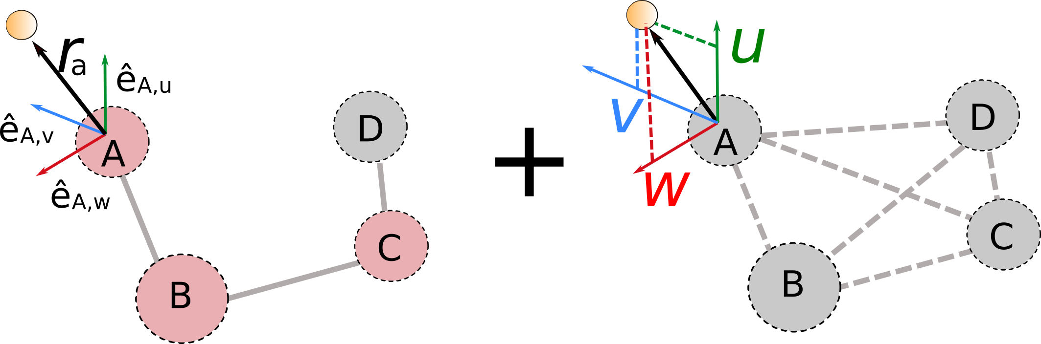
Figure 2: For an example tetra-atomic molecule, the charge displacement vector $\mathbf{r}_{a}$ depends on the local axes defined by the atoms (A,B,C), and the charge displacements along the local axes $u,v,w$. Eq. 17 defines the change in the $x$ component of $\mathbf{r}_{a}$ given displacement of atom $A$ in the $x$ direction.

Since $\kappa^{u}_{q}$, $\kappa^{v}_{q}$, and $\kappa^{w}_{q}$ depend on the interatomic distances vector $\mathbf{d}^{\prime}$, partial derivatives of the local unit vectors with respect to the nuclear coordinates contain contributions from each of the intermolecular distances involving atom A. As an example, the partial derivative $g_{1\gamma}(\mathbf{d^{\prime}})$ for the $x-$component of the Cartesian derivative of atom A is

$$g_{1\gamma}(\mathbf{d^{\prime}})= \Bigg{[}\kappa^{u}_{q}(\mathbf{d}^{\prime})\frac{\partial({\hat{\bf e}}_{{\rm A},u})_{x}}{\partial R_{{\rm A},\gamma}}+({\hat{\bf e}}_{{\rm A},u})_{x}\frac{\partial\kappa^{u}_{q}(\mathbf{d}^{\prime})}{\partial R_{{\rm A},\gamma}}\Bigg{]}+$$

$$\Bigg{[}\kappa^{v}_{q}(\mathbf{d}^{\prime})\frac{\partial({\hat{\bf e}}_{\rm A},v)_{x}}{\partial R_{{\rm A},\gamma}}+({\hat{\bf e}}_{{\rm A},v})_{x}\frac{\partial\kappa^{v}_{q}(\mathbf{d^{\prime}})}{\partial R_{{\rm A},\gamma}}\Bigg{]}+$$

$$\Bigg{[}\kappa^{w}_{q}(\mathbf{d}^{\prime})\frac{\partial({\hat{\bf e}}_{{\rm A},w})_{x}}{\partial R_{{\rm A},\gamma}}+({\hat{\bf e}}_{{\rm A},w})_{x}\frac{\partial\kappa^{w}_{q}(\mathbf{d^{\prime}})}{\partial R_{{\rm A},\gamma}}\Bigg{]}~{}.$$ (17)

Derivatives of the type $\partial\kappa^{u}_{q}(\mathbf{d}^{\prime})/\partial R_{{\rm A},\gamma}$ are evaluated using the chain rule, summing over all $N_{a}-1$ intramolecular distances with index $k$ including atom A to the remaining atoms X$\neq$A

$$\frac{\partial\kappa^{u}_{q}(\mathbf{d}^{\prime})}{\partial R_{{\rm A},\gamma}}=\sum^{N_{\mathrm{a}}-1}_{k=1}\frac{\partial\kappa^{u}_{q}(\mathbf{d}^{\prime})}{\partial d^{\prime}_{k}}\frac{\partial d^{\prime}_{k}}{\partial R_{{\rm A},\gamma}}$$ (18)

where

$$\frac{\partial\kappa^{u}_{q}(\mathbf{d}^{\prime})}{\partial d^{\prime}_{k}}= -\sum^{N_{\rm train}}_{i=1}\alpha_{i}K(\mathbf{d^{\prime},d}_{i})\frac{(d^{\prime}_{k}-d_{i,k})}{\sigma^{2}}$$ (19)

$$\frac{\partial d^{\prime}_{k}}{\partial R_{{\rm A},\gamma}}= \frac{R_{{\rm A},\gamma}-R_{{\rm X},\gamma}}{d_{k}}$$ (20)

and $d_{k}=|\mathbf{R}_{\rm A}-\mathbf{R}_{\rm X}|$ are internal distances involving atom A and X$\neq$A. This completes the derivation of analytical forces in Eq. 13.

As fMDCM also attempts to describe intramolecular charge redistribution, a model for water was constructed to compare directly with kMDCM presented in the present work. As an improvement over the earlier parametrization³³ which used a third order polynomial $\sum_{i=0}^{3}a_{i}\theta^{i}$ to describe the coordinate dependence of $(u(\theta),v(\theta),w(\theta))$, an expansion $\sum_{i=0}^{3}a_{i}(1-cos(\theta))^{i}$ was used in the following. This also improves the quality of the model when evaluated at angles close to 180^∘ which is particularly relevant for linear molecules such as SCN^-.⁴⁴.

2.3 Ab initio Reference Data

The molecular ESP, obtained from the converged SCF density at the PBE0/aug-cc-pVDZ level of theory was analysed using the CubeGen utility in Gaussian16⁴⁵ with a grid spacing of 1.67 points/Å. Water geometries were obtained by enumerating a $Z$-matrix representation on a 3-dimensional grid containing ten evenly spaced angles between $84.45^{\circ}$ to $120.45^{\circ}$, and each OH bond length sampled at 0.909 Å, 0.959 Å and 1.009 Å, resulting in 180 structures. For methanol, 2500 structures were sampled from gas phase MD simulations, using CHARMM⁴⁶ and CGenFF⁴ parameters, with bond lengths involving hydrogen atoms constrained using the SHAKE algorithm.⁴⁷ For generating methanol geometries, gas phase simulations were performed at 600 K using an integration time step $\Delta t=1$ fs. First, temperature was equilibrated using the Nosé-Hoover thermostat over 500 ps of simulation in the $NVT$ ensemble. 2.5 ns of simulation was then performed in the $NVE$ ensemble, with structures saved every 1 ps.

As with all machine learning-based methods, samples to train the model are required. Kernel models such as kMDCM use atom-atom distances within the input space as a basis for a prediction. As such, data coverage is an important consideration to ensure all relevant conformations are adequately described. Farthest-point sampling was used to select the conformations included in the training set to maximize the diversity of the structures used for training. This was achieved by randomly selecting an initial geometry and choosing each subsequent geometry by selecting the one with the largest Euclidean distance from the previous selection. An example of this procedure in 2D is illustrated in Figure 1B, where training examples at the boundary of the data distribution form the convex hull of the kernel.

2.4 MD Simulations using kMDCM

All molecular dynamics (MD) simulations were run using the CHARMM package.⁴⁶ Routines for calculating electrostatic energies and forces for kMDCM were implemented inside the DCM module.²⁶ To assess the validity and energy conservation of the kMDCM implementation, a periodic water box with a side length of 41 Å was set up containing 2000 water molecules. For the intramolecular potential of water, an RKHS³⁹ representation of reference energies at the PNO-LCCSD(T)/aug-cc-pVTZ level of theory was used.⁴⁸

For equilibration, the system was simulated in the $NpT$ ensemble at $T=300$ K and $p=1$ atm for 1 ns using $\Delta t=0.2$ fs with van der Waals parameters taken from CGenFF.⁴ Nonbonded interactions were truncated at 16 Å and electrostatic interactions were calculated using particle mesh Ewald summation. After equilibration the volume was kept constant during 500 ps of simulation in $NVT$, after which the thermostat was turned off and a further 1 ns of simulation in the $NVE$ ensemble was performed for data accumulation. Additionally, IR spectra were computed from the simulation data. The IR line shape, $I(\omega)$, was obtained via the Fourier transform of the dipole–dipole autocorrelation function from the dipole moment time series, with snapshots saved every 2 fs from a 500 ps $NVE-$simulation. For comparison, the anharmonic frequencies for a single gas phase water molecule calculated using DVR3D⁴⁹ for the bend, symmetric and asymmetric stretch were 1575, 3690, and 3719 cm^-1, respectively,⁴⁸ compared with experimentally observed frequencies⁵⁰ at 1595, 3657, and 3756 cm^-1 which validates the bonded terms.

3 Results

3.1 Quality of the ESP

First, methanol based on a 10 distributed charge model was selected as a test system to validate kMDCM and to assess the conformational dependence of the molecular ESP upon changes in angles and dihedrals. For this, 2500 methanol conformations were generated from a gas phase MD simulation initialized from velocities corresponding to a Maxwell-Boltzmann distribution at 300 K. For the kMDCM model 256 structures were used for training and the average RMSE for the test set was 1.0 kcal/(mol$\cdot e)$. When fitting to the remaining structures using conformational averaging, the RMSE was 1.2 kcal/(mol$\cdot e)$ for static MDCM, which increased to 2.0 kcal/(mol$\cdot e)$ for an atom-centered PC model, see Figure 3. Additionally, a dependence of the quality of the ESP on the COH angle was observed. Although averaging over an ensemble of structures is recommended^{15, 51, 52} this may lead to implicit bias in the quality of the models for certain conformations, as seen in Figure 3 (blue line). Distorted structures with COH angles $\theta\leq 100^{\circ}$ yielded smaller errors in comparison to more linear structures ($\theta\geq 160^{\circ}$) by approximately 0.2 kcal/(mol$\cdot e)$. The conformational dependence is less pronounced for PC models, likely due to the lower complexity of the fitting parameters and the higher baseline errors. The width of the error distribution of the new kMDCM model is smallest and no bias towards particular angles is observed.

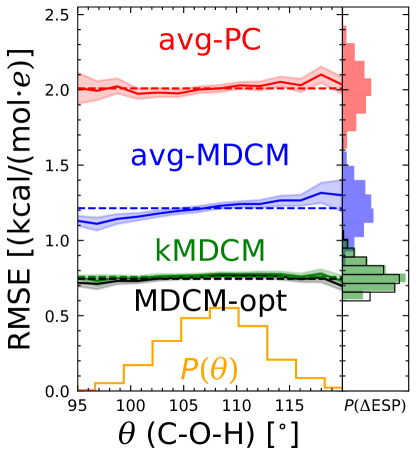
Figure 3: Left: The average ESP quality for methanol depending on the COH angle with static charge models avg-PC (red) and avg-MDCM (blue) compared with conformationally dependent kMDCM (green) and optimized positions using l-BFGS (black), evaluated on the test set. The shaded area shows the 99% confidence interval and the dashed horizontal lines indicate the position of the median RMSE. Right: the normalized distributions for $P(\Delta{\rm ESP}(\theta))$. The two static models exhibit conformational dependence w.r.t the COH angle. The distribution of angles is shown in orange.

Next, the performance of kMDCM for a water molecule was assessed by a systematic scan ($3\times 3\times 20=180$ structures for $r_{\mathrm{OH_{1}}}$, $r_{\mathrm{OH_{2}}}$, and $\theta_{\mathrm{H_{1}OH_{2}}}$) along both OH-bonds and the valence angle for water geometries. A 6 charge kMDCM model from farthest-point sampling using 16 structures was generated with an additional 164 structures available as the test set. The trained model achieved an average RMSE of 0.7 kcal/(mol$\cdot e)$ for the test set with a maximum error of 0.8 kcal/(mol$\cdot e)$. This compares with an average RMSE and maximum error of 0.7 kcal/(mol$\cdot e)$ and 1.1 kcal/(mol$\cdot e)$, respectively, for a fMDCM model fit to all structures. The favourable performance of the kMDCM and fMDCM models can be related to the fact that OH bond-coupling, which fMDCM is insensitive to, has less impact on the ESP changes than the variation of the valence angle. For the ensemble averaged MDCM, the water conformer with the highest RMSE was equal to 1.8 kcal/(mol$\cdot e)$, and was 1.0 kcal/(mol$\cdot e)$ on average for the entire distribution. In comparison, optimizing the ESP of a PC model to an average of all structures, gave an average RMSE of 2.3 kcal/(mol$\cdot e)$ and a maximum RMSE of 2.7 kcal/(mol$\cdot e)$. For water monomers with non-equilibrium bond lengths which incurred the highest errors, the improvement of $\sim 30\%$ for the RMSE between kMDCM and fMDCM shows the advantage of incorporating all conformational degrees of freedom into the kernel-based model. For both, fMDCM and kMDCM, the representation of $(u,v,w)$ depends in a similar fashion on the valance angle $\theta$, see Figure 1C. However, kMDCM which depends on all internal degrees of freedom captures this dependence in a more realistic fashion than fMDCM for which a third-order polynomial is not sufficiently flexible to describe the variation of $(u,v,w)$ with $\theta$ and does not depend on OH bond length.

3.2 Molecular Dipole Surface

The electrostatic models in this study were fit to reproduce the reference molecular ESP. However, modelling the conformational dependence of the molecular molecular dipole moment is equally important in computational spectroscopy as the intensity of IR transitions depend on it. To determine how the molecular dipole moment of methanol changes with conformation, simulations of a single methanol with constrained bonds involving hydrogen atoms were performed, and snapshots were taken every $0.1$ fs. The magnitude of the molecular dipole moment ${\mu}$ was computed for 2500 snapshots using the kMDCM and fMDCM models described above and compared with ab initio values calculated at the PBE0/aug-cc-pVDZ level of theory used for the reference calculations.

A direct comparison of the molecular dipole determined from different models for the ESP with the reference electronic structure calculations is given in Figure 4A. Depending on the conformation, the molecular dipole from reference PBE0 calculations $\mu_{\rm PBE0}$ varies between 1.5 and 2.0 D which demonstrates that the conformational dependence needs to be taken into account. The kMDCM model (green) yielded $\mu_{\rm kMDCM}$ with an RMSE of 0.04 D compared with $\mu_{\rm PBE0}$ and was effective at describing the conformationally dependent molecular dipole moment. This compares with RMSEs of $0.07$ D and $0.05$ D for $\mu_{\rm PC}$ and $\mu_{\rm MDCM}$ from conformationally independent PC and MDCM models (Figure 4A).

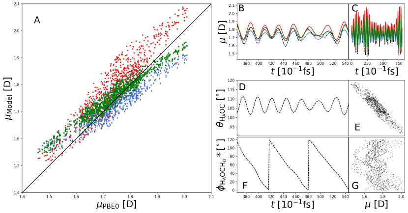
Figure 4: Performance of kMDCM, MDCM and PC models for methanol from MD-generated structures with constrained bonds involving hydrogen atoms. Panel A: The magnitude of the molecular dipole moment from DFT calculations $\mu_{\rm PBE0}$ versus $\mu_{\rm PC}$ (red), $\mu_{\rm MDCM}$ (blue), and $\mu_{\rm kMDCM}$ (green). Panels B and C: Model and reference (black dashed line) dipole moment time series $\mu(t)$ (zoom-in and full sequence); for color code see panel A. Panel D: Corresponding time series of the H_AOC angle. Panel E: Correlation between H_AOC angle and the reference $\mu_{\rm PBE0}$ Panel F: H_AOCH_B dihedral time series (^∗modulo 120 to account for the three fold symmetry of the rotation). Panel G: The reference dipole moment $\mu_{\rm PBE0}$ versus H_AOCH_B.

It is also interesting to consider the time-dependence of $\mu(t)$ (panels B and C) explicitly and to investigate whether its variation is correlated with particular internal motions, see panels D to G in Figure 4. The two coordinates considered were the H_AOC valence angle and the H_ACOH_B dihedral (where H_B are the methyl hydrogen atoms). Comparing panels D (angle) and E (dipole) clarifies that the variation of $\mu_{\rm PBE0}(t)$ correlates with changes in the valence angle whereas the dihedral motion does not correlate directly with the dipole moment, see panels F (dihedral) and G (dipole).

3.3 Impact of Model Parameters and Iterative Refinement

Besides the number of charges considered, a kMDCM model requires two hyperparameters to be chosen: $\lambda_{1}$ and $\lambda_{2}$. These may depend on the molecule considered and the purpose for which the model is developed. The impact of these hyperparameters is discussed for kMDCM models for water (6 charges each with $u$, $v$, $w$ to yield 18 kernels and 3 atom-atom separations) and for methanol (10 charges, 30 kernels, 15 atom-atom separations). As per the methods section, $\lambda_{1}$ adds a penalty to the loss function which increases with the displacement of charges with respect to their initial positions. For water, for which the loss landscape was found to be smoother compared with that for methanol, $\lambda_{1}=0$ kcal/(mol$\cdot e\cdot$Å) was found to be effective. On the other hand, for methanol, $\lambda_{1}=50$ kcal/(mol$\cdot e\cdot$Å) was used initially to prevent charges from moving too far and to better control and guide the optimization.

Figure 5: Correlation between optimized local displacement components ($u_{q}(d)$) and corresponding kernel predictions ($\kappa_{q}^{u}(d)$) for different values of the kernel regularization parameter ($\lambda_{2}$) for water (A1, B1) and methanol (C1, D1). Test and train examples are depicted as blue and orange circles, respectively. To the right, the accompanying distributions of $u_{q}(d)$ (black) and $\kappa_{q}^{u}(d)$ (yellow) the test set are shown (A2-D2).

$\lambda_{2}$	$\langle\mathrm{RMSE}\rangle^{\mathrm{dis.}}_{\mathrm{test}}$	$\langle\mathrm{RMSE}\rangle^{\mathrm{ESP}}_{\mathrm{test}}$	$\langle\mathrm{RMSE}\rangle^{\mathrm{dis.}}_{\mathrm{train}}$	$\langle\mathrm{RMSE}\rangle^{\mathrm{ESP}}_{\mathrm{train}}$
$10^{-8}$	0.006	0.60	0.000	0.62
$10^{-3}$	0.014	0.61	0.012	0.63
$10^{-1}$	0.036	0.75	0.038	0.79
$10^{0}$	0.078	0.96	0.084	1.03

Table 1: The average displacement between optimised and predicted charge positions ($\langle\mathrm{RMSE}\rangle^{\mathrm{dis.}}$) for the kMDCM model of water in units of Å. The average RMSE between ESPs of optimized and predicted charge positions ($\langle\mathrm{RMSE}\rangle^{\mathrm{ESP}}$) in kcal/(mol$\cdot e$).

$\lambda_{2}$	$\langle\mathrm{RMSE}\rangle^{\mathrm{dis.}}_{\mathrm{test}}$	$\langle\mathrm{RMSE}\rangle^{\mathrm{ESP}}_{\mathrm{test}}$	$\langle\mathrm{RMSE}\rangle^{\mathrm{dis.}}_{\mathrm{train}}$	$\langle\mathrm{RMSE}\rangle^{\mathrm{ESP}}_{\mathrm{train}}$
$10^{-8}$	0.004	1.07	0.000	1.07
$10^{-3}$	0.007	1.07	0.004	1.08
$10^{-1}$	0.016	1.11	0.016	1.11
$10^{0}$	0.023	1.15	0.026	1.15

Table 2: The average displacement between optimised and predicted charge positions ($\langle\mathrm{RMSE}\rangle^{\mathrm{dis.}}$) for the kMDCM model of methanol in units of Å. The average RMSE between ESPs of optimized and predicted charge positions ($\langle\mathrm{RMSE}\rangle^{\mathrm{ESP}}$) in kcal/(mol$\cdot e$).

Secondly, the kernel regularization parameter $\lambda_{2}$ weighs the trade-off between over- and under-fitting. For $\lambda_{2}=10^{-8}$ (Figure 5 A.1 and C.1) training examples (orange circles) are reproduced exactly. For water with only 3 degrees of freedom the test examples (blue circles) can be interpolated given the training examples, with $\langle{\rm RMSE}\rangle^{\mathrm{dis.}}_{\rm test}=0.006$ Å between the reference values $(u,v,w)$ after l-BFGS optimization and their representations ($\kappa_{q}^{u}$, $\kappa_{q}^{v}$, $\kappa_{q}^{w}$) with $\lambda_{2}=10^{-8}$. Furthermore, performance on the test set in terms of the average RMSE of the ESP across all conformers is lowest (Table 1). It is also noted that the range of the predictions increases for smaller values of $\lambda_{2}$ (Figure 5B.1, yellow histogram) compared with the reference values (black histogram). Conversely, for larger values of $\lambda_{2}$, the range of predicted values becomes smaller than that of the training examples (Figure 5 B.2 and D.2, yellow histograms), as $\lambda_{2}$ increases the effective cut-off distance to training examples in the input space causing predictions to be ‘averaged’ across more training structures. As a consequence, the distributions $P(\kappa^{u}_{q})$, $P(\kappa^{v}_{q})$, and $P(\kappa^{w}_{q})$ become more closely centered around the mean. For the high dimensional case, methanol, $\lambda_{2}=10^{-3}$ was found to achieve similar performance in the test set when compared to $\lambda_{2}=10^{-8}$; however, the average distance between ground-truth and predicted charge positions from 0.004 Å with low regularization to 0.007 Å  (Table 2).

Figure 6: Distributions of $\mathrm{RMSE}^{\mathrm{ESP}}_{\mathrm{test}}$ for l-BFGS optimized charge positions (red) versus kMDCM (black), for (A) no $\lambda_{1}$ penalty, and (B, C, D) iterative refinement after 1, 3, and 5 steps, respectively, using $\lambda_{1}=10$ kcal/(mol$\cdot e\cdot$Å). Insets show the correlation between the $u_{q}(d)$ and the kernel predictions, $\kappa_{q}^{u}(d)$. Kernels were fit with $\lambda_{2}=10^{-8}$.

To generate ensembles of charge positions that are amenable to interpolation using kMDCM, an iterative refinement scheme for fitting the kMDCMs was developed. Without adding a penalty the the charge displacements ($\lambda_{1}=0$ kcal/(mol$\cdot e\cdot$Å)) and starting from a conformationally averaged MDCM model for methanol, it was observed that the charge displacements were poorly interpolated (with $\lambda_{2}=10^{-8}$) using the kernel (Figure 6A, inset). The average and the range of $\mathrm{RMSE}^{\mathrm{ESP}}_{\mathrm{test}}$ was larger in comparison to the l-BFGS optimized models (Figure 6A), which may be related to the optimizer finding discontinuous local minima when no charge displacement penalty is applied, leading to inaccurate predictions. When a penalty of $\lambda_{1}=50$ kcal/(mol$\cdot e\cdot$Å) was used to restrict the displacement of the charges, the range of the charge displacements obtained by l-BFGS was small and reproduced accurately by the kernel 6B. This process was repeated by initializing the charge positions from the kernel prediction allowed the range of the predicted charge positions to increase in a controlled fashion, see Figure 6B-D. Following this iterative refinement lowered the RMSE for the test set while keeping the accuracy of the kernel’s predictions stable during the iterative refinement.

3.4 Molecular Dynamics Simulations with kMDCM

Next, the feasibility of meaningful MD simulations using kMDCM was assessed. This required that energy-conserving trajectories can be generated from simulations in the $NVE$ ensemble. For this, the formalism presented in the Methods section was implemented into the DCM module in CHARMM version c48. MD simulations were then run with 2000 water molecules in an equilibrated periodic box at 1 atm pressure without SHAKE constraints. The electrostatic model was a 6 charge kMDCM model, using Lennard-Jones parameters from the TIP3P water model⁵³ and the bonded terms were those of a RKHS representation,³⁹ see Methods section. As the electrostatic contribution of the force field was altered from the original parametrization, further refinement of non-bonded parameters will be necessary, e.g. along previously suggested lines,⁵⁴ for direct comparison of computed observables with experimentally measured properties. Such refinement was, however, not deemed necessary for validating the implementation and was not further pursued here.

Figure 7: (A) Fluctuations from the average total energy, $\Delta E(t)=E(t)-\langle E\rangle$, from an $NVE$ simulation of a 2000 molecule water box, using a time step of 0.2 fs. with kMDCM+RKHS. A running average over 200 ps is shown as a red, dashed line, (B) the corresponding distribution. (C) The simulated liquid phase IR spectrum in comparison with experiment⁵⁵. The intensity of the spectra was post-processed with a moving average over a sliding window of 15 cm^-1.

The combination of RKHS and kMDCM was found to be stable over the 1 ns long $NVE$ simulation, based on the variance in total energy over time and the corresponding distribution (Figures 7A and B). Simulations using kMDCM exhibit variances in the total energy of $\pm 0.5$ kcal/mol and $\pm 0.1$ kcal/mol for $\delta t=0.2$ fs and $\delta t=0.1$ fs, respectively. For reference, rigid TIP3P using SHAKE constraints leads to a variance in the total energy of $\pm 0.5$ kcal/mol using an integration time step of 1 fs.³³ As a test of the bonded terms, the simulated IR spectrum reproduces the low frequency features (Figure 7C). The frequency of the OH stretch vibrations are blue shifted in comparison with experiment which is known for high-frequency modes from MD simulations at 300 K.⁵⁶ Shifts in the low frequency modes may be related to the choice of non-bonded parameters, as the system had a density of 1.1 g/cm³ which is 10% larger than the experimental value. Improvements to the IR and other observables can be achieved through appropriate parametrization of the Lennard-Jones parameters which is outside the scope of the present work.

Figure 8: Input distance matrix values (top) for methanol, excluding SHAKEd bonds, and (bottom) output charge displacements versus saved simulation time step (0.001 ps between frames). Note that atom-charge distances are roughly one order of magnitude smaller than atom-atom distances. Red horizontal lines indicate coverage of the training set; black horizontal lines indicate the bounds of values obtained during simulation. (inset) A ball-and-stick structure of methanol with atom labels and distributed charges are shown. Positive and negative charges are colored blue and red, respectively.

It is also interesting to visualise the displacement dynamics of the distributed charges themselves. Kernel-based interpolation methods rely on establishing a convex hull of training examples to support their predictions. For equilibrium MD simulations, the extent of the conformational space needed to sample reliable structures may be large, depending on the size of the molecule and the active degrees of freedom. In the likely event that the molecule reaches a conformation that is not present in the training set, the dynamics of the distributed charges should be stable. Ensuring that the displacements of the distributed charges do not move too far away from the atom centers is important to prevent charges approaching too close to one another, causing extreme Coulomb interactions, or overstabilizing unphysical conformations.

The charge displacements during a gas phase methanol simulation are compared to the displacements present in the training set, for atom-atom distances, i.e. kernel input, which are mostly in the bounds of the training examples (Figure 8). The top panels show the intramolecular distances used as input to the kernel, where the red horizontal lines report the maximum and minimum values present in the training set. In the bottom panels, black horizontal lines indicate the bounds of the charge displacements sampled during the simulation. All charges remained within the bounds of the training distribution, with the exception of the fourth charge on the oxygen atom (O-q4, Figure 8) which moved slightly ($\sim 0.05$ Å) outside of the bounds but is still smaller than the $r_{\mathrm{min}}/2$ for the oxygen atom type of 1.79 Å in the CGenFF force field. All input distances remained inside the bounds of the training data, apart from the H1-H4 distance which reached a minimum distance at $\sim 440$ ps which was unseen by the kernel. Sharp drops in the displacements for some charges also occur at this time, as the similarity to training examples becomes lower, causing the kernel predictions to decay - although they remain within the bounds of the distribution.

4 Discussion and Conclusions

The present work introduces a kernel-based kMDCM to describe intramolecular charge redistribution and the conformational dependence of the molecular ESP in a fashion that is suitable for molecular (dynamics) simulations. As such, kMDCM is the full-dimensional generalization to explicitly parametrized flexible MDCM (fMDCM) where charge displacements $(u,v,w)$ depend, e.g., on a valence angle $\theta$.³³ In terms of performance, kMDCM improves the accuracy by a factor of two compared with a conformationally averaged PC-based model for methanol. To put this into perspective it should be mentioned that typical empirical force fields with fixed atom-centered PCs do not use conformationally averaged models^{4, 57, 58, 59} and improvements relative to such models are expected to be even larger. Similarly, for the molecular dipole moment a considerable conformational dependence was observed which can be best captured by kMDCM, followed by MDCM and PC models fit to ensembles of structures. However, it is notable that for the dipole moment (see Figure 4A) the PC-based model (red) overestimates the reference dipole moment from electronic structure calculations by a constant amount with a small tilt away from the diagonal towards higher values, whereas the two MDCM-based models overestimate small dipole moments and underestimate the largest values. It is also demonstrated here that meaningful and energy-conserving condensed-phase simulations for 2000 water molecules on the nanosecond time scale can be carried out. Thus, the present results provide a strong basis for the validity of kernel-based fluctuating charge models to systematically extend the scope of empirical force fields.

As with all machine learning-based methods, there are system parameters (hyperparameters) that are worthwhile to be analyzed in more detail. This showed, for example, that the expressivity of the model is largest for small values of $\lambda_{2}$ and increasing this hyperparameter ties the model more to the average data. In other words, $\lambda_{2}$ directly influences the smoothness of the model. This can also be characterized by the average norm of the Hessian^{60, 61} evaluated on off grid-points in Figure 9A. Small values of $\lambda_{2}$ cause charges to move more rapidly for conformations outside of the training set whereas larger values of $\lambda_{2}$ lead to more slowly-varying charge displacements without necessarily degrading the accuracy of the model in representing the conformational dependence of the ESP.

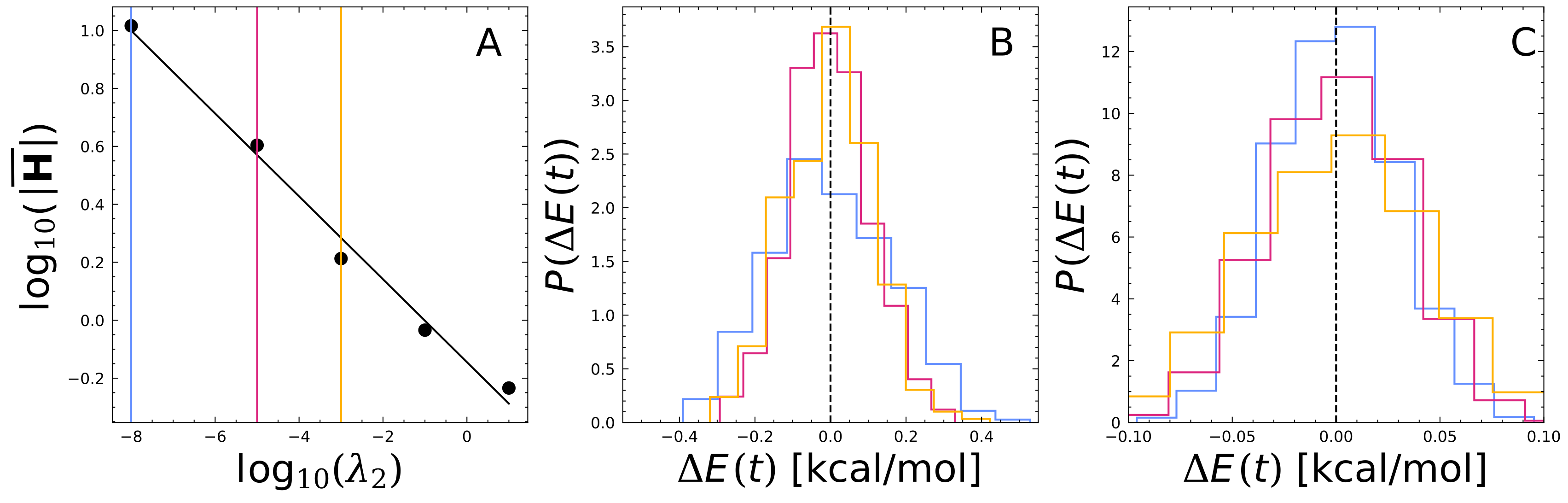
Figure 9: Panel A: The log-log relationship between the complexity parameter ($\lambda_{2}$) and the average norm of the Hessian (evaluated on off grid-points, for a single local charge position). kMDCM models fit using $\lambda_{2}$ of $10^{-8}$ (blue), $10^{-5}$ (red), $10^{-3}$ (orange) provide similar test set performance. Panels B and C: The distribution in the total energy fluctuations using a time step of 0.2 fs and 0.1 fs is largely insensitive to the choice of $\lambda_{2}$.

It is interesting to consider whether such effects impact the quality of MD simulations, e.g. with respect to conservation of the total energy in $NVE$ simulations. For this, models for water with $\lambda_{2}=10^{-8},10^{-5},10^{-3}$ were constructed. Three different time steps, $\Delta t=0.5,0.2,0.1$ fs, were used in the MD simulations. The distributions of the energy fluctuations around the mean are reported in Figures 9B and C for $\Delta t=0.2$ fs and 0.1 fs. The simulations were carried out for the water box with 2000 monomers, used the RKHS representation for intramolecular interactions and kMDCM for the electrostatics, with the bonds involving hydrogen atoms free to move (flexible monomers). The distributions $P(\Delta E)$ are largely insensitive to the value of $\lambda_{2}$ whereas doubling the time step from 0.1 to 0.2 fs causes the distribution to widen somewhat. For $\Delta t=0.5$ fs the simulations showed a monotonic increase in the total energy. Repeat simulations under the same conditions using PCs instead of kMDCM and the RKHS for the intramolecular contributions yielded comparable distributions and an increase in the total energy for $\Delta t=0.5$ fs which is due to the flexible OH-bonds. This was confirmed by running simulations with constrained OH bond lengths with $\Delta t=0.5$ and 1.0 fs using kMDCM which again conserved total energy. Hence, kMDCM allows robust, energy-conserving MD simulations.

The extrapolation capabilities of kMDCM were found to be satisfactory and suggest that the method can also be applied to larger and more flexible molecules, see Figure 5. Further improvement of the performance of kMDCM can be expected by changing the kernel functions from a Gaussian to other possible kernels.³⁹ Another extension is afforded by using the off-center PCs to describe external polarization. This will amount to evaluating kMDCM for a given structure and then reposition the off-center charges depending on the external electric field either in a self-consistent or a non-self-consistent manner.

In conclusion, kMDCM is a versatile model to describe intramolecular charge redistribution depending on molecular conformations. The formulation lends itself to be used in meaningful MD simulations and the approach was implemented in and validated with the CHARMM molecular simulation program.

Supporting Information Available

The codes for this work are available at https://github.com/MMunibas/kMDCM.

This work was supported by the Swiss National Science Foundation through grants $200020\_219779$ and $200021\_215088$ and the University of Basel, and by the European Union’s Horizon 2020 research and innovation program under the Marie Skłodowska-Curie grant agreement No 801459-FP-RESOMUS.

References

- Shim and MacKerell Jr 2011 Shim, J.; MacKerell Jr, A. D. Computational ligand-based rational design: role of conformational sampling and force fields in model development. MedChemComm 2011, 2, 356–370
- van Gunsteren et al. 2018 van Gunsteren, W. F.; Daura, X.; Hansen, N.; Mark, A. E.; Oostenbrink, C.; Riniker, S.; Smith, L. J. Validation of molecular simulation: an overview of issues. Angew. Chem. Int. Ed. 2018, 57, 884–902
- Töpfer et al. 2022 Töpfer, K.; Upadhyay, M.; Meuwly, M. Quantitative molecular simulations. Phys. Chem. Chem. Phys. 2022, 24, 12767–12786
- Vanommeslaeghe et al. 2010 Vanommeslaeghe, K.; Hatcher, E.; Acharya, C.; Kundu, S.; Zhong, S.; Shim, J.; Darian, E.; Guvench, O.; Lopes, P.; Vorobyov, I.; MacKerell, A. D. CHARMM General Force Field (CGenFF): A force field for drug-like molecules compatible with the CHARMM all-atom additive biological force fields. J. Comput. Chem. 2010, 31, 671–690
- Stone 2013 Stone, A. The theory of intermolecular forces; oUP oxford, 2013
- Rein 1973 Rein, R. Advances in quantum chemistry; Elsevier, 1973; Vol. 7; pp 335–396
- Cisneros et al. 2006 Cisneros, G. A.; Piquemal, J.-P.; Darden, T. A. Generalization of the Gaussian electrostatic model: Extension to arbitrary angular momentum, distributed multipoles, and speedup with reciprocal space methods. J. Chem. Phys. 2006, 125, 184101
- Plattner and Meuwly 2008 Plattner, N.; Meuwly, M. The role of higher CO-multipole moments in understanding the dynamics of photodissociated carbonmonoxide in myoglobin. Biophys. J. 2008, 94, 2505–2515
- Ponder et al. 2010 Ponder, J. W.; Wu, C.; Ren, P.; Pande, V. S.; Chodera, J. D.; Schnieders, M. J.; Haque, I.; Mobley, D. L.; Lambrecht, D. S.; DiStasio Jr, R. A., et al. Current status of the AMOEBA polarizable force field. J. Phys. Chem. B 2010, 114, 2549–2564
- Kramer et al. 2014 Kramer, C.; Spinn, A.; Liedl, K. R. Charge Anisotropy: Where Atomic Multipoles Matter Most. J. Chem. Theory Comput. 2014, 10, 4488–4496
- Jorgensen and Schyman 2012 Jorgensen, W. L.; Schyman, P. Treatment of halogen bonding in the OPLS-AA force field: application to potent anti-HIV agents. J. Chem. Theory Comput. 2012, 8, 3895–3901
- D’Avino et al. 2014 D’Avino, G.; Muccioli, L.; Zannoni, C.; Beljonne, D.; Soos, Z. G. Electronic polarization in organic crystals: a comparative study of induced dipoles and intramolecular charge redistribution schemes. J. Chem. Theory Comput. 2014, 10, 4959–4971
- Koch et al. 1995 Koch, U.; Popelier, P.; Stone, A. Conformational dependence of atomic multipole moments. Chem. Phys. Lett. 1995, 238, 253–260
- Faerman and Price 1990 Faerman, C. H.; Price, S. L. A transferable distributed multipole model for the electrostatic interactions of peptides and amides. J. Am. Chem. Soc. 1990, 112, 4915–4926
- Jensen 2022 Jensen, F. Using atomic charges to model molecular polarization. Phys. Chem. Chem. Phys. 2022, 24, 1926–1943
- Sedghamiz et al. 2017 Sedghamiz, E.; Nagy, B.; Jensen, F. Probing the Importance of Charge Flux in Force Field Modeling. J. Chem. Theory Comput. 2017, 13, 3715–3721
- Dinur 1990 Dinur, U. “Flexible” water molecules in external electrostatic potentials. J. Chem. Phys. 1990, 94, 5669–5671
- Maréchal 2011 Maréchal, Y. The molecular structure of liquid water delivered by absorption spectroscopy in the whole IR region completed with thermodynamics data. Journal of Molecular Structure 2011, 1004, 146–155
- Fanourgakis and Xantheas 2006 Fanourgakis, G. S.; Xantheas, S. S. The bend angle of water in ice Ih and liquid water: The significance of implementing the nonlinear monomer dipole moment surface in classical interaction potentials. The Journal of Chemical Physics 2006, 124, 174504
- Liu et al. 2020 Liu, C.; Piquemal, J.-P.; Ren, P. Implementation of Geometry-Dependent Charge Flux into the Polarizable AMOEBA+ Potential. J. Phys. Chem. Lett. 2020, 11, 419–426
- Bedrov et al. 2019 Bedrov, D.; Piquemal, J.-P.; Borodin, O.; MacKerell, A. D.; Roux, B.; Schröder, C. Molecular Dynamics Simulations of Ionic Liquids and Electrolytes Using Polarizable Force Fields. Chemical Reviews 2019, 119, 7940–7995
- Kim and Rhee 2019 Kim, S. S.; Rhee, Y. M. Modeling Charge Flux by Interpolating Atomic Partial Charges. Journal of Chemical Information and Modeling 2019, 59, 2837–2849
- Reynolds et al. 1992 Reynolds, C. A.; Essex, J. W.; Richards, W. G. Atomic charges for variable molecular conformations. J. Am. Chem. Soc. 1992, 114, 9075–9079
- Richter et al. 2022 Richter, W. E.; Duarte, L. J.; Bruns, R. E. Unavoidable failure of point charge descriptions of electronic density changes for out-of-plane distortions. Spectrochimica Acta Part A: Molecular and Biomolecular Spectroscopy 2022, 271, 120891
- Devereux et al. 2014 Devereux, M.; Raghunathan, S.; Fedorov, D. G.; Meuwly, M. A novel, computationally efficient multipolar model employing distributed charges for molecular dynamics simulations. J. Chem. Theory Comput. 2014, 10, 4229–4241
- Unke et al. 2017 Unke, O. T.; Devereux, M.; Meuwly, M. Minimal distributed charges: Multipolar quality at the cost of point charge electrostatics. J. Chem. Phys. 2017, 147, 161712
- Devereux et al. 2020 Devereux, M.; Pezzella, M.; Raghunathan, S.; Meuwly, M. Polarizable Multipolar Molecular Dynamics Using Distributed Point Charges. J. Chem. Theory Comput. 2020, 16, 7267–7280
- Liu et al. 2020 Liu, C.; Piquemal, J.-P.; Ren, P. Implementation of Geometry-Dependent Charge Flux into the Polarizable AMOEBA+ Potential. J. Phys. Chem. Lett. 2020, 11, 419–426
- Cools-Ceuppens et al. 2021 Cools-Ceuppens, M.; Dambre, J.; Verstraelen, T. Modeling electronic response properties with an explicit-electron machine learning potential. arXiv:2109.13111 [physics] 2021, arXiv: 2109.13111
- Zhu et al. 2023 Zhu, X.; Riera, M.; Bull-Vulpe, E. F.; Paesani, F. MB-pol(2023): Sub-chemical Accuracy for Water Simulations from the Gas to the Liquid Phase. J. Chem. Theory Comput. 2023, 19, 3551–3566
- Kramer et al. 2012 Kramer, C.; Gedeck, P.; Meuwly, M. Atomic multipoles: Electrostatic potential fit, local reference axis systems, and conformational dependence. J. Comput. Chem. 2012, 33, 1673–1688
- Oenen et al. 2024 Oenen, K.; Dinu, D. F.; Liedl, K. R. Determining internal coordinate sets for optimal representation of molecular vibration. The Journal of Chemical Physics 2024, 160, 014104
- Boittier et al. 2022 Boittier, E. D.; Devereux, M.; Meuwly, M. Molecular Dynamics with Conformationally Dependent, Distributed Charges. J. Chem. Theory Comput. 2022, 18, 7544–7554
- 34 Straatsma, T.; McCammon, J. Molecular dynamics simulations with interaction potentials including polarization development of a noniterative method and application to water. Mol. Sim. 5, 181–192
- Yu and van Gunsteren 2005 Yu, H.; van Gunsteren, W. F. Accounting for polarization in molecular simulation. Computer Physics Communications 2005, 172, 69–85
- Lopes et al. 2013 Lopes, P. E.; Huang, J.; Shim, J.; Luo, Y.; Li, H.; Roux, B.; MacKerell Jr, A. D. Polarizable force field for peptides and proteins based on the classical drude oscillator. J. Chem. Theory Comput. 2013, 9, 5430–5449
- Rasmussen and Williams 2006 Rasmussen, C. E.; Williams, C. K. I. Gaussian Processes for Machine Learning, www.GaussianProcess.org; MIT Press: Cambridge, 2006; Editor: T. Dietterich
- Ho and Rabitz 1996 Ho, T.-S.; Rabitz, H. A general method for constructing multidimensional molecular potential energy surfaces from ab initio calculations. J. Chem. Phys. 1996, 104, 2584–2597
- Unke and Meuwly 2017 Unke, O. T.; Meuwly, M. Toolkit for the Construction of Reproducing Kernel-Based Representations of Data: Application to Multidimensional Potential Energy Surfaces. J. Chem. Inf. Model. 2017, 57, 1923–1931
- Sauceda et al. 2019 Sauceda, H. E.; Chmiela, S.; Poltavsky, I.; Müller, K.-R.; Tkatchenko, A. Molecular force fields with gradient-domain machine learning: Construction and application to dynamics of small molecules with coupled cluster forces. J. Chem. Phys. 2019, 150
- Liu and Nocedal 1989 Liu, D. C.; Nocedal, J. On the limited memory BFGS method for large scale optimization. Mathematical Programming 1989, 45, 503–528
- Higham 2009 Higham, N. J. Cholesky factorization. WIREs Computational Statistics 2009, 1, 251–254
- Murphy 2012 Murphy, K. P. Machine Learning: A Probabilistic Perspective; The MIT Press, 2012; Chapter 14.4.3, pp 492–493
- Töpfer et al. 2022 Töpfer, K.; Pasti, A.; Das, A.; Salehi, S. M.; Vazquez-Salazar, L. I.; Rohrbach, D.; Feurer, T.; Hamm, P.; Meuwly, M. Structure, Organization, and Heterogeneity of Water-Containing Deep Eutectic Solvents. J. Am. Chem. Soc. 2022, 144, 14170–14180
- Frisch et al. 2016 Frisch, M. J. et al. Gaussian˜16 Revision C.01. 2016; Gaussian Inc. Wallingford CT
- Brooks et al. 1983 Brooks, B. R.; Bruccoleri, R. E.; Olafson, B. D.; States, D. J.; Swaminathan, S.; Karplus, M. CHARMM: a program for macromolecular energy, minimization and dynamics calculations. J. Comput. Chem. 1983, 4, 187–217
- Ryckaert et al. 1977 Ryckaert, J.-P.; Ciccotti, G.; Berendsen, H. J. C. Numerical integration of the cartesian equations of motion of a system with constraints: molecular dynamics of n-alkanes. J. Chem. Phys. 1977, 23, 327–341
- L. Fischer et al. 2023 L. Fischer, T. et al. The first HyDRA challenge for computational vibrational spectroscopy. Phys. Chem. Chem. Phys. 2023, 25, 22089–22102
- Tennyson et al. 2004 Tennyson, J.; Kostin, M. A.; Barletta, P.; Harris, G. J.; Polyansky, O. L.; Ramanlal, J.; Zobov, N. F. DVR3D: a program suite for the calculation of rotation–vibration spectra of triatomic molecules. Comput. Phys. Commun. 2004, 163, 85–116
- Shimanouchi 1972 Shimanouchi, T. Tables of Molecular Vibrational Frequencies, Consolidated Volume; National Bureau of Standards: Washington, 1972
- Sedghamiz et al. 2017 Sedghamiz, E.; Nagy, B.; Jensen, F. Probing the Importance of Charge Flux in Force Field Modeling. Journal of Chemical Theory and Computation 2017, 13, 3715–3721
- Koch et al. 1995 Koch, U.; Popelier, P. L. A.; Stone, A. J. Conformational dependence of atomic multipole moments. Chem. Phys. Lett. 1995, 238, 253–260
- Jorgensen et al. 1983 Jorgensen, W. L.; Chandrasekhar, J.; Madura, J. D.; Impey, R. W.; Klein, M. L. Comparison of simple potential functions for simulating liquid water. The Journal of Chemical Physics 1983, 79, 926–935
- Devereux et al. 2024 Devereux, M.; Boittier, E. D.; Meuwly, M. Systematic improvement of empirical energy functions in the era of machine learning. J. Comput. Chem. 2024, in print, in print
- Max and Chapados 2009 Max, J.-J.; Chapados, C. Isotope effects in liquid water by infrared spectroscopy. III. H2O and D2O spectra from 6000 to 0 cm-1. J. Chem. Phys. 2009, 131, 184505
- Nejad and Suhm 2020 Nejad, A.; Suhm, M. A. Concerted pair motion due to double hydrogen bonding: The formic acid dimer case. J. Indian Inst. Sci. 2020, 100, 5–19
- Jorgensen et al. 1996 Jorgensen, W. L.; Maxwell, D. S.; Tirado-Rives, J. Development and testing of the OPLS all-atom force field on conformational energetics and properties of organic liquids. J. Am. Chem. Soc. 1996, 118, 11225–11236
- Oostenbrink et al. 2005 Oostenbrink, C.; Soares, T. A.; Van Der Vegt, N. F.; Van Gunsteren, W. F. Validation of the 53A6 GROMOS force field. Eur. Biophys. J. 2005, 34, 273–284
- Wang et al. 2004 Wang, J.; Wolf, R. M.; Caldwell, J. W.; Kollman, P. A.; Case, D. A. Development and testing of a general amber force field. J. Comput. Chem. 2004, 25, 1157–1174
- Colesanti and Hug 2005 Colesanti, A.; Hug, D. Hessian Measures of Convex Functions and Applications to Area Measures. J. London Math. Soc. 2005, 71, 221–235
- Duchamp and Stuetzle 2003 Duchamp, T.; Stuetzle, W. Spline Smoothing on Surfaces. J. Comput. and Graph. Stat. 2003, 12, 354–381