Analysis of three-body decays $B\to D(V\to)PP$ under the factorization-assisted topological-amplitude approach

Abstract

Motived by the accumulated experimental results on three-body charmed $B$ decays with resonance contributions in Babar, LHCb and Belle (II), we systematically analyze $B_{(s)}\to D_{(s)}(V\to)P_{1}P_{2}$ decays with $V$ representing a vector resonance ($\rho,K^{*},\omega$ or $\phi$) and $P_{1,2}$ as a light pseudoscalar meson (pion or kaon). The intermediate subprocesses $B_{(s)}\to D_{(s)}V$ are calculated with the factorization-assisted topological-amplitude (FAT) approach and the intermediate resonant states $V$ described by the relativistic Breit-Wigner distribution successively decay to $P_{1}P_{2}$ via strong interaction. Taking all lowest resonance states ($\rho,K^{*},\omega,\phi$) into account, we calculate the branching fractions of these decay modes as well as the Breit-Wigner-tail effects for $B_{(s)}\to D_{(s)}(\rho,\omega\to)KK$. Our results agree with the data by Babar, LHCb and Belle (II). Among the predictions that are still not observed, there are some branching ratios of order $10^{-6}-10^{-4}$ which are hopeful to be measured by LHCb and Belle II. Our approach and the perturbative QCD approach (PQCD) adopt the compatible theme to deal with the resonance contributions. What’s more, our data for the intermediate two-body charmed $B$-meson decays in FAT approach are more precise. As a result, our results for branching fractions have smaller uncertainties, especially for color-suppressed emission diagram dominated modes.

I Introduction

Three-body nonleptonic $B$ meson decays not only are important for the study of common topics of nonleptonic $B$ meson decays, such as testing the standard model (SM), the studying the mechanism of $CP$ violation and the emergence of quantum chromodynamics, but also provide opportunities for the analysis on the hadron spectroscopy. Specifically, three-body $B$ meson decays have nontrivial kinematics and phase space distributions, which are usually described in terms of three two-body invariant mass squared combinations and two of them constitute two axes to form a Dalitz plot. In the edges of the Dalitz plot, the invariant mass squared combinations of two final-state particles will generally peak as resonances, which indicates that intermediate resonances in three-body $B$ meson decays show up, and we are able to study the properties of these resonances through three-body $B$ meson decays.

The Dalitz plot technique has proven to be a powerful tool to analyze the hadron spectroscopy and is widely adopted by experiments. The informations on various resonance substructures including the mass, spin-parity quantum numbers, etc. have been collected by Babar, Belle (II) and LHCb Belle:2006wbx ; BaBar:2009pnd ; BaBar:2010rll ; LHCb:2014ioa ; LHCb:2015klp ; LHCb:2015tsv ; LHCb:2018oeb ; Belle-II:2023gye . Simultaneously, usually under the framework of isobar model PhysRevD.11.3165 , these collaborations have also measured fit fractions of each resonance and nonresonance components. In the isobar model, the total decay amplitude can be expressed as a coherent sum of amplitudes of different resonant and nonresonant intermediate processes, where the relativistic Breit-Wigner (RBW) model usually describe resonant dynamics and exponential distribution for nonresonant terms. It is a very good approximation to adopt the RBW function for narrow width resonances which can be well separated from any other resonant or nonresonant components in the same partial wave, so that the three-body decays with narrow intermediate states, such as $\rho,K^{*},\omega,\phi$, have been precisely measured by experiments BaBar:2009pnd ; BaBar:2010rll ; LHCb:2011yev ; LHCb:2014ioa ; BaBar:2015pwa ; LHCb:2015klp ; LHCb:2015tsv ; LHCb:2018oeb ; LHCb:2019sus .

On the theoretical side, analysis on the nonresonant contributions of three-body $B$ meson decays are in an early stage of development. Approaches or models such as the heavy meson chiral perturbation theory Cheng:2002qu ; Cheng:2007si ; Cheng:2013dua and a model combing the heavy quark effective theory and chiral Lagrangian Fajfer:2004cx have been applied for calculating the nonresonant fraction of three-body charmless $B$ meson decays, such as $B\to KKK,\,B\to K\pi\pi$ which are dominated by nonresonant contribution Cheng:2008vy . More theoretical interest is concentrated on the resonant component of three-body $B$ decays, where two of the three final particles are produced from a resonance and recoil against the third meson called a “bachelor” meson. This type of three-body decay is also called quasi-two-body decay. Because of the large energy release in $B$ meson decays, the two meson pair moves fast antiparrallelly to the bachelor meson in the $B$ meson rest frame. Therefore, the interactions between the meson pair and the bachelor particle are power suppressed naturally which is similar to the statement of “color transparency” in two-body $B$ meson decays. Then approaches based on the factorization hypothesis have been proposed for calculating the quasi-two-body decays, such as the QCD Factorization (QCDF) Cheng:2002qu ; Cheng:2007si ; Cheng:2013dua ; Huber:2020pqb , the PQCD approachChen:2002th ; Wang:2014ira ; Wang:2016rlo ; Li:2016tpn ; Li:2018psm ; Wang:2020plx ; Fan:2020gvr ; Wang:2020nel ; Zou:2020atb ; Zou:2020fax ; Zou:2020ool ; Yang:2021zcx ; Liu:2021sdw ; Zhang:2022pfn ; Zhang:2023uoy ; Zhao:2023dnz ; Chang:2024qxl and factorization-assisted topological-amplitude (FAT) approach Zhou:2021yys ; Zhou:2023lbc .

In this work, we focus on three-body charmed $B$ decays $B_{(s)}\to D_{(s)}P_{1}P_{2}$, where $P_{1,2}$ represents a pion or kaon. Different from charmless decays, intermediate resonances in $B_{(s)}\to D_{(s)}P_{1}P_{2}$ decays are expected to appear in the $m^{2}(DP_{1})$ and $m^{2}(P_{1}P_{2})$ combinations, thus more resonances, such as charmed states $D^{*}$ and light vector or scalar resonances, can be researched simultaneously in one Dalitz plot. In addition, they provide opportunities for studies of CP violations. In particular, the Dalitz plot analysis of $B^{0}\to DK^{+}\pi^{-}$ can be used as a channel to measure the unitarity triangle angle $\gamma$ Gershon:2008pe ; Gershon:2009qc and $B^{0}\to\bar{D}^{0}\pi^{+}\pi^{-}$ is sensitive to the $\beta$ angle BaBar:2007fxn ; Belle:2006wor . Therefore, much attention has been already paid to $B_{(s)}\to D_{(s)}P_{1}P_{2}$ decays in experiments and theoretical calculations. LHCb Collaborations have investigated structures of ground and excited states of $D^{*}$, $K^{*}$ with their corresponding fit fractions through $B_{(s)}\to D_{(s)}K\pi$ LHCb:2011yev ; LHCb:2014ioa , and $D^{*}$, $\rho$ in $B_{(s)}\to D_{(s)}\pi\pi$ by Babar and Belle Belle:2006wbx ; BaBar:2010rll . Recently, the virtual contribution from $\rho$ in $B_{(s)}\to D_{(s)}KK$ has been measured by Belle II Belle-II:2023gye . Motived by the experimental progress on $B_{(s)}\to D_{(s)}P_{1}P_{2}$ decays, theoretical calculation on the branching fractions of various types of charmed quasi-two-body decays, $B_{(s)}\to D_{(s)}\pi\pi$, $B_{(s)}\to D_{(s)}K\pi$ and $B_{(s)}\to D_{(s)}KK$ with intermediate resonances $D^{*}$, $\rho,K^{*},\phi$ have been completed in a series of works with the PQCD approach Ma:2016csn ; Ma:2020dvr ; Chai:2021kie ; Zou:2022xrr ; Fang:2023dcy ; Wang:2024enc . In FAT approach, we have done a systematic research on $B_{(s)}\to D_{(s)}P_{1}P_{2}$ with ground charmed mesons $D^{*}$ as the intermediate states and $P_{1},P_{2}$ representing $\pi$ or $K$ Zhou:2021yys . The results of $B\to D^{*}P_{2}\to DP_{1}P_{2}$ in FAT approach are in better agreement with experimental data and more precise than the PQCD approach’s predictions.

FAT approach is firstly proposed to resolve the problem about nonfactorizable contributions in two-body $D$ and $B$ meson decays Li:2012cfa ; Li:2013xsa ; Zhou:2015jba ; Zhou:2016jkv ; Jiang:2017zwr ; Zhou:2019crd ; Zhou:2021yys ; Qin:2021tve and then has been successfully generalized to quasi-two-body $B$ meson decays Zhou:2021yys ; Zhou:2023lbc . It is based on the framework of conventional topological diagram approach, which is used to classify the decay amplitudes by different electroweak Feynman diagrams, but keeping $SU(3)$ breaking effects. Only a few unknown nonfactorization parameters need to be fitted globally with all experimental data. Therefore, FAT approach is able to provide the most precise decay amplitudes of (intermediate) two-body $B$ meson decays especially with charmed meson final states. Then in a quasi-two-body $B$ meson decay the intermediate resonances successively decay to final meson pairs via strong interaction, which are described in terms of the usual RBW formalism as what’s done in experiments. Actually, in the PQCD approach the light cone distribution amplitude (LCDA) of a meson pair originating from a P-wave resonance can be expressed as time-like form factors and then is also parameterized by the RBW distribution. So their framework of dealing with the resonances is compatible with that in FAT. More details about this can be found in Wang:2024enc . Therefore, the main difference between the FAT and the PQCD approach in quasi-two-body decays is how to calculate the intermediate two-body weak decays. It is well known that large nonperturbative contributions and power corrections expanded in $m_{c}/m_{b}$ of color suppressed and W-exchange diagrams in charmed $B$ decays have not been able to be calculated in PQCD approach Keum:2003js , which results in large uncertainties of PQCD approach’s predictions for $B\to DP_{1}P_{2}$ with resonances $D^{*}$, $\rho,K^{*},\phi$. In this paper we will apply FAT approach to study the $B_{(s)}\to D_{(s)}P_{1}P_{2}$ decay with the ground state light vector intermediate resonances $\rho,K^{*},\phi,\omega$, which are generally the largest components and their fit fractions have been well measured separately from any other vector resonances in LHCb and Belle II Belle:2006wbx ; LHCb:2014ioa ; LHCb:2015klp ; LHCb:2015tsv ; LHCb:2018oeb ; Belle-II:2023gye .

This paper is organized as follows. In Sec. II, the theoretical framework is introduced. The numerical results and discussions about $B_{(s)}\to D_{(s)}(\rho\to)\pi\pi$, $B_{(s)}\to D_{(s)}(K^{*}\to)K\pi$, $B_{(s)}\to D_{(s)}(\phi\to)K\bar{K}$ and $B_{(s)}\to D_{(s)}(\rho,\omega\to)K\bar{K}$ are collected in Sec. III. Finally, a summary is given in Section IV .

II FACTORIZATION OF AMPLITUDES FOR TOPOLOGICAL DIAGRAMS

The charmed quasi-two-body decay $B_{(s)}\to D_{(s)}(V\to)P_{1}P_{2}$ happens through two subprocesses, where the $D_{(s)}$ meson represents $D_{(s)}$ or its antiparticle $\bar{D}_{(s)}$. $B_{(s)}$ meson decays to an intermediate resonant state $D_{(s)}V$ firstly, and subsequently the unstable resonance decays to a pair of light psudoscaler, $V\to P_{1}P_{2}$. The first subprocess at quark level is induced by weak transitions $b\rightarrow\,c\,q\,\bar{u}\,\,(q=d,s)$ and $b\rightarrow\,u\,q\,\bar{c}\,\,(q=d,s)$ for $D_{(s)}$ and $\bar{D}_{(s)}$ final states, respectively. The secondary one proceeds directly by strong interaction. According to the topological structures of $b\rightarrow\,c\,q\,\bar{u}$, the diagrams contributing to $\bar{B}_{(s)}\to D_{(s)}(V\to)P_{1}P_{2}$ can be classified into three types as listed in Fig. 1, a) color-favored emission diagram $T$, b) color-suppressed emission diagram $C$, and c) $W$-exchange diagram $E$.

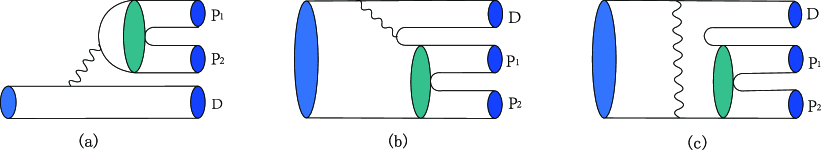
Figure 1: Topological diagrams of $\bar{B}_{(s)}\to D_{(s)}(V\to)P_{1}P_{2}$ under the framework of quasi-two-body decay with the wave line representing a $W$ boson: (a) the color-favored emission diagram $T$, (b) the color-suppressed emission diagram $C$, and (c) the W-exchange diagram $E$.

Similarly, besides $T,\,C,\,E$ diagrams, the topologies of $\bar{B}_{(s)}\to\bar{D}_{(s)}(V\to)P_{1}P_{2}$ induced by $b\rightarrow\,u\,q\,\bar{c}$ transitions include an additional W-annihilation diagram $A$ as shown in Fig. 2.

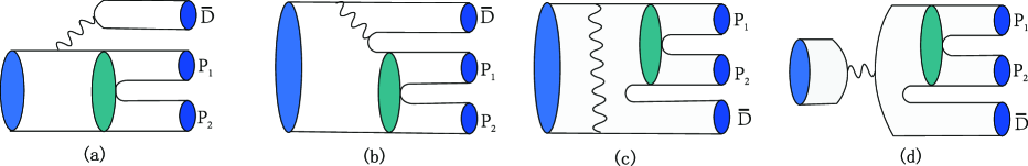
Figure 2: Topological diagrams of $\bar{B}_{(s)}\to\bar{D}_{(s)}(V\to)P_{1}P_{2}$ under the framework of quasi-two-body decay with the wave line representing a $W$ boson: (a) the color-favored emission diagram $T$, (b) the color-suppressed emission diagram $C$, (c) the W-exchange diagram $E$, and (d) W-annihilation diagram $A$.

The amplitudes of the first subprocess $\bar{B}_{(s)}\to D_{(s)}V$ can be refered to the ones of two-body charmed $B$ decays in FAT approach Zhou:2015jba . Factorization has been proven in $T$ topology at high precision. However, large nonfactorizable contributions have been found in $C$ and $E$. As done in Zhou:2015jba , we parameterize matrix elements of the nonfactorizable diagrams $C$ and $E$ in FAT approach and a well proven factorization formula for $T$, which can be expressed as follows,

$$\begin{aligned} T^{DV}&=\sqrt{2}\,G_{F}\,V_{cb}V_{uq}^{*}\,a_{1}(\mu)\,f_{V}\,m_{V}\,F_{1}^{B\rightarrow D}\left(m_{V}^{2}\right)\left(\varepsilon_{V}^{*}\cdot p_{B}\right),\\ C^{DV}&=\sqrt{2}\,G_{F}\,V_{cb}V_{uq}^{*}\,f_{D_{(s)}}\,m_{V}\,A_{0}^{B\rightarrow V}\left(m_{D}^{2}\right)\left(\varepsilon_{V}^{*}\cdot p_{B}\right)\,\chi^{C}\,e^{i\phi^{C}},\\ E^{DV}&=\sqrt{2}\,G_{F}\,V_{cb}V_{uq}^{*}\,m_{V}\,f_{B}\,\frac{f_{D_{(s)}}f_{V}}{f_{D}f_{\pi}}\,\left(\varepsilon_{V}^{*}\cdot p_{B}\right)\,\chi^{E}e^{i\phi^{E}}\,.\end{aligned}$$ (1)

So far there is not enough experimental data to do a global fit for $\bar{B}_{(s)}\to\bar{D}_{(s)}V$ decays to extract the unknown nonfactorizable parameters in the $C,E$ amplitudes. Therefore, the same nonfactorizable parameters $\chi^{C},\,\phi^{C},\,\chi^{E},\,\phi^{E}$ as those for $\bar{B}_{(s)}\to D_{(s)}V$ are adopted in a good approximation, just as what we do in Ref. Zhou:2015jba . The topological diagram $A$ for $\bar{B}_{(s)}\to\bar{D}_{(s)}V$ is dominated by large factorizable contribution and can be calculated in the pole model Zhou:2015jba , which is given as

$$\begin{aligned} A^{\bar{D}V}&=-\sqrt{2}\,G_{F}\,V_{ub}V_{cq}^{*}\,a_{1}(\mu)\,f_{B}\,\frac{f_{D_{(s)}}g_{DDV}m_{D}^{2}}{m_{B}^{2}-m_{D}^{2}}(\varepsilon^{*}_{V}\cdot p_{B})\,.\end{aligned}$$ (2)

For simplification of notations, we omit the subscript ‘(s)’ in $D_{(s)}$ in eqs. (1,2) and the following equations except in $f_{D_{(s)}}$. $a_{1}({\mu})$ is the effective Wilson coefficient for the factorizable topologies $T$ and $A$. $\chi^{C(E)}$ and $\phi^{C(E)}$ represent the magnitude and associated phase of $C$($E$) diagram globally fitted with the experimental data. $f_{V}$, $f_{D_{(s)}}$ and $f_{B}$ are the decay constants of the corresponding vector, $D_{(s)}$ and $B$ mesons. $F_{1}^{B\to D}$ and $A_{0}^{B\to V}$ denote the vector form factors of $B_{(s)}\to D$ and $B_{(s)}\to V$ transitions, which depend on the square of transfer momentum $Q^{2}$ and can be parameterized in pole model as,

$$F_{i}(Q^{2})={F_{i}(0)\over 1-\alpha_{1}{Q^{2}\over m_{\rm pole}^{2}}+\alpha_{2}{Q^{4}\over m_{\rm pole}^{4}}},$$ (3)

where $F_{i}$ represents $F_{1}$ or $A_{0}$, and $m_{\rm pole}$ is the mass of the corresponding pole state, such as $B^{*}$ for $F_{1}$ and $B$ for $A_{0}$. $\alpha_{1,2}$ are the model parameters. In eq.(2), $g_{DDV}$ is the effective strong coupling constant and its value can be obtained from the vector meson dominance model PhysRevC.62.034903 , $g_{DDV}=2.52$.

Next we will illustrate the calculation of the second subprocess, e.g. intermediate resonances decay to final states via strong interaction, $V\to P_{1}P_{2}$. As what’s done in experiments BaBar:2011vfx ; BaBar:2012bdw ; LHCb:2019sus , we also adopt the RBW distribution for $\rho$,  $K^{*}$,  $\omega$, and $\phi$ resonances, which is expressed as Cheng:2013dua ,

$$L^{\mathrm{RBW}}(s)=\frac{1}{s-m_{V}^{2}+im_{V}\Gamma_{V}(s)}\,,$$ (4)

where $s$ represents the invariant mass square of meson pair with 4-momenta $p_{1},\,p_{2}$, $s=(p_{1}+p_{2})^{2}$. $\Gamma_{V}(s)$ represents $s$-dependent width of vector resonances and is defined as

$$\Gamma_{V}(s)=\Gamma_{0}\left(\frac{q}{q_{0}}\right)^{3}\left(\frac{m_{V}}{\sqrt{s}}\right)X^{2}\left(q\,r_{\mathrm{BW}}\right)\,,$$ (5)

where $X(q\,r_{\mathrm{BW}})$ is the Blatt-Weisskopf barrier factor,

$$X\left(q\,r_{\mathrm{BW}}\right)=\sqrt{[1+\left(q_{0}\,r_{\mathrm{BW}}\right)^{2}]/[1+\left(q\,r_{\mathrm{BW}}\right)^{2}}]\,.$$ (6)

In the above two equations, $q=\frac{1}{2}\sqrt{\left[s-\left(m_{P_{1}}+m_{P_{2}}\right)^{2}\right]\left[s-\left(m_{P_{1}}-m_{P_{2}}\right)^{2}\right]/s}$ is momentum magnitude of the final state $P_{1}$ or $P_{2}$ in the rest frame of resonance $V$, and $q_{0}$ is just value of $q$ when intermediate resonance is on-shell, $s=m^{2}_{V}$. While for the case that the pole mass locates outside the kinematics region, i.e., $m_{V}<m_{P_{1}}+m_{P_{2}}$, $m_{V}$ needs to be replaced by an effective mass $m^{\mathrm{eff}}_{V}$ so that $\sqrt{s}=m^{\mathrm{eff}}_{V}$ for $q_{0}$. The effective mass $m^{\mathrm{eff}}_{V}$ is given by the ad hoc formula Aaij:2014baa ; Aaij:2016fma ,

$$m_{V}^{\text{eff }}\left(m_{V}\right)=m^{\min}+\left(m^{\max}-m^{\min}\right)\left[1+\tanh\left(\frac{m_{V}-\frac{m^{\min}+m^{\max}}{2}}{m^{\max}-m^{\min}}\right)\right]\,,$$ (7)

where $m^{\max}$ ($m^{\min}$) is the upper (lower) boundary of the kinematics region. Another parameter together with $q$ in $X(q\,r_{\mathrm{BW}})$ is the the barrier radius with its value $r_{\mathrm{BW}}=4.0(\mathrm{GeV})^{-1}$ for all resonances LHCb:2019sus . $\Gamma_{0}$ in eq.(5) represents the full widths of the resonant states and their values are taken from Particle Data Group (PDG) Workman:2022ynf and listed in Table 1 together with their masses $m_{V}$.

Table 1: Masses $m_{V}$ and full widths $\Gamma_{0}$ of vector resonant states.Workman:2022ynf

Resonance	Line shape Parameters	Resonance	Line shape Parameters
$\rho(770)~{}~{}$	$m_{V}\,=\,775.26\,\,\mathrm{MeV}$	$\omega(782)~{}~{}$	$m_{V}\,=\,782.65\,\,\mathrm{MeV}$
	$\Gamma_{0}\,=\,149.1\,\,\mathrm{MeV}$		$\Gamma_{0}\,=\,8.49\,\,\mathrm{MeV}$
$K^{*}(892)^{+}~{}~{}$	$m_{V}\,=\,891.66\,\,\mathrm{MeV}$	$K^{*}(892)^{0}~{}~{}$	$m_{V}\,=\,895.55\,\,\mathrm{MeV}$
	$\Gamma_{0}\,=\,50.8\,\,\mathrm{MeV}$		$\Gamma_{0}\,=\,47.3\,\,\mathrm{MeV}$
$\phi(1020)~{}~{}$	$m_{V}\,=\,1019.46\,\,\mathrm{MeV}$
	$\Gamma_{0}\,=\,4.25\,\,\mathrm{MeV}$

After getting the distribution function of the vector resonances, we proceed to consider matrix element $\left\langle P_{2}\left(p_{2}\right)P_{3}\left(p_{3}\right)|V(p_{V})\right\rangle$. It can be parametrized as a strong coupling constant $g_{VP_{1}P_{2}}$ which describes the strong interactions of the three mesons at hadron level. Inversely, the strong coupling constant $g_{VP_{1}P_{2}}$ can be extracted from the partial decay widths $\Gamma_{V\to P_{1}P_{2}}$ by

$$\Gamma_{V\rightarrow P_{1}P_{2}}=\frac{2}{3}\frac{p_{c}^{3}}{4\pi m_{V}^{2}}g_{VP_{1}P_{2}}^{2}\,,$$ (8)

where $p_{c}$ is the magnitude of one pseudoscalar meson’s momentum in the rest frame of the mother vector meson. The numerical results of $g_{\rho\rightarrow\pi^{+}\pi^{-}}$, $g_{K^{*}\rightarrow K^{+}\pi^{-}}$, and $g_{\phi\rightarrow K^{+}K^{-}}$ have already been directly extracted from experimental data Cheng:2013dua ,

$$g_{\rho\rightarrow\pi^{+}\pi^{-}}=6.0\,,\quad g_{K^{*}\rightarrow K^{+}\pi^{-}}=4.59\,,\quad g_{\phi\rightarrow K^{+}K^{-}}=-4.54\,.$$ (9)

Those strong coupling constants, which can not be extracted directly with experimental data, can be related to the ones in Eq.(9 ) by employing the quark modelBruch:2004py ,

$$g_{\rho\rightarrow K^{+}K^{-}}:g_{\omega\rightarrow K^{+}K^{-}}:g_{\phi\rightarrow K^{+}K^{-}}=1:1:-\sqrt{2},$$

$$g_{\rho^{0}\pi^{+}\pi^{-}}=g_{\rho^{+}\pi^{0}\pi^{+}}\,,\,g_{\rho^{0}\pi^{0}\pi^{0}}=g_{\omega\pi^{+}\pi^{-}}=0\,,$$

$$g_{\rho^{0}K^{+}K^{-}}=-g_{\rho^{0}K^{0}\bar{K}^{0}}=g_{\omega K^{+}K^{-}}=g_{\omega K^{0}\bar{K}^{0}},\,g_{\phi K^{+}K^{-}}=g_{\phi K^{0}\bar{K}^{0}}\,.$$

Finally, combing the two subprocesses together, one can get the decay amplitudes of the topological diagrams for $B\to D(V\to)P_{1}P_{2}$ shown in Fig.1 and Fig.2, which are given as

$$\begin{aligned} T&=\left\langle P_{1}\left(p_{1}\right)P_{2}\left(p_{2}\right)|(\bar{q}u)_{V-A}|0\right\rangle\left\langle D(p_{D})|(\bar{c}b)_{V-A}|B(p_{B})\right\rangle\\ &=\frac{\left\langle P_{1}\left(p_{1}\right)P_{2}\left(p_{2}\right)|V(p_{V})\right\rangle}{s-m_{V}^{2}+im_{V}\Gamma_{V}(s)}\left\langle V(p_{V})\left|(\bar{q}u)_{V-A}\right|0\right\rangle\left\langle D\left(p_{D}\right)\left|(\bar{c}b)_{V-A}\right|B(p_{B})\right\rangle\\ &=p_{D}\cdot\left(p_{1}-p_{2}\right)\,\sqrt{2}\,G_{F}\,V_{cb}V_{uq}^{*}\,a_{1}\,f_{V}m_{V}F_{1}^{B\to D}(s)\,\frac{g_{VP_{1}P_{2}}}{s-m_{V}^{2}+im_{V}\Gamma_{V}(s)}\,,\\ C&=\left\langle P_{1}\left(p_{1}\right)P_{2}\left(p_{2}\right)\left|(\bar{q}b)_{V-A}\right|B(p_{B})\right\rangle\left\langle D\left(p_{D}\right)\left|(\bar{c}u)_{V-A}\right|0\right\rangle\\ &=\frac{\left\langle P_{1}\left(p_{1}\right)P_{2}\left(p_{2}\right)|V(p_{V})\right\rangle}{s-m_{V}^{2}+im_{V}\Gamma_{V}(s)}\left\langle V(p_{V})\left|(\bar{q}b)_{V-A}\right|B(p_{B})\right\rangle\left\langle D\left(p_{D}\right)\left|(\bar{c}u)_{V-A}\right|0\right\rangle\\ &=p_{D}\cdot\left(p_{1}-p_{2}\right)\,\sqrt{2}\,G_{F}\,V_{cb}V_{uq}^{*}\,f_{D}\,m_{V}A_{0}^{B\to V}(m_{D}^{2})\,\chi^{C}\mathrm{e}^{\phi^{C}}\,\frac{g_{VP_{1}P_{2}}}{s-m_{V}^{2}+im_{V}\Gamma_{V}(s)}\,,\\ E&=\left\langle D\left(p_{D}\right)P_{1}\left(p_{1}\right)P_{2}(p_{2})\left|\mathcal{H}_{eff}\right|B(p_{B})\right\rangle\\ &=\frac{\left\langle P_{1}\left(p_{1}\right)P_{2}\left(p_{2}\right)|V(p_{V})\right\rangle}{s-m_{V}^{2}+im_{V}\Gamma_{V}(s)}\left\langle D(p_{D})V(p_{V})\left|\mathcal{H}_{eff}\right|B(p_{B})\right\rangle\\ &=p_{D}\cdot\left(p_{1}-p_{2}\right)\,\sqrt{2}\,G_{F}\,V_{cb}V_{uq}^{*}\,m_{V}\,f_{B}\,\frac{f_{V}f_{D_{(s)}}}{f_{\pi}f_{D}}\,\chi^{E}\mathrm{e}^{i\phi^{E}}\,\frac{g_{VP_{1}P_{2}}}{s-m_{V}^{2}+im_{V}\Gamma_{V}(s)}\,,\end{aligned}$$ (10)

for $b\to c$ transition, and

$$\begin{aligned} T&=\left\langle P_{1}\left(p_{1}\right)P_{2}\left(p_{2}\right)|(\bar{u}b)_{V-A}|B(p_{B})\right\rangle\left\langle\bar{D}(p_{\bar{D}})|(\bar{c}q)_{V-A}|0\right\rangle\\ &=\frac{\left\langle P_{1}\left(p_{1}\right)P_{2}\left(p_{2}\right)|V(p_{V})\right\rangle}{s-m_{V}^{2}+im_{V}\Gamma_{V}(s)}\left\langle V(p_{V})\left|(\bar{u}b)_{V-A}\right|B(p_{B})\right\rangle\left\langle\bar{D}\left(p_{\bar{D}}\right)\left|(\bar{c}u)_{V-A}\right|0\right\rangle\\ &=p_{\bar{D}}\cdot\left(p_{1}-p_{2}\right)\,\sqrt{2}\,G_{F}\,V_{ub}V_{cq}^{*}\,a_{1}\,f_{D}\,m_{V}\,A_{0}^{B\to V}(m_{D}^{2})\,\frac{g_{VP_{1}P_{2}}}{s-m_{V}^{2}+im_{V}\Gamma_{V}(s)}\,,\\ C&=\left\langle P_{1}\left(p_{1}\right)P_{2}\left(p_{2}\right)\left|(\bar{u}b)_{V-A}\right|B(p_{B})\right\rangle\left\langle\bar{D}\left(p_{\bar{D}}\right)\left|(\bar{c}q)_{V-A}\right|0\right\rangle\\ &=\frac{\left\langle P_{1}\left(p_{1}\right)P_{2}\left(p_{2}\right)|V(p_{V})\right\rangle}{s-m_{V}^{2}+im_{V}\Gamma_{V}(s)}\left\langle V(p_{V})\left|(\bar{q}b)_{V-A}\right|B(p_{B})\right\rangle\left\langle\bar{D}\left(p_{\bar{D}}\right)\left|(\bar{c}u)_{V-A}\right|0\right\rangle\\ &=p_{\bar{D}}\cdot\left(p_{1}-p_{2}\right)\,\sqrt{2}\,G_{F}\,V_{ub}V_{cq}^{*}\,f_{D}\,m_{V}\,A_{0}^{B\to V}(m_{D}^{2})\,\chi^{C}\mathrm{e}^{i\phi^{C}}\,\frac{g_{VP_{1}P_{2}}}{s-m_{V}^{2}+im_{V}\Gamma_{V}(s)}\,,\\ E&=\left\langle\bar{D}\left(p_{\bar{D}}\right)P_{1}\left(p_{1}\right)P_{2}(p_{2})\left|\mathcal{H}_{eff}\right|B(p_{B})\right\rangle\\ &=\frac{\left\langle P_{1}\left(p_{1}\right)P_{2}\left(p_{2}\right)|V(p_{V})\right\rangle}{s-m_{V}^{2}+im_{V}\Gamma_{V}(s)}\left\langle\bar{D}(p_{\bar{D}})V(p_{V})\left|\mathcal{H}_{eff}\right|B(p_{B})\right\rangle\\ &=p_{\bar{D}}\cdot\left(p_{1}-p_{2}\right)\,\sqrt{2}\,G_{F}\,V_{ub}V_{cq}^{*}\,m_{V}\,f_{B}\,\frac{f_{V}f_{D_{(s)}}}{f_{\pi}f_{D}}\,\chi^{E}\mathrm{e}^{i\phi^{E}}\,\frac{g_{VP_{1}P_{2}}}{s-m_{V}^{2}+im_{V}\Gamma_{V}(s)}\,,\\ A&=\left\langle\bar{D}\left(p_{\bar{D}}\right)P_{1}\left(p_{1}\right)P_{2}(p_{2})\left|\mathcal{H}_{eff}\right|B(p_{B})\right\rangle\\ &=\frac{\left\langle P_{1}\left(p_{1}\right)P_{2}\left(p_{2}\right)|V(p_{V})\right\rangle}{s-m_{V}^{2}+im_{V}\Gamma_{V}(s)}\left\langle\bar{D}(p_{\bar{D}})V(p_{V})\left|\mathcal{H}_{eff}\right|B(p_{B})\right\rangle\\ &=p_{\bar{D}}\cdot\left(p_{1}-p_{2}\right)\,\sqrt{2}\,G_{F}\,V_{ub}V_{cq}^{*}\,a_{1}\,f_{B}\,{f_{D}g_{DDV}m_{D}^{2}\over m_{B}^{2}-m_{D}^{2}}\,\frac{g_{VP_{1}P_{2}}}{s-m_{V}^{2}+im_{V}\Gamma_{V}(s)}\,,\end{aligned}$$ (11)

for $b\to u$ transition, respectively. In the above equations $q=d,s$ and $p_{V}=p_{1}+p_{2}=\sqrt{s}$. The decay amplitudes of $B\to DP_{1}P_{2}$ in eq.(10) and eq.(11) can also be formally written as

$$\left\langle D\left(p_{D}\right)P_{1}\left(p_{1}\right)P_{2}(p_{2})\left|\mathcal{H}_{eff}\right|B(p_{B})\right\rangle=p_{D}\cdot\left(p_{1}-p_{2}\right)\mathcal{A}(s)\,,$$ (12)

where $\mathcal{A}(s)$ represents the sub-amplitudes in Eqs.(10-11) with the factor $p_{D}\cdot\left(p_{1}-p_{2}\right)$ taken out. The differential width of $B\to DP_{1}P_{2}$ is

$$\begin{aligned} d\,\Gamma=&d\,s\,\frac{1}{(2\pi)^{3}}\,\frac{(\left|\mathbf{p_{D}}\|\mathbf{p}_{1}\right|\,)^{3}}{6m_{B}^{3}}\,|\mathcal{A}(s)|^{2}\,,\\ \end{aligned}$$ (13)

where $|\mathbf{p_{D}}|$ and $|\mathbf{p_{1}}|$ represent the magnitudes of the momentum $p_{D}$ and $p_{1}$, respectively. In the rest frame of the vector $V$ resonance, their expressions are

$$|\mathbf{p_{D}}|= \frac{1}{2\,\sqrt{s}}\,\sqrt{(m_{B}^{2}-m_{D}^{2})^{2}\,-2(m_{B}^{2}+m_{D}^{2})\,s+s^{2}}\,$$

$$|\mathbf{p_{1}}|= \frac{1}{2\,\sqrt{s}}\,\sqrt{\left[s-(m_{P_{1}}+m_{P_{2}})^{2}\right]\,\left[s-(m_{P_{1}}-m_{P_{2}})^{2}\right]}\,,$$ (14)

where $|\mathbf{p_{1}}|=q$.

III Numerical results and discussion

The input parameters are classified into (a) electroweak coefficients: Cabibbo-Kobayashi-Maskawa (CKM) matrix elements and Wilson coefficients; (b) nonperturbative QCD parameters: decay constants, transition form factors and nonfactorizable parameters $\chi^{C(E)}$, $\phi^{C(E)}$; (c) Hadronic parameters: $m_{V}$, $\Gamma_{0}$, and $g_{VP_{1}P_{2}}$ involved in strong interaction decays of vector mesons, which have been listed in tab. 1 given in previous section. The Wolfenstein parametrization of the CKM matrix is utilized with the Wolfenstein parameters as Workman:2022ynf

$$\lambda=0.22650\pm 0.00048,~{}~{}~{}A=0.790^{+0.017}_{-0.012},~{}~{}~{}\bar{\rho}=0.141^{+0.016}_{-0.017},~{}~{}~{}\bar{\eta}=0.357\pm 0.01.$$

The decay constants of pseudoscalar mesons and light vector mesons, and transition form factors of $B$ meson decays $F_{1}(Q^{2})$ and $A_{0}(Q^{2})$ at recoil momentum square $Q^{2}=0$ are listed in Tables 2 and 3, respectively. The decay constants of $\pi,K,D$ and $B$ are from the PDG by global fit with experimental data Workman:2022ynf . The remaining input nonperturbative QCD parameters, the decay constants of $D_{s}$ and $B_{s}$, and all form factors are obtained from various theoretical results, such as light-cone sum rules Wang:2015vgv ; Gao:2019lta ; Cui:2022zwm . We will utilize the same theoretical values as in the previous work by two of us (S.-H. Z. and C.-D. L.) with other colleagues Zhou:2015jba , with 5% uncertainty kept for decay constants and 10% uncertainty for form factors. Also as done in Zhou:2015jba , the dipole model of form factors is adopted with dipole parameters $\alpha_{1,2}$ listed in Tab. 3.

Table 2: The decay constants of light pseudoscalar mesons and vector mesons (in units of MeV).

$f_{\pi}$ $f_{K}$ $f_{D}$ $f_{D_{s}}$ $f_{B}$ $f_{B_{s}}$ $f_{\rho}$ $f_{K^{*}}$ $f_{\omega}$ $f_{\phi}$ $130.2\pm 1.7$ $155.6\pm 0.4$ $211.9\pm 1.1$ $258\pm 12.5$ $190.9\pm 4.1$ $225\pm 11.2$ $213\pm 11$ $220\pm 11$ $192\pm 10$ $225\pm 11$

Table 3: Transition form factors at $q^{2}=0$ and dipole model parameters used in this work.

	$~{}~{}F_{1}^{B\to D}~{}~{}$	$~{}~{}F_{1}^{B_{s}\to D_{s}}~{}~{}$	$~{}~{}A_{0}^{B\to\rho}~{}~{}$	$~{}~{}A_{0}^{B\to K^{*}}~{}~{}$	$~{}~{}A_{0}^{B_{s}\to K^{*}}~{}~{}$	$~{}~{}A_{0}^{B\to\omega}~{}~{}$	$~{}~{}A_{0}^{B_{s}\to\phi}~{}~{}$
$~{}F_{i}(0)~{}$	0.54	0.58	0.30	0.33	0.27	0.26	0.30
$\alpha_{1}$	2.44	2.44	1.73	1.51	1.74	1.60	1.73
$\alpha_{2}$	1.49	1.70	0.17	0.14	0.47	0.22	0.41

The effective Wilson coefficients $a_{1}$ is $1.036$ calculated at scale $\mu=m_{b}/2$. The nonfactorizable parameters $\chi^{C(E)}$ and $\phi^{C(E)}$ fitted with experimental data Zhou:2015jba are

$$\begin{aligned} \chi^{C}&=0.48\pm 0.01,~{}~{}~{}~{}~{}\phi^{C}=\left(56.6_{-3.8}^{+3.2}\right)^{{}^{\circ}},\\ \chi^{E}&=0.024_{-0.001}^{+0.002},~{}~{}~{}~{}~{}\phi^{E}=\left(123.9_{-2.2}^{+3.3}\right)^{{}^{\circ}}.\end{aligned}$$ (15)

With all the inputs, we integrate the the differential width in Eq.(13) over the kinematics region to obtain the branching fractions of $\bar{B}\to D(V\to)P_{1}P_{2}$ and $\bar{B}\to\bar{D}(V\to)P_{1}P_{2}$. Specifically, the numerical results for $\bar{B}_{(s)}\to D(\rho\to)\pi\pi$, $\bar{B}_{(s)}\to D(K^{*}\to)K\pi$, $\bar{B}_{(s)}\to D(\phi\to)KK$ and $\bar{B}_{(s)}\to D(\rho,\omega\to)KK$, together with their corresponding doubly CKM suppressed decays $\bar{B}\to\bar{D}(V\to)P_{1}P_{2}$, are collected in Tables 4, 5, 6 and 7, respectively. In our results denoted by ${\mathcal{B}}_{\rm{FAT}}$, the uncertainties are in sequence from the fitted parameters, form factors, decay constants for $\bar{B}\to D(V\to)P_{1}P_{2}$, and an additional error from $V_{ub}$ for $\bar{B}\to\bar{D}(V\to)P_{1}P_{2}$ decays induced by $b\to u$ transitions. One can see that the dominating errors are from the uncertainties of form factors, which can be improved by more precise calculations. Besides the CKM matrix elements shown in these tables we also list the intermediate resonance decays as well as the topological contributions $T,C,E$ and $A$ for convenience of analyzing hierarchies of branching fractions in the following. Experimental data in the third column and the results in PQCD approach in last column are also list for comparison.

Table 4: Branching ratios in FAT approach of quasi-two-body decays (top) $\bar{B}_{(s)}\to D(\rho\to)\pi\pi$ ($\times 10^{-4}$), and (bottom) $\bar{B}_{(s)}\to\bar{D}(\rho\to)\pi\pi$ ($\times 10^{-6}$), together with results in PQCD and experimental data. The CKM matrix elements and characters $T$, $C$, $E$ and $A$ representing the corresponding topological diagram contributions are also listed in the second column.

Decay Modes	Amplitudes	Data	${\mathcal{B}}_{\rm{FAT}}$	${\mathcal{B}}_{\rm{PQCD}}$
$\bar{B}\to D(\rho\to)\pi\pi$	$V_{cb}V_{ud}^{*}$
$B^{-}\to D^{0}(\rho^{-}\to)\pi^{0}\pi^{-}$	$T+C$	$134\pm 18$	$97.7^{+2.1+16.8+8.5}_{-2.3-15.8-8.1}$	$~{}~{}115^{+59}_{-38}~{}~{}$
$\bar{B}^{0}\to D^{+}(\rho^{-}\to)\pi^{0}\pi^{-}$	$T+E$	$76\pm 12$	$60.0^{+0.5+13.0+6.4}_{-0.3-11.7-6.0}$	$82.3^{+49.2}_{-29.0}$
$\bar{B}^{0}\to D^{0}(\rho^{0}\to)\pi^{+}\pi^{-}$	$\frac{1}{\sqrt{2}}(E-C)$	$3.21\pm 0.21$	$2.50^{+0.14+0.24+0.03}_{-0.13-0.49-0.03}$	$1.39^{+1.24}_{-0.90}$
$\bar{B}_{s}^{0}\to D_{s}^{+}(\rho^{-}\to)\pi^{-}\pi^{0}$	$T$	$95\pm 20$	$74.5^{+0.0+15.6+7.9}_{-0.0-14.2-7.5}$	$77.2^{+40.2}_{-25.6}$
	$V_{cb}V_{us}^{*}$
$\bar{B}_{s}^{0}\to D^{+}(\rho^{-}\to)\pi^{-}\pi^{0}$	$E$		$0.018^{+0.003+0+0.005}_{-0.001-0-0.004}$	$0.051^{+0.022}_{-0.014}$
$\bar{B}_{s}^{0}\to D^{0}(\rho^{0}\to)\pi^{+}\pi^{-}$	$\frac{1}{\sqrt{2}}E$		$0.009^{+0.002+0+0.002}_{-0.001-0-0.001}$	$0.026^{+0.010}_{-0.006}$
$\bar{B}\to\bar{D}(\rho\to)\pi\pi$	$V_{ub}V_{cs}^{*}$
$B^{-}\to D_{s}^{-}(\rho^{0}\to)\pi^{+}\pi^{-}$	$\frac{1}{\sqrt{2}}T$		$16.7^{+0.0+3.5+1.7+1.5}_{-0.0-3.2-1.6-1.5}$	$15.2^{+11.1}_{-8.2}$
$\bar{B}^{0}\to D_{s}^{-}(\rho^{+}\to)\pi^{+}\pi^{0}$	$T$		$29.7^{+0.0+6.2+2.9+2.6}_{-0.0-5.6-2.8-2.6}$	$28.2^{+20.4}_{-15.3}$
$\bar{B}_{s}^{0}\to D^{-}(\rho^{+}\to)\pi^{+}\pi^{0}$	$E$		$0.19^{+0.03+0+0.02+0.02}_{-0.02-0-0.02-0.02}$	$0.69^{+0.20}_{-0.16}$
$\bar{B}_{s}^{0}\to\bar{D}^{0}(\rho^{0}\to)\pi^{+}\pi^{-}$	$\frac{1}{\sqrt{2}}E$		$0.09^{+0.02+0+0.01+0.01}_{-0.01-0-0.01-0.01}$	$0.34^{+0.10}_{-0.08}$
	$V_{ub}V_{cd}^{*}$
$B^{-}\to D^{-}(\rho^{0}\to)\pi^{+}\pi^{-}$	$\frac{1}{\sqrt{2}}(T-A)$		$0.35^{+0+0.10+0.01+0.03}_{-0-0.09-0.01-0.03}$	$0.53^{+0.36}_{-0.27}$
$B^{-}\to\bar{D}^{0}(\rho^{-}\to)\pi^{+}\pi^{0}$	$C+A$		$0.48^{+0.02+0.07+0.01+0.04}_{-0.02-0.06-0.01-0.04}$	$0.05^{+0.02}_{-0.01}$
$\bar{B}^{0}\to D^{-}(\rho^{+}\to)\pi^{+}\pi^{0}$	$T+E$		$1.03^{+0.01+0.23+0.01+0.09}_{-0.01-0.20-0.01-0.09}$	$0.76^{+0.59}_{-0.31}$
$\bar{B}^{0}\to\bar{D}^{0}(\rho^{0}\to)\pi^{+}\pi^{-}$	$\frac{1}{\sqrt{2}}(E-C)$		$0.11^{+0.01+0.02+0+0.01}_{-0.01-0.02-0-0.01}$	$0.013^{+0.009}_{-0.008}$

Table 5: The same as table 4, but for the quasi-two-body decays (top) $\bar{B}_{(s)}\to D(K^{*}\to)K\pi$ ($\times 10^{-4}$), and (bottom) $\bar{B}_{(s)}\to\bar{D}(K^{*}\to)K\pi$ ($\times 10^{-6}$).

Decay Modes	Amplitudes	Data	${\mathcal{B}}_{\rm{FAT}}$	${\mathcal{B}}_{\rm{PQCD}}$
$\bar{B}\to D(K^{*}\to)K\pi$	$V_{cb}V_{ud}^{*}$
$\bar{B}^{0}\to D_{s}^{+}(K^{*-}\to)K^{-}\pi^{0}$	$E$		$0.11^{+0.02+0+0.02}_{-0.01-0-0.02}$	$0.52^{+0.14+0.05+0.05}_{-0.12-0.08-0.00}$
$\bar{B}_{s}^{0}\to D^{0}(K^{*0}\to)K^{+}\pi^{-}$	$C$	$2.86\pm 0.44$	$3.74^{+0.16+0.79+0.04}_{-0.15-0.71-0.04}$	$2.86^{+1.67+0.43+0.05}_{-1.33-0.56-0.08}$
	$V_{cb}V_{us}^{*}$
$B^{-}\to D^{0}(K^{*-}\to)K^{-}\pi^{0}$	$T+C$		$2.04^{+0.04+0.35+0.17}_{-0.05-0.33-0.16}$	$~{}~{}1.67^{+0.71+0.32+0.07}_{-0.53-0.34-0.07}$
$\bar{B}^{0}\to D^{+}(K^{*-}\to)K^{-}\pi^{0}$	$T$		$1.31^{+0+0.28+0.13}_{-0-0.25-0.13}$	$1.24^{+0.55+0.15+0.06}_{-0.40-0.18-0.05}$
$\bar{B}^{0}\to D^{0}(\bar{K}^{*0}\to)K^{-}\pi^{+}$	$C$	$0.32\pm 0.05$	$0.27^{+0.01+0.06+0.01}_{-0.01-0.05-0.01}$	$0.17^{+0.10+0.03+0.00}_{-0.08-0.03-0.01}$
$\bar{B}_{s}^{0}\to D_{s}^{+}(K^{*-}\to)K^{-}\pi^{0}$	$T+E$		$1.42^{+0.01+0.31+0.15}_{-0.01-0.28-0.14}$	$1.11^{+0.45+0.20+0.05}_{-0.33-0.21-0.04}$
$\bar{B}\to\bar{D}(K^{*}\to)K\pi$	$V_{ub}V_{cs}^{*}$
$B^{-}\to\bar{D}^{0}(K^{*-}\to)K^{-}\pi^{0}$	$C+A$		$4.46^{+0.18+0.74+0.06+0.39}_{-0.18-0.68-0.06-0.39}$	$1.00^{+0.43+0.20+0.00}_{-0.48-0.27-0.07}$
$B^{-}\to D^{-}(\bar{K}^{*0}\to)K^{-}\pi^{+}$	A		$0.72^{+0+0+0.03+0.06}_{-0-0-0.01-0.06}$	$0.21^{+0.10+0.03+0.04}_{-0.06-0.02-0.00}$
$\bar{B}^{0}\to\bar{D}^{0}(\bar{K}^{*0}\to)K^{-}\pi^{+}$	$C$		$3.48^{+0.15+0.73+0.04+0.31}_{-0.14-0.66-0.04-0.31}$	$1.96^{+1.01+0.52+0.11}_{-0.87-0.41-0.12}$
$\bar{B}_{s}^{0}\to D_{s}^{-}(K^{*+}\to)K^{+}\pi^{0}$	$T+E$		$8.59^{+0.14+1.92+0.86+0.76}_{-0.08-1.72-0.82-0.76}$	$13.3^{+6.84+0.76+0.80}_{-3.04-0.73-0.79}$
	$V_{ub}V_{cd}^{*}$
$B^{-}\to D_{s}^{-}(K^{*0}\to)K^{+}\pi^{-}$	$A$		$0.037^{+0+0+0.002+0.003}_{-0-0-0.001-0.003}$	$0.014^{+0.008+0.004+0.002}_{-0.003-0.008-0.0002}$
$\bar{B}^{0}\to D_{s}^{-}(K^{*+}\to)K^{+}\pi^{0}$	$E$		$0.005^{+0.0009+0+0.0007+0.0004}_{-0.0004-0-0.0007+0.0004}$	$0.005^{+0.003+0.001+0}_{-0.003-0.001-0}$
$\bar{B}_{s}^{0}\to D^{-}(K^{*+}\to)K^{+}\pi^{0}$	$T$		$0.35^{+0+0.07+0.004+0.03}_{-0-0.07-0.004+0.03}$	$0.6^{+0.30+0.03+0.04}_{-0.15-0.04-0.04}$
$\bar{B}_{s}^{0}\to\bar{D}^{0}(K^{*0}\to)K^{+}\pi^{-}$	$C$		$0.16^{+0.01+0.03+0.002+0.01}_{-0.01-0.03-0.002-0.01}$	$0.08^{+0.05+0.02+0.00}_{-0.03-0.02-0.00}$

Table 6: The same as table 4, but for the quasi-two-body decays (top) $\bar{B}_{(s)}\to D(\phi\to)KK$ ($\times 10^{-4}$), and (bottom) $\bar{B}_{(s)}\to\bar{D}(\phi\to)KK$ ($\times 10^{-6}$).

Decay Modes	Amplitudes	${\mathcal{B}}_{\rm{FAT}}$	${\mathcal{B}}_{\rm{PQCD}}$
$\bar{B}\to D(\phi\to)KK$	$V_{cb}V_{us}^{*}$
$\bar{B}_{s}^{0}\to D^{0}(\phi\to)K^{+}K^{-}$	$C$	$0.193^{+0.008+0.041+0.002}_{-0.008-0.037-0.002}$
$~{}~{}\to D^{0}(\phi\to)K^{0}\bar{K}^{0}$		$0.134^{+0.006+0.028+0.001}_{-0.006-0.026-0.001}$
$\bar{B}\to D(\phi\to)KK$	$V_{ub}V_{cs}^{*}$
${B}^{-}\to D_{s}^{-}(\phi\to)K^{+}K^{-}$	A	$0.75^{+0+0+0.32+0.07}_{-0-0-0.32-0.07}$	$0.15^{+0.02+0.01+0.01}_{-0.02-0.01-0.01}$
$~{}~{}~{}~{}~{}~{}~{}\to D_{s}^{-}(\phi\to)\to{K}^{0}{K}^{0}$		$0.52^{+0+0+0.32+0.05}_{-0-0-0.34-0.05}$	$0.10^{+0.01+0.01+0.01}_{-0.01-0.01-0.01}$
$\bar{B}_{s}^{0}\to\bar{D}^{0}(\phi\to)K^{+}K^{-}$	C	$2.85^{+0.12+0.60+0.03+0.25}_{-0.12-0.54-0.03-0.25}$
$~{}~{}~{}\to\bar{D}^{0}(\phi\to)\bar{K}^{0}K^{0}$		$1.98^{+0.08+0.42+0.02+0.17}_{-0.08-0.38-0.02-0.17}$

Table 7: Comparison of results from FAT (${\mathcal{B}}^{v}_{\rm{FAT}}$) and PQCD (${\mathcal{B}}^{v}_{\rm{PQCD}}$) approach for the virtual effects of $B_{(s)}\to D(\rho,\omega\to)K\bar{K}$ decays, happened when the pole masses of $\rho,\omega$ are smaller than the invariant mass of $K\bar{K}$.

Decay Modes	${\mathcal{B}}^{v}_{\rm{FAT}}$	${\mathcal{B}}^{v}_{\rm{PQCD}}$
$\bar{B}\to D(\rho\to)KK$
$B^{-}\to D^{0}(\rho^{-}\to)K^{-}K^{0}$	$7.01^{+0.13+1.26+0.63}_{-0.14-1.16-0.60}\times 10^{-5}$	$11.8^{+6.2+0.9+0.7}_{-4.0-1.2-0.9}\times 10^{-5}$
$\bar{B}^{0}\to D^{+}(\rho^{-}\to)K^{-}K^{0}$	$4.64^{+0.03+1.00+0.49}_{-0.02-0.90-0.47}\times 10^{-5}$	$7.93^{+5.01+0.32+0.65}_{-2.93-0.30-0.63}\times 10^{-5}$
$\bar{B}^{0}\to D^{0}(\rho^{0}\to)K^{+}K^{-}$	$1.34^{+0.07+0.28+0.02}_{-0.07-0.26-0.02}\times 10^{-6}$	$1.07^{+0.46+0.80+0.01}_{-0.37-0.58-0.01}\times 10^{-6}$
$\bar{B}_{s}^{0}\to D_{s}^{+}(\rho^{-}\to)K^{-}K^{0}$	$5.63^{+0+1.18+0.60}_{-0-1.07-0.60}\times 10^{-5}$	$6.06^{+3.47+0.04+0.47}_{-2.06-0.04-0.45}\times 10^{-5}$
$\bar{B}_{s}^{0}\to D^{+}(\rho^{-}\to)K^{-}K^{0}$	$9.46^{+1.64+0+2.71}_{-0.77-0-1.89}\times 10^{-9}$	$4.22^{+0.58+0.90+0.40}_{-0.67-0.65-0.30}\times 10^{-8}$
$\bar{B}_{s}^{0}\to D^{0}(\rho^{0}\to)K^{+}K^{-}$	$0.48^{+0.08+0+0.11}_{-0.04-0-0.07}\times 10^{-8}$	$1.05^{+0.15+0.23+0.10}_{-0.17-0.15-0.07}\times 10^{-8}$
$\bar{B}\to\bar{D}(\rho\to)KK$
$B^{-}\to D^{-}(\rho^{0}\to)K^{+}K^{-}$	$1.89^{+0+0.53+0.03+0.04}_{-0-0.46-0.03-0.04}\times 10^{-9}$	$3.22^{+0.52+0.86+0.01}_{-0.45-0.43-0.01}\times 10^{-9}$
$B^{-}\to\bar{D}^{0}(\rho^{-}\to)K^{-}K^{0}$	$2.51^{+0.10+0.37+0.04+0.17}_{-0.11-0.34-0.04-0.17}\times 10^{-9}$	$0.53^{+0.12+0.25+0.03}_{-0.06-0.17-0.01}\times 10^{-9}$
$B^{-}\to D_{s}^{-}(\rho^{0}\to)K^{+}K^{-}$	$8.74^{+0+1.83+0.87+0.77}_{-0-1.66-0.83-0.77}\times 10^{-8}$	$6.26^{+1.69+2.69+0.03}_{-1.30-0.92-0.02}\times 10^{-8}$
$\bar{B}^{0}\to D^{-}(\rho^{+}\to)K^{+}K^{0}$	$5.37^{+0.07+1.18+0.06+0.05}_{-0.04-1.07-0.06-0.05}\times 10^{-9}$	$6.87^{+2.05+3.30+0.08}_{1.60-1.01-0.08}\times 10^{-9}$
$\bar{B}^{0}\to\bar{D}^{0}(\rho^{0}\to)K^{+}K^{-}$	$5.73^{+0.32+1.26+0.06+0.51}_{-0.31-1.13-0.06-0.51}\times 10^{-10}$	$0.78^{+0.20+0.46+0.08}_{-0.13-0.29-0.06}\times 10^{-10}$
$\bar{B}^{0}\to D_{s}^{-}(\rho^{+}\to)K^{+}K^{0}$	$1.51^{+0+0.32+0.15+0.13}_{-0-0.29-0.14-0.13}\times 10^{-7}$	$2.32^{+0.63+1.00+0.01}_{-0.48-0.34-0.01}\times 10^{-7}$
$\bar{B}_{s}^{0}\to D^{-}(\rho^{+}\to)K^{+}K^{0}$	$0.99^{+0.17+0+0.11+0.09}_{-0.08-0-0.11-0.09}\times 10^{-9}$	$7.47^{+1.49+2.42+0.40}_{-0.32-1.83-0.37}\times 10^{-9}$
$\bar{B}_{s}^{0}\to\bar{D}^{0}(\rho^{0}\to)K^{+}K^{-}$	$0.51^{+0.09+0+0.06+0.04}_{-0.04-0-0.05-0.04}\times 10^{-9}$	$1.85^{+0.36+0.61+0.09}_{-0.32-0.45-0.08}\times 10^{-9}$
$\bar{B}\to D(\omega\to)KK$
$\bar{B}^{0}\to D^{0}(\omega\to)K^{+}K^{-}$	$1.83^{+0.09+0.15+0.03}_{-0.08-0.32-0.03}\times 10^{-6}$
$\bar{B}_{s}^{0}\to D^{0}(\omega\to)K^{+}K^{-}$	$4.01^{+0.70+0+0.92}_{-0.33-0-0.57}\times 10^{-9}$
$\bar{B}\to\bar{D}(\omega\to)KK$
$B^{-}\to D_{s}^{-}(\omega\to)K^{+}K^{-}$	$6.90^{+0+1.45+0.68+0.61}_{-0-1.31-0.65-0.61}\times 10^{-8}$
$B^{-}\to D^{-}(\omega\to)K^{+}K^{-}$	$4.15^{+0+0.68+0.06+0.37}_{-0-0.63-0.05-0.37}\times 10^{-9}$
$\bar{B}^{0}\to\bar{D}^{0}(\omega\to)K^{+}K^{-}$	$6.14^{+0.30+1.16+0.09+0.54}_{-0.28-1.05-0.09-0.54}\times 10^{-10}$
$\bar{B}_{s}^{0}\to\bar{D}^{0}(\omega\to)K^{+}K^{-}$	$4.21^{+0.73+0+0.49+0.37}_{-0.34-0-0.45-0.37}\times 10^{-10}$

III.1 Hierarchies of branching fractions

The decay modes are classified by CKM matrix elements involved, Cabibbo favored $V_{cb}V^{*}_{ud}$, Cabibbo suppressed $V_{cb}V^{*}_{us}$, and doubly Cabibbo suppressed $V_{ub}V^{*}_{ud}$ and $V_{ub}V^{*}_{us}$, shown in the second column of Tables 4, 5 and 6. The hierarchies of branching fractions can be seen clearly from this classification. The Cabibbo favored decay modes are about two orders larger than the doubly Cabibbo suppressed ones of the same type in the same table. As a result, these Cabibbo favored decay modes are able to be measured firstly by experiments, such as the first four modes of $\bar{B}_{(s)}\to D(\rho\to)\pi\pi$  Workman:2022ynf in table 4 and $\bar{B}_{s}^{0}\to D^{0}(K^{*0}\to)K^{+}\pi^{-}$ LHCb:2014ioa in table 5. Our results and the experimental data are consistent within errors.

Besides CKM matrix elements, the hierarchy of branching fraction is also dependent on contributions from different topological diagrams. Similar to the dynamics of two-body hadronic $B$ decays, the color favored emission diagram ($T$) is absolutely dominating in the quasi-two-body decays. For instance, the topology $T$ dominated decay modes, $B^{-}\to D^{0}(K^{*-}\to)K^{-}\pi^{0}$, $\bar{B}^{0}\to D^{+}(K^{*-}\to)K^{-}\pi^{0}$ and $\bar{B}_{s}^{0}\to D_{s}^{+}(K^{*-}\to)K^{-}\pi^{0}$ happening through Cabibbo suppressed $V_{cb}V^{*}_{us}$, are the same order as the Cabibbo favored but only $C$ contributed decay, $\bar{B}_{s}^{0}\to D^{0}(K^{*0}\to)K^{+}\pi^{-}$. Besides the mode $\bar{B}_{s}^{0}\to D^{0}(K^{*0}\to)K^{+}\pi^{-}$ with large branching ration has been measured by LHCb experiment through Dalitz plot analysis and isobar model LHCb:2014ioa , another mode $\bar{B}^{0}\to D^{0}(\bar{K}^{*0}\to)K^{-}\pi^{+}$ with one order smaller branching ration is also measured by LHCb LHCb:2015tsv . The remaining three modes with comparable branching ratio as $\bar{B}_{s}^{0}\to D^{0}(K^{*0}\to)K^{+}\pi^{-}$ are also measurable in LHCb and Belle II. Our results of other decays, especially those with branching ratios in the range $10^{-6}-10^{-4}$ in Tables 4, 5 and 6 are expected to be observed in future experiments.

III.2 Comparison with the results in the PQCD approach

Since most quasi-two-body decays $B_{(s)}\to D_{(s)}(V\to)P_{1}P_{2}$ have not been measured by experiments until now, we list the results calculated in PQCD approach Ma:2016csn ; Ma:2020dvr ; Zou:2022xrr ; Fang:2023dcy ; Wang:2024enc in the last column of the tables for comparison. As we have stated in Sec. I, LCDA of P-wave $P_{1}P_{2}$ meson pair from resonance is described by RBW model in PQCD, which is the same theme adopted in the FAT approach for $V\to P_{1}P_{2}$. The two approaches are effectively compatible for intermediate resonance strong decays, the main difference between them is the calculation of the weak decays of $B$ to $D$ meson and a vector resonance.

As known, $T$ diagram is proved to be factorizable at all orders of $\alpha_{s}$ for these decays, thus the perturbative calculation is reliable. Our results of the $T$ diagram dominating decay modes in Tables 4 and 5 are in good agreement with PQCD’s predictions. The magnitude of topologies $C$ is larger than $E$, $\left|C\right|>\left|E\right|$, in the FAT approach as shown in eq.(15), while $C$ is approximately equal to $E$, $\left|C\right|\sim\left|E\right|$, in the PQCD approach Li:2008ts , because it is sensitive to the power corrections and high order contributions which are hard to be calculated in PQCD approach. Therefore, it is easy to find in Tables 4 and 5 that the results of the FAT approach for the decays dominated only by $C$, larger than those in the PQCD approach, are in better agreement with the current experimental data. However, our results of decay modes with only power suppressed $E$ contribution are a little smaller than those in PQCD, which need to be tested by the future experiments. At last, we emphasize that the branching ratios of decays in the FAT approach are more precise than those in the PQCD in Tables 4, 5 and 7. The reason is that the topological amplitudes in the FAT including the nonfactorizable QCD contributions were extracted through a global fit with experimental data of these decays, while large uncertainties arise from non-perturbative parameters and QCD power and radiative corrections in the PQCD.

III.3 The virtual effects of $B_{(s)}\to D(\rho,\omega\to)K\bar{K}$

Contrary to the quasi-two-body decays through $\rho\to\pi\pi$, $K^{*}\to K\pi$ and $\phi\to KK$ proceeding by the pole mass dynamics, i.e., the pole mass is larger than the invariant mass threshold of two final states, the other modes with strong decays by $\rho,\omega\to KK$ can only happen by $\rho,\omega$ off-shell effect. It is also called the Breit-Wigner tail (BWT) effect, which has also appeared in charmed quasi-two-body decay with off-shell $D^{*}$ resonance Zhou:2021yys ; Chai:2021kie and charmless one through $\rho,\omega$ resonances Wang:2016rlo ; Li:2016tpn ; Li:2018psm ; Fan:2020gvr ; Zhou:2023lbc . We denote branching ratios of this kind of decays by $\mathcal{B}^{v}$ and their numerical results are listed on Table 7, together with the PQCD’s predictions for $B\to D(\rho\to)KK$ in last column.

Apparently, the branching ratios of $\mathcal{B}^{v}$ modes are approximately two orders smaller than those of ${\cal B}$ modes in Table 4, that is, the BWT effect in $B\to D(\rho\to)KK$ is only about $1\%$ of the on-shell resonance contribution, $B\to D(\rho\to)\pi\pi$. In Tables 6 and 7, one can see that all the intermediate states of $\rho,\omega$, and $\phi$ can decay into $KK$ via virtual effects (for $\rho,\omega$) or pole mass dynamics (for $\phi$). However, different from neutral states $\rho^{0},\omega,\phi$, the charged $\rho^{\pm}$ is the unique resonance contributing to the charged meson pair $K^{\pm}K^{0}$ in the low mass region of $K^{\pm}K^{0}$ system, which have been measured recently by Belle II collaboration Belle-II:2023gye based on a study of the small $m(K^{-}K_{S}^{0})$ invariant mass for $B^{-}\to D^{0}K^{-}K_{S}^{0}$ and $\bar{B}^{0}\to D^{+}K^{-}K_{S}^{0}$. With $\rho^{-}$-like resonances and non-resonance contribution, the branching ratios are $\mathcal{B}(B^{-}\to D^{0}K^{-}K_{S}^{0})=(1.89\pm 0.16\pm 0.10)\times 10^{-4}$ and $\mathcal{B}(\bar{B}^{0}\to D^{+}K^{-}K_{S}^{0})=(0.85\pm 0.11\pm 0.05)\times 10^{-4}$, respectively. Our result for only ground state $\rho(770)$ is $\mathcal{B}(B^{-}\to D^{0}(\rho^{-}\to)K^{-}K^{0})=(7.01^{+0.13+1.26+0.63}_{-0.14-1.16-0.60})\times 10^{-5}$ and $\mathcal{B}(B^{-}\to D^{0}(\rho^{-}\to)K^{-}K^{0})=(4.64^{+0.03+1.00+0.49}_{-0.02-0.90-0.47})\times 10^{-5}$ in Table 7, which can reach a proportion of about $20\%$ of above measured all $\rho^{-}$ resonant and non-resonant components (considering half of branching ratios of $K^{0}$ or $\bar{K}^{0}$ to become $K_{S}$). The similar mode $\bar{B}_{s}^{0}\to D_{s}^{+}(\rho^{-}\to)K^{-}K^{0}$ with comparable branching ratio $(5.63^{+0+1.18+0.60}_{-0-1.07-0.60})\times 10^{-5}$ is suggested to be measured in LHCb and Belle II.

The study of invariant mass of neutral $K^{+}K^{-}$ system for $\bar{B}\to DK^{+}K^{-}$ in experiments is relatively complex, as it involves various resonances $\rho^{0},\omega$ and $\phi$ as well as non-resonances. Especially, in the low-mass region of $m(K^{+}K^{-})$, the BWT effects from neutral resonance $\rho^{0}$ and $\omega$ in decay modes such as $\bar{B}^{0}\to D^{0}(\rho^{0}\to)K^{+}K^{-}$ and $\bar{B}^{0}\to D^{0}(\omega\to)K^{+}K^{-}$, $\bar{B}_{s}^{0}\to D^{0}(\rho^{0}\to)K^{+}K^{-}$ and $\bar{B}_{s}^{0}\to D^{0}(\omega\to)K^{+}K^{-}$, are pretty much the same in Table 7, even though the decay widths of $\rho$ and $\omega$ meson are very different, shown in Table 1. As we have mentioned in Zhou:2021yys ; Zhou:2023lbc , the BWT effects in these decays are not very sensitive to the widths of resonances. It can be attribute to the behavior of the Breit-Wigner propagator in eq.(4) describing off-shell resonance, where the invariant mass square $s$ is far away from the on-shell mass of resonance, e.g. the real part, $\mid s-m_{\rho,\omega}\mid$, of denominators of Breit-Wigner formula is much larger than the imaginary part $i\,m_{\rho,\omega}\,\Gamma_{\rho,\omega}$.

Finally, the comparison of BWT effect in $B\to D(\rho\to)KK$ between the FAT and PQCD approaches is very similar with that of the on-shell resonance contributions in $B\to D(\rho\to)\pi\pi$. They are in agreement for $T$ diagram dominated modes, but different from those dominated by $C$ and $E$ diagrams. It indicates again that no matter for on-shell resonance or for off-shell one, the mechanisms or models applied by the two approaches are effectively consistent.

IV Conclusion

Motived by the measurements of three-body charmed $B$ meson decays with resonance contributions, especially ground state resonance contributions, from Babar, LHCb and Belle (II), we systematically analyze the corresponding quasi-two-body decays $B_{(s)}\to D_{(s)}(V\to)P_{1}P_{2}$ through intermediate ground states $\rho,K^{*},\omega$ and $\phi$. They proceed by $b\rightarrow\,c\,$ or $b\rightarrow\,u\,$ transitions to a $D_{(s)}V$ intermediate state with $V$ as a resonant state which decays consequently into final states $P_{1},P_{2}$ via strong interaction. We utilize the decay amplitudes extracted from the two-body charmed $B$ decays in the FAT approach for the first subprocess $B_{(s)}\to D_{(s)}V$ and RBW function for the narrow widths resonances $V$ as usually done in experiments and the PQCD approach. We categorize $B_{(s)}\to D_{(s)}(V\to)P_{1}P_{2}$ into four groups according to different vector resonance, $B_{(s)}\to D_{(s)}(\rho\to)\pi\pi$, $B_{(s)}\to D_{(s)}(K^{*}\to)K\pi$, $B_{(s)}\to D_{(s)}(\phi\to)KK$ and $B_{(s)}\to D_{(s)}(\rho,\omega\to)KK$, where the former three kinds of modes decay by pole dynamics, and the last one by BWT effect.

We calculate the branching ratios of all the four kinds of decay modes in the FAT method. Our results are consistent with the data by Babar, LHCb and Belle (II). Our predictions of order $10^{-6}-10^{-4}$ without any experimental data are hopeful to be observed in the future experiments. The FAT approach and the PQCD approach have effectively compatible mechanism of resonant state strong decays. Meanwhile, their treatments on the weak decays of $B$ to a $D$ meson and a vector resonance are different. Since the calculation of the first subprocess is done by a global fit with experimental data in the FAT approach, our results for the color suppressed diagram dominating modes are larger than those in the PQCD approach whose information on nonperturbative contribution and $m_{c}/m_{b}$ power corrections are not included so far. In addition, our results have significantly less theoretical uncertainties due to accurate nonfactorizable parameters extracted from experimental data.

The fourth type of modes happen through the tail effects of $\rho$ and $\omega$ resonance to $KK$. It’s found that the BWT effect of $\rho$ resonance approximately is about two orders smaller than $\rho$ on-shell resonance contribution, which induce that they are usually ignored in experimental analysis. However charged $\rho^{\pm}$-like resonance of low mass region of $K^{\pm}K^{0}$ system have been started to be studied in Belle II recently. The comparable modes, such as $\bar{B}_{s}^{0}\to D_{s}^{+}(\rho^{-}\to)K^{-}K^{0}$, also have the potential to be measurabled in LHCb and Belle II.

References

- (1) Belle Collaboration, A. Kuzmin et al., Study of anti-B0 — D0 pi+ pi- decays, Phys. Rev. D 76 (2007) 012006, [hep-ex/0611054].
- (2) BaBar Collaboration, B. Aubert et al., Dalitz Plot Analysis of B- — D+ pi- pi-, Phys. Rev. D 79 (2009) 112004, [arXiv:0901.1291].
- (3) BaBar Collaboration, P. del Amo Sanchez et al., Dalitz-plot Analysis of , 7, 2010. arXiv:1007.4464.
- (4) LHCb Collaboration, R. Aaij et al., Dalitz plot analysis of decays, Phys. Rev. D 90 (2014), no. 7 072003, [arXiv:1407.7712].
- (5) LHCb Collaboration, R. Aaij et al., Dalitz plot analysis of decays, Phys. Rev. D 92 (2015), no. 3 032002, [arXiv:1505.01710].
- (6) LHCb Collaboration, R. Aaij et al., Amplitude analysis of decays, Phys. Rev. D 92 (2015), no. 1 012012, [arXiv:1505.01505].
- (7) LHCb Collaboration, R. Aaij et al., Observation of the decay , Phys. Rev. D 98 (2018), no. 7 072006, [arXiv:1807.01891].
- (8) Belle-II Collaboration, F. Abudinén et al., Observation of decays using the 2019-2022 Belle II data sample, [arXiv:2305.01321].
- (9) D. J. Herndon, P. Söding, and R. J. Cashmore, Generalized isobar model formalism, Phys. Rev. D 11 (Jun, 1975) 3165–3182.
- (10) LHCb Collaboration, R. Aaij et al., First observation of the decay and a measurement of the ratio of branching fractions , Phys. Lett. B 706 (2011) 32–39, [arXiv:1110.3676].
- (11) BaBar Collaboration, J. P. Lees et al., Evidence for violation in from a Dalitz plot analysis of decays, Phys. Rev. D 96 (2017), no. 7 072001, [arXiv:1501.00705].
- (12) LHCb Collaboration, R. Aaij et al., Amplitude analysis of the decay, Phys. Rev. D 101 (2020), no. 1 012006, [arXiv:1909.05212].
- (13) H.-Y. Cheng and K.-C. Yang, Nonresonant three-body decays of D and B mesons, Phys. Rev. D 66 (2002) 054015, [hep-ph/0205133].
- (14) H.-Y. Cheng, C.-K. Chua, and A. Soni, Charmless three-body decays of B mesons, Phys. Rev. D 76 (2007) 094006, [arXiv:0704.1049].
- (15) H.-Y. Cheng and C.-K. Chua, Branching Fractions and Direct CP Violation in Charmless Three-body Decays of B Mesons, Phys. Rev. D 88 (2013) 114014, [arXiv:1308.5139].
- (16) S. Fajfer, T.-N. Pham, and A. Prapotnik, CP violation in the partial width asymmetries for B- — pi+ pi- K- and B- — K+ K- K- decays, Phys. Rev. D 70 (2004) 034033, [hep-ph/0405065].
- (17) H.-Y. Cheng, Theoretical Overview of Hadronic Three-body B Decays, [arXiv:0806.2895].
- (18) T. Huber, J. Virto, and K. K. Vos, Three-Body Non-Leptonic Heavy-to-heavy Decays at NNLO in QCD, JHEP 11 (2020) 103, [arXiv:2007.08881].
- (19) C.-H. Chen and H.-n. Li, Three body nonleptonic B decays in perturbative QCD, Phys. Lett. B 561 (2003) 258–265, [hep-ph/0209043].
- (20) W.-F. Wang, H.-C. Hu, H.-n. Li, and C.-D. Lü, Direct CP asymmetries of three-body decays in perturbative QCD, Phys. Rev. D 89 (2014), no. 7 074031, [arXiv:1402.5280].
- (21) W.-F. Wang and H.-n. Li, Quasi-two-body decays in perturbative QCD approach, Phys. Lett. B 763 (2016) 29–39, [arXiv:1609.04614].
- (22) Y. Li, A.-J. Ma, W.-F. Wang, and Z.-J. Xiao, Quasi-two-body decays in perturbative QCD approach, Phys. Rev. D 95 (2017), no. 5 056008, [arXiv:1612.05934].
- (23) Y. Li, W.-F. Wang, A.-J. Ma, and Z.-J. Xiao, Quasi-two-body decays in perturbative QCD approach, Eur. Phys. J. C 79 (2019), no. 1 37, [arXiv:1809.09816].
- (24) W.-F. Wang, Will the subprocesses contribute large branching fractions for decays?, Phys. Rev. D 101 (2020), no. 11 111901(R), [arXiv:2004.09027].
- (25) Y.-Y. Fan and W.-F. Wang, Resonance contributions for the three-body decays , Eur. Phys. J. C 80 (2020), no. 9 815, [arXiv:2006.08223].
- (26) W.-F. Wang, Contributions for the kaon pair from , and their excited states in the decays, Phys. Rev. D 103 (2021), no. 5 056021, [arXiv:2012.15039].
- (27) Z.-T. Zou, Y. Li, Q.-X. Li, and X. Liu, Resonant contributions to three-body decays in perturbative QCD approach, Eur. Phys. J. C 80 (2020), no. 5 394, [arXiv:2003.03754].
- (28) Z.-T. Zou, Y. Li, and X. Liu, Branching fractions and CP asymmetries of the quasi-two-body decays in within PQCD approach, Eur. Phys. J. C 80 (2020), no. 6 517, [arXiv:2005.02097].
- (29) Z.-T. Zou, L. Yang, Y. Li, and X. Liu, Study of Quasi-two-body Decays in Perturbative QCD Approach, Eur. Phys. J. C 81 (2021), no. 1 91, [arXiv:2011.07676].
- (30) L. Yang, Z.-T. Zou, Y. Li, X. Liu, and C.-H. Li, Quasi-two-body decays with resonance in the PQCD approach, Phys. Rev. D 103 (2021), no. 11 113005, [arXiv:2103.15031].
- (31) W.-F. Liu, Z.-T. Zou, and Y. Li, Charmless Quasi-Two-Body B Decays in Perturbative QCD Approach: Taking BKRK+K as Examples, Adv. High Energy Phys. 2022 (2022) 5287693, [arXiv:2112.00315].
- (32) Z.-Q. Zhang, Y.-C. Zhao, Z.-L. Guan, Z.-J. Sun, Z.-Y. Zhang, and K.-Y. He, Quasi-two-body decays in the perturbative QCD approach*, Chin. Phys. C 46 (2022), no. 12 123105, [arXiv:2207.02043].
- (33) Z.-Y. Zhang, Z.-Q. Zhang, S.-Y. Wang, Z.-J. Sun, and Y.-Y. Yang, Quasi-two-body decays Bc→K*h→Kh in perturbative QCD, Phys. Rev. D 108 (2023), no. 7 076009.
- (34) Y.-C. Zhao, Z.-Q. Zhang, Z.-Y. Zhang, Z.-J. Sun, and Q.-B. Meng, Quasi-two-body decays in perturbative QCD*, Chin. Phys. C 47 (2023), no. 7 073104, [arXiv:2304.13286].
- (35) Q. Chang, L. Yang, Z.-T. Zou, and Y. Li, Study of the decay in PQCD Approach, [arXiv:2405.15309].
- (36) S.-H. Zhou, R.-H. Li, Z.-Y. Wei, and C.-D. Lu, Analysis of three-body charmed B-meson decays under the factorization-assisted topological-amplitude approach, Phys. Rev. D 104 (2021), no. 11 116012, [arXiv:2107.11079].
- (37) S.-H. Zhou, X.-X. Hai, R.-H. Li, and C.-D. Lu, Analysis of three-body charmless B-meson decays under the factorization-assisted topological-amplitude approach, Phys. Rev. D 107 (2023), no. 11 116023, [arXiv:2305.02811].
- (38) T. Gershon, On the Measurement of the Unitarity Triangle Angle from DK*0 Decays, Phys. Rev. D 79 (2009) 051301, [arXiv:0810.2706].
- (39) T. Gershon and M. Williams, Prospects for the Measurement of the Unitarity Triangle Angle gamma from B0 — DK+ pi- Decays, Phys. Rev. D 80 (2009) 092002, [arXiv:0909.1495].
- (40) BaBar Collaboration, B. Aubert et al., Measurement of 2 beta in h0 Decays with a Time-Dependent Dalitz Plot Analysis of , Phys. Rev. Lett. 99 (2007) 231802, [arXiv:0708.1544].
- (41) Belle Collaboration, P. Krokovny et al., Measurement of the quark mixing parameter cos(2phi(1)) using time-dependent Dalitz analysis of anti-B0 — D [K(s)0 pi+ pi-] h0, Phys. Rev. Lett. 97 (2006) 081801, [hep-ex/0605023].
- (42) A.-J. Ma, Y. Li, W.-F. Wang, and Z.-J. Xiao, The quasi-two-body decays in the perturbative QCD factorization approach, Nucl. Phys. B 923 (2017) 54–72, [arXiv:1611.08786].
- (43) A.-J. Ma, Resonances and contributions for the three-body decays , Int. J. Mod. Phys. A 35 (2020), no. 26 2050164, [arXiv:2007.06016].
- (44) J. Chai, S. Cheng, and W.-F. Wang, The role of and their contributions in decays, Phys. Rev. D 103 (2021) 096016, [arXiv:2102.04691].
- (45) Z.-T. Zou, W.-S. Fang, X. Liu, and Y. Li, Analysis of CKM-favored quasi-two-body decays in PQCD approach, Eur. Phys. J. C 82 (2022), no. 11 1076, [arXiv:2210.08522].
- (46) W.-S. Fang, Z.-T. Zou, and Y. Li, Phenomenological analysis of the quasi-two-body B→D(R→)K decays in PQCD approach, Phys. Rev. D 108 (2023), no. 11 113007, [arXiv:2311.17678].
- (47) W.-F. Wang, L.-F. Yang, A.-J. Ma, and A. Ramos, The low-mass enhancement of kaon pairs in and decays, [arXiv:2403.07499].
- (48) H.-n. Li, C.-D. Lu, and F.-S. Yu, Branching ratios and direct CP asymmetries in decays, Phys. Rev. D 86 (2012) 036012, [arXiv:1203.3120].
- (49) Q. Qin, H.-n. Li, C.-D. Lü, and F.-S. Yu, Branching ratios and direct CP asymmetries in decays, Phys. Rev. D 89 (2014), no. 5 054006, [arXiv:1305.7021].
- (50) S.-H. Zhou, Y.-B. Wei, Q. Qin, Y. Li, F.-S. Yu, and C.-D. Lu, Analysis of Two-body Charmed Meson Decays in Factorization-Assisted Topological-Amplitude Approach, Phys. Rev. D 92 (2015), no. 9 094016, [arXiv:1509.04060].
- (51) S.-H. Zhou, Q.-A. Zhang, W.-R. Lyu, and C.-D. Lü, Analysis of Charmless Two-body B decays in Factorization Assisted Topological Amplitude Approach, Eur. Phys. J. C 77 (2017), no. 2 125, [arXiv:1608.02819].
- (52) H.-Y. Jiang, F.-S. Yu, Q. Qin, H.-n. Li, and C.-D. Lü, - mixing parameter in the factorization-assisted topological-amplitude approach, Chin. Phys. C 42 (2018), no. 6 063101, [arXiv:1705.07335].
- (53) S.-H. Zhou and C.-D. Lü, Extraction of the CKM phase from the charmless two-body meson decays, Chin. Phys. C 44 (2020), no. 6 063101, [arXiv:1910.03160].
- (54) Q. Qin, C. Wang, D. Wang, and S.-H. Zhou, The factorization-assisted topological-amplitude approach and its applications, Front. Phys. (Beijing) 18 (2023), no. 6 64602, [arXiv:2111.14472].
- (55) Y.-Y. Keum, T. Kurimoto, H. N. Li, C.-D. Lu, and A. I. Sanda, Nonfactorizable contributions to B — D**(*) M decays, Phys. Rev. D 69 (2004) 094018, [hep-ph/0305335].
- (56) Z. Lin and C. M. Ko, Model for absorption in hadronic matter, Phys. Rev. C 62 (Aug, 2000) 034903.
- (57) BaBar Collaboration, J. P. Lees et al., Amplitude Analysis of and Evidence of Direct CP Violation in decays, Phys. Rev. D 83 (2011) 112010, [arXiv:1105.0125].
- (58) BaBar Collaboration, J. P. Lees et al., Precise Measurement of the Cross Section with the Initial-State Radiation Method at BABAR, Phys. Rev. D 86 (2012) 032013, [arXiv:1205.2228].
- (59) LHCb Collaboration, R. Aaij et al., Dalitz plot analysis of decays, Phys. Rev. D 90 (2014), no. 7 072003, [arXiv:1407.7712].
- (60) LHCb Collaboration, R. Aaij et al., Amplitude analysis of decays, Phys. Rev. D 94 (2016), no. 7 072001, [arXiv:1608.01289].
- (61) Particle Data Group Collaboration, R. L. Workman et al., Review of Particle Physics, PTEP 2022 (2022) 083C01.
- (62) C. Bruch, A. Khodjamirian, and J. H. Kuhn, Modeling the pion and kaon form factors in the timelike region, Eur. Phys. J. C 39 (2005) 41–54, [hep-ph/0409080].
- (63) Y.-M. Wang and Y.-L. Shen, QCD corrections to B→ form factors from light-cone sum rules, Nucl. Phys. B 898 (2015) 563–604, [arXiv:1506.00667].
- (64) J. Gao, C.-D. Lü, Y.-L. Shen, Y.-M. Wang, and Y.-B. Wei, Precision calculations of form factors from soft-collinear effective theory sum rules on the light-cone, Phys. Rev. D 101 (2020), no. 7 074035, [arXiv:1907.11092].
- (65) B.-Y. Cui, Y.-K. Huang, Y.-L. Shen, C. Wang, and Y.-M. Wang, Precision calculations of Bd,s → , K decay form factors in soft-collinear effective theory, JHEP 03 (2023) 140, [arXiv:2212.11624].
- (66) R.-H. Li, C.-D. Lu, and H. Zou, The B(B(s)) — D(s) P, D(s) V, D*(s) P and D*(s) V decays in the perturbative QCD approach, Phys. Rev. D 78 (2008) 014018, [arXiv:0803.1073].