Modeling Randomly Observed Spatiotemporal Dynamical Systems

Abstract

Spatiotemporal processes are a fundamental tool for modeling dynamics across various domains, from heat propagation in materials to oceanic and atmospheric flows. However, currently available neural network-based modeling approaches fall short when faced with data collected randomly over time and space, as is often the case with sensor networks in real-world applications like crowdsourced earthquake detection or pollution monitoring. In response, we developed a new spatiotemporal method that effectively handles such randomly sampled data. Our model integrates techniques from amortized variational inference, neural differential equations, neural point processes, and implicit neural representations to predict both the dynamics of the system and the probabilistic locations and timings of future observations. It outperforms existing methods on challenging spatiotemporal datasets by offering substantial improvements in predictive accuracy and computational efficiency, making it a useful tool for modeling and understanding complex dynamical systems observed under realistic, unconstrained conditions.

1 Introduction

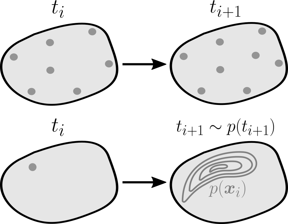
Figure 1: Top: Previous models assume dense observations at every time point and fixed spatiotemporal grids. Bottom: Our model works with extremely sparse observations and predicts where the next observations will happen.

In this work, we are dealing with the modeling of spatiotemporal dynamical systems whose dynamics are driven by partial differential equations. Such systems are ubiquitous and range from heat propagation in microstructures to the dynamics of oceanic currents. We use the data-driven modeling approach, where we observe a system at various time points and spatial locations and use the collected data to learn a model. In practice, the data is often collected by sensor networks that make measurements at random time points and random spatial locations. Such a measurement approach is used, for example, in crowdsourced earthquake monitoring where smartphones are used as measurement devices (Minson et al., 2015; Kong et al., 2016), in oceanographic monitoring where measurements are made by floating buoys (Albaladejo et al., 2010; Xu et al., 2014; Marin-Perianu et al., 2008), and for air pollution monitoring with vehicle-mounted sensors (Ma et al., 2008; Ghanem et al., 2004). This approach offers several advantages as it needs no sensor synchronization and allows the sensors to move freely. However, its random nature makes modeling more challenging as it requires us to capture both the system dynamics and the random observation process.

To the best of our knowledge, existing neural network-based methods cannot model randomly observed spatiotemporal dynamical systems, mainly for two reasons. First, they do not model observation times and locations, hence they cannot predict where and when the next observation will be made. Second, they assume the sensors form a fixed spatial grid and record data simultaneously, which is not the case in our setup where the data could come from as little as a single sensor at each time point (Fig. 1). For example, some earlier methods assume the observations are made on a fixed and regular spatiotemporal grid (Long et al., 2018; Geneva and Zabaras, 2020), other methods can handle irregular, but still fixed, observation locations (Iakovlev et al., 2020; Lienen and Günnemann, 2022), and other works go further and allow the observation locations to change over time (Pfaff et al., 2020; Yin et al., 2022) but fix the observation times and assume dense observations. Whereas, another line of research has proposed methods that model only the spatiotemporal observation process (Chen et al., 2020; Zhu et al., 2021; Zhou et al., 2022; Zhou and Yu, 2023; Du et al., 2016).

We fill the existing gap and propose a model for randomly observed spatiotemporal dynamical systems. Our model uses ideas from amortized variational inference (Kingma and Welling, 2013), neural differential equations (Chen et al., 2018; Rackauckas et al., 2020), neural point processes (Mei and Eisner, 2017; Chen et al., 2020), and implicit neural representations (Chen et al., 2022; Yin et al., 2022) to efficiently learn the underlying system dynamics as well as to model the random observation process. Our model maps initial observations to the latent initial state via a Transformer encoder (Vaswani et al., 2017). Then, it computes the latent trajectory using neural ODEs (Chen et al., 2018). Finally, it uses implicit neural representations and points along the latent trajectory to parameterize the point process and observation distribution. Our model shows strong empirical results outperforming other models from the literature on challenging spatiotemporal datasets.

2 Background

2.1 Spatiotemporal Point Processes

Spatiotemporal point processes (STPP) model sequences of events occurring in space and time. Each event has an associated event time $t_{i}\in\mathbb{R}_{\geq 0}$ and event location ${\bm{x}}_{i}\in\mathbb{R}^{d}$. Given an event history $\mathcal{H}_{t}\triangleq\{(t_{i},{\bm{x}}_{i})\ |\ t_{i}<t\}$ with all events up to time $t$, we can characterize an STPP by its conditional intensity function

$$\lambda^{*}(t,{\bm{x}})\triangleq\lim_{\delta t\downarrow 0,\ \delta r\downarrow 0}\frac{\mathbb{P}(t_{i}\in[t,t+\delta t],{\bm{x}}_{i}\in B_{\delta r}({\bm{x}})|\mathcal{H}_{t})}{\delta t|B_{\delta r}({\bm{x}})|},$$ (1)

where $\delta t$ denotes an infinitesimal time interval, and $B_{\delta r}({\bm{x}})$ denotes a $\delta r$-ball centered at ${\bm{x}}$. Given a history $\mathcal{H}_{t}$ with $i-1$ events, $\lambda^{*}(t,{\bm{x}})$ describes the instantaneous probability of the next, $i$th, event occurring at time $t$ and location ${\bm{x}}$. Given a sequence of $N$ events $\{(t_{i},{\bm{x}}_{i})\}_{i=1}^{N}$ on a bounded domain $A\subset[0,T]\times\mathbb{R}^{d}$, the log-likelihood for the STPP is evaluated as (Daley et al., 2003)

$$\log p(\{(t_{i},{\bm{x}}_{i})\}_{i=1}^{N})=\sum_{i=1}^{N}{\log\lambda^{*}(t_{i},{\bm{x}}_{i})}-\int_{A}{\lambda^{*}(t,{\bm{x}})d{\bm{x}}dt}.$$ (2)

2.2 Ordinary and Partial Differential Equations

Given a deterministic continuous-time dynamic system with state ${\bm{z}}(t)$, we can describe the evolution of its state in terms of an ordinary differential equation (ODE)

$$\frac{d{\bm{z}}(t)}{dt}=f(t,{\bm{z}}(t)).$$ (3)

For an initial state ${\bm{z}}_{1}$ at time $t_{1}$ we can solve the ODE to obtain the system state ${\bm{z}}(t)$ at later times $t>t_{1}$. The solution exists and is unique if $f$ is continuous in time and Lipschitz continuous in state (Coddington et al., 1956), and can be obtained either analytically or using numerical ODE solvers (Heirer et al., 1987). In this work we solve ODEs numerically using ODE solvers from torchdiffeq (Chen, 2018) package. Similarly, the dynamics of spatiotemporal systems with state ${\bm{z}}(t,{\bm{x}})$ defined over both space and time is described in terms of a partial differential equation (PDE)

$$\frac{\partial{\bm{z}}(t,{\bm{x}})}{\partial t}=F(t,{\bm{x}},{\bm{z}}(t,{\bm{x}}),\nabla{\bm{z}}(t,{\bm{x}}))$$ (4)

which incorporates both temporal and spatial derivatives, indicated by $\frac{\partial}{\partial t}$ and $\nabla$, respectively.

3 Problem Setup

In this work, we model spatiotemporal systems from data. The data consists of multiple trajectories collected by observing the system over a period of time. A trajectory consists of $N$ triplets $\{(t_{i},{\bm{x}}_{i},{\bm{y}}_{i})\}_{i=1}^{N}$, where ${\bm{y}}_{i}\in\mathbb{R}^{d_{\bm{y}}}$ is a system observation, with $t_{i}\in\mathbb{R}_{\geq 0}$ and ${\bm{x}}_{i}\in\mathbb{R}^{d_{\bm{x}}}$ being the corresponding observation time and location. The number of observations $N$ can change across different trajectories in the dataset. Due to randomness of the observation process we assume the observation times and locations do not overlap (neither within a trajectory nor across trajectories), resulting in a single observation ${\bm{y}}_{i}$ per time point and location. For brevity, we describe our method for a single observed trajectory, but extension to multiple trajectories is straightforward.

We assume the data generating process (DGP) involves a latent state ${\bm{u}}(t,{\bm{x}})\in\mathbb{R}^{d_{{\bm{u}}}}$ that is defined for $t\in\mathbb{R}_{\geq 0}$ and ${\bm{x}}\in\mathbb{R}^{d_{\bm{x}}}$. We assume the following DGP with some initial time $t_{1}$:

$${\bm{u}}(t_{1},\cdot) \sim p({\bm{u}}),\quad\frac{\partial{\bm{u}}(t,{\bm{x}})}{\partial t}=F({\bm{u}}(t,{\bm{x}}),\nabla{\bm{u}}(t,{\bm{x}}))),$$ (5)

$$t_{i},{\bm{x}}_{i} \sim\mathrm{nhpp}(\lambda({{\bm{u}}(t,{\bm{x}})})),\quad i=1,\dots,N,$$ (6)

$${\bm{y}}_{i} \sim p({\bm{y}}_{i}|g({\bm{u}}(t_{i},{\bm{x}}_{i}))),\quad i=1,\dots,N.$$ (7)

In that process, we first sample the latent field ${\bm{u}}(t_{1},\cdot)$ from $p({\bm{u}})$ and then specify its dynamics by a PDE (Eq. 5). Next, we sample the observation times $t_{i}$ and locations ${\bm{x}}_{i}$ from a non-homogeneous Poisson process (nhpp) with intensity $\lambda$ that is a function of the latent state (Eq. 6). Finally, we sample ${\bm{y}}_{i}$ from the observation distribution parameterized by a function $g$ (Eq. 7). All datasets in this work were generated according to this process (see Appendix A for details). We assume the data generating process is fully unknown, and our goal is to construct and learn its model from the data.

Limitations.

Using Poisson process for sampling event times and locations can be seen as a limitation in some applications because the assumption of non-overlapping time points may not hold in some real-world scenarios where effectively simultaneous observations might occur. Similarly, the lack of interaction between the event occurrence and system dynamics may not hold if observations affect the system, for example by triggering human actions or affecting sensor availability.

4 Methods

In this section we describe our proposed model, its components, and the parameter inference method.

4.1 Model

Our goal is to model data generated by the true space-time continuous DGP (Eqs. 5-7). Our generative model is defined as:

$${\bm{z}}(t_{1}) \sim p({\bm{z}}(t_{1})),\quad\frac{d{\bm{z}}(\tau)}{dt}=f({\bm{z}}(\tau)),$$ (8)

$${\bm{u}}(t,x) =\phi({\bm{z}}(t),{\bm{x}}),$$ (9)

$$t_{i},{\bm{x}}_{i} \sim\mathrm{nhpp}(\lambda({{\bm{u}}(t,{\bm{x}})})),\quad i=1,\dots,N,$$ (10)

$${\bm{y}}_{i} \sim p({\bm{y}}_{i}|g({\bm{u}}(t_{i},{\bm{x}}_{i}))),\quad i=1,\dots,N.$$ (11)

We describe each of the model components (Eqs. 8-11) in detail below. A diagram of our model is shown in Figure 2.

Latent dynamics (Eq. 8).

Our goal is to model the latent PDE dynamics of the DGP (Eq. 5). To that end, we introduce a low-dimensional temporal latent state ${\bm{z}}(\tau)\in\mathbb{R}^{d_{\bm{z}}}$ with $\tau\in\mathbb{R}_{\geq 0}$ that encodes the spatiotemporal field ${\bm{u}}(\tau,\cdot)$, and introduce a neural network parameterized ODE governing its dynamics (Eq. 8). We use a low-dimensional latent state because it allows to simulate the dynamics considerably quicker than a full-grid spatiotemporal discretization (Wu et al., 2022; Yin et al., 2022). We observed that the simulation times to numerically solve the ODE were long and increasing with the number of observations. We found that this happens because of a bottleneck in existing ODE solvers caused by extremely dense time grids (such as in Fig. 3). Such time grids force the ODE solver to choose small step sizes which prevents it from adaptively selecting the optimal step size thus reducing its efficiency. To improve the computational efficiency, we move away from the original dense time grid $t_{1},\dots,t_{N}$ to an auxiliary sparse grid $\tau_{1},\dots,\tau_{n}$, with $n\ll N$, where the first and last time points coincide with the original grid: $\tau_{1}=t_{1}$, $\tau_{n}=t_{N}$ (see Fig. 2). Then, we numerically solve for the latent state ${\bm{z}}(t)$ only at the sparse grid, which allows the ODE solver to choose the optimal step size and results in approximately an order of magnitude (up to 9x) faster simulations (see Sec. 5). Finally, we use the latent state evaluations ${\bm{z}}(\tau_{1}),\dots,{\bm{z}}(\tau_{n})$ to approximate the original latent state ${\bm{z}}(t)$ at any time point via interpolation as $\tilde{{\bm{z}}}(t)=\mathrm{interpolate}(t;{\bm{z}}(\tau_{1}),\dots,{\bm{z}}(\tau_{n}))$.

Latent state decoding (Eq. 9).

Next, we need to recover the latent spatiotemporal state ${\bm{u}}(t,{\bm{x}})$ from the low-dimensional representation $\tilde{{\bm{z}}}(t)$. We define the latent spatiotemporal state ${\bm{u}}(t,{\bm{x}})$ as a function $\phi(\tilde{{\bm{z}}}(t),{\bm{x}})$ of the latent state $\tilde{{\bm{z}}}(t)$ and evaluation location ${\bm{x}}$ (Eq. 9). In particular, we parameterize $\phi(\tilde{{\bm{z}}}(t),{\bm{x}})$ by an MLP which takes $\tilde{{\bm{z}}}(t)+\mathrm{proj}({\bm{x}})$ as the input and maps it directly to ${\bm{u}}(t,{\bm{x}})$, where $\mathrm{proj}({\bm{x}})\in\mathbb{R}^{d_{\bm{z}}}$ is a trainable linear mapping of ${\bm{x}}$ to $\mathbb{R}^{d_{\bm{z}}}$. This formulation results in space-time continuous ${\bm{u}}(t,{\bm{x}})$ which can be evaluated at any time point and spatial location, which is required to define the intensity function $\lambda({\bm{u}}(t,{\bm{x}}))$ and observation function $g({\bm{u}}(t,{\bm{x}}))$.

Intensity function (Eq. 10).

We parameterize the intensity function $\lambda({\bm{u}}(t,{\bm{x}}))$ by an MLP which takes ${\bm{u}}(t,{\bm{x}})$ as the input and maps it to intensity of the Poisson process (Eq. 10). To ensure non-negative values of the intensity function and improve its numerical stability we further exponentiate the output of the MLP and add a small constant to it.

Observation function (Eq. 11).

The observation function $g({\bm{u}}(t,{\bm{x}}))$ maps the latent spatiotemporal state ${\bm{u}}(t,{\bm{x}})$ to parameters of the observation model (Eq. 11). Therefore, its exact structure depends on the observation model. In this work the observation model is a normal distribution, where the variance is fixed and the observation function $g({\bm{u}}(t,{\bm{x}}))$ returns the mean.

Details of the model definition and parameterization can be found in Appendix B and C.

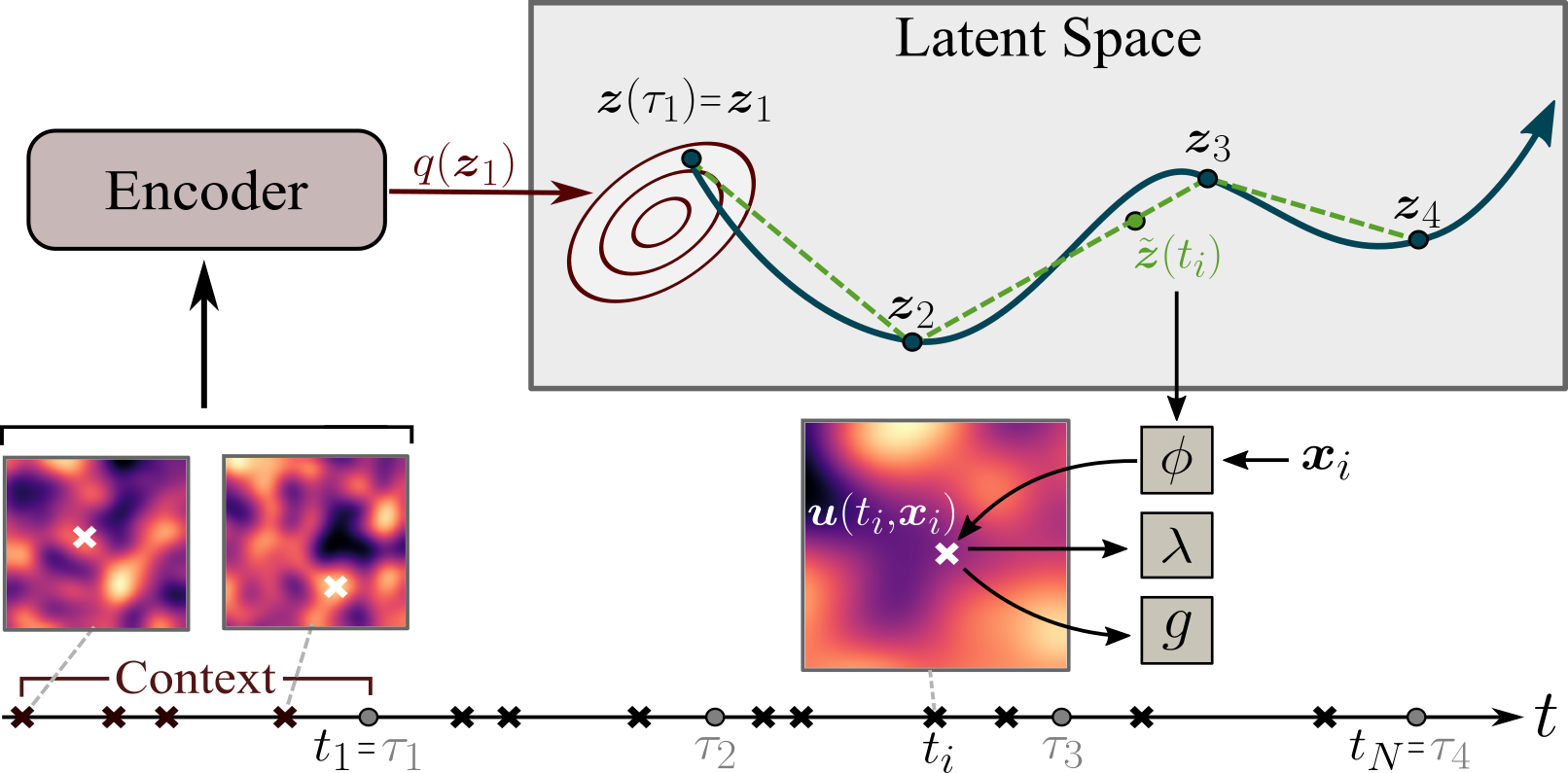
Figure 2: Diagram of our model. Black crosses indicate observation times, while white crosses indicate observation locations. The initial observations (context) are mapped by the encoder to the distribution of the latent initial state $q({\bm{z}}_{1})$. The initial state ${\bm{z}}_{1}$ is then sampled from that distribution and evolved through time using neural ODEs. For computational efficiency, the latent trajectory is evaluated only at the sparse time grid $\tau_{1},\dots,\tau_{n}$ and the latent state at other time points is evaluated via interpolation $\tilde{{\bm{z}}}(t)$. The latent state $\tilde{{\bm{z}}}(t)$ is then mapped by $\phi$ to the spatiotemporal state ${\bm{u}}(t,{\bm{x}})$, which is used to parameterize the point process and observation distribution (via mappings $\lambda$ and $g$, respectively) for predicting subsequent observation times and locations.

4.2 Parameter and Latent State Inference

We infer the model parameters and posterior of the latent initial state ${\bm{z}}_{1}\triangleq{\bm{z}}(t_{1})$ using amortized variational inference (Kingma and Welling, 2013). To approximate the posterior of ${\bm{z}}_{1}$ we define an approximate posterior distribution $q({\bm{z}}_{1};\psi)$ with local variational parameters $\psi$. Since there are multiple trajectories in the dataset and each trajectory has its own initial state, we need to define and optimize $\psi$ separately for each trajectory. To avoid optimizing $\psi$ for each trajectory we use amortization and define $\psi$ as the output of an encoder

$$\psi=\mathrm{Encoder}(\{t_{i},{\bm{x}}_{i},{\bm{y}}_{i}\}_{i=1}^{N_{\mathrm{ctx}}}),$$ (12)

which maps initial observations $\{t_{i},{\bm{x}}_{i},{\bm{y}}_{i}\}_{i=1}^{N_{\mathrm{ctx}}}$ (or the latest $N_{\mathrm{ctx}}$ observations, which we call the context) to the local variational parameters. The context size is defined by $N_{\mathrm{ctx}}$ and could be different for each trajectory (see Appendix A for details). We discuss the structure of the encoder in the next section.

In variational inference we minimize the Kullback-Leibler divergence between the approximate posterior $q({\bm{z}}_{1};\psi)$ and the true posterior $p({\bm{z}}_{1}|\{t_{i},{\bm{x}}_{i},{\bm{y}}_{i}\}_{i=1}^{N_{\mathrm{ctx}}})$ (Blei et al., 2017):

$$\mathrm{KL}\left[q({\bm{z}}_{1};\psi)\lVert p({\bm{z}}_{1}|\{t_{i},{\bm{x}}_{i},{\bm{y}}_{i}\}_{i=1}^{N_{\mathrm{ctx}}})\right],$$ (13)

which is equivalent to maximizing the evidence lower bound (ELBO), which for our model is

$$\mathcal{L} =\underbrace{\sum_{i=1}^{N}{\mathbb{E}_{q({\bm{z}}_{1};\psi)}\left[\ln p({\bm{y}}_{i}|t_{i},{\bm{x}}_{i},{\bm{z}}_{1})\right]}}_{\textit{(i)}\text{ Expected observation log-lik.}}+\underbrace{\mathbb{E}_{q({\bm{z}}_{1};\psi)}\left[\sum_{i=1}^{N}\ln\lambda({\bm{u}}(t_{i},{\bm{x}}_{i}))-\int{\lambda({\bm{u}}(t,{\bm{x}}))d{\bm{x}}dt}\right]}_{\textit{(ii)}\text{ Expected STPP log-lik.}}$$ (14)

$$\quad-\underbrace{\mathrm{KL}[q({\bm{z}}_{1};\psi)\lVert p({\bm{z}}_{1})].}_{\textit{(iii)}\text{ KL between prior and posterior}}$$ (15)

The ELBO is maximized wrt. the model and encoder parameters. Appendix B contains detailed derivation of the ELBO, and fully specifies the model and the approximate posterior. While the term (iii) can be computed analytically, computation of terms (i) and (ii) involves approximations: Monte Carlo integration for the expectations and intensity integral, and numerical ODE solvers for the solution of the initial value problems. Appendix B details the computation of ELBO.

4.3 Encoder

Our encoder maps the context $\{t_{i},{\bm{x}}_{i},{\bm{y}}_{i}\}_{i=1}^{N_{\mathrm{ctx}}}$ to the local variational parameters $\psi$ of $q({\bm{z}}_{1};\psi)$ using Eq. 12. The encoder works by first mapping elements of the context into a high-dimensional feature space, then processing the resulting sequence using a stacks of transformer encoder layers (Vaswani et al., 2017), and finally mapping the transformer’s output to variational parameters $\psi$. Next, we discuss this process in more details.

First, we convert the context sequence $\{t_{i},{\bm{x}}_{i},{\bm{y}}_{i}\}_{i=1}^{N_{\mathrm{ctx}}}$ to a sequence of vectors $\{{\bm{b}}_{i}\}_{i=1}^{N_{\mathrm{ctx}}}$, where

$${\bm{b}}_{i}=\mathrm{proj}(t_{i})+\mathrm{proj}({\bm{x}}_{i})+\mathrm{proj}({\bm{y}}_{i}),$$ (16)

with $\mathrm{proj}$ being separate trainable linear projections. We do not add positional encodings since $t_{i}$ and ${\bm{x}}_{i}$ already provide all required positional information. We further add an aggregation token [AGG] with a learnable representation and obtain the following input sequence: $\{\{{\bm{b}}_{i}\}_{i=1}^{N_{\mathrm{ctx}}},\text{[AGG]}\}$. Next, a stack of transformer encoder layers processes that input sequence into the output sequence $\{\{\overline{{\bm{b}}}_{i}\}_{i=1}^{N_{\mathrm{ctx}}},\overline{\text{[AGG]}}\}$. Finally, we map the output aggregation token $\overline{\text{[AGG]}}$ to the variational parameters $\psi$. This mapping depends on the form of the approximate posterior (see Appendix B for detailed specification of the mapping).

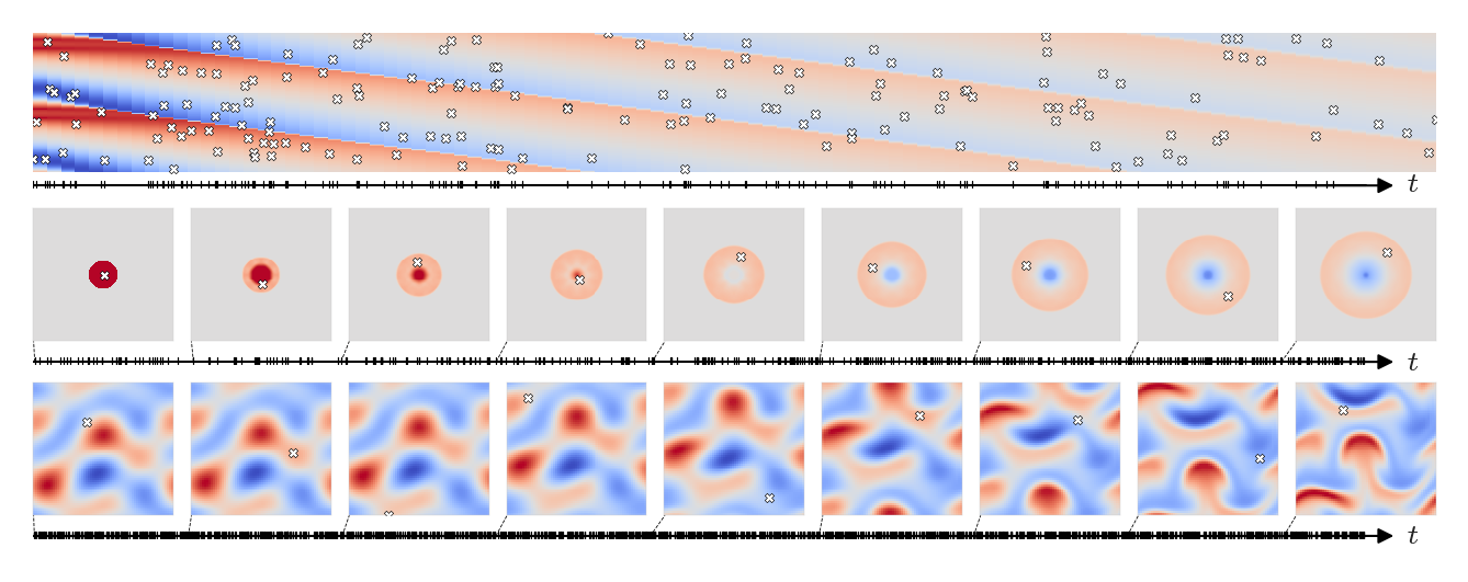
Figure 3: Examples of trajectories from our datasets. White crosses indicate the observation locations ${\bm{x}}$, marks on the horizontal time grid indicate the corresponding observation times $t$, and color-coded fields denote the system state with observations ${\bm{y}}$ at white crosses $(t,{\bm{x}})$. Top: Burger’s (1D) dataset. The whole trajectory is plotted, with 1-D measurement location ${\bm{x}}$ along the vertical and time $t$ along the horizontal directions. Middle and Bottom: Shallow Water (2D) and Navier-Stokes (2D) datasets, respectively. Due to the 2D nature of the systems, only snapshots of the system state are plotted.

5 Experiments

In this section we demonstrate properties of our method and compare it against other methods from the literature. Our datasets are generated by three commonly-used PDE systems: Burgers’ (models nonlinear 1D wave propagation), Shallow Water (models 2D wave propagation under the gravity), and Navier-Stokes with transport (models the spread of a pollutant in a liquid over a 2D domain). The observation times and locations are sampled from a non-homogeneous Poisson process with state-dependent intensity function using the thinning algorithm (Lewis and Shedler, 1979). See Appendix A for details about the dataset generation. Figure 3 shows examples of trajectories from the datasets. For all datasets our model has at most 3 million parameters, and training takes at most 1.5 hours on a single GeForce RTX 3080 GPU. The training is done for 25k iterations with learning rate 3e-4 and batch size 32. We use the adaptive ODE solver (dopri5) from torchdiffeq package with relative and absolute tolerance set to 1e-5. As performance metrics we use mean absolute error (MAE) for the observations ${\bm{y}}_{i}$, and event-averaged log-likelihood of the point process for $t_{i}$ and ${\bm{x}}_{i}$, both evaluated on the test set. See Appendix C for our training setup and for details about the model architecture and hyperparameters.

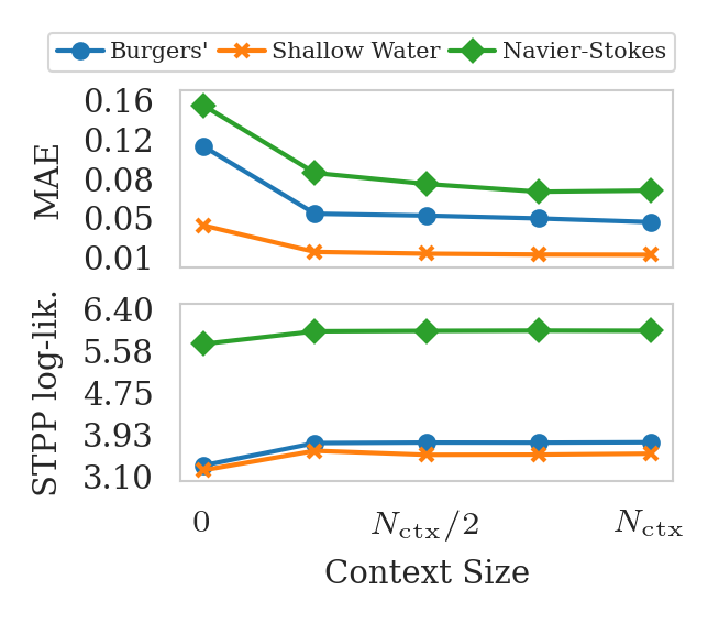
Figure 4: Test MAE and log-likelihood vs context size.

Context Size.

Our encoder maps the initial observations (context) $\{t_{i},{\bm{x}}_{i},{\bm{y}}_{i}\}_{i=1}^{N_{\mathrm{ctx}}}$ to parameters $\psi$ of the approximate posterior $q({\bm{z}}_{1};\psi)$. Here we look at how accuracy of the state predictions and process likelihood is affected by the context size. We train and test our model with different context sizes: full ($N_{\mathrm{ctx}}$ to 1), half of the context ($N_{\mathrm{ctx}}/2$ to 1), etc., and show the results in Figure 4. We see that both MAE and process likelihood quickly improve as we increase the context size, but the improvements saturate for larger contexts. This indicates that the encoder mostly uses observations that are close to the time point at which the latent state should be inferred, and does not utilize observations that are too far away from it.

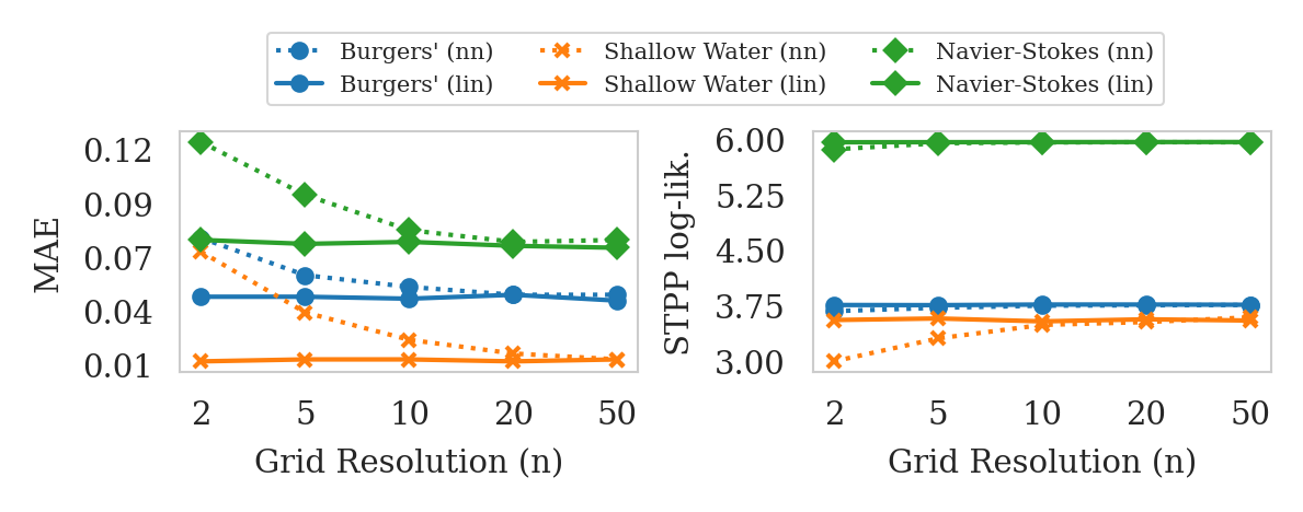
[0.62] [0.3] Dataset Interp. Seq. Burgers’ 0.007 0.018 Shallow Water 0.011 0.045 Navier-Stokes 0.012 0.108

Figure 5: Test MAE and process log-likelihood for different temporal grid resolutions ($n$) and interpolation methods (nn = nearest neighbor, lin = linear).

Figure 6: Latent state evaluation time (sec), interpolation vs sequential method. Averaged time over all trajectories.

Latent State Interpolation.

As discussed in Section 4.1, we do not evaluate the latent state at the full time grid $t_{1},\dots,t_{N}$ using the ODE solver (we call it the sequential method). Instead, we use the ODE solver to evaluate the latent state only at a sparser time grid $\tau_{1},\dots,\tau_{n}$, and then interpolate the evaluations to the full grid. Here we look at how this approach affects training times, and investigate the effects of the grid resolution $n$ and different interpolation methods. We vary the resolution from coarse $n=2$ to fine $n=50$, and test nearest neighbor and linear interpolation methods. Figure 6 shows that both MAE and process log-likelihood improve with the grid resolution, but only when we use nearest neighbor interpolation. With linear interpolation, the model achieves its best performance with just $n=2$, meaning that interpolation is done between only two points in the latent space, and further increasing the resolution does not improve the results. Both interpolation methods achieve the same optimal performance when $n\geq 20$. Furthermore, Table 6 shows that our method results in up to 9x faster latent state evaluation than the sequential method, which in our case translates in up to 4x faster training (computed with $n=20$).

Interaction Between Observation and Process Models.

Table 1: Test MAE and log-likelihood of the full model, and after removing the point process (-STPP) or the observation model (-Obs.).

Dataset	MAE	MAE (-STPP)	Log-lik.	Log-lik (-Obs.)
Burgers’	0.042	0.043	3.77	3.70
Shallow Water	0.012	0.012	3.67	3.56
Navier-Stokes	0.071	0.071	5.96	5.92

In our model the observation times and locations are modeled by a point process model (Eq. 10), while observations are modeled by an observation model (Eq. 11). Intuitively, one could expect some interaction between them and ask the question of how important is one model for the performance of the other. In this experiment we look at the effect of removing the point process model on the performance of the observation model and vice versa. We remove the point process model by removing Eq. 10 from our model, so that we do not model the observation times and locations. Similarly, we remove the observation model by removing Eq. 11 from our model and also removing observations ${\bm{y}}_{i}$ from our data, so that there is no information about the observation values. In Table 1 we show that removing the point process model seems to have practically no effect on MAE, while removing the observation model decreases the process likelihood. This shows that if we know the system states we can model the observation times and locations more accurately.

Comparison to Other Methods.

We compare our method against two groups of methods from the literature. The first group consists of neural spatiotemporal dynamic models that can model only the observations ${\bm{y}}_{i}$ but not the time points and spatial locations. This group includes FEN (Lienen and Günnemann, 2022) (graph neural network-based model, simulates the system dynamics at every point on the spatial grid), NSPDE (Salvi et al., 2022) (space- and time-continuous model simulating the dynamics in the spectral domain), and CNN-ODE (our simple baseline that uses a CNN encoder/decoder to map observations to/from the latent space, and uses neural ODEs (Chen et al., 2018) to model the latent space dynamics). Note that due to their assumption about multiple observations per time point, dynamic models require time binning (see Appendix C.4). The second group consists of neural spatiotemporal point processes that model only the observation times and locations. This group consists of DSTPP (Yuan et al., 2023), NSTPP (Chen et al., 2020), and AutoSTPP (Zhou and Yu, 2023). We also provide simple baselines for both groups: median predictor for dynamic models, and constant (learnable) intensity for the point process group. Hyperparameters of each method were tuned for the best performance. See Appendix C.4 for details about the models and hyperparameters used.

Table 2 shows the comparison results. We see that most methods from the first group perform rather poorly and fail to beat even the MAE of the median predictor, with the simple CNN-ODE model showing the best results. However, CNN-ODE still performs considerably worse than our model likely because of the loss of information caused by time binning. In the second group most methods showed poor results and failed to beat the simple constant intensity baseline, however AutoSTPP showed very strong performance, although still not outperforming our method.

These experiments show the challenging nature of modeling randomly observed dynamical systems, and demonstrate our method’s properties and strong performance.

Table 2: Model comparisons. MAE and Log-lik (per event) on test data. The first group of methods (FEN, NSPDE, CNN-ODE) contains neural spatiotemporal dynamical models. The second group (DSTPP, NSTPP, AutoSTPP) contains neural spatiotemporal point process models. Error bars represent one standard error calculated over 5 realizations of a random seed controlling the model initialization.

Model	Burgers’		Shallow Water		Navier-Stokes
	MAE ($\downarrow$)	Log-lik. ($\uparrow$)	MAE ($\downarrow$)	Log-lik. ($\uparrow$)	MAE ($\downarrow$)	Log-lik. ($\uparrow$)
Median Pred.	0.161	-	0.148	-	0.155	-
FEN	N/A	-	$0.336\pm 0.008$	-	$0.158\pm 0.006$	-
NSPDE	$0.166\pm 0.002$	-	$0.339\pm 0.002$	-	$0.098\pm 0.001$	-
CNN-ODE	$0.076\pm 0.000$	-	$0.032\pm 0.001$	-	$0.077\pm 0.002$	-
Const. Intensity	-	3.59	-	2.02	-	5.86
DSTPP	-	$0.67\pm 0.13$	-	$0.08\pm 0.04$	-	$0.41\pm 0.04$
NSTPP	-	$2.35\pm 0.06$	-	$1.53\pm 0.13$	-	$3.83\pm 0.14$
AutoSTPP	-	N/A	-	$3.37\pm 0.01$	-	$5.91\pm 0.01$
Ours	$\bm{0.043}\pm\bm{0.002}$	$\bm{3.77}\pm\bm{0.02}$	$\bm{0.012}\pm\bm{0.001}$	$\bm{3.62}\pm\bm{0.05}$	$\bm{0.071}\pm\bm{0.001}$	$\bm{5.96}\pm\bm{0.01}$

6 Related Work

Neural Point Processes.

Traditionally, intensity functions are simple parametric functions incorporating domain knowledge about the system being modeled. While simple and interpretable, this approach might require strong domain knowledge and might have limited expressivity due to overly simplistic form of the intensity function. These limitations lead to the development of neural point processes which parameterize the intensity function by a neural network, leading to improved flexibility and expressivity. For example Mei and Eisner (2017); Omi et al. (2019); Jia and Benson (2019); Zuo et al. (2020) use neural networks to model time-dependent intensity functions in a flexible and efficient manner, with neural architectures ranging from recurrent neural networks to transformers and neural ODEs. These techniques consistently outperform classical intensity parameterizations and do not require strong domain expertise to choose the right form of the intensity function. Other works extend this idea to marked point processes where intensity is a function of time and also of a discrete or continuous mark. For example, Chen et al. (2020); Zhu et al. (2021); Zhou et al. (2022); Zhou and Yu (2023); Yuan et al. (2023) use spatial coordinates as a mark and model the intensity using a wide range of methods aimed at improving flexibility and efficiency. Works such as Du et al. (2016); Xiao et al. (2019); Boyd et al. (2020) use discrete observations as marks, and Sharma et al. (2018) use continuous marks with underlying dynamic model, which makes their work most similar to ours, with major differences related to the model, training process, and them working only with temporal processes, whereas we are dealing with more general spatiotemporal processes.

Neural Spatiotemporal Dynamic Models.

To model the spatiotemporal dynamics our method uses the “encode-process-decode” approach employed in many other works. The main idea of the approach consists of taking a set of initial observations and using it to estimate the latent initial state. A dynamics function is then used to map the latent state forward in time to other time points either discretely (Long et al., 2018; Han et al., 2022; Wu et al., 2022) or continuously (Yildiz et al., 2019; Salvi et al., 2022). Finally, the latent state is mapped to the observations using discrete (Yildiz et al., 2019; Wu et al., 2022) or continuous (Yin et al., 2022; Chen et al., 2022) decoder. Such methods assume multiple observations per time point and do not model the observation times and locations.

Implicit Neural Representations.

Our model represents the continuous latent spatiotemporal state ${\bm{u}}(t,{\bm{x}})$ in terms of a function $\phi(\tilde{{\bm{z}}}(t),{\bm{x}})$. This approach to representing continuous field is called implicit neural representations (Park et al., 2019; Chen and Zhang, 2019; Mescheder et al., 2019; Chibane et al., 2020), and it has found applications in many other works related to modeling of spatiotemporal systems (Chen et al., 2022; Yin et al., 2022).

7 Conclusion

In this work, we developed a method for modeling of randomly observed spatiotemporal dynamical systems. Along with our method, we proposed an interpolation-based technique to greatly speed up its training times. In the experiments we showed that our method effectively utilizes the context size of various length to improve accuracy of the initial state inference, and that it uses the system state observations to improve the modeling of observation times and locations. We further demonstrated that our method achieves strong performance on challenging spatiotemporal datasets and outperforms other methods from the literature.

Appendix A Data

As described in Section 3, we assume the following data generating process

$${\bm{u}}(t_{1},\cdot)\sim p({\bm{u}}),\quad\frac{\partial{\bm{u}}(t,{\bm{x}})}{\partial t}=F({\bm{u}}(t,{\bm{x}}),\nabla{\bm{u}}(t,{\bm{x}}))),$$ (17)

$$t_{i},{\bm{x}}_{i}\sim\mathrm{nhpp}(\lambda({{\bm{u}}(t,{\bm{x}})})),\quad i=1,\dots,N,$$ (18)

$${\bm{y}}_{i}\sim p({\bm{y}}_{i}|g({\bm{u}}(t_{i},{\bm{x}}_{i}))),\quad i=1,\dots,N,$$ (19)

We selected three commonly used PDE systems: Burgers’, Shallow Water, and Navier-Stokes with transport. Next we discuss the data generating process for each dataset.

A.1 Burgers’

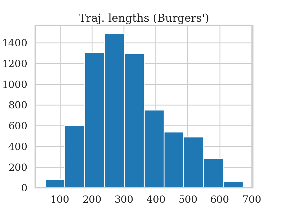
Figure 7: Trajectory lengths for Burgers’ dataset.

The Burgers’ system in 1D is characterized by a 1-dimensional state $u(t,x)$ and the following PDE dynamics:

$$\frac{\partial u}{\partial t}+u\frac{\partial u}{\partial x}=\nu\frac{\partial^{2}u}{\partial t^{2}},$$ (20)

where $\nu$ is the diffusion coefficient. We obtain data for this system from the PDEBench dataset (Takamoto et al., 2022). The system is simulated on a time interval $[0,2]$ and on a spatial domain $[0,1]$ with periodic boundary conditions. The dataset contains 10000 trajectories, each trajectory is evaluated on a uniform temporal grid with 101 time points, and uniform spatial grid with 256 nodes.

Since the data is discrete, we define continuous field $u(t,x)$ by linearly interpolating the data across space and time. Next, we use the interpolant to define the intensity function

$$\lambda(u(t,x))=1600|u(t,x)|,$$ (21)

and use it to simulate the non-homogeneous Poisson process using the thinning algorithm (Lewis and Shedler, 1979). As the result, for each the 10000 trajectories, we obtain a sequence of time points and spatial locations $\{t_{i},x_{i}\}_{i=1}^{N}$, where $N$ can be different for each trajectory. Finally, we compute the observations as

$${\bm{y}}_{i}=u(t_{i},x_{i}).$$ (22)

We use the first 0.5 seconds as the context for the initial state inference, and further filter the dataset to ensure that each trajectory has at least 10 points in the context, resulting in approximately 7000 trajectories. We use 80%/10%/10% split for training/validation/testing.

A.2 Shallow Water

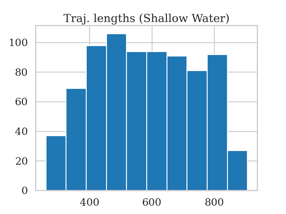
Figure 8: Trajectory lengths for Shallow Water dataset.

The Shallow Water system in 2D is characterized by a 3-dimensional state

$${\bm{u}}(t,x)=[h(t,{\bm{x}}),u(t,{\bm{x}}),v(t,{\bm{x}})]$$ (23)

and the following PDE dynamics:

$$\frac{\partial h}{\partial t}+\frac{\partial(hu)}{\partial x}+\frac{\partial(hv)}{\partial y}=0,$$ (24)

$$\frac{\partial u}{\partial t}+u\frac{\partial u}{\partial x}+v\frac{\partial u}{\partial y}+g\frac{\partial h}{\partial x}=0,$$ (25)

$$\frac{\partial v}{\partial t}+u\frac{\partial v}{\partial x}+v\frac{\partial v}{\partial y}+g\frac{\partial h}{\partial y}=0,$$ (26)

where $g$ is the gravitational acceleration, $h(t,{\bm{x}})$ is wave height, and $u(t,{\bm{x}})$ and $v(t,{\bm{x}})$ are horizontal and vertical velocities, respectively. We obtain data for this system from the PDEBench dataset (Takamoto et al., 2022). The system is simulated on a time interval $[0,1]$ and on a spatial domain $[-2.5,2.5]^{2}$. The dataset contains 1000 trajectories, each trajectory is evaluated on a uniform temporal grid with 101 time points, and uniform 128-by-128 spatial grid.

Since the data is discrete, we define continuous field ${\bm{u}}(t,x)$ by linearly interpolating the data across space and time. Next, we use the interpolant to define the intensity function

$$\lambda({\bm{u}}(t,{\bm{x}}))=500|h(t,{\bm{x}})-1|,$$ (27)

indicating that measurements are made only when the wave height is below or above the baseline of 1. We use the intensity function to simulate the non-homogeneous Poisson process using the thinning algorithm (Lewis and Shedler, 1979). As the result, for each of the 1000 trajectories, we obtain a sequence of time points and spatial locations $\{t_{i},x_{i}\}_{i=1}^{N}$, where $N$ can be different for each trajectory. Finally, we compute the observations as

$${\bm{y}}_{i}=h(t_{i},{\bm{x}}_{i}),$$ (28)

observing only the wave height.

We use the first 0.1 seconds as the context for the initial state inference, and further filter the dataset to ensure that each trajectory has at least 10 points in the context, resulting in approximately 800 trajectories. We use 80%/10%/10% split for training/validation/testing.

A.3 Navier-Stokes

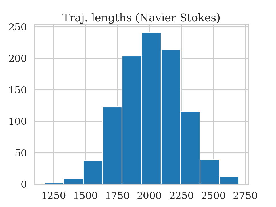
Figure 9: Trajectory lengths for Navier-Stokes dataset.

The Navier-Stokes system with a transport equation is characterized by a 4-dimensional state

$${\bm{u}}(t,{\bm{x}})=[c(t,{\bm{x}}),u(t,{\bm{x}}),v(t,{\bm{x}}),p(t,{\bm{x}})]$$ (29)

and the following PDE dynamics:

$$\frac{\partial u}{\partial x}+\frac{\partial v}{\partial y}=0,$$ (30)

$$\frac{\partial u}{\partial t}+u\frac{\partial u}{\partial x}+v\frac{\partial u}{\partial y}=-\frac{\partial p}{\partial x}+\nu\left(\frac{\partial^{2}u}{\partial x^{2}}+\frac{\partial^{2}u}{\partial y^{2}}\right),$$ (31)

$$\frac{\partial v}{\partial t}+u\frac{\partial v}{\partial x}+v\frac{\partial v}{\partial y}=-\frac{\partial p}{\partial y}+\nu\left(\frac{\partial^{2}v}{\partial x^{2}}+\frac{\partial^{2}v}{\partial y^{2}}\right)+c,$$ (32)

$$\frac{\partial c}{\partial t}=-u\frac{\partial c}{\partial x}-v\frac{\partial c}{\partial y}+\nu\left(\frac{\partial^{2}c}{\partial x^{2}}+\frac{\partial^{2}c}{\partial y^{2}}\right),$$ (33)

where the diffusion constant $\nu=0.002$, and $c(t,{\bm{x}})$ is concentration of the transported species, $p(t,{\bm{x}})$ is pressure, and $u(t,{\bm{x}})$ and $v(t,{\bm{x}})$ are horizontal and vertical velocities, respectively. For each trajectory, we start with zero initial velocities and pressure, and the initial scalar field $c_{0}(x,y)$ is generated as:

$$\tilde{c}_{0}(x,y)=\sum_{k,l=-N}^{N}{\lambda_{kl}\cos(2\pi(kx+ly))+\gamma_{kl}\sin(2\pi(kx+ly))},$$ (34)

$$c_{0}(x,y)=\frac{\tilde{c}_{0}(x,y)-\mathrm{min}(\tilde{c}_{0})}{\mathrm{max}(\tilde{c}_{0})-\mathrm{min}(\tilde{c}_{0})},$$ (35)

where $N=2$ and $\lambda_{kl},\gamma_{kl}\sim\mathcal{N}(0,1)$.

We use PhiFlow (Holl et al., 2020) to solve the PDEs. The system is simulated on a time interval $[0,1]$ and on a spatial domain $[0,1]^{2}$ with periodic boundary conditions. The solution is evaluated at randomly selected spatial locations and time points. We use $1089$ spatial locations and $25$ time points. The spatial and temporal grids are the same for all trajectories. The dataset contains 1000 trajectories.

Since the data is discrete, we define continuous field ${\bm{u}}(t,x)$ by linearly interpolating the data across space and time. Next, we use the interpolant to define the intensity function

$$\lambda({\bm{u}}(t,{\bm{x}}))=2000|c(t,{\bm{x}})|,$$ (36)

indicating that measurement intensity is proportional to the species concentration. We use the intensity function to simulate the non-homogeneous Poisson process using the thinning algorithm (Lewis and Shedler, 1979). As the result, for each of the trajectories, we obtain a sequence of time points and spatial locations $\{t_{i},x_{i}\}_{i=1}^{N}$, where $N$ can be different for each trajectory. Finally, we compute the observations as

$${\bm{y}}_{i}=c(t_{i},{\bm{x}}_{i}),$$ (37)

observing only the species concentrations.

We use the first 0.5 seconds as the context for the initial state inference, and further filter the dataset to ensure that each trajectory has at least 10 points in the context, resulting in all 1000 trajectories satisfying this condition. We use 80%/10%/10% split for training/validation/testing.

Appendix B Model, Posterior, and ELBO

B.1 Model

As described in Section 4.1 our model is defined as

$${\bm{z}}_{1}\sim p({\bm{z}}_{1}),\quad\frac{d{\bm{z}}(\tau)}{dt}=f({\bm{z}}(\tau)),$$ (38)

$$\tilde{{\bm{z}}}(t)=\mathrm{interpolate}(t;{\bm{z}}(\tau_{1}),\dots,{\bm{z}}(\tau_{n})),$$ (39)

$${\bm{u}}(t,x)=\phi(\tilde{{\bm{z}}}(t),{\bm{x}}),$$ (40)

$$t_{i},{\bm{x}}_{i}\sim\mathrm{nhpp}(\lambda({{\bm{u}}(t,{\bm{x}})})),\quad i=1,\dots,N,$$ (41)

$${\bm{y}}_{i}\sim p({\bm{y}}_{i}|g({\bm{u}}(t_{i},{\bm{x}}_{i}))),\quad i=1,\dots,N..$$ (42)

The corresponding joint distribution is

$$p({\bm{z}}_{1},\{t_{i},{\bm{x}}_{i},{\bm{y}}_{i}\}_{i=1}^{N})=p({\bm{z}}_{1})p(\{t_{i},{\bm{x}}_{i}\}_{i=1}^{N}|{\bm{z}}_{1})\prod_{i=1}^{N}{p({\bm{y}}_{i}|{\bm{z}}_{1},t_{i},{\bm{x}}_{i})},$$ (43)

where

$$p({\bm{z}}_{1})=\mathcal{N}(\bm{0},I),$$ (44)

$$p(\{t_{i},{\bm{x}}_{i}\}_{i=1}^{N}|{\bm{z}}_{1})=\prod_{i=1}^{N}{\lambda({\bm{u}}(t_{i},{\bm{x}}_{i}))}\exp{\left(-\int{\lambda({\bm{u}}(t,{\bm{x}}))d{\bm{x}}dt}\right)},$$ (45)

$$p({\bm{y}}_{i}|{\bm{z}}_{1},t_{i},{\bm{x}}_{i})=\mathcal{N}(g({\bm{u}}(t_{i},{\bm{x}}_{i})),\sigma_{{\bm{y}}}^{2}I),$$ (46)

where $\mathcal{N}$ is the normal distribution, $\bm{0}$ is a zero vector, and $I$ is the identity matrix. We set $\sigma_{{\bm{y}}}$ to $10^{-3}$.

B.2 Posterior

We define the approximate posterior with $\psi=[\psi_{\mu},\psi_{\sigma^{2}}]$ as

$$q({\bm{z}}_{1};\psi)=\mathcal{N}({\bm{z}}_{1}|\psi_{\mu},\mathrm{diag}(\psi_{\sigma^{2}})),$$ (47)

where $\mathcal{N}$ is the normal distribution, and $\mathrm{diag}(\psi_{\sigma^{2}})$ is a matrix with vector $\psi_{\sigma^{2}}$ on the diagonal.

As discussed in Section 4.3, the encoder maps the context $\{t_{i},{\bm{x}}_{i},{\bm{y}}_{i}\}_{i=1}^{N_{\mathrm{ctx}}}$ to the local variational parameters $\psi$ (which we break up into $[\psi_{\mu},\psi_{\sigma^{2}}]$). The encoder first converts the context sequence $\{t_{i},{\bm{x}}_{i},{\bm{y}}_{i}\}_{i=1}^{N_{\mathrm{ctx}}}$ to a sequence of vectors $\{{\bm{b}}_{i}\}_{i=1}^{N_{\mathrm{ctx}}}$ and then adds an aggregation token, which gives the following input sequence: $\{\{{\bm{b}}_{i}\}_{i=1}^{N_{\mathrm{ctx}}},\text{[AGG]}\}$. We pass it though the transformer encoder and read the value of the aggregation token at the last layer, which we denote by $\overline{\text{[AGG]}}$. Then, we map $\overline{\text{[AGG]}}$ to $[\psi_{\mu},\psi_{\sigma^{2}}]$ as follows:

$$\psi_{\mu}=\mathrm{Linear}(\overline{\text{[AGG]}}),$$ (48)

$$\psi_{\sigma^{2}}=\exp\left({\mathrm{Linear}(\overline{\text{[AGG]}})}\right),$$ (49)

where $\mathrm{Linear}$ are separate linear mappings.

B.3 ELBO

Given definitions in the previous sections, we can write the ELBO as

$$\mathcal{L} =\int q({\bm{z}}_{1})\ln{\frac{p({\bm{z}}_{1},\{t_{i},{\bm{x}}_{i},{\bm{y}}_{i}\}_{i=1}^{N})}{q({\bm{z}}_{1})}}d{\bm{z}}_{1}$$ (50)

$$=\int q({\bm{z}}_{1})\ln{\frac{\prod_{i=1}^{N}{p({\bm{y}}_{i}|{\bm{z}}_{1},t_{i},{\bm{x}}_{i})}p(\{t_{i},{\bm{x}}_{i}\}_{i=1}^{N}|{\bm{z}}_{1})p({\bm{z}}_{1})}{q({\bm{z}}_{1})}}d{\bm{z}}_{1}$$ (51)

$$=\int q({\bm{z}}_{1})\ln{\prod_{i=1}^{N}{p({\bm{y}}_{i}|{\bm{z}}_{1},t_{i},{\bm{x}}_{i})}}d{\bm{z}}_{1}$$ (52)

$$\quad+\int q({\bm{z}}_{1})\ln{p(\{t_{i},{\bm{x}}_{i}\}_{i=1}^{N}|{\bm{z}}_{1})}d{\bm{z}}_{1}$$ (53)

$$\quad+\int q({\bm{z}}_{1})\ln{\frac{p({\bm{z}}_{1})}{q({\bm{z}}_{1})}}d{\bm{z}}_{1}$$ (54)

$$=\underbrace{\sum_{i=1}^{N}{\mathbb{E}_{q({\bm{z}}_{1})}\left[\ln p({\bm{y}}_{i}|{\bm{z}}_{1},t_{i},{\bm{x}}_{i})\right]}}_{\mathcal{L}_{1}}$$ (55)

$$\quad+\underbrace{\mathbb{E}_{q({\bm{z}}_{1})}\left[\sum_{i=1}^{N}\ln\lambda({\bm{u}}(t_{i},{\bm{x}}_{i}))-\int{\lambda({\bm{u}}(t,{\bm{x}}))d{\bm{x}}dt}\right]}_{\mathcal{L}_{2}}$$ (56)

$$\quad-\underbrace{\mathrm{KL}[q({\bm{z}}_{1})\lVert p({\bm{z}}_{1})]}_{\mathcal{L}_{3}}.$$ (57)

$$=\mathcal{L}_{1}+\mathcal{L}_{2}-\mathcal{L}_{3}.$$ (58)

Computing ELBO.

We compute the ELBO as follows:

1. Compute local variational parameter from the context as
   $\psi_{\mu},\psi_{\sigma^{2}}=\mathrm{Encoder}(\{t_{i},{\bm{x}}_{i},{\bm{y}}_{i}\}_{i=1}^{N_{\mathrm{ctx}}})$

2. Sample the latent initial state as ${\bm{z}}_{1}\sim\mathcal{N}({\bm{z}}_{1}|\psi_{\mu},\mathrm{diag}(\psi_{\sigma^{2}}))$ using reparameterization

3. Evaluate ${\bm{z}}(\tau_{1}),\dots,{\bm{z}}(\tau_{n})$ by solving $\frac{d{\bm{z}}(\tau)}{dt}=f({\bm{z}}(\tau))$ with ${\bm{z}}_{1}$ as the initial condition. We solve the ODE using torchdiffeq package (Chen et al., 2018).

4. Compute the latent states $\tilde{{\bm{z}}}(t_{1}),\dots,\tilde{{\bm{z}}}(t_{N})$ via interpolation as
   $\tilde{{\bm{z}}}(t)=\mathrm{interpolate}(t;{\bm{z}}(\tau_{1}),\dots,{\bm{z}}(\tau_{n}))$

5. Compute ${\bm{u}}(t_{1},{\bm{x}}_{1}),\dots,{\bm{u}}(t_{N},{\bm{x}}_{N})$ as ${\bm{u}}(t_{i},{\bm{x}}_{i})=\phi(\tilde{{\bm{z}}}(t_{i}),{\bm{x}}_{i})$

6. Compute $\mathcal{L}_{1}$ using Monte Carlo integration

7. Compute $\mathcal{L}_{2}$ using Monte Carlo integration, with the intensity integral computed using torchquad (Gómez et al., 2024) package.

8. Compute $\mathcal{L}_{3}$ analytically

Sampling is done using reparametrization (Kingma and Welling, 2013) to allow for exact gradient evaluation via backpropagation. Monte Carlo integration is done using sample size of one.

Appendix C Experiments Setup

C.1 Datasets

See Appendix A for all details about dataset generation. For all datasets we use 80%/10%10% train/validation/test splits. The context size $N_{\mathrm{ctx}}$ is determined for each trajectory separately based on the time interval that we consider to be the context, for Burgers’ and Navier-Stokes it is the first 0.5 seconds (out of 2 seconds), while for Shallow Water it is 0.1 seconds (out of 1 second). Since the number of events occurring within this fixed time interval is different for each trajectory, the context size consequently differs across trajectories. See encoder architecture description below for details on how different context lengths are processed.

C.2 Training, Validation, and Testing

We use AdamW (Loshchilov and Hutter, 2017) optimizer with constant learning rate 3e-4 (we use linear warmup for first 250 iterations). We train for 25000 iterations, sampling a random minibatch from the training dataset at every iteration. We do not use any kind of scaling for the ELBO terms.

We compute validation error (MAE on observations) on a single random minibatch from the validation set every 125 iterations. We save the current model weights if the validation error averaged over last 10 validation runs is the smallest so far.

To simulate the model’s dynamics we use differentiable ODE solvers from torchdiffeq package (Chen et al., 2018). In particular, we use the dopri5 solver with $\text{rtol}=\text{atol}=10^{-5}$ without the adjoint method. To evaluate the intensity integral $\int{\lambda({\bm{u}}(t,{\bm{x}})d{\bm{x}}dt}$ we use Monte Carlo integration from the torchquad (Gómez et al., 2024) package with 32 randomly sampled points for training, and 256 randomly sampled points for testing, we found these sample sizes to be sufficient for producing small variance of the integral estimation in our case.

C.3 Encoder and Model Architectures

Encoder.

We use padding to efficiently handle input contexts of varying length. The time points, coordinates, and observations are linearly projected to the embedding space (128-dim for Burgers’ and Shallow Water, and 192-dim for Navier-Stokes). Then, the projections are summed and passed through a stack of transformer encoder layers (4 layers for Burgers’ and Shallow Water, and 5 layers for Navier-Stokes, 4 attention heads were used in all cases). We introduce a learnable aggregation token which we append at the end of each input sequence. The final layer’s output is read from the last token of the output sequence (corresponds to the aggregation token) and is mapped to the local variational parameters as discussed in Appendix B.

Model.

The dynamics function $f({\bm{z}}(t))$ is an MLP with 3 layers 368 neurons each, and GeLU (Hendrycks and Gimpel, 2016) nonlinearities. We set resolution of the uniform temporal grid $\tau_{1},\dots,\tau_{n}$ to $n=50$. The dynamics function maps the current latent state ${\bm{z}}(t)$ to its time derivative $\frac{d{\bm{z}}(t)}{dt}$, both are $d_{\bm{z}}$-dimensional vectors.

The function $\phi(\tilde{{\bm{z}}}(t),{\bm{x}})$ is an MLP with 3 hidden layers with width 368 for Burgers’, 256 for Shallow Water, and 512 for Navier-Stokes. We use GeLU (Hendrycks and Gimpel, 2016) nonlinearities. As the input the MLP takes the sum of $\tilde{{\bm{z}}}(t)\in\mathbb{R}^{d_{{\bm{z}}}}$ with $\mathrm{proj}({\bm{x}})\in\mathbb{R}^{d_{{\bm{z}}}}$, where $\mathrm{proj}$ is a linear projection, and maps the sum to the output ${\bm{u}}(t,{\bm{x}})\in\mathbb{R}^{d_{{\bm{u}}}}$.

The intensity function $\lambda({\bm{u}}(t,{\bm{x}}))$ is an MLP with 3 layers, 256 neurons each, and GeLU (Hendrycks and Gimpel, 2016) nonlinearities. We further exponentiate the output of the MLP and add a small constant (1e-4) to it to ensure the intensity is positive and to avoid numerical instabilities.

We set the observation function $g({\bm{u}}(t,{\bm{x}}))$ to the identity function, thus $g({\bm{u}}(t,{\bm{x}}))={\bm{u}}(t,{\bm{x}})$.

C.4 Model Comparison

C.4.1 Dynamic Spatiotemporal Models

In this section we discuss neural spatiotemporal models we used for the comparisons. But first, we discuss data preprocessing that we do in order to make these models applicable.

Data Preprocessing.

All models in this section assume that dense observations are available at every time point, and some further assume the observations are located on a uniform spatial grid. To make our data satisfy these requirements we use time binning and spatial interpolation. First, we use time binning and divide the original time grid into 10 bins and group all time points into 10 groups based on which bin they belong to. We used 10 time bins as it ensured that there was a sufficient number of time points in each bin while also being sufficient to capture changes of the system state. We denote by $t_{i}$ the time point that represents the bin $i$. Next, we use all observations that belong to bin $i$ and interpolate them to a uniform 32x32 spatial grid. In many cases some points of the spatial grid were outside of the convex hull of the interpolation points, so we set values of such points to -1 (values of the state range from 0 to 1). We used linear interpolation. We denote the resulting interpolated values at time $t_{i}$ as ${\bm{u}}_{i}$ which is the interpolated system state at the 32x32 spatial grid. When we compute the loss between ${\bm{u}}_{i}$ and the corresponding model prediction we use only those spatial locations that had proper interpolation values (i.e. were inside the convex hull of the interpolation points).

Median predictor.

This is a simple baseline where we compute the median of the observations ${\bm{y}}_{i}$ on the training data and use it as the prediction on the test data.

CNN-ODE.

This is another relatively simple baseline based on latent neural ODEs (Chen et al., 2018). It operates in some sense similarly to our model as it takes a sequence of initial observations (context) ${\bm{y}}_{1},\dots,{\bm{y}}_{N_{\text{ctx}}}$ and uses a CNN encoder to map the context to the latent initial state ${\bm{z}}_{1}$. Then it maps ${\bm{z}}_{1}$ to ${\bm{z}}_{2},\dots,{\bm{z}}_{N}$ via a latent ODE, and finally decodes ${\bm{z}}_{i}$ to obtain ${\bm{u}}_{i}$ via a CNN decoder. In our case we used the first two observations ${\bm{u}}_{1}$ and ${\bm{u}}_{2}$ as the context.

FEN.

This model discretizes the spatial domain into a mesh and uses a graph neural network to model the dynamics of the state at each node of the mesh. The model starts at ${\bm{u}}_{1}$ and maps it directly to ${\bm{u}}_{2},\dots,{\bm{u}}_{N}$ via an ODE solver without using any context. We simulated the dynamics as stationary and autonomous, with the free-form term active. The dynamics function is a 2-layer MLP with the width of 512 neurons and ReLU nonlinearities. All other hyper-parameters were left as defaults as we found that changing them did not improve the results. We used the official code from Lienen and Günnemann (2022).

NSPDE.

This model applies a point-wise transformation to map the system state at every spatial node to a high-dimensional latent representation, then uses the fixed-point method to simulate the dynamics at every node, and finally maps the high-dimensional latent states back to the observation space to obtain the predictions. We used the fixed-point method with maximum number of available modes and a single iteration as we found that larger number of iterations does not improve the results. All other hyper-parameters were left as defaults as we found that changing them did not improve the results. We used the official code from Salvi et al. (2022).

C.4.2 Neural Spatiotemporal Processes

Constant Intensity Baseline.

As a simple baseline we use the following intensity function $\lambda(t,x)=c$, where $c$ is a learnable parameter that we fit on the training data.

DSTPP.

This model uses a transformer-based encoder to condition a diffusion-based density model on the event history. We use 500 time steps and 500 sampling steps, and train for at most 12 hours. All other hyper-parameters were left as defaults as we found that changing them did not improve the results or made the training too slow. We used the official code from Yuan et al. (2023).

NSTPP.

This model represents the vent history in terms of a latent state governed by a neural ODE, with the latent state being discontinuously updated after each event. The latent state is further used to represent the distribution of spatial locations via a normalizing flow model. We used the attentive CNF version of the model. All other hyper-parameters were left as defaults as we found that changing them did not improve the results. We used the official code from Chen et al. (2020).

AutoSTPP.

This model uses dual network approach for flexible and efficient modeling of spatiotemporal processes. We used 5 product networks with 2 layers 128 neurons each and hyperbolic tangent nonlinearities. The step size was set to 20 and number of steps was set to 101 in each direction. All other hyper-parameters were left as defaults as we found that changing them did not improve the results. We used the official code from Zhou and Yu (2023).

References

- Albaladejo et al. (2010) Cristina Albaladejo, Pedro Sánchez, Andrés Iborra, Fulgencio Soto, Juan A López, and Roque Torres. Wireless sensor networks for oceanographic monitoring: A systematic review. Sensors, 10(7):6948–6968, 2010.
- Blei et al. (2017) David M Blei, Alp Kucukelbir, and Jon D McAuliffe. Variational inference: A review for statisticians. Journal of the American statistical Association, 112(518):859–877, 2017.
- Boyd et al. (2020) Alex Boyd, Robert Bamler, Stephan Mandt, and Padhraic Smyth. User-dependent neural sequence models for continuous-time event data. Advances in Neural Information Processing Systems, 33:21488–21499, 2020.
- Chen et al. (2022) Peter Yichen Chen, Jinxu Xiang, Dong Heon Cho, Yue Chang, GA Pershing, Henrique Teles Maia, Maurizio M Chiaramonte, Kevin Carlberg, and Eitan Grinspun. Crom: Continuous reduced-order modeling of pdes using implicit neural representations. arXiv preprint arXiv:2206.02607, 2022.
- Chen (2018) Ricky T. Q. Chen. torchdiffeq, 2018. URL https://github.com/rtqichen/torchdiffeq.
- Chen et al. (2018) Ricky TQ Chen, Yulia Rubanova, Jesse Bettencourt, and David K Duvenaud. Neural ordinary differential equations. Advances in neural information processing systems, 31, 2018.
- Chen et al. (2020) Ricky TQ Chen, Brandon Amos, and Maximilian Nickel. Neural spatio-temporal point processes. arXiv preprint arXiv:2011.04583, 2020.
- Chen and Zhang (2019) Zhiqin Chen and Hao Zhang. Learning implicit fields for generative shape modeling. In Proceedings of the IEEE/CVF Conference on Computer Vision and Pattern Recognition, pages 5939–5948, 2019.
- Chibane et al. (2020) Julian Chibane, Thiemo Alldieck, and Gerard Pons-Moll. Implicit functions in feature space for 3d shape reconstruction and completion. In Proceedings of the IEEE/CVF conference on computer vision and pattern recognition, pages 6970–6981, 2020.
- Coddington et al. (1956) Earl A Coddington, Norman Levinson, and T Teichmann. Theory of ordinary differential equations, 1956.
- Daley et al. (2003) Daryl J Daley, David Vere-Jones, et al. An introduction to the theory of point processes: volume I: elementary theory and methods. Springer, 2003.
- Du et al. (2016) Nan Du, Hanjun Dai, Rakshit Trivedi, Utkarsh Upadhyay, Manuel Gomez-Rodriguez, and Le Song. Recurrent marked temporal point processes: Embedding event history to vector. In Proceedings of the 22nd ACM SIGKDD international conference on knowledge discovery and data mining, pages 1555–1564, 2016.
- Geneva and Zabaras (2020) Nicholas Geneva and Nicholas Zabaras. Modeling the dynamics of pde systems with physics-constrained deep auto-regressive networks. Journal of Computational Physics, 403:109056, 2020.
- Ghanem et al. (2004) Moustafa Ghanem, Yike Guo, John Hassard, Michelle Osmond, and Mark Richards. Sensor grids for air pollution monitoring. In Proc. 3rd UK e-Science All Hands Meeting, Nottingham, UK, 2004.
- Gómez et al. (2024) Pablo Gómez, Gabriele Meoni, and Håvard Hem Toftevaag. torchquad, 2024. URL https://github.com/esa/torchquad.
- Han et al. (2022) Xu Han, Han Gao, Tobias Pfaff, Jian-Xun Wang, and Li-Ping Liu. Predicting physics in mesh-reduced space with temporal attention. arXiv preprint arXiv:2201.09113, 2022.
- Heirer et al. (1987) E Heirer, SP Nørsett, and G Wanner. Solving ordinary differential equations i: Nonstiff problems, 1987.
- Hendrycks and Gimpel (2016) Dan Hendrycks and Kevin Gimpel. Gaussian error linear units (gelus), 2016.
- Holl et al. (2020) Philipp Holl, Vladlen Koltun, Kiwon Um, and Nils Thuerey. phiflow: A differentiable pde solving framework for deep learning via physical simulations. In NeurIPS Workshop on Differentiable vision, graphics, and physics applied to machine learning, 2020. URL https://montrealrobotics.ca/diffcvgp/assets/papers/3.pdf.
- Iakovlev et al. (2020) Valerii Iakovlev, Markus Heinonen, and Harri Lähdesmäki. Learning continuous-time pdes from sparse data with graph neural networks. arXiv preprint arXiv:2006.08956, 2020.
- Jia and Benson (2019) Junteng Jia and Austin R Benson. Neural jump stochastic differential equations. Advances in Neural Information Processing Systems, 32, 2019.
- Kingma and Welling (2013) Diederik P Kingma and Max Welling. Auto-encoding variational bayes. arXiv preprint arXiv:1312.6114, 2013.
- Kong et al. (2016) Qingkai Kong, Richard M Allen, Louis Schreier, and Young-Woo Kwon. Myshake: A smartphone seismic network for earthquake early warning and beyond. Science advances, 2(2):e1501055, 2016.
- Lewis and Shedler (1979) PA W Lewis and Gerald S Shedler. Simulation of nonhomogeneous poisson processes by thinning. Naval research logistics quarterly, 26(3):403–413, 1979.
- Lienen and Günnemann (2022) Marten Lienen and Stephan Günnemann. Learning the dynamics of physical systems from sparse observations with finite element networks. arXiv preprint arXiv:2203.08852, 2022.
- Long et al. (2018) Zichao Long, Yiping Lu, Xianzhong Ma, and Bin Dong. Pde-net: Learning pdes from data. In International conference on machine learning, pages 3208–3216. PMLR, 2018.
- Loshchilov and Hutter (2017) Ilya Loshchilov and Frank Hutter. Decoupled weight decay regularization, 2017.
- Ma et al. (2008) Yajie Ma, Mark Richards, Moustafa Ghanem, Yike Guo, and John Hassard. Air pollution monitoring and mining based on sensor grid in london. Sensors, 8(6):3601–3623, 2008.
- Marin-Perianu et al. (2008) Mihai Marin-Perianu, Supriyo Chatterjea, Raluca Marin-Perianu, Stephan Bosch, Stefan Dulman, Stuart Kininmonth, and Paul Havinga. Wave monitoring with wireless sensor networks. In 2008 International Conference on Intelligent Sensors, Sensor Networks and Information Processing, pages 611–616. IEEE, 2008.
- Mei and Eisner (2017) Hongyuan Mei and Jason M Eisner. The neural hawkes process: A neurally self-modulating multivariate point process. Advances in neural information processing systems, 30, 2017.
- Mescheder et al. (2019) Lars Mescheder, Michael Oechsle, Michael Niemeyer, Sebastian Nowozin, and Andreas Geiger. Occupancy networks: Learning 3d reconstruction in function space. In Proceedings of the IEEE/CVF conference on computer vision and pattern recognition, pages 4460–4470, 2019.
- Minson et al. (2015) Sarah E Minson, Benjamin A Brooks, Craig L Glennie, Jessica R Murray, John O Langbein, Susan E Owen, Thomas H Heaton, Robert A Iannucci, and Darren L Hauser. Crowdsourced earthquake early warning. Science advances, 1(3):e1500036, 2015.
- Omi et al. (2019) Takahiro Omi, Kazuyuki Aihara, et al. Fully neural network based model for general temporal point processes. Advances in neural information processing systems, 32, 2019.
- Park et al. (2019) Jeong Joon Park, Peter Florence, Julian Straub, Richard Newcombe, and Steven Lovegrove. Deepsdf: Learning continuous signed distance functions for shape representation. In Proceedings of the IEEE/CVF conference on computer vision and pattern recognition, pages 165–174, 2019.
- Pfaff et al. (2020) Tobias Pfaff, Meire Fortunato, Alvaro Sanchez-Gonzalez, and Peter W Battaglia. Learning mesh-based simulation with graph networks. arXiv preprint arXiv:2010.03409, 2020.
- Rackauckas et al. (2020) Christopher Rackauckas, Yingbo Ma, Julius Martensen, Collin Warner, Kirill Zubov, Rohit Supekar, Dominic Skinner, Ali Ramadhan, and Alan Edelman. Universal differential equations for scientific machine learning. arXiv preprint arXiv:2001.04385, 2020.
- Salvi et al. (2022) Cristopher Salvi, Maud Lemercier, and Andris Gerasimovics. Neural stochastic pdes: Resolution-invariant learning of continuous spatiotemporal dynamics. Advances in Neural Information Processing Systems, 35:1333–1344, 2022.
- Sharma et al. (2018) Anuj Sharma, Robert Johnson, Florian Engert, and Scott Linderman. Point process latent variable models of larval zebrafish behavior. Advances in Neural Information Processing Systems, 31, 2018.
- Takamoto et al. (2022) Makoto Takamoto, Timothy Praditia, Raphael Leiteritz, Dan MacKinlay, Francesco Alesiani, Dirk Pflüger, and Mathias Niepert. Pdebench: An extensive benchmark for scientific machine learning, 2022.
- Vaswani et al. (2017) Ashish Vaswani, Noam Shazeer, Niki Parmar, Jakob Uszkoreit, Llion Jones, Aidan N Gomez, Łukasz Kaiser, and Illia Polosukhin. Attention is all you need. Advances in neural information processing systems, 30, 2017.
- Wu et al. (2022) Tailin Wu, Takashi Maruyama, and Jure Leskovec. Learning to accelerate partial differential equations via latent global evolution, 2022.
- Xiao et al. (2019) Shuai Xiao, Junchi Yan, Mehrdad Farajtabar, Le Song, Xiaokang Yang, and Hongyuan Zha. Learning time series associated event sequences with recurrent point process networks. IEEE transactions on neural networks and learning systems, 30(10):3124–3136, 2019.
- Xu et al. (2014) Guobao Xu, Weiming Shen, and Xianbin Wang. Applications of wireless sensor networks in marine environment monitoring: A survey. Sensors, 14(9):16932–16954, 2014.
- Yildiz et al. (2019) Cagatay Yildiz, Markus Heinonen, and Harri Lahdesmaki. Ode2vae: Deep generative second order odes with bayesian neural networks. Advances in Neural Information Processing Systems, 32, 2019.
- Yin et al. (2022) Yuan Yin, Matthieu Kirchmeyer, Jean-Yves Franceschi, Alain Rakotomamonjy, and Patrick Gallinari. Continuous pde dynamics forecasting with implicit neural representations. arXiv preprint arXiv:2209.14855, 2022.
- Yuan et al. (2023) Yuan Yuan, Jingtao Ding, Chenyang Shao, Depeng Jin, and Yong Li. Spatio-temporal diffusion point processes. arXiv preprint arXiv:2305.12403, 2023.
- Zhou and Yu (2023) Zihao Zhou and Rose Yu. Automatic integration for spatiotemporal neural point processes. arXiv preprint arXiv:2310.06179, 2023.
- Zhou et al. (2022) Zihao Zhou, Xingyi Yang, Ryan Rossi, Handong Zhao, and Rose Yu. Neural point process for learning spatiotemporal event dynamics. In Learning for Dynamics and Control Conference, pages 777–789. PMLR, 2022.
- Zhu et al. (2021) Shixiang Zhu, Shuang Li, Zhigang Peng, and Yao Xie. Imitation learning of neural spatio-temporal point processes. IEEE Transactions on Knowledge and Data Engineering, 34(11):5391–5402, 2021.
- Zuo et al. (2020) Simiao Zuo, Haoming Jiang, Zichong Li, Tuo Zhao, and Hongyuan Zha. Transformer hawkes process. In International conference on machine learning, pages 11692–11702. PMLR, 2020.