Quasi-periodic Disturbance Observer
for Wideband Harmonic Suppression

Abstract

Periodic disturbances composed of harmonics usually appear during periodic operation, impairing performance in mechanical and electrical systems. To improve the performance, control for periodic-disturbance suppression has been studied, such as repetitive control and periodic-disturbance observer. For robustness against perturbations in each cycle, slight changes over cycles, slight variations in the period, and/or aperiodic disturbances, although wideband harmonic suppression is expected, the conventional methods have trade-offs among the wideband harmonic suppression, non-amplification of aperiodic disturbances, and deviation of harmonic suppression frequencies. This article proposes a quasi-periodic disturbance observer to estimate and compensate for a quasi-periodic disturbance. The quasi-periodic disturbance is defined to consist of harmonics and surrounding signals, based on which the quasi-periodic disturbance observer is designed using a periodic-pass filter of a first-order periodic/aperiodic separation filter, time delay integrated with a zero-phase low-pass filter, and an inverse plant model with a first-order low-pass filter. For the implementation of the proposed observer, its Q-filter is discretized by the exact mapping of the s-plane to the z-plane, and the inverse plant model is discretized by the backward Euler method. The experiments validated the frequency response and position-control precision of the quasi-periodic disturbance observer in comparison with conventional methods.

I Introduction

Periodicity is a typical property of disturbances, including exogenous periodic signals and multiplicative modeling errors with periodic states, which deteriorate the precision of automatic control systems. For example, a periodic disturbance can result from a wind disturbance in a wind turbine [1], friction force with repetitive motion in a ball-screw driven stage [2], torque ripple [3], thrust ripple [4], and current harmonics [5] in permanent-magnet synchronous motors, and harmonic voltage induced by nonlinear load in islanded microgrids [6] and the point of common coupling for distributed generation sources [7]. A periodic disturbance consists of harmonics at integer multiples of the fundamental frequency. Moreover, an actual periodic disturbance is typically quasi-periodic, which has perturbations in each cycle, slight changes over cycles, and/or slight variations in the period. Wideband harmonic suppression is expected to compensate for quasi-periodic disturbances and improve the precision of automatic control systems.

Repetitive control is a classical approach for periodic disturbance suppression [8, 9, 10], which uses a time delay to acquire an internal model of the periodic disturbance [11]. Although it achieves exact compensation of the periodic disturbance when its period is exactly known, this compensation easily deteriorates when the disturbance is quasi-periodic and/or identification errors of the period are present [12]. To improve robustness, high-order repetitive control was proposed for wideband harmonic suppression in [12, 13], where there is a trade-off between the extension of the harmonic suppression bandwidth and aperiodic disturbance suppression. Although there are optimal designs of repetitive control considering this trade-off [14, 15, 16], the simultaneous realization of wideband harmonic suppression and non-amplification of aperiodic disturbances was not achieved.

A disturbance observer estimates a disturbance and uses the estimate for disturbance compensation [17, 18, 19], which does not affect tracking performance as a two-degree-of-freedom controller. To estimate and compensate for the periodic disturbance, a periodic-disturbance observer was proposed on the basis of the internal model of the periodic disturbance as well as repetitive control [20]. As a two-degree-of-freedom controller, the periodic-disturbance observer can be applied even if the tracking command is not periodic, unlike repetitive control. Furthermore, there exists a combination of the disturbance and periodic-disturbance observers to suppress both periodic and aperiodic disturbances [21]. However, the periodic-disturbance observer has two trade-offs. One is a trade-off between the wideband harmonic suppression and deviation of harmonic suppression frequencies from harmonic frequencies [22]. Although there are designs for adjusting the first harmonic suppression frequency to the fundamental frequency [23] and an adaptive periodic disturbance observer for estimating the fundamental frequency of the periodic disturbance [20], the high-order harmonic suppression frequencies still deviate. The other trade-off is between the mitigation of the harmonics and lower amplification of aperiodic disturbances [23], which is also reported for other types of periodic-disturbance observers [24, 25].

According to the aforementioned trade-offs for repetitive control and periodic-disturbance observers, no method simultaneously realizes wideband harmonic suppression, non-amplification of aperiodic disturbances, and proper harmonic suppression frequencies. This article proposes a quasi-periodic disturbance observer (QDOB) based on an internal model of a quasi-periodic disturbance for simultaneously realizing them. The internal model is realized using a periodic/aperiodic separation filter [26, 27], where each time delay is integrated with a zero-phase low-pass filter. This internal model leads to the wideband harmonic suppression, which is robust against perturbations in each cycle, slight changes over cycles, and/or slight variations in the period of the quasi-periodic disturbance. An inverse plant model of the QDOB is implemented with a first-order low-pass filter for stability, where the product of the model and filter is a bi- or non-proper transfer function, which is discretized by the backward Euler method for implementation. The zero-phase low-pass filter at the time delay and the first-order low-pass filter at the inverse plant model achieve the non-amplification of aperiodic disturbances and proper harmonic suppression frequencies.

II Quasi-periodic Disturbance Observer

II-A Disturbance Observer

Consider a single-input-single-output system:

$$\mathcal{L}[y(t)]=P(s)\mathcal{L}[u(t)+v(t)],$$ (1)

which has a plant $P(s)$, control input $u(t)\in\mathbb{R}$, exogenous signal $v(t)\in\mathbb{R}$, and output $y(t)\in\mathbb{R}$. Suppose that the plant is composed of a strictly proper plant model $P_{\mathrm{n}}(s)$ and a modeling error $\Delta(s)$ as

$$P(s) \coloneqq(1+\Delta(s))P_{\mathrm{n}}(s)$$ (2a)

$$P_{\mathrm{n}}(s) \coloneqq\frac{b_{n}s^{n}+b_{n-1}s^{n-1}+\cdots+b_{1}s+b_{0}}{s^{m}+a_{m-1}s^{m-1}+\cdots+a_{1}s+a_{0}},\ n<m$$ (2b)

$$\Delta(s) \coloneqq\frac{\beta_{h}s^{h}+\beta_{h-1}s^{h-1}+\cdots+b_{1}s+b_{0}}{s^{l}+\alpha_{l-1}s^{l-1}+\cdots+\alpha_{1}s+\alpha_{0}}e^{-\gamma s},\ \gamma\geq 0.$$ (2c)

The numerator and denominator polynomials of $P_{\mathrm{n}}(s)$ and the denominator polynomial of $\Delta(s)$ are assumed to be Hurwitz, whose roots are located in the closed left half-plane of the complex plane. In this article, a disturbance $d(t)\in\mathbb{R}$ is defined to include both the exogenous signal and the effect of the modeling error as

$$\mathcal{L}[d(t)]\coloneqq\mathcal{L}[v(t)]+\Delta(s)\mathcal{L}[u(t)+v(t)],$$ (3)

and the system can be rewritten as

$$\mathcal{L}[y(t)]=P_{\mathrm{n}}(s)\mathcal{L}[u(t)+d(t)].$$ (4)

To estimate the disturbance $d(t)$, the QDOB is constructed as

$$\mathcal{L}[\mathcal{\xi}(t)] =B(s)P_{\mathrm{n}}^{-1}(s)\mathcal{L}[y(t)]$$ (5a)

$$\mathcal{L}[\hat{d}(t)] =Q(s)\mathcal{L}[\xi(t)-u(t)]$$ (5b)

$$u(t) =r(t)-\hat{d}(t)$$ (5c)

where $B(s)$ is set to a first-order low-pass filter

$$B(s)\coloneqq\frac{\omega_{\mathrm{b}}}{s+\omega_{\mathrm{b}}}.$$ (6)

The variables $r(t)\in\mathbb{R}$, $\hat{d}(t)\in\mathbb{R}$, and $\omega_{\mathrm{b}}\in\mathbb{R}_{>0}$ denote the reference signal from an outer controller, estimated disturbance, and cutoff frequency, respectively. The filter $Q(s)$ of the disturbance observer, often referred to as Q-filter, is designed to estimate the quasi-periodic disturbance based on an internal model. The block diagram of the QDOB is depicted in Fig. 1(a).

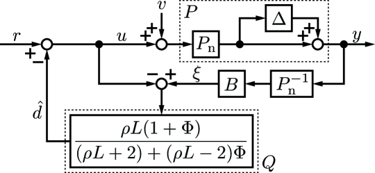
(a)

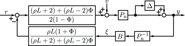
(b)

Figure 1: Block diagrams of the QDOB. (a) Disturbance-observer representation. (b) Equivalent single feedback-loop representation.

II-B Quasi-periodic Disturbance

Let a disturbance such that $d(t)=d(t-L)$ be periodic with a period $L\in\mathbb{R}_{>0}$. The periodic disturbance can be expressed by the Fourier series as

$$d(t)=\frac{a_{0}}{2}+\sum_{n=1}^{\infty}a_{n}\cos{\left(\frac{2n\pi}{L}t\right)}+b_{n}\sin{\left(\frac{2n\pi}{L}t\right)},$$ (7)

where, for a given $n$, the sum of the sine and cosine functions $a_{n}\cos{((2n\pi/L)t)}+b_{n}\sin{((2n\pi/L)t)}$ and the angular frequency $2n\pi/L$ are referred to as the $n$th harmonic and $n$th harmonic frequency, respectively.

This article expands the periodic disturbance into a quasi-periodic disturbance based on the definition of the quasi-periodicity in [26]. A lifted disturbance $D_{\tau}(c)$ of the disturbance $d(t)$ is defined as

$$D_{\tau}(c) \coloneqq d(t)\ \mathrm{s.t.}\ t=cL+\tau,$$ (8a)

$$D :\{\tau\in\mathbb{T}\}\times\{c\in\mathbb{Z}\}\to\mathbb{R},$$ (8b)

where $\mathbb{T}\coloneqq\{\tau\in\mathbb{R}_{\geq 0}|0\leq\tau<L\}$. The arguments $c$ and $\tau$ denote the cycle and the time elapsed within the cycle, respectively. Note that the lifted periodic disturbance satisfies $D_{\tau}(c)=D_{\tau}(c-1)$ for all cycles. Subsequently, in the frequency domain, let $\mathcal{D}_{\tau}(\omega)$ such that

$$\exists \omega\in\{\omega\in\mathbb{R}||\omega|\leq\rho\}\ \mathrm{s.t.}\ \mathcal{D}_{\tau}(\omega)\neq 0$$ (9a)

$$\forall \omega\in\{\omega\in\mathbb{R}||\omega|>\rho\}\ \mathrm{s.t.}\ \mathcal{D}_{\tau}(\omega)=0$$ (9b)

be quasi-periodic, where $\omega$ is the angular frequency and $\rho\in\mathbb{R}_{\geq 0}$ is referred to as the separation frequency. Using these, a set of functions of quasi-periodic disturbances is defined as follows:

$$\mathbb{P}_{\rho}\coloneqq\{d:\mathbb{R}\to\mathbb{R}| \eqref{eq:lifting}\land\eqref{eq:def:quasi-periodicity}\land D_{\tau}(c)=\mathcal{F}^{-1}[\mathcal{D}_{\tau}(\omega)],$$

$$\forall\tau\in\mathbb{T},\ \forall c\in\mathbb{Z},\ \forall\omega\in\mathbb{R}\},$$ (10)

and the disturbance $d(t)$ such that $d\in\mathbb{P}_{\rho}$ is defined to be quasi-periodic with respect to the separation frequency $\rho$. Here, $\mathcal{F}^{-1}$ denotes the inverse discrete-time Fourier transform. According to these definitions, the quasi-periodic disturbance has low-frequency changes and does not have high-frequency changes, in terms of the cycle $c$, where the boundary frequency between the low- and high-frequencies is the separation frequency $\rho$. Note that the quasi-periodic disturbance with respect to $\rho=0$ rad/s is equivalent to the periodic disturbance such that $d(t)=d(t-L)$.

II-C Q-filter

For the Q-filter of the QDOB (5), this article uses a periodic-pass filter of a first-order periodic/aperiodic separation filter proposed in [27, 26]. Since the lifted quasi-periodic disturbance $D_{\tau}(c)$ satisfies (9), it consists of low-frequency signals at frequencies less than or equal to the separation frequency $\rho$. Hence, a first-order low-pass filter, whose cutoff frequency is the separation frequency $\rho$, is used to extract the lifted quasi-periodic disturbance from the error $\Xi_{\tau}(c)-U_{\tau}(c)$ as

$$\frac{\mathcal{Z}[\hat{D}_{\tau}(c)]}{\mathcal{Z}[\Xi_{\tau}(c)-U_{\tau}(c)]}\coloneqq\frac{\rho L(1+Z^{-1})}{(\rho L+2)+(\rho L-2)Z^{-1}},$$ (11)

where $\hat{D}_{\tau}(c)$, $\Xi_{\tau}(c)$, and $U_{\tau}(c)$ are the lifted functions of $\hat{d}(t)$, $\xi(t)$, and $u(t)$, respectively. Note that the z-transform with $Z$ is based on the cycle $c$ with the sampling time $L$, which is the period of the cycle. The z-domain low-pass filter for the discrete-time lifted signals is transformed into an s-domain filter using the exact mapping $Z^{-1}=e^{-Ls}$ as

$$\frac{\mathcal{L}[\hat{d}]}{\mathcal{L}[\xi-u]}= \frac{\rho L(1+e^{-Ls})}{(\rho L+2)+(\rho L-2)e^{-Ls}},$$ (12)

which is the periodic-pass filter of the first-order periodic/aperiodic separation filter.

Although the time delays $e^{-Ls}$ of (12) are necessary for the quasi-periodic disturbance suppression, it induces amplification of aperiodic disturbances and deviation of harmonic suppression frequencies. Thus, a zero-phase low-pass filter is combined with the time delays to limit the frequencies, at which the time delay works. Consequently, the Q-filter of the QDOB is

$$Q(s) =\frac{\rho L(1+\Phi(s))}{(\rho L+2)+(\rho L-2)\Phi(s)},$$ (13)

where $\Phi(s)$ is the linear-phase low-pass filter, which is the product of the time delay and zero-phase low-pass filter. Fig. 2 depicts the Bode plot of the Q-filter (13) and the first-order periodic-pass filter (12), which shows that the effect of the time delay on the Q-filter is mitigated from around the cutoff frequency $\omega_{\mathrm{a}}=10\ \mathrm{rad/s}$.

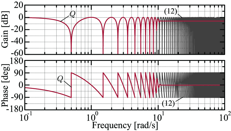
Figure 2: Bode plot of the Q-filter (13) of the QDOB and the first-order periodic-pass filter in (12). The parameters are $l=3$, $N_{\mathrm{max}}=256$, $\omega_{\mathrm{a}}=10\ \mathrm{rad/s}$, $\rho=2/L$, $L=2\pi\ \mathrm{s}$, and $T=1.0\times 10^{-4}\ \mathrm{s}$.

II-D Linear-Phase Low-Pass Filter

This section provides a design example of the linear-phase low-pass filter $\Phi(s)$ of the Q-filter (13). Prior to designing, $\Phi(s)$ is divided into a sample delay $e^{-Ts}$ of the sampling time $T\in\mathbb{R}_{>0}$ and a multistage linear-phase low-pass filter $\Psi(s)$ for implementation in discrete time

$$\Phi(s)=e^{-Ts}\Psi(s),\ \Psi(s)\coloneqq e^{(T-L)s}\prod_{i=1}^{l}H_{i}(s),$$ (14)

where $H_{i}(s)$ is the $i$th-stage zero-phase low-pass filter, and $l\in\mathbb{Z}_{>0}$ denotes the number of stages. A multistage design is employed here to realize a low cutoff frequency with less computational cost. The filter for each stage $H_{i}(s)$ is defined as

$$H_{i}(s)\coloneqq\frac{\sum_{n=-\infty}^{\infty}w(n,N)h(n,\omega_{i},U_{i})e^{nU_{i}s}}{\sum_{n=-\infty}^{\infty}w(n,N)h(n,\omega_{i},U_{i})}$$ (15a)

$$h(n,\omega_{i},U_{i})\coloneqq\left\{\begin{array}[]{cl}{U_{i}\omega_{i}}/{\pi}&\mathrm{if}\ n=0\\ {\sin(nU_{i}\omega_{i})}/{(n\pi)}&\mathrm{if}\ n\neq 0\\ \end{array}\right.$$ (15d)

$$w(n,N)\coloneqq\left\{\begin{array}[]{cl}\lx@intercol 0.42+0.5\cos({n\pi}{/N})\hfil\lx@intercol\\ +0.08\cos({2n\pi}/{N})&\mathrm{if}\ |n|\leq N\\ 0&\mathrm{if}\ |n|>N,\end{array}\right.$$ (15h)

where the coefficient $h(n,\omega_{i},U_{i})\in\mathbb{R}$ is derived by the inverse Fourier transform of the frequency characteristic of an ideal zero-phase low-pass filter, and the Blackman window $w(n,N)\in\mathbb{R}$ extracts a finite number of the coefficients. Multiplying $e^{(T-L)s}$ and $\prod_{i=1}^{l}H_{i}(s)$, the filter $\Psi(s)$ becomes

$$\Psi(s) =e^{(T-L+N\sum_{i=1}^{l}U_{i})s}\prod_{i=1}^{l}\varphi_{i}(s)$$ (16a)

$$\varphi_{i}(s) \coloneqq\frac{\sum_{n=-N}^{N}w(n,N)h(n,\omega_{i},U_{i})e^{(n-N)U_{i}s}}{\sum_{n=-N}^{N}w(n,N)h(n,\omega_{i},U_{i})},$$ (16b)

where the $i$th-stage sampling time $U_{i}\in\mathbb{R}_{>0}$, the $i$th-stage cutoff frequency $\omega_{i}\in\mathbb{R}_{>0}$, and the order $N\in\mathbb{R}_{>0}$ are determined as follows

$$U_{i} \coloneqq\left\{\begin{array}[]{cl}T&\mathrm{if}\ i=1\\ {\pi}/{\omega_{i-1}}&\mathrm{otherwise}\end{array}\right.$$ (17c)

$$\omega_{i} \coloneqq\left\{\begin{array}[]{cl}\omega_{\mathrm{a}}&\mathrm{if}\ i=l\\ {2c\pi}/{U_{i}}&\mathrm{otherwise},\end{array}\right.\ c=\frac{1}{2}\left(\frac{T\omega_{\mathrm{a}}}{\pi}\right)^{1/l}$$ (17f)

$$N \coloneqq\min\{\max(\mathcal{N}),\ N_{\mathrm{max}}\}$$ (17g)

$$\mathcal{N} \coloneqq\{n\in\mathbb{Z}_{>0}|n\leq(L-T)/\textstyle\sum_{j=1}^{i}U_{j}\}.$$ (17h)

The sampling time $U_{i}$ is set to the original sampling time $T$ for the first stage, while it is set for the other stages so that the $i$th-stage Nyquist frequency $\pi/U_{i}$ equals the cutoff frequency of the previous stage $\omega_{i-1}$. The cutoff frequency $\omega_{i}$ decreases over stages, and the coefficient $c$ is derived from the definitions of $U_{i}$ and $\omega_{i}$. The order $N$ is maximized in the set $\mathcal{N}$ of orders that make the filter $\Psi(s)$ causal, without exceeding the maximum order $N_{\mathrm{max}}$ given by allowed computational cost. Fig. 3 depicts the gain of the three-stage linear-phase low-pass filter $\Phi(s)$, in which one can see the reduction of the cutoff frequency stage-by-stage.

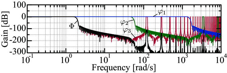
Figure 3: Gain of the three-stage linear-phase low-pass filter $\Phi(s)$ and the filters for each stage $\varphi_{1}$, $\varphi_{2}$, and $\varphi_{3}$. The parameters are $l=3$, $N_{\mathrm{max}}=256$, $\omega_{\mathrm{a}}=10\ \mathrm{rad/s}$, $L=2\pi\ \mathrm{s}$, and $T=1.0\times 10^{-4}\ \mathrm{s}$.

The linear-phase low-pass filter $\Phi(s)$ has three hyper parameters: the cutoff frequency $\omega_{\mathrm{a}}\in\mathbb{R}_{>0}$, the number of stages $l\in\mathbb{Z}_{>0}$, and the maximum order $N_{\mathrm{max}}\in\mathbb{Z}_{>0}$. The parameters $l$ and $N_{\mathrm{max}}$ are determined considering the trade-off that an increase in $l$ and/or $N_{\mathrm{max}}$ improves the filter $\Psi(s)$ to be closer to an ideal filter but increases the computational cost.

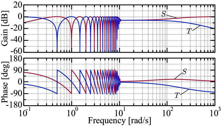
(a)

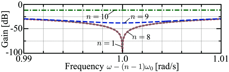
(b)

Figure 4: Bode plots of the sensitivity and complementary sensitivity functions in (19). The parameters are $l=3$, $N_{\mathrm{max}}=256$, $\omega_{\mathrm{a}}=10\ \mathrm{rad/s}$, $\omega_{\mathrm{b}}=100\ \mathrm{rad/s}$, $\rho=2/L$, $L=2\pi/\omega_{0}$, $\omega_{0}=1\ \mathrm{rad/s}$, and $T=1.0\times 10^{-4}\ \mathrm{s}$. (a) Sensitivity and complementary sensitivity functions. (b) Enlarged view of the gain of the sensitivity function at the $n$th harmonic frequencies.

III Design and Analysis

III-A Sensitivity and Complementary Sensitivity Functions

The cutoff frequencies $\omega_{\mathrm{a}}$ in (17f) and $\omega_{\mathrm{b}}$ in (6) are designed according to the sensitivity function (index for disturbance suppression) and complementary sensitivity function (index for robust stability and noise sensitivity). Suppose no modeling error $\Delta=0$. Then, the open-loop transfer function $\Gamma(s)$ is

$$\Gamma(s) =\frac{\rho L}{2}\frac{1+\Phi(s)}{1-\Phi(s)}B(s)=\frac{\rho L}{2}\frac{1+\Phi(s)}{1-\Phi(s)}\frac{\omega_{\mathrm{b}}}{s+\omega_{\mathrm{b}}}$$ (18)

according to Fig. 1(b). Using the open-loop transfer function, the sensitivity function $S(s)$ and the complementary sensitivity function $T(s)$ are defined and calculated as

$$S(s) \coloneqq\frac{1}{1+\Gamma}=\frac{2(1-\Phi)}{(\rho LB+2)+(\rho LB-2)\Phi}$$ (19a)

$$T(s) \coloneqq\frac{\Gamma}{1+\Gamma}=\frac{\rho L(1+\Phi)B}{(\rho LB+2)+(\rho LB-2)\Phi}.$$ (19b)

The sensitivity function satisfies $\mathcal{L}[y]/\mathcal{L}[d]=P_{\mathrm{n}}(s)S(s)$.

The sensitivity and complementary sensitivity functions show different features in the three frequency ranges: $0\leq\omega\ll\omega_{\mathrm{a}}$, $\omega_{\mathrm{a}}\ll\omega\ll\omega_{\mathrm{b}}$, and $\omega_{\mathrm{b}}\ll\omega\ll 2\pi/T$, as shown in Fig. 4(a). Note that $2\pi/T$ stands for the sampling frequency. In each range, the transfer functions can be approximated as follows

$$0\leq\omega\ll\omega_{\mathrm{a}}:$$

$$S(j\omega)\approx\frac{2(1-e^{-jL\omega})}{(\rho L+2)+(\rho L-2)e^{-jL\omega}}$$ (20a)

$$T(j\omega)\approx\frac{\rho L(1+e^{-jL\omega})}{(\rho L+2)+(\rho L-2)e^{-jL\omega}}$$ (20b)

$$\omega_{\mathrm{a}}\ll\omega\ll\omega_{\mathrm{b}}:$$

$$S(j\omega)\approx\frac{2}{\rho L+2},\ T(j\omega)\approx\frac{\rho L}{\rho L+2}$$ (20c)

$$\omega_{\mathrm{b}}\ll\omega\ll 2\pi/T:$$

$$S(j\omega)\approx\frac{2}{\rho LB(j\omega)+2},\ T(j\omega)\approx\frac{\rho LB(j\omega)}{\rho LB(j\omega)+2},$$ (20d)

which are based on the approximation of the low-pass filters: $\Phi(j\omega)\approx 1$ if $\omega\ll\omega_{\mathrm{a}}$; $\Phi(j\omega)\approx 0$ if $\omega_{\mathrm{a}}\ll\omega\ll 2\pi/T$; and $B(j\omega)\approx 1$ if $\omega\ll\omega_{\mathrm{b}}$. The lower-frequency range $\omega\ll\omega_{\mathrm{a}}$ is the range relevant to the quasi-periodic disturbance suppression, where the sensitivity function $S(s)$ becomes the periodic-pass filter (12). In the higher-frequency range $\omega_{\mathrm{b}}\ll\omega\ll 2\pi/T$, the low-pass filter $B(s)$ becomes dominant for the low noise sensitivity and high robust stability via the complementary sensitivity function $T(s)$. Lastly, the middle-frequency range $\omega_{\mathrm{a}}\ll\omega\ll\omega_{\mathrm{b}}$, which separates the higher- and lower-frequency ranges, rejects the amplification of aperiodic disturbances and the deviation of the harmonic suppression frequencies, which can be observed in Fig. 4(a) and Fig. 4(b), respectively.

Therefore, the cutoff frequency $\omega_{\mathrm{a}}$ is designed to be higher than the target harmonic frequencies $\omega_{0},\ 2\omega_{0},\ 3\omega_{0},\ \ldots$ to be compensated and lower than the other cutoff frequency $\omega_{\mathrm{b}}$.

III-B Harmonic Suppression Bandwidth

The suppression bandwidth around the harmonics is designed via the separation frequency $\rho$ of the Q-filter (13). Considering the approximate sensitivity function (20a) in the frequency range $0\leq\omega\ll\omega_{\mathrm{a}}$, the gain is

$$\left|\frac{2(1-e^{-Ls})}{(\rho L+2)+(\rho L-2)e^{-Ls}}\right|=\sqrt{\frac{4\tan^{2}(L\omega/2)}{\rho^{2}L^{2}+4\tan^{2}(L\omega/2)}}.$$ (21)

By determining the separation frequency as

$$\rho\coloneqq\frac{2}{L}\tan{\left(\frac{L}{2}\omega_{\mathrm{c}}\right)},$$ (22)

the gain of the sensitivity function satisfies

$$20\log|S(j(n\omega_{0}\pm\omega_{\mathrm{c}}))|\approx-3\ \mathrm{dB},$$ (23)

where $\omega_{\mathrm{c}}\in\{\omega\in\mathbb{R}_{>0}|0<\omega<\omega_{0}/2\}$ is also referred to as the cutoff frequency. The harmonic suppression bandwidth is from $n\omega_{0}-\omega_{\mathrm{c}}$ to $n\omega_{0}+\omega_{\mathrm{c}}$ around a harmonic frequency $n\omega_{0}$, in which the gain is less than $-3\ \mathrm{dB}$; thus, an increase in the cutoff frequency $\omega_{\mathrm{c}}$ achieves wideband harmonic suppression. Fig. 5 shows that (23) holds with various cutoff frequencies from the first harmonic to the seventh harmonic frequency.

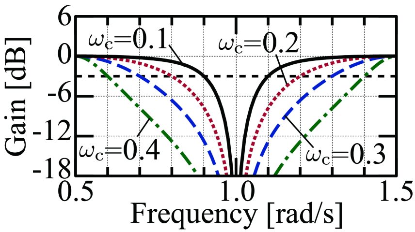
(a) First harmonic.

(b) Third harmonic.

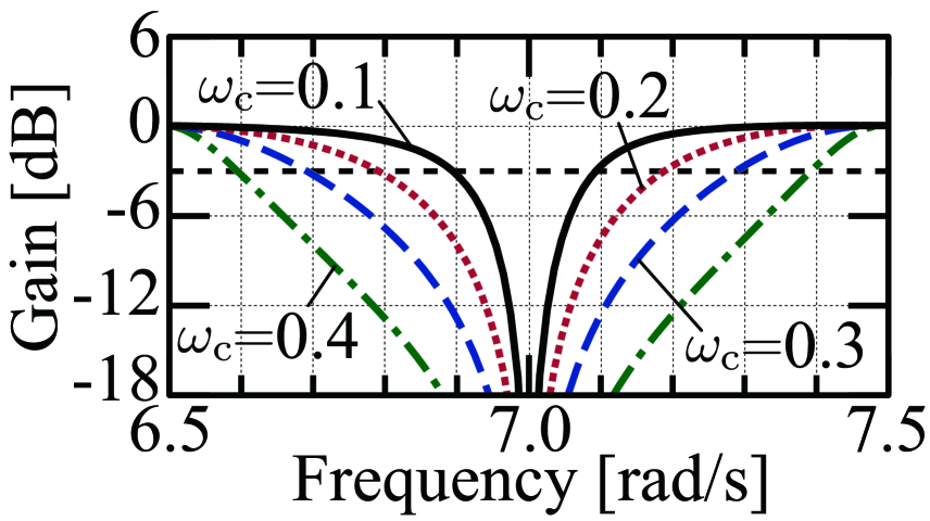
(c) Fifth harmonic.

(d) Seventh harmonic.

Figure 5: Bode plots of the sensitivity function in (19a) with the design of the separation frequency $\rho$ in (22) and the various cutoff frequencies $\omega_{\mathrm{c}}$. The parameters are $l=3$, $N_{\mathrm{max}}=256$, $\omega_{\mathrm{a}}=10\ \mathrm{rad/s}$, $\omega_{\mathrm{b}}=100\ \mathrm{rad/s}$, $L=2\pi/\omega_{0}$, $\omega_{0}=1\ \mathrm{rad/s}$, and $T=1.0\times 10^{-4}\ \mathrm{s}$.

III-C Nominal Stability

Consider the nominal stability with a stable plant model $P_{\mathrm{n}}(s)$ whose poles are in the open left half-plane in the complex plane. In the open-loop transfer function (18), the phase of the first-order low-pass filter $B(s)$ satisfies

$$-\pi/2<\angle B(j\omega)=\mathrm{atan}2({-\omega,\ \omega_{\mathrm{b}}})\leq 0,\ \forall\omega\in\mathbb{R}_{\geq 0}.$$ (24)

Using the linear phase characteristic $\Phi(j\omega)=|\Phi(j\omega)|e^{-jL\omega}$ of $\Phi(s)$, the phase of the other part is expressed as

$$\angle\frac{\rho L}{2}\frac{1+|\Phi(j\omega)|e^{-jL\omega}}{1-|\Phi(j\omega)|e^{-jL\omega}}$$

$$\hskip 10.00002pt=\angle\frac{\rho L}{2}\dfrac{(1-|\Phi(j\omega)|^{2})-j2|\Phi(j\omega)|\sin(L\omega)}{1-2|\Phi(j\omega)|\cos(L\omega)+|\Phi(j\omega)|^{2}}$$

$$\hskip 10.00002pt=\mathrm{atan}2({-2|\Phi(j\omega)|\sin(L\omega),\ 1-|\Phi(j\omega)|^{2}}).$$ (25)

Assume that the gain of the linear phase low-pass filter satisfies $|\Phi(j\omega)|\leq 1$, which is practical according to Fig. 3. Then, $1-|\Phi(j\omega)|^{2}$ is nonnegative, and the phase satisfies

$$-\frac{\pi}{2}\leq\angle\left(\frac{\rho L}{2}\dfrac{1+\Phi(j\omega)}{1-\Phi(j\omega)}\right)\leq\frac{\pi}{2},\ \forall\omega\in\mathbb{R}_{\geq 0}.$$ (26)

According to (24) and (26), the overall phase of the open-loop transfer function (18) exists within

$$-\pi<\angle\Gamma(j\omega)\leq\frac{\pi}{2},\ \forall\omega\in\mathbb{R}_{\geq 0}$$ (27)

and does not reach $-\pi$ rad/s. On the basis of the Nyquist stability criteria, the system is nominally stable.

The stability margin is extended by designing the cutoff frequencies $\omega_{\mathrm{a}}$ and $\omega_{\mathrm{b}}$ so that $\omega_{\mathrm{a}}\ll\omega_{\mathrm{b}}$, as described in Section III-A. Satisfying $\omega_{\mathrm{a}}\ll\omega_{\mathrm{b}}$, the phase range narrows to approximately $-\pi/2\leq\angle\Gamma(j\omega)\leq\pi/2$, and a phase margin of $-\pi/2$ rad is secured within a frequency range less than the sampling frequency, as shown in the phase plot of Fig. 6. Additionally, the low-pass filter $B(s)$ extends the gain margin at frequencies greater than $\omega_{\mathrm{b}}$, as shown in the gain plot of Fig. 6.

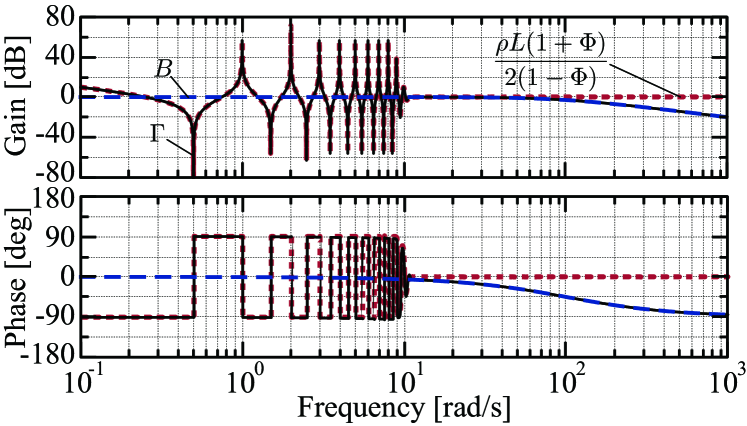
Figure 6: Bode plot of the open-loop transfer function. The parameters are $l=3$, $N_{\mathrm{max}}=256$, $\omega_{\mathrm{a}}=10\ \mathrm{rad/s}$, $\omega_{\mathrm{b}}=100\ \mathrm{rad/s}$, $\rho=2/L$, $L=2\pi/\omega_{0}$, $\omega_{0}=1\ \mathrm{rad/s}$, and $T=1.0\times 10^{-4}\ \mathrm{s}$.

III-D Robust Stability

Consider the robust stability against the modeling error $\Delta(s)$. Let $\tilde{T}(s)$ be

$$\tilde{T}(s)\coloneqq\left\{\begin{array}[]{cl}\dfrac{\rho L(1+e^{-Ls})}{(\rho L+2)+(\rho L-2)e^{-Ls}}&\mathrm{if}\ \omega\leq\omega_{\mathrm{a}}\\ \dfrac{\rho LB(s)}{\rho LB(s)+2}&\mathrm{if}\ \omega>\omega_{\mathrm{a}},\end{array}\right.$$ (30)

which is the right-hand side of (20). Then, the complementary sensitivity function $T$ is decomposed into $T(s)=\sigma(s)\tilde{T}(s)$, where $\sigma(s)$ is the approximation error of (20). Note that the approximation error $\sigma(s)$ decreases as $\omega_{\mathrm{b}}$ increases relative to $\omega_{\mathrm{a}}$. Let the worst error $\tilde{\Delta}(s)$ be known such that $|\sigma(j\omega)\Delta(j\omega)|<\tilde{\Delta}(\omega),\ \forall\omega\in\mathbb{R}_{\geq 0}$ against both the modeling error $\Delta(j\omega)$ and approximation error $\sigma(j\omega)$.

Suppose the system is nominally stable on the basis of Section III-C. Then, the robust stability condition based on the small gain theorem is

$$|\tilde{T}(j\omega)|\leq\tilde{\Delta}^{-1}(\omega),\ \forall\omega\in\mathbb{R}_{\geq 0}.$$ (31)

The gain of $\tilde{T}$ can be calculated as

$$|\tilde{T}(j\omega)| =\frac{\rho L}{\sqrt{\rho^{2}L^{2}+4\tan^{2}(L\omega/2)}},\ \mathrm{if}\ \omega\leq\omega_{\mathrm{a}}$$ (32a)

$$|\tilde{T}(j\omega)| =\frac{\rho L\omega_{\mathrm{b}}}{\sqrt{4\omega^{2}+(2+\rho L)^{2}\omega_{\mathrm{b}}^{2}}},\ \mathrm{if}\ \omega>\omega_{\mathrm{a}},$$ (32b)

where the gain (32a) at $\omega\leq\omega_{\mathrm{a}}$ is less than or equal to 1, and the gain (32b) at $\omega>\omega_{\mathrm{a}}$ decreases as $\omega_{\mathrm{a}}$ and/or $\rho$ decreases.

Suppose that the separation frequency $\rho$ is designed by (22) with the cutoff frequency $\omega_{\mathrm{c}}$, and the other cutoff frequencies satisfy $\omega_{\mathrm{a}}\ll\omega_{\mathrm{b}}$ according to Section III-A. Then, for the robust stability of the QDOB, the cutoff frequencies $\omega_{\mathrm{b}}$ and $\omega_{\mathrm{c}}$ need to be low enough to satisfy the condition (31).

Algorithm 1 Algorithm of QDOB for motion control.

Hyperparameters:
       $\mu\in\{0,1\}$, $l$, $N_{\mathrm{max}}\in\mathbb{Z}_{>0}$, $\omega_{\mathrm{a}}$, $\omega_{\mathrm{b}}$, $\omega_{\mathrm{c}}$, $L$, $M$, $T\in\mathbb{R}_{>0}$
Preliminary computations:

$$\rho=(2/L)\tan{\left(L\omega_{\mathrm{c}}/2\right)}$$

$$\bar{L}=\mathrm{round}({L/T})$$

$$c=(1/2)(T\omega_{\mathrm{a}}/\pi)^{1/l}$$

$$\bm{\mathrm{for}}\ i=1\ \ldots\ l\ \bm{\mathrm{do}}$$

$$\hskip 20.00003pt\bm{\mathrm{if}}\ i==1\ \bm{\mathrm{then}}$$

$$\hskip 20.00003pt\hskip 20.00003ptU_{i}=T$$

$$\hskip 20.00003pt\bm{\mathrm{else}}$$

$$\hskip 20.00003pt\hskip 20.00003ptU_{i}=\pi/\omega_{i-1}$$

$$\hskip 20.00003pt\bm{\mathrm{end\ if}}$$

$$\hskip 20.00003pt\bar{U}_{i}=\mathrm{round}({U_{i}/T})$$

$$\hskip 20.00003pt\omega_{i}={2\pi c}/{U_{i}}$$

$$\bm{\mathrm{end\ for}}$$

$$N=\min\{\mathrm{floor}((\bar{L}-1)/\textstyle\sum_{i=1}^{l}\bar{U}_{i}),\ N_{\mathrm{max}}\}$$

$$\eta=\bar{L}-N\textstyle\sum_{i=1}^{l}\bar{U}_{i}$$

Function $\mathcal{P}(\lambda_{k-1})$:
      Sub-functions:

$$h(n,\omega_{i},U_{i})=\left\{\begin{array}[]{cl}{U_{i}\omega_{i}}/{\pi}&\mathrm{if}\ n=0\\ {\sin(nU_{i}\omega_{i})}/{(n\pi)}&\mathrm{if}\ n\neq 0\\ \end{array}\right.$$

$$w(n,N)=0.42+0.5\cos({n\pi}{/N})+0.08\cos({2n\pi}/{N})$$

Input: $\lambda_{k-1}$,  Output: $\!\!\mbox{ }^{l}\theta_{k}$

$$\!\!\mbox{ }^{0}\theta_{k}=\lambda_{k-\eta}$$

$$\bm{\mathrm{for}}\ i=1\ \ldots\ l\ \bm{\mathrm{do}}$$

$$\hskip 20.00003pt\bm{\mathrm{for}}\ n=-N\ \ldots\ N\ \bm{\mathrm{do}}$$

$$\hskip 40.00006pt\!\!\mbox{ }^{i}\theta_{k}\mathrel{+}=w(n,N)h(n,\omega_{i},U_{i})\ \!\!\mbox{ }^{i-1}\theta_{k+(n-N)\bar{U}_{i}}$$

$$\hskip 40.00006pt\!\!\mbox{ }^{i}\gamma_{k}\mathrel{+}=w(n,N)h(n,\omega_{i},U_{i})$$

$$\hskip 20.00003pt\bm{\mathrm{end\ for}}$$

$$\hskip 20.00003pt\!\!\mbox{ }^{i}\theta_{k}=\!\!\mbox{ }^{i}\theta_{k}/\!\!\mbox{ }^{i}\gamma_{k}$$

$$\bm{\mathrm{end\ for}}$$

Real-time algorithm
      Inputs: Reference ${r}_{k}$, Position response $y_{k}$
      Output: Control input $u_{k}$, Estimated disturbance $\hat{d}_{k}$

$$\xi_{k}=\frac{1}{T(1+\omega_{\mathrm{b}}T)}[T\xi_{k-1}+M\omega_{\mathrm{b}}(y_{k}-2y_{k-1}+y_{k-2})]$$

$$\hat{d}_{k}=\frac{\rho L}{(1-\mu)\rho L+2}(\xi_{k}-r_{k})+\mathcal{P}(\lambda_{k-1})$$

$$\lambda_{k}=\frac{\rho L}{(1-\mu)\rho L+2}(\xi_{k}-r_{k})-\frac{(1-\mu)\rho L-2}{(1-\mu)\rho L+2}\hat{d}_{k}$$

$$u_{k}=r_{k}-\mu\hat{d}_{k}$$

IV Discretization

Let us discretize the QDOB for motion control of a mechanical system, whose plant model is

$$P_{\mathrm{n}}(s)=\frac{1}{Ms^{2}}.$$ (33)

The inverse plant model is $P_{\mathrm{n}}^{-1}(s)=Ms^{2}$.

The QDOB is discretized using two methods. The inverse plant model $P_{\mathrm{n}}^{-1}(s)$ and the low-pass filter $B(s)$ in (6) are discretized by the backward Euler method: $s\leftarrow(1-z^{-1})/T$ as

$$\mathcal{Z}[\xi_{k}]=\frac{M\omega_{\mathrm{b}}(1-z^{-1})^{2}}{T(1+\omega_{\mathrm{b}}T-z^{-1})}\mathcal{Z}[y_{k}].$$ (34)

Subsequently, the Q-filter in (13) is discretized by the exact mapping from the s-plane to the z-plane: $e^{-Ts}\leftarrow z^{-1}$ as

$$\mathcal{Z}[\hat{d}_{k}]=\frac{\rho L(1+\bar{\Psi}(z^{-1})z^{-1})}{(\rho L+2)+(\rho L-2)\bar{\Psi}(z^{-1})z^{-1}}\mathcal{Z}[\xi_{k}-u_{k}]$$ (35a)

$$\bar{\Psi}(z^{-1})\coloneqq z^{1-\bar{L}+N\sum_{i=0}^{l}\bar{U}_{i}}\prod_{i=0}^{l}\bar{\varphi}_{i}(z^{-1})$$ (35b)

$$\bar{\varphi}_{i}(z^{-1})\coloneqq\frac{\sum_{n=-N}^{N}w(n,N)h(n,\omega_{i},U_{i})z^{(n-N)\bar{U}_{i}}}{\sum_{n=-N}^{N}w(n,N)h(n,\omega_{i},U_{i})},$$ (35c)

where $\bar{L}_{i}\coloneqq\mathrm{round}({L_{i}/T})$ and $\bar{U}_{i}\coloneqq\mathrm{round}({U_{i}/T})$. This z-transform with $z$ is based on the index $k$ with the sampling time $T$ from the controller.

Algorithm 1 shows the whole discrete-time algorithm of a discrete-time representation of the QDOB. The discrete-time representation of (34) is obtained by the inverse z-transform as

$$\xi_{k} =\frac{T\xi_{k-1}+M\omega_{\mathrm{b}}(y_{k}-2y_{k-1}+y_{k-2})}{T(1+\omega_{\mathrm{b}}T)}.$$ (36)

The Q-filter (35a) is transformed for gathering the linear-phase low-pass filter $\bar{\Psi}(z^{-1})$ to reduce the number of buffers into

$$\mathcal{Z}[\hat{d}_{k}] =\frac{\rho L}{\rho L+2}\mathcal{Z}[\xi_{k}-u_{k}]+\bar{\Psi}(z^{-1})$$

$$\left(\frac{\rho L}{\rho L+2}\mathcal{Z}[\xi_{k-1}-u_{k-1}]-\frac{\rho L-2}{\rho L+2}\mathcal{Z}[\hat{d}_{k-1}]\right).$$ (37)

The inverse z-transform and $u_{k}=r_{k}-\mu\hat{d}_{k}$ yields its discrete-time representation:

$$\hat{d}_{k}=\frac{\rho L}{(1-\mu)\rho L+2}(\xi_{k}-r_{k})+\mathcal{P}(\lambda_{k-1})$$ (38a)

$$\mathcal{P}(\lambda_{k-1})\coloneqq\mathcal{Z}^{-1}[\bar{\Psi}(z^{-1})\mathcal{Z}[\lambda_{k-1}]]$$ (38b)

$$\lambda_{k}\coloneqq\frac{\rho L}{(1-\mu)\rho L+2}(\xi_{k}-r_{k})-\frac{(1-\mu)\rho L-2}{(1-\mu)\rho L+2}\hat{d}_{k},$$ (38c)

where a new parameter $\mu\in\{0,1\}$ is introduced for switching between estimation use with $\mu=0$ and compensation use with $\mu=1$. These discrete-time representations are listed in Algorithm 1 along with the hyperparameters, preliminary computations of the parameters, and the algorithm of the function (38b).

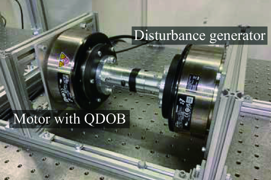
(a)

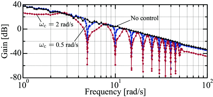
(b)

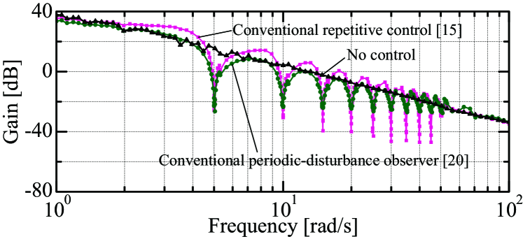
(c)

Figure 7: Frequency-response experiment. (a) Setup. (b) Results of the QDOB. (c) Results of the conventional methods [15] and [20].

V Experiments

V-A Frequency Response

The frequency response with the QDOB from the external torque $v$ to the angle $y$ was validated and compared with those of the conventional repetitive control [15] and periodic-disturbance observer [20]. Two direct-drive motors connected by a coupling were used, as shown in Fig. 7(a), where the left motor is controlled by the QDOB, and the right motor generated external torque $v=a_{\mathrm{v}}\sin(\omega_{\mathrm{v}}t)$. During the experiment, the frequency $\omega_{\mathrm{v}}$ was varied from $10^{0}$ to $10^{2}$ rad/s, and the amplitude $a_{\mathrm{v}}$ was set not to exceed the actuators’ angle, velocity, and torque limits. Each sinusoidal response was tested for 40 or 60 s, and the discrete-time Fourier transform was applied to the steady-state response, eliminating the initial 20-s transient response to compute the gain. The QDOB used the parameters: $l=3$, $N_{\mathrm{max}}=256$, $\omega_{\mathrm{a}}=50$ rad/s, $\omega_{\mathrm{b}}=100$ rad/s, $\omega_{\mathrm{c}}\in\{0.5,\ 2\}$ rad/s, $M=56.13\times 10^{-4}$ $\mathrm{kg\!\cdot\!m^{2}}$, $L=2\pi/5$ s, and $T=2\times 10^{-4}$ s. The conventional repetitive control used the same zero-phase low-pass filter as that of the QDOB with $\alpha=0.9$. Also, in the conventional periodic-disturbance observer, the Q-filter used $\gamma=0.5$ and the cutoff frequency $g=50$ rad/s, and the pseudo-differentiation used the cutoff frequency 100 rad/s.

Fig. 7(b) depicts the three frequency responses: without control, with the QDOB using $\omega_{\mathrm{c}}=0.5$ rad/s, and with the QDOB using $\omega_{\mathrm{c}}=2$ rad/s. The frequency response without control showed that the plant was a second-order system, and the effect of the QDOB appeared as the difference from this frequency response. The frequency response with the QDOB realized sharp band-stop frequencies at the harmonic frequencies from the first harmonic of 5 rad/s to the tenth harmonic of 50 rad/s. These target harmonic frequencies were determined by the cutoff frequency $\omega_{\mathrm{a}}$ of 50 rad/s. Compared to the cutoff frequency $\omega_{\mathrm{c}}=0.5$ rad/s, $\omega_{\mathrm{c}}=2$ rad/s extended the suppression bandwidth around the harmonic frequencies without amplification of aperiodic disturbances and deviation of harmonic suppression frequencies. From 60 rad/s to 100 rad/s, the gain decreased on the basis of (20c), where the gain decreases as the the cutoff frequency $\omega_{\mathrm{c}}$ increases.

The proposed QDOB was compared with the conventional methods in Fig. 7(c). The conventional repetitive control [15] showed aperiodic disturbance amplification caused by the trade-off between the wideband suppression and the amplification. The conventional periodic-disturbance observer [20] showed wider suppression around the harmonics and non-amplification of the aperiodic disturbances from 1 to 35 rad/s; however, the harmonic suppression performance was less than that of the repetitive control, the amplification appeared from 35 rad/s, and the high-order harmonic suppression frequencies deviated slightly. Compared to them, the QDOB achieved lower gain at the harmonic frequencies (5, 10, 15, $\ldots$, 45 rad/s), wideband suppression around the harmonic frequencies with $\omega_{\mathrm{c}}=0.5$ rad/s, non-amplification around the aperiodic-disturbance frequencies (2.5, 7.5, 12.5, $\ldots$, 47.5 rad/s), and non-deviation of the harmonic suppression frequencies, as shown in Fig. 7(b). The lower gain of the QDOB at the harmonic frequencies was caused by the zero-phase low-pass filter integrated with each time delay.

V-B Manipulator Control

The QDOB was used to control the six-degree-of-freedom manipulator (Fig. 8(a)) with proportional-and-derivative angle control and feedforward control in the joint space. The effect of the QDOB was verified and compared with a conventional disturbance observer [19]. The outer joint-space proportional-and-derivative controller was

$$\dot{\hat{\bm{e}}}(t) =\bm{G}(\bm{e}(t)-\hat{\bm{e}}(t)),\ \bm{e}(t)=\bm{\theta}^{\mathrm{cmd}}(t)-\bm{\theta}(t)$$ (39a)

$$\ddot{\hat{\bm{\theta}}}^{\mathrm{cmd}}(t) =\bm{G}^{2}\bm{\theta}^{\mathrm{cmd}}(t)-2\bm{G}\dot{\hat{\bm{\theta}}}^{\mathrm{cmd}}(t)-\bm{G}^{2}\hat{\bm{\theta}}^{\mathrm{cmd}}(t)$$ (39b)

$$\bm{r}(t) =\bm{K}_{\mathrm{p}}\bm{e}(t)+\bm{K}_{\mathrm{d}}\dot{\hat{\bm{e}}}(t)+\bm{M}\ddot{\hat{\bm{\theta}}}^{\mathrm{cmd}}(t),$$ (39c)

where the derivative gain, proportional gain, moment of inertia matrix, and cutoff frequency for the pseudo-differentiation were set as $\bm{K}_{\mathrm{d}}=\bm{\mathrm{diag}}$(0.5, 0.5, 0.4, 0.1, 0.05, 0.05) $\mathrm{N\!\cdot\!m\!\cdot\!s}/\mathrm{rad}$, $\bm{K}_{\mathrm{p}}=\bm{\mathrm{diag}}$(3, 3, 1.5, 0.5, 0.2, 0.2) $\mathrm{N\!\cdot\!m}/\mathrm{rad}$, $\bm{M}=\bm{\mathrm{diag}}$(8, 30, 20, 0.5, 1, 0.1)$\times 10^{-3}$ $\mathrm{kg\!\cdot\!m^{2}}$, and $\bm{G}=\bm{\mathrm{diag}}$(200, 200, 200, 200, 200, 100) rad/s, respectively. The variables $\bm{\theta}^{\mathrm{cmd}}(t)\in\mathbb{R}^{6}$, $\bm{\theta}(t)\in\mathbb{R}^{6}$, and $\bm{e}(t)\in\mathbb{R}^{6}$ denote the command angle, response angle, and angle error, respectively. The QDOB used the same parameters as those in Section V-A, except for the cutoff frequency $\omega_{\mathrm{c}}=2$ rad/s, period $L=4$ s, and sampling time $T=2\times 10^{-3}$ s. The conventional disturbance observer used the cutoff frequency of 50 rad/s for its Q-filter. The manipulator was position controlled with periodic position and orientation commands for the end-effector with the period of four seconds, where there were periodic disturbances such as gravity and friction.

The command and response waveforms from 0 s to 50 s of the end-effector position (x-y-z) and orientation (roll-pitch-yaw) with the QDOB are depicted in Fig. 8(b) and (d), respectively. They show that the QDOB needed almost four cycles (16 s) of the 4-s period to be effective, owing to the buffer implementing the linear-phase low-pass filter. The discrete-time Fourier transform was applied to the steady-state errors of the position and orientation from 30 s to 180 s for both the QDOB and the conventional disturbance observer [19]. Fig. 8(c) shows the sum of the amplitudes of the Fourier transformed position errors, and Fig. 8(e) shows that of the Fourier transformed orientation errors. The harmonic suppression of the QDOB from the first harmonic (1.571 rad/s) to the ninth harmonic (14.137 rad/s) was observed for both position and orientation, compared to the conventional disturbance observer.

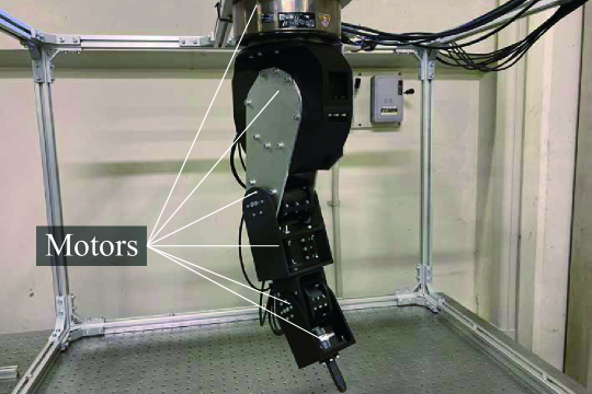
(a)

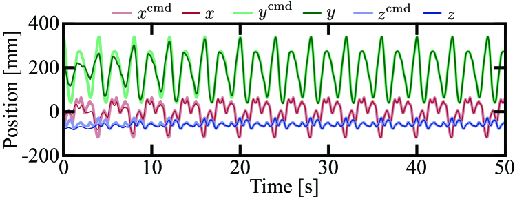
(b)

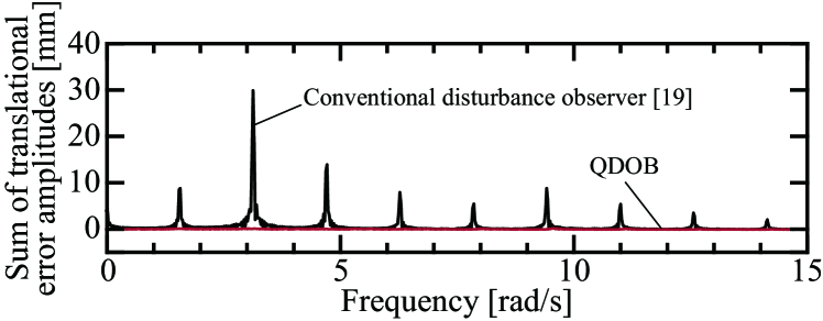
(c)

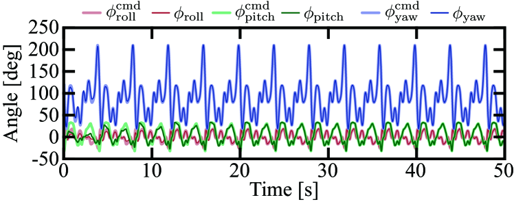
(d)

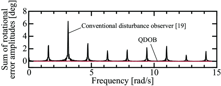
(e)

Figure 8: Manipulator-control experiment. (a) Setup. (b) Position (x-y-z) results of the QDOB. (c) Sum of the amplitudes of the discrete-time Fourier transformed translational errors in the steady state. (d) Orientation (roll-pitch-yaw) results of the QDOB. (e) Sum of the amplitudes of the discrete-time Fourier transformed rotational errors in the steady state.

VI Conclusion

This paper proposed the QDOB to estimate and compensate for quasi-periodic disturbances. The QDOB has three cutoff frequencies $\omega_{\mathrm{a}}$, $\omega_{\mathrm{b}}$, and $\omega_{\mathrm{c}}$, such that $\omega_{\mathrm{a}}\ll\omega_{\mathrm{b}}$. The harmonics with frequencies lower than $\omega_{\mathrm{a}}$ are compensated, and the robust stability can be improved by lowering $\omega_{\mathrm{b}}$ and $\omega_{\mathrm{c}}$. For wideband harmonic suppression, increasing $\omega_{\mathrm{c}}$ extends the suppression bandwidth around harmonics without amplifying aperiodic disturbances and deviating the harmonic suppression frequencies.

Hisayoshi Muramatsu Hisayoshi Muramatsu received the B.E. degree in system design engineering and the M.E. and Ph.D. degrees in integrated design engineering from Keio University, Yokohama, Japan, in 2016, 2017, and 2020, respectively. From 2019 to 2020, he was a Research Fellow with the Japan Society for the Promotion of Science. He is currently an Assistant Professor with the Mechanical Engineering Program, Hiroshima University, Higashihiroshima, Japan. His research interests include motion control, robotics, and physical human-robot interaction.

References

- [1] I. Houtzager, J.-W. van Wingerden, and M. Verhaegen, “Rejection of periodic wind disturbances on a smart rotor test section using lifted repetitive control,” IEEE Trans. Control Syst. Technol., vol. 21, no. 2, pp. 347–359, Mar. 2013.
- [2] H. Fujimoto and T. Takemura, “High-precision control of ball-screw-driven stage based on repetitive control using -times learning filter,” IEEE Trans. Ind. Electron., vol. 61, no. 7, pp. 3694–3703, Jul. 2014.
- [3] M. Tang, A. Formentini, S. A. Odhano, and P. Zanchetta, “Torque ripple reduction of pmsms using a novel angle-based repetitive observer,” IEEE Trans. Ind. Electron., vol. 67, no. 4, pp. 2689–2699, Apr. 2020.
- [4] Z. Wang, J. Zhao, L. Wang, M. Li, and Y. Hu, “Combined vector resonant and active disturbance rejection control for PMSLM current harmonic suppression,” IEEE Trans. Ind. Informat., vol. 16, no. 9, pp. 5691–5702, Sep. 2020.
- [5] G. Liu, B. Chen, K. Wang, and X. Song, “Selective current harmonic suppression for high-speed PMSM based on high-precision harmonic detection method,” IEEE Trans. Ind. Informat., vol. 15, no. 6, pp. 3457–3468, Jun. 2019.
- [6] G. Li, G. Tang, and X. Liu, “An internal voltage robust control of battery energy storage system for suppressing wideband harmonics in vf control-based islanded microgrids,” IEEE Trans. Ind. Informat., vol. 20, no. 2, pp. 2320–2330, Feb. 2024.
- [7] H. Patel and V. Agarwal, “Control of a stand-alone inverter-based distributed generation source for voltage regulation and harmonic compensation,” IEEE Trans. Power Del., vol. 23, no. 2, pp. 1113–1120, Apr. 2008.
- [8] S. Hara, Y. Yamamoto, T. Omata, and M. Nakano, “Repetitive control system: a new type servo system for periodic exogenous signals,” IEEE Trans. Autom. Control, vol. 33, no. 7, pp. 659–668, Jul. 1988.
- [9] Y. Wang, F. Gao, and F. J. Doyle, “Survey on iterative learning control, repetitive control, and run-to-run control,” Journal of Process Control, vol. 19, no. 10, pp. 1589 – 1600, Dec. 2009.
- [10] D. A. Bristow, M. Tharayil, and A. G. Alleyne, “A survey of iterative learning control,” IEEE Control Systems Magazine, vol. 26, no. 3, pp. 96–114, Jun. 2006.
- [11] N. Mooren, G. Witvoet, and T. Oomen, “Gaussian process repetitive control: Beyond periodic internal models through kernels,” Automatica, vol. 140, p. 110273, Jun. 2022.
- [12] M. Steinbuch, “Repetitive control for systems with uncertain period-time,” Automatica, vol. 38, no. 12, pp. 2103–2109, Dec. 2002.
- [13] M. Steinbuch, S. Weiland, and T. Singh, “Design of noise and period-time robust high-order repetitive control, with application to optical storage,” Automatica, vol. 43, no. 12, pp. 2086–2095, Dec. 2007.
- [14] G. Pipeleers, B. Demeulenaere, J. De Schutter, and J. Swevers, “Robust high-order repetitive control: Optimal performance trade-offs,” Automatica, vol. 44, no. 10, pp. 2628–2634, Oct. 2008.
- [15] X. Chen and M. Tomizuka, “New repetitive control with improved steady-state performance and accelerated transient,” IEEE Trans. Control Syst. Technol., vol. 22, no. 2, pp. 664–675, Mar. 2014.
- [16] K. Nie, W. Xue, C. Zhang, and Y. Mao, “Disturbance observer-based repetitive control with application to optoelectronic precision positioning system,” J. Franklin Inst., vol. 358, no. 16, pp. 8443–8469, Oct. 2021.
- [17] E. Sariyildiz, R. Oboe, and K. Ohnishi, “Disturbance observer-based robust control and its applications: 35th anniversary overview,” IEEE Trans. Ind. Electron., vol. 67, no. 3, pp. 2042–2053, Mar. 2020.
- [18] W. H. Chen, J. Yang, L. Guo, and S. Li, “Disturbance-observer-based control and related methods–an overview,” IEEE Trans. Ind. Electron., vol. 63, no. 2, pp. 1083–1095, 2016.
- [19] E. Sariyildiz and K. Ohnishi, “Stability and robustness of disturbance-observer-based motion control systems,” IEEE Trans. Ind. Electron., vol. 62, no. 1, pp. 414–422, Jan. 2015.
- [20] H. Muramatsu and S. Katsura, “An adaptive periodic-disturbance observer for periodic-disturbance suppression,” IEEE Trans. Ind. Informat., vol. 14, no. 10, pp. 4446–4456, Oct. 2018.
- [21] H. Muramatsu and S. Katsura, “An enhanced periodic-disturbance observer for improving aperiodic-disturbance suppression performance,” IEEJ J. Ind. Appl., vol. 8, no. 2, pp. 177–184, Mar. 2019.
- [22] H. Tanaka and H. Muramatsu, “Infinite-impulse-response periodic-disturbance observer for harmonics elimination with wide band-stop bandwidths,” Mech. Eng. J., vol. 10, no. 2, pp. 22–00 362, Apr. 2023.
- [23] Y. Yang, Y. Cui, J. Qiao, and Y. Zhu, “Adaptive periodic-disturbance observer based composite control for sgcmg gimbal servo system with rotor vibration,” Control Eng. Practice, vol. 132, p. 105407, Mar. 2023.
- [24] J. Lai, X. Yin, X. Yin, and L. Jiang, “Fractional order harmonic disturbance observer control for three-phase LCL-type inverter,” Control Eng. Practice, vol. 107, p. 104697, Feb. 2021.
- [25] L. Li, W.-W. Huang, X. Wang, Y.-L. Chen, and L. Zhu, “Periodic-disturbance observer using spectrum-selection filtering scheme for cross-coupling suppression in atomic force microscopy,” IEEE Trans. Autom. Sci. Eng., vol. 20, no. 3, pp. 2037–2048, Jul. 2023.
- [26] H. Muramatsu, “Separation and estimation of periodic/aperiodic state,” Automatica, vol. 140, p. 110263, Jun. 2022.
- [27] H. Muramatsu and S. Katsura, “Separated periodic/aperiodic state feedback control using periodic/aperiodic separation filter based on lifting,” Automatica, vol. 101, pp. 458–466, Mar. 2019.