Better coloring of 3-colorable graphs

Abstract

We consider the problem of coloring a 3-colorable graph in polynomial time using as few colors as possible. This is one of the most challenging problems in graph algorithms. In this paper using Blum’s notion of “progress”, we develop a new combinatorial algorithm for the following: Given any 3-colorable graph with minimum degree $\Delta>\sqrt{n}$, we can, in polynomial time, make progress towards a $k$-coloring for some $k=\sqrt{n/\Delta}\cdot n^{o(1)}$.

We balance our main result with the best-known semi-definite(SDP) approach which we use for degrees below $n^{0.605073}$. As a result, we show that ${\widetilde{O}}\/(n^{0.19747})$ colors suffice for coloring 3-colorable graphs. This improves on the previous best bound of ${\widetilde{O}}\/(n^{0.19996})$ by Kawarabayashi and Thorup [20].

1 Introduction

Recognizing 3-colorable graphs is a classic problem, which was proved to be NP-hard by Garey, Johnson, and Stockmeyer [12] in 1976, and was one of the prime examples of NP-hardness mentioned by Karp in 1975 [18]. In this paper, we also focus on 3-colorable graphs.

Given a 3-colorable graph, that is a graph with an unknown 3-coloring, we try to color it in polynomial time using as few colors as possible. The algorithm is allowed to give up if the input graph is not 3-colorable. If a coloring is produced, we can always check that it is valid even if the input graph is not 3-colorable. This challenge has engaged many researchers in theoretical computer science for a long time, yet we are far from understanding it. Wigderson [23] is the first to give a combinatorial algorithm for $O(n^{1/2})$ coloring for a 3-colorable graph with $n$ vertices in 1982. Berger and Rompel [4] then improved this result to $O((n/(\log n))^{1/2})$. Blum [5] gave the first polynomial improvements, based on combinatorial algorithms, first to ${\widetilde{O}}\/(n^{2/5})$ colors in 1989, and then to $\widetilde{O}(n^{3/8})$ colors in 1990.

The next big step in 1998 was given by Karger, Motwani, and Sudan [17] using semi-definite programming (SDP). This improvement uses Goemans and Williamson’s seminal SDP-based algorithm for the max-cut problem in 1995 [13]. Formally, for a graph with maximum degree $\Delta_{\max}$, Karger et al. [17] were able to get down to $O(\Delta_{\max}^{1/3})$ colors. Combining this with Wigderson’s combinatorial algorithm, they got down to ${\widetilde{O}}\/(n^{1/4})$ colors. Later in 1997, Blum and Karger [6] combined the SDP from [17] with Blum’s [5] combinatorial algorithm, yielding an improved bound of $\widetilde{O}(n^{3/14})={\widetilde{O}}\/(n^{0.2142})$. Later improvements on SDP have also been combined with Blum’s combinatorial algorithm. In 2006, Arora, Chlamtac, and Charikar [1] got down to $O(n^{0.2111})$ colors. The proof in [1] is based on the seminal result of Arora, Rao, and Vazirani [3] which gives an $O(\sqrt{\log n})$ approximation algorithm for the sparsest cut problem. Further progress in SDP is made; Chlamtac [7] got down to $O(n^{0.2072})$ colors.

In 2012, Kawarabayashi and Thorup [19] made the first improvements on combinatorial algorithms over Blum [5]; they showed $\widetilde{O}(n^{4/11})$, improving over Blum’s $\widetilde{O}(n^{3/8})$ bounds from his combinatorial algorithm. They also got down to ${\widetilde{O}}\/(n^{0.2049})$ colors by combining with SDP results. Finally, they [20] got down to ${\widetilde{O}}\/(n^{0.19996})$ colors, by further utilizing SDP and the combinatorial algorithm in [19].

On the lower bound side, for general graphs, the chromatic number is inapproximable in polynomial time within factor $n^{1-\epsilon}$ for any constant $\epsilon>0$, unless = [10, 16]. This lower bound is much higher than the above-mentioned upper bounds for 3-colorable graphs. The lower bounds known for coloring 3-colorable graphs are much weaker. We know that it is -hard to get down to $5$ colors [14, 21]. Dinur, Mossel and Regev [9] proved that it is hard to color 3-colorable graphs with any constant number of colors (i.e., $O(1)$ colors) based on a variant of the Unique Games Conjecture. Same hardness was proved based on weaker conjecture in [15]. Stronger hardness bounds are known if the graph is only “almost” 3-colorable [8]. Some integrality gap results [11, 17, 22] show that the simple SDP relaxation has integrality gap at least $n^{0.157}$ but such a gap is not known for SDPs using levels of Lasserre lifting [1, 2, 7].

1.1 Interplay between combinatorial and SDP approaches and our main result

In this paper, we will further improve the coloring bound for 3-colorable graphs to ${\widetilde{O}}\/(n^{0.19747})$ colors. However, what makes our results interesting is that we converge towards a limit for known combinatorial approaches as explained below.

To best describe our own and previous results, we need Blum’s [5] notion of progress towards $k$-coloring. The basic idea is that if we for any 3-colorable graph can make progress towards $k$-coloring in polynomial time, then we can ${\widetilde{O}}\/(k)$-color any 3-colorable graph.

Reductions from [1, 6, 20] show that for any parameter $\Delta$, it suffices to find progress towards $k$-coloring for 3-colorable graphs that have either minimum degree $\Delta$ or maximum degree $\Delta$. High minimum degree has been good for combinatorial approaches while low maximum degree has been good for SDP approaches. The best bounds are obtained by choosing $\Delta$ to balance between the best SDP and combinatorial algorithms.

Purely combinatorial bounds

On the combinatorial side, for 3-colorable graphs with minimum degree $\Delta=n^{1-\Omega(1)}$, the previous bounds for progress have followed the following sequence

$${\widetilde{O}}\/((n/\Delta)^{i/(2i-1)}).$$ (1)

Here $i=1$ is by Wigderson in STOC’82 (covered by [23]), while $i=2$ is by Blum from STOC’89, and $i=3$ is by Blum at FOCS’90 (both covered by [5]). Finally, $i=4$ is by Kawarabayashi and Thorup from FOCS’12 (covered by [20]).

Since we can trivially color a graph with maximum degree $\Delta$ with $\Delta+1$ colors, (1) also yields combinatorial coloring bounds with ${\widetilde{O}}\/(n^{i/(3i-1})$ colors assuming (1) for any $\Delta\geq n^{i/(3i-1)}$. Thus we get the combinatorial ${\widetilde{O}}\/(n^{1/2})$-coloring of Wigderson, the ${\widetilde{O}}\/(n^{2/5})$- and ${\widetilde{O}}\/(n^{3/8})$-colorings of Blum and the ${\widetilde{O}}\/(n^{4/11})$-coloring of Kawarabayashi and Thorup.

Combination with SDP

For 3-colorable graphs with maximum degree $\Delta$, Karger et al. [17] used SDP to get down to $O(\Delta^{1/3})$ colors. In combination with (1) this means that we can color 3-colorable graphs with ${\widetilde{O}}\/(n^{i/(5i-1)})$ colors. This gave them ${\widetilde{O}}\/(n^{1/4})$ colors in combination with Wigderson’s $i=1$, and Blum and Karger got ${\widetilde{O}}\/(n^{3/14})$ using Blum’s $i=3$ from [5]. Later improvements in SDP [1, 7] also got combined with Blum’s result [5].

Combinatorial algorithm for balance with SDP

We now note that (1) converges to $(n/\Delta)^{1/2}$ from above. Balancing with a SDP bound which is as good or better than $\Delta^{1/3}$, we would only need (1) to hold for $\Delta\geq n^{3/5}$. This idea was used in [20] which got (1) to hold for $i=12$, but only for minimum degree $\Delta\geq n^{0.61674333}$. In combination with the current best SDP by Chlamtac [7], this leads them to an overall coloring bound of ${\widetilde{O}}\/(n^{0.19996})$. In principle, [20] could prove (1) for even larger $i$, but then the minimum degree would also have to be larger, and then the balance with SDP would lead to worse overall bounds.

Our result

For $i\rightarrow\infty$, the sequence (1) approaches ${\widetilde{O}}\/((n/\Delta)^{1/2})$. In this paper, we get arbitrarily close to this limit assuming only that $\Delta\geq\sqrt{n}$. More precisely, our main combinatorial result is:

Theorem 1

In polynomial time, for any 3-colorable graph with $n$ vertices with minimum degree $\Delta>n^{0.5}$, we can make progress towards a $k$-coloring for some $k=n^{o(1)}(n/\Delta)^{1/2}$

For the optimal balance with the best SDP by Chlamtac [7], we will set $\Delta=n^{0.605073}$ which is comfortably bigger than our limit $\Delta>\sqrt{n}$. Thereby we improve the best-known bound of ${\widetilde{O}}\/(n^{0.19996})$ by Kawarabayashi and Thorup [20] to color any 3-colorable $n$ vertex graph in polynomial time, as follows.

Theorem 2

In polynomial time, for any 3-colorable graph with $n$ vertices, we can give an ${\widetilde{O}}\/(n^{0.19747})$-coloring.

To appreciate the simple degree bound $\Delta>n^{0.5}$ from Theorem 1, we state here the corresponding result from [20]:

Theorem 3 ([20, Theorem 23])

Consider a 3-colorable graph on $n$ vertices with all degrees above $\Delta$ where $\Delta=n^{1-\Omega(1)}$. Suppose for some integer $c=O(1)$ that $k={\widetilde{\omega}}\left((n/\Delta)^{\frac{2c+2}{4c+3}}\right)$ and for all $j=1,...,c-1$,

$$(\Delta/k)(\Delta k/n)^{j}(\Delta k^{2}/n)^{j(j+1)}=\Delta^{j^{2}+2j+1}k^{\,2j^{2}+3j-1}/n^{\,j^{2}+2j}={\widetilde{\omega}}(1).$$

Then we can make progress towards ${\widetilde{O}}\/(k)$ coloring in polynomial time.

We note that ${\frac{2c+2}{4c+3}}={\frac{i}{2i-1}}$ for $i=2c+1$, so the coloring bounds from [20] still follow the pattern from (1). However, the degree constraint from [20] is thus both more complicated and more restrictive than our $\Delta\geq\sqrt{n}$, limiting the balancing with SDP. Our Theorem 1 thus provides a both stronger and more appealing understanding.

Techniques

Our coloring algorithm follows the same general pattern as that in [20], which recurses through a sequence of nested cuts, called “sparse cuts”, until it finds progress. Here we go through the same recursion, but in addition to the sparse cuts, we identify a family of alternative “side cuts”. Having the choice between the side cuts and the sparse cuts is what leads us to the nicer and stronger bounds from Theorem 1. To describe our new side cuts, we first have to review the algorithm from [20].

2 Preliminaries

In this section, we provide the notations needed in this paper. They are actually the same as those used in [20] (and indeed in [5]), but for completeness, we give here all necessary notations.

We hide $\log n$ factors, so we use the notation that ${\widetilde{O}}\/(x)\leq x\log^{O(1)}(n)$, ${\widetilde{\Omega}}(x)\geq x/\log^{O(1)}(n)$, ${\widetilde{o}}(x)\leq x/\log^{\omega(1)}(n)$, and ${\widetilde{\omega}}(x)\geq x\log^{\omega(1)}(n)$.

We are given a 3-colorable graph $G=(V,E)$ with $|V|=n=\omega(1)$ vertices. The (unknown) 3-colorings are red, green, and blue. For a vertex $v$, we let $N(v)$ denote its set of neighbors. For a vertex set $X\subseteq V$, let $N(X)=\bigcup_{v\in X}N(v)$ be the neighborhood of $X$. If $Y$ is a vertex set, we use $N_{Y}$ to denote neighbors in $Y$, so $N_{Y}(v)=N(v)\cap Y$ and $N_{Y}(X)=N(X)\cap Y$. We let $d_{Y}(v)=|N(v)\cap Y|$ and $d_{Y}(X)=\{d_{Y}(v)\,|\,v\in X\}$. Then $\min d_{Y}(X)$, $\max d_{Y}(X)$, and $\textnormal{avg}\,{d}_{Y}(X)$, denote the minimum, maximum, and average degree from $X$ to $Y$.

For some color target $k$ depending on $n$, we wish to find an ${\widetilde{O}}\/(k)$ coloring of $G$ in polynomial time. We reuse several ideas and techniques from Blum’s approach [5].

Progress

Blum has a general notion of progress towards an ${\widetilde{O}}\/(k)$ coloring (or progress for short if $k$ is understood). The basic idea is that such progress eventually leads to a full ${\widetilde{O}}\/(k)$ coloring of a graph. Blum presents three types of progress towards ${\widetilde{O}}\/(k)$ coloring:

Type 0: Same color.

Finding vertices $u$ and $v$ that have the same color in every 3-coloring.

Type 1: Large independent set.

Finding an independent or 2-colorable vertex set $X$ of size ${\widetilde{\Omega}}(n/k)$.

Type 2: Small neighborhood.

Finding a non-empty independent or 2-colorable vertex set $X$ such that $|N(X)|={\widetilde{O}}\/(k|X|)$.

In order to get from progress to actual coloring, we want $k$ to be bounded by a near-polynomial function $f$ of $n$ where near-polynomial means that $f$ is non-decreasing and that there are constants $c,c^{\prime}>1$ such that $cf(n)\leq f(2n)\leq c^{\prime}f(n)$ for all $n$. As described in [5], this includes any function of the form $f(n)=n^{\alpha}\log^{\beta}n$ for constants $\alpha>0$ and $\beta$.

Lemma 4 ([5, Lemma 1])

Let $f$ be near-polynomial. If we in time polynomial in $n$ can make progress towards an ${\widetilde{O}}\/(f(n))$ coloring of either Type 0, 1, or 2, on any 3-colorable graph on $n$ vertices, then in time polynomial in $n$, we can ${\widetilde{O}}\/(f(n))$ color any 3-colorable graph on $n$ vertices.

The general strategy is to identify a small parameter $k$ for which we can guarantee progress. To apply Lemma 4 and get a coloring, we need a bound $f$ on $k$ where $f$ is near-polynomial in $n$. As soon as we find one progress of the above types, we are done, so generally, whenever we see a condition that implies progress, we assume that the condition is not satisfied.

Our focus is to find a vertex set $X$, $|X|>1$, that is guaranteed to be monochromatic in every 3-coloring. This will happen assuming that we do not make other progress on the way. When we have the vertex set $X$, we get same-color progress for any pair of vertices in $X$. We refer to this as monochromatic progress.

Most of our progress will be made via the results of Blum presented below using a common parameter

$$\Psi=n/k^{2}.$$ (2)

A very useful tool we get from Blum is the following multichromatic (more than one color) test:

Lemma 5 ([5, Corollary 4])

Given a vertex set $X\subseteq V$ of size at least $\Psi=n/k^{2}$, in polynomial time, we can either make progress towards an ${\widetilde{O}}\/(k)$-coloring of $G$, or else guarantee that under every legal 3-coloring of $G$, the set $X$ is multichromatic.

The following lemma is implicit in [5] and explicit in [20].

Lemma 6 ([20, Lemma 6])

If the vertices in a set $Z$ on average have $d$ neighbors in $U$, then the whole set $Z$ has at least $\min\{d/\Psi,|Z|\}\,d/2$ distinct neighbors in $U$ (otherwise some progress is made).

Large minimum degree

Our algorithms will exploit a lower bound $\Delta$ on the minimum degree in the graph. It is easily seen that if a vertex $v$ has $d$ neighbors, then we can make progress towards ${\widetilde{O}}\/(d)$ coloring since this is a small neighborhood for Type 2 progress. For our color target $k$, we may therefore assume:

$$k\leq\Delta/\log^{a}n\textnormal{ for any constant $a$}.$$ (3)

However, combined with semi-definite programming (SDP) as in [6], we can assume a much larger minimum degree. The combination is captured by the following lemma, which is proved in [20]:

Lemma 7 ([20, Proposition 17])

Suppose for some near-polynomial functions $d$ and $f$, that for any $n$, we can make progress towards an ${\widetilde{O}}\/(f(n))$ coloring for

• any 3-colorable graph on $n$ vertices with minimum degree $\geq d(n)$.

• any 3-colorable graph on $n$ vertices with maximum degree $\leq d(n)$.

Then we can make progress towards ${\widetilde{O}}\/(f(n))$-coloring on any 3-colorable graph on $n$ vertices.

Using the SDP from [17], we can make progress towards $d(n)^{1/3}$ for graphs with degree below $d(n)$, so by Lemma 7, we may assume

$$k\leq\Delta^{1/3}.$$ (4)

We can do even better using the strongest SDP result of Chlamtac from [7]:

Theorem 8 ([7, Theorem 15])

For any $\tau>\frac{6}{11}$ there is a $c>0$ such that there is a polynomial time algorithm that for any 3-colorable graph $G$ with $n$ vertices and all degrees below $\Delta=n^{\tau}$ finds an independent set of size ${\widetilde{\Omega}}\left(n/\Delta^{1/(3+3c)}\right)$. Hence we can make Type 1 progress towards an ${\widetilde{O}}\/\left(\Delta^{1/(3+3c)}\right)={\widetilde{O}}\/\left(n^{\tau/(3+3c)}\right)$-coloring.

The requirement on $\tau$ and $c$ is that $c<1/2$ and $\lambda_{c,\tau}(\alpha)=7/3+c+\alpha^{2}/(1-\alpha^{2})-(1+c)/\tau-(\sqrt{(1+\alpha)/2}+\sqrt{c(1-\alpha)/2})^{2}$ is positive for all $\alpha\in[0,\frac{c}{1+c}]$.

Two-level neighborhood structure

The most complex ingredient we get from Blum [5] is a certain regular second neighborhood structure. Let $\Delta$ be the smallest degree in the graph $G$. In fact, we shall use the slightly modified version described in [20].

Unless other progress is made, for some $\Delta_{1}={\widetilde{\Omega}}(\Delta)$, in polynomial time [5, 20], we can identify a 2-level neighborhood structure $H_{1}=(r_{0},S_{1},T_{1})$ in $G$ consisting of:

• A root vertex $r_{0}$. We assume $r_{0}$ is colored red in any 3-coloring.

• A first neighborhood $S_{1}\subseteq N(r_{0})$ of size at least $\Delta_{1}$.

• A second neighborhood $T_{1}\subseteq N(S_{1})$ of size at most $n/k$. The sets $S_{1}$ and $T_{1}$ may overlap.

• The edges between vertices in $H_{1}$ are the same as those in $G$.

• The vertices in $S_{1}$ all have degrees at least $\Delta_{1}$ into $T_{1}$.

• For some $\delta_{1}$ the degrees from $T_{1}$ to $S_{1}$ are all between $\delta_{1}$ and $5\delta_{1}$.

3 Recursive combinatorial coloring

Our algorithm follows the same pattern as that in [20], but adds in certain side-cuts leading us to both stronger and cleaner bounds. Below we describe the algorithm, emphasizing the novel additions.

First, we will be able to have different and stronger parameters than those in [20]. Given a 3-colorable graph with minimum degree $\Delta\geq\sqrt{n}$, we will make progress towards a $k$-coloring for

$$k=2^{\,(\log\log n)^{2}}\sqrt{n/\Delta}$$ (5)

Since $\Psi=n/k^{2}$, this is equivalent to

$$\Delta/\Psi=4^{\,(\log\log n)^{2}}.$$ (6)

We will use the above 2-level neighborhood structure $H_{1}=(r_{0},S_{1},T_{1})$, and we are going to recurse on induced subproblems $(S,T)\subseteq(S_{1},T_{1})$ defined in terms of subsets $S\subseteq S_{1}$ and $T\subseteq T_{1}$. The edges considered in the subproblem are exactly those between $S$ and $T$ in $G$. This edge set is denoted $E(S,T)$.

A pseudo-code for our whole algorithm is presented in Algorithm 1.

let $(S_{1},T_{1},\Delta_{1},\delta_{1})$ be the initial two-level structure from Section 2;

for $j\leftarrow 1,2,...$ do       // outer loop, round $j$

       $(S,T)\leftarrow(S_{j},T_{j})$;

       repeat      // inner loop. Iterative version of recursive $\texttt{monochromatic}(S_{j},T_{j})$

             if $|S|\leq 1$ then return “Error A”;

             $U\leftarrow\{v\in T\,|\,d_{S}(v)\geq\delta_{j}/4\}$;

             if $|U|<\Psi$ then return “Error B”;

             check $U$ multichromatic with Lemma 5;       // if not, progress was found and we are done

             if  $\exists v\in U$ such that $\texttt{cut-or-color}(S,T,v)$ returns “sparse cut around $(X(v),Y(v))$” then

                  $(S,T)\leftarrow(X,Y)$

            else return “$S$ is monochromatic in every 3-coloring, so monochromatic progress found” ;

            

      until $|E(S,T)|<\delta_{j}|T|/2$;

      $(X^{\prime},Y^{\prime})\leftarrow\texttt{best-side-cut}(S,T,S_{j},T_{j})$ //NEW

       if $|Y^{\prime}|<|T|$ then $(S,T)\leftarrow(X^{\prime},Y^{\prime})$ //NEW;

       $(S_{j},T_{j},\Delta_{j},\delta_{j})=\texttt{regularize}(S,T)$;

      

Algorithm 1 Seeking progress towards ${\widetilde{O}}\/(k)$ coloring

Note that the algorithm has two error events: Error A and Error B. We will make sure they never happen, and that the algorithm terminates, implying that it does end up making progress.

As in [20], our algorithm will have two loops; the inner and the outer. Both are combinatorial. When we start outer loop $j$ it is with a quadruple $(S_{j},T_{j},\Delta_{j},\delta_{j})$ where $(S_{j},T_{j})\subseteq(S_{1},T_{1})$ is regular in the sense that:

• The degrees from $S_{j}$ to $T_{j}$ are at least $\Delta_{j}$.

• The degrees from $T_{j}$ to $S_{j}$ are between $\delta_{j}$ and $5\delta_{j}$.

We note that the root vertex $r_{0}$ is not changed, and we will always view it as red in an unknown red-green-blue coloring. In addition to regularity, we have the following two pre-conditions:

$$\Delta_{j} = \Delta/(\log n)^{O(j)}=\omega(\Psi).$$ (7)

$$\delta_{j} \geq 4\Delta_{j}/\Psi.$$ (8)

Proving these pre-conditions is a non-trivial part of our later analysis.

3.1 Inner loop

The first thing we do in iteration $j$ of the inner loop is that we enter the inner loop which is almost identical to that in [20]. Within the inner loop, we say that a vertex in $T$ has high $S$-degree if its degree to $S$ is bigger than $\delta_{j}/4$, and we will make sure that any subproblem $(S,T)$ considered satisfies:

1. We have at least $\Psi$ vertices of high $S$-degree in $T$.

This invariant implies that Error B never happens.

3.1.1 Cut-or-color

The most interesting part of the inner loop is the subroutine $\texttt{cut-or-color}(S,T,t)$ which is taken from [20] except for a small change that will be important to us. The input to the subroutine is a problem $(S,T)\subseteq(S_{j},T_{j})$ that starts with an arbitrary high $S$-degree vertex $t\in T$. It has one of the following outcomes:

• Some progress toward a ${\widetilde{O}}\/(k)$-coloring. Then we are done, so we assume that this does not happen.

• A guarantee that if $r_{0}$ and $t$ have different colors in a 3-coloring $C_{3}$ of $G$, then $S$ is monochromatic in $C_{3}$.

• Reporting a “sparse cut around a subproblem $(X,Y)\subseteq(S,T)$” satisfying the following conditions:

  1. The original high $S$-degree vertex $t$ has all its neighbors to $S$ in $X$, that is, $N_{S}(t)\subseteq X$.

  2. All edges from $X$ to $T$ go to $Y$, so there are no edges between $X$ and $T\setminus Y$.

  3. Each vertex $s^{\prime}\in S\setminus X$ has $|N_{Y}(s^{\prime})|<\Psi$.

  4. Each vertex $t^{\prime}\in T\setminus Y$ has $|N_{Y}(N_{N(r_{0})}(t^{\prime}))|<\Psi$.

We note that in [20], (v) only requires $|N_{Y}(N_{S}(t^{\prime}))|<\Psi$. Since $S\subseteq N(r_{0})$, this is a weaker requirement. This is why we say that our cuts are sparser. A pseudo code for our revised cut-or-color is presented in Algorithm 2.

$X=N_{S}(t)$; $Y=N_{T}(X)$;

loop

       if $X=S$ then

            return “$S$ is monochromatic in every 3-coloring where $t$ and $r_{0}$ have different colors”

      else if there is $s\in S\setminus X$ such that $|N_{Y}(s)|\geq\Psi$ then // $X$-extensions

            check that $N_{Y}(s)$ is multichromatic in $G$ with Lemma 5;

             add $s$ to $X$

      else if there is $t^{\prime}\in T\setminus Y$ with $|N_{Y}(N_{N(r_{0})}(t^{\prime}))|\geq\Psi$ then // $Y$-extension

            check that $N_{Y}(N_{N(r_{0})}(t^{\prime}))$ is multichromatic in $G$ with Lemma 5;

             add $t^{\prime}$ to $Y$

      else // $X\neq S$ and neither an $X$-extension nor a $Y$-extension is possible

             $(X(t),Y(t))\leftarrow(X,Y)$;

             return “sparse cut around $(X(t),Y(t))$”

      

Algorithm 2 $\texttt{cut-or-color}(S,T,t)$

Below we describe how cut-or-color works so as to satisfy the invariants, including our revision. Consider any 3-coloring $C_{3}$ of $G$. $C_{3}$ is not known to the algorithm. But, if the algorithm can guarantee that $S$ is monochromatic in $C_{3}$, then it can correctly declare that “$S$ is monochromatic in every 3-coloring where $t$ and $r_{0}$ have different colors”. Recall that $r_{0}$ is red and assume that $t$ is green in $C_{3}$. The last color is blue.

The first part of cut-or-color is essentially the coloring that Blum [5, §5.2] uses for dense bipartite graphs. Specifically, let $X$ be the neighborhood of $t$ in $S$ and let $Y$ be the neighborhood of $X$ in $T$. As in [5] we note that all vertices of $X$ must be blue, and that no vertex in $Y$ can be blue. We are going to expand $X\subseteq S$ and $Y\subseteq T$ preserving the following invariant:

1. if $r_{0}$ was red and $t$ was green in $C_{3}$ then $X$ would be all blue and $Y$ would have no blue.

If we end up with $X=S$, then invariant (vi) implies that $S$ is monochromatic in any 3-coloring where $r_{0}$ and $t$ have different colors.

$\bm{X}$-extension

Now consider any vertex $s\in S$ whose degree into $Y$ is at least $\Psi$. Using Lemma 5 we can check that $N_{Y}(s)$ is multichromatic in $G$. Since $Y\supseteq N_{Y}(s)$ has no blue, we conclude that $N_{Y}(s)$ is red and green, hence that $s$ is blue. Note conversely that if $s$ was green, then all its neighbors in $Y$ would have to be red, and then the multichromatic test from Lemma 5 would have made progress. Preserving invariant (vi), we now add the blue $s$ to $X$ and all neighbors of $s$ in $T$ to $Y$. We shall refer to this as an $X$-extension.

We now introduce $Y$-extensions. The important point will be that if we do not end up with $X=S$, and if neither extension is possible, then we have a “sparse cut” around $(X,Y)$ that we can use for recursion.

$\bm{Y}$-extension

Consider a vertex $t^{\prime}$ from $T\setminus Y$. Let $X^{\prime}=N_{N(r_{0})}(t^{\prime})$ be its neighborhood in $N(r_{0})$. Suppose $|N_{Y}(X^{\prime})|\geq\Psi$. Using Lemma 5 we check that $N_{Y}(X^{\prime})$ is multichromatic in $G$. We now claim that $t^{\prime}$ cannot be blue. Suppose it was; then its neighborhood has no blue and $N(r_{0})$ is only blue and green, so $X^{\prime}=N_{N(r_{0})}(t^{\prime})$ must be all green. Then the neighborhood of $X^{\prime}$ has no green, but $Y$ has no blue, so $N_{Y}(X^{\prime})$ must be all red, contradicting that $N_{Y}(X^{\prime})$ is multichromatic. We conclude that $t^{\prime}$ is not blue. Preserving invariant (vi), we now add $t^{\prime}$ to $Y$.

3.1.2 Recursion towards a monochromatic set

Assuming cut-or-color above, we now review the main recursive algorithm from [20]. Our inner loop in Algorithm 1 starts with what corresponds to an iterative version of the subroutine monochromatic from [20] which takes as input a subproblem $(S,T)$ with $|S|>1$; otherwise we get Error A. In the first round of the inner loop, we have $(S,T)=(S_{j},T_{j})$.

Let $U$ be the set of high $S$-degree vertices in $T$. By (i) we have $|U|\geq\Psi$, so we can apply Blum’s multichromatic test from Lemma 5 to $U$ in $G$. Assuming that we did not make progress, we know that $U$ is multichromatic in every valid 3-coloring. We now apply cut-or-color to each $t\in U$, stopping only if a sparse cut is found or progress is made. If we make progress, we are done, so assume that this does not happen. If a sparse cut around a subproblem $(X,Y)$ is found, we recurse on $(S,T)=(X,Y)$.

The most interesting case is when we get neither progress nor a sparse cut. Here is the important result in [20].

Lemma 9

If cut-or-color does not find progress nor a sparse cut for any high $S$-degree $t\in U$, then $S$ is monochromatic in every 3-coloring of $G$.

Thus, unless other progress is made, or we stop for other reasons, we end up with a non-trivial set $S$ that is monochromatic in every 3-coloring, and then monochromatic progress can be made. However, the correctness demands that we respect (i) and only proceed with a subproblem $(S,T)$ where $T$ has more than $\Psi$ high $S$-degree vertices (otherwise Lemma 5 cannot be applied to $U$).

As proved in [20], invariant (i) must be satisfied if the average degree from $Y$ to $X$ is at least $\delta_{j}/2$. The proof exploits pre-condition (7) and that the maximal degree $Y$ to $S$ is at most $5\delta_{j}$. If the average degree from $Y$ to $X$ drops below $\delta_{j}/2$, we terminate the inner loop.

This completes our description of the inner loop in Algorithm 1. If we have not terminated with progress, then the final sparse cut $(X,Y)=(S,T)$ has average degree at most $\delta_{j}/2$ from $Y$ to $X$.

Regularization

For now, skipping our new side cuts, we finish iteration $j$ of the outer loop as in [20] by “regularizing” the degrees of vertices. The regularization is described in Algorithm 3, and it is, in itself, fairly standard. Blum [5] used several similar regularizations. In [20] the following lemma is shown.

Let $d_{\ell}=(4/3)^{\ell}$;

Partition the vertices of $T$ into sets $U_{\ell}=\{v\in T\,|\,d_{S}(v)\in[d_{\ell},d_{\ell+1})\}$;

Subject to $d_{\ell}\geq\textnormal{avg}\,{d}_{S}(T)/2$ let $\ell$ maximize $|E(U_{\ell},S)|$;

$\delta^{\,r}\leftarrow d_{\ell}/4$; $\Delta^{r}\leftarrow\textnormal{avg}\,{d}_{U_{\ell}}(S)/4$;

Repeatedly remove vertices $v\in S$ with $d_{U_{\ell}}(v)\leq\Delta^{\,r}$ and $w\in U_{\ell}$ with $d_{S}(w)\leq\delta^{\,r}$;

$S^{\,r}\leftarrow S$; $T^{\,r}\leftarrow U_{\ell}$;

return $(S^{\,r},T^{\,r},\Delta^{\,r},\delta^{\,r})$

Algorithm 3 $\texttt{regularize}(S,T)$

Lemma 10

When regularize$(S,T)$ in Algorithm 3 returns $(S^{\,r},T^{\,r},\Delta^{\,r},\delta^{\,r})$ then $\Delta^{r}\geq\textnormal{avg}\,{d}_{T}(S)/(30\log n)$ and $\delta^{\,r}\geq\textnormal{avg}\,{d}_{S}(T)/8$. The sets $S^{\,r}\subseteq S$ and $T^{\,r}\subseteq T$ are both non-empty. The degrees from $S^{\,r}$ to $T^{\,r}$ are at least $\Delta^{\,r}$ and the degrees from $T^{\,r}$ to $S^{\,r}$ are between $\delta^{\,r}$ and $5\delta^{\,r}$.

To complete our explanation of Algorithm 1, we have to describe our new side cuts, which is done in the next section.

4 Introducing side cuts

In this section, we will describe our new ”side cuts” that can be used as an alternative to the sparse cuts identified by the inner loop. In outer round $j$, at the end of the inner loop, going through nested sparse cuts, we have got to the last sparse cut $(X,Y)\subseteq(S_{j},T_{j})$ such that $|E(X,Y)|<\delta_{j}|Y|/2$.

Now we are going to identify a family of side cuts, one for each $u\in Y$ with $d_{S_{j}\setminus X}(u)\geq\delta_{j}/3$. The side cut $(X^{\prime}(u),Y^{\prime}(u))$ is defined as follows.

• $X^{\prime}(u)=N_{S_{j}}(u)\setminus X$.

• $Y^{\prime}(u)=N_{T_{j}}(X^{\prime}(u))\setminus Y$.

Note that the above side cut is disjoint from the sparse cut $(X,Y)$. See Figure 1 for this intuition.

The best side cut $(X^{\prime}(u),Y^{\prime}(u))$ is the one with the smallest $Y^{\prime}(u)$. Algorithm 4 finds the best side cut $(X^{\prime},Y^{\prime})$ and in Algorithm 1, it replaces the sparse cut $(X,Y)$ if $Y^{\prime}$ is smaller than $Y$.

$(X^{\prime},Y^{\prime})\leftarrow(S_{j},T_{j})$;

for $u\in Y$ do

       if $d_{S_{j}\setminus X}(u)\geq\delta_{j}/3$ then

             $X^{\prime}(u)\leftarrow N_{S_{j}}(u)\setminus X$;

             $Y^{\prime}(u)\leftarrow N_{T_{j}}(X^{\prime}(u))\setminus Y$;

             if $|Y^{\prime}(u)|<|Y^{\prime}|$ then $(X^{\prime},Y^{\prime})\leftarrow(X^{\prime}(u),Y^{\prime}(u))$;

            

      

return $(X^{\prime},Y^{\prime})$

Algorithm 4 $\texttt{best-side-cut}(X,Y,S_{j},T_{j})$

Incidentally, we note that the final sparse cut $(X,Y)$ found in external round $j$ is also the sparse cut with the smallest $Y$, so the $(X,Y)$ we end up using is the one minimizing $Y$ among all sparse cuts and side cuts considered.

In Algorithm 1, the best sparse or side cut $(X,Y)$ gets assigned to $(S,T)$ before we regularize it, obtaining the new quadruple $(S_{j+1},T_{j+1},\Delta_{j+1},\delta_{j+1}).$ We shall refer to this best cut found in outer iteration $j$ as $(X_{j},Y_{j})$. This completes our description of Algorithm 1.

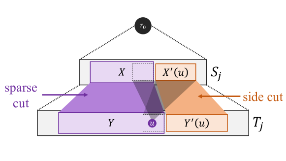
Figure 1: Side cuts and sparse cuts

We note that our new side cuts are much simpler than the sparse cuts from [20]. The interesting thing is that it makes a substantial difference when we take the best of the two. This is proved in the rest of this paper.

5 Analyzing outer round $j$ including side cuts

We are now going to analyze outer round $j$. The novelty relative to [20] is the impact of side cuts together with the small tightening of cut-or-color. Our main result for iteration $j$ will be that

$$|Y_{j}|\leq O(\sqrt{\Psi|T_{j}|}).$$

Since $|T_{j+1}|\leq|Y_{j}|$, this bound can be used recursively.

Cuts.

We claim that any sparse or side cut $(X,Y)$ considered will satisfy

$$\min d_{Y}(X) \geq \Delta_{j}/2$$ (9)

$$|X| \geq \delta_{j}/4$$ (10)

$$|Y| \geq \Delta_{j}^{2}/(8\Psi)$$ (11)

In [20], this was already proved for the sparse cuts $(X,Y)$. More precisely, for sparse cuts, vertices in $X$ preserve all their neighbors in $T_{j}$. This follows recursively from Invariant (iii), and therefore $\min d_{Y}(X)\geq\Delta_{j}$, implying (9). Also (10) follows because $X$ contains the neighborhood of a high $S$-degree vertex, which means degree at least $\delta_{j}/4$. Finally, [20, Eq. (17)] states $|Y|\geq\Delta_{j}^{2}/(2\Psi)$ implying (11).

Lemma 11

Each side cut $(X^{\prime}(u),Y^{\prime}(u))$ satisfies conditions in (9)–(11).

Proof

First, we note that (10) holds because the side cut is only defined if $d_{S_{j}\setminus X}(u)=|X^{\prime}(u)|\geq\delta_{j}/3$.

We now observe that any vertex $v^{\prime}\in S\setminus X$ has at most $\Psi$ neighbors in $Y$ by invariant (iv). Moreover, by (7), $\Delta_{j}={\widetilde{\omega}}(\Psi)$, so the degree from $v^{\prime}\in X^{\prime}(u)$ to $Y^{\prime}(u)$ is at least $\Delta_{j}-\Psi>\Delta_{j}/2$, which implies (9).

For (11), again by (9) the degree from any vertex in $X^{\prime}(u)$ to $Y^{\prime}(u)$ is at least $\Delta_{j}/2$. By Lemma 6, $|Y^{\prime}(u)|\geq\min\{(\Delta_{j}/2)/\Psi,|X^{\prime}(u)|\}\,\Delta_{j}/4$. We have $|X^{\prime}(u)|\geq\delta_{j}/3$ and by pre-condition (8), we have $\delta_{j}\geq 4\Delta_{j}/\Psi$, so $|X^{\prime}(u)|\geq(4\Delta_{j}/3)/\Psi$. Therefore the min evaluates to the first option, so we get $|Y^{\prime}(u)|\geq\frac{\Delta_{j}^{2}}{8\Psi}$, as required in (11).  

Final sparse cut.

In the rest of this section, let $(X,Y)$ denote the last sparse cut considered in outer iteration $j$. The best side cut is then found by calling $\texttt{best-side-cut}(X,Y,S_{j},T_{j})$.

Let $Y^{\prime\prime}\subseteq Y$ be the set of vertices $u\in Y$ such that at least $\delta_{j}/3$ of the $S_{j}$-neighbors of $u$ are in $S_{j}\backslash X$. Then $Y^{\prime\prime}$ are exactly the vertices for which side cuts $(X^{\prime}(u),Y^{\prime}(u))$ are defined.

Lemma 12

We have at least $\delta_{j}|Y|/6$ edges from $Y^{\prime\prime}$ to $S_{j}\backslash X$.

Proof

The loop over sparse cuts in Algorithm 1 only terminates because $|E(S,T)|<\delta_{j}|T|/2$ where $(S,T)$ is our $(X,Y)$. Therefore we must have $|E(Y,S_{j}\setminus X)|\geq\delta_{j}|Y|/2$.

By definition, the vertices from $Y\setminus Y^{\prime\prime}$ have less than $\delta_{j}/3$ edges to $S_{j}\setminus X$ amounting to a total of less than $|Y|\delta_{j}/3$ edges to $S_{j}\setminus X$. Thus we must have at least $\delta_{j}|Y|/2-|Y|\delta_{j}/3=\delta_{j}|Y|/6$ edges from $Y^{\prime\prime}$ to $S_{j}\setminus X$.  

We define

$$\mu=\frac{|Y_{j}|\Psi}{\Delta_{j}^{2}}.$$

Since $Y_{j}$ was a $Y$ from a sparse or side cut $(X,Y)$, (11) implies $\mu\geq 1/8$. We now show the following key lemma, which relates to Lemma 13 in [20] (that is the most important in their analysis).

Lemma 13

The number of edges from $Y^{\prime\prime}$ to $S_{j}\backslash X$ is at most

$$|T_{j}\setminus Y|\,\frac{5\delta_{j}\Psi^{2}}{\mu\Delta_{j}^{2}}.$$ (12)

Proof

We have

$$\sum_{y\in Y}|N_{T_{j}}(N_{S_{j}}(y))\setminus Y| =|\{y\in Y,u\in{T_{j}}\setminus Y\mid N_{S_{j}}(y)\cap N_{S_{j}}(u)\neq\emptyset\}|$$

$$=\sum_{u\in{T_{j}}\setminus Y}|N_{Y}(N_{{S_{j}}}(u))|.$$

Consider any $u\in{T_{j}}\setminus Y$. During the inner loop, there was a first sparse cut $(X^{\prime},Y^{\prime})\supseteq(X,Y)$ with $u\not\in Y^{\prime}$, and then, by Invariant (v), we had $|N_{Y^{\prime}}(N_{N(r_{0})}(u))|<\Psi$. Since $Y^{\prime}\supseteq Y$ and $N(r_{0})\supseteq S_{j}$, this implies $|N_{Y}(N_{S_{j}}(u))|<\Psi$. Thus we have proved

$$\sum_{y\in Y}|N_{T_{j}}(N_{S_{j}}(y))\setminus Y|\leq\,|{T_{j}}\setminus Y|\Psi.$$

We will now relate the above bound to our side cuts $(X^{\prime}(y),Y^{\prime}(y))$ for $y\in Y^{\prime\prime}$. By definition,

$$Y^{\prime}(y)=N_{T_{j}}(N_{S_{j}}(y)\setminus X)\setminus Y\subseteq N_{T_{j}}(N_{S_{j}}(y))\setminus Y.$$

Moreover, $Y^{\prime\prime}\subseteq Y$, so we get

$$\sum_{y\in Y^{\prime\prime}}|Y^{\prime}(y)|\leq|{T_{j}}\setminus Y|\Psi.$$ (13)

Recall that we defined $\mu$ such that

$$\mu\times\frac{\Delta_{j}^{2}}{\Psi}=|Y_{j}|$$

and $|Y_{j}|\leq|Y^{\prime}(y)|$ for all $y\in Y^{\prime\prime}$.

In combination with (13), this implies that

$$|Y^{\prime\prime}|\leq\frac{|{T_{j}}\setminus Y|\Psi}{\mu\times\frac{\Delta_{j}^{2}}{\Psi}}=|{T_{j}}\setminus Y|\frac{\Psi^{2}}{\mu\Delta_{j}^{2}}.$$

We also know that all degrees from $T_{j}$ to $S_{j}$ are bounded by $5\delta_{j}$ and this bounds the size of $X^{\prime}(y)=N_{S_{j}}(y)\setminus X$. We now get the desired bound on the number of edges from $Y^{\prime\prime}$ to ${S_{j}}\backslash X$ as

$$\sum_{y\in Y^{\prime\prime}}|N_{S_{j}}(y)\setminus X| \leq 5\delta_{j}|Y^{\prime\prime}|\leq 5\delta_{j}|T_{j}\setminus Y|\frac{\Psi^{2}}{\mu\Delta_{j}^{2}}=|{T_{j}}\setminus Y|\,\frac{5\delta_{j}\Psi^{2}}{\mu\Delta_{j}^{2}}.$$

 

The number of edges from $Y^{\prime\prime}$ to $S_{j}\backslash X$ are bounded from below by $\delta_{j}|Y|/6$ by Lemma 12 and from above by $|T_{j}\setminus Y|\,\frac{5\delta_{j}\Psi^{2}}{\mu\Delta_{j}^{2}}$ by Lemma 13, so we get

$$|Y|\leq|{T_{j}}|(30\Psi^{2})/(\mu\Delta_{j}^{2}).$$ (14)

Combined with $\mu\times\frac{\Delta_{j}^{2}}{\Psi}=|Y_{j}|\leq|Y|$, we get an upper bound on $\mu$:

$$\mu\leq\frac{\Psi\sqrt{30\Psi|{T_{j}}|}}{\Delta_{j}^{2}}.$$ (15)

We now conclude with the main result from our analysis of our new inner loop:

Lemma 14

$$|Y_{j}|=\mu\times\frac{\Delta_{j}^{2}}{\Psi}\leq\sqrt{30\Psi|T_{j}|}.$$ (16)

Note that if (16) is smaller than the lower bound $\Delta_{j}^{2}/(8\Psi)$ from (11), then progress must have been made before the round finished and this is what are ultimately hoping for.

Comparison to [20].

In [20], there are no side cuts and no $\mu$, so they only had an upper bound corresponding to (14) with $\mu\geq 1/8$, that is,

$$|Y_{j}|\leq O(|{T_{j}}|(\Psi/\Delta_{j})^{2}).$$ (17)

To appreciate the difference, consider the first round where we only have $|T_{1}|\leq n/k$. Then (16) yields $|Y_{1}|=O(n/k^{3/2})$, gaining a factor $\sqrt{k}$ over $n/k$. For comparison, with (17), we gain only a factor $(\Psi/\Delta_{j})^{2}$ which will be subpolynomial by (6).

Proceed to the outer loop

Before going to the outer loop, we give requirements to satisfy during the whole outer loop, which is really the same as that in [20].

We say round $j$ is good if

• the pre-conditions (7) and (8) are satisfied at the beginning of the round.

• No error is made during the round.

• (9)–(11) and (16) are satisfied as long as no progress is made.

Because both our side cuts and the original sparse cuts from [20] satisfy conditions in (9)–(11), a simple generalization of the analysis from [20] implies:

Lemma 15 ([20])

Round $j$ is good if and only if pre-conditions (7) and (8) are satisfied.

The main difference is that our new bound (16) makes it much easier to satisfy the pre-conditions.

6 Analysis of outer loop

Following the pattern in [20], but using our new Lemma 15, we will prove an inductive statement that implies that the outer loop in Algorithm 1 continues with no errors until we make progress with a good coloring. The result, stated below, is both simpler and stronger than that in [20].

Theorem 16

Consider a 3-colorable graph with minimum degree $\Delta\geq\sqrt{n}$. Let

$$k=2^{(\log\log n)^{2}}\sqrt{n/\Delta}.$$ (18)

Algorithm 1 will make only good rounds, and make progress towards an ${\widetilde{O}}\/(k)$ coloring no later than round $\lfloor\log\log n\rfloor$.

Proof

We are going to analyze round $j\leq c=\lfloor\log\log n\rfloor$ of the outer loop. Assuming that all previous rounds have been good, but no progress has been made, we will show that the preconditions of round $j$ are satisfied, hence that round $j$ must also be good. Later we will also show that progress must be made no later than round $j=c$.

To show that the preconditions are satisfied, we will develop bounds for $|T_{j}|$, $\Delta_{j}$, and $\delta_{j}$ assuming that all previous rounds have been good and that no progress has been made. We already know that $|T_{1}|\leq n/k$ and $\Delta_{1}={\widetilde{\Omega}}(\Delta)$. Moreover, $5\delta_{1}\geq\textnormal{avg}\,{d}_{S_{1}}(T_{1})\geq\Delta_{1}|S_{1}|/|T_{1}|\geq\Delta_{1}^{2}k/n$, so $\delta_{1}={\widetilde{\Omega}}(\Delta^{2}k/n)$.

Let us observe that since no progress is made, round $j$ ends up regularizing. As in previous sections, we let $X_{j}$ and $Y_{j}$ denote the last values of $S$ and $T$ in round $j$. Then

$$(S_{j+1},T_{j+1},\Delta_{j+1},\delta_{j+1})=\texttt{regularize}(X_{j},Y_{j}).$$

We will now derive inductive bounds on $|T_{j+1}|$, $\Delta_{j+1}$, and $\delta_{j+1}$.

Computing $\Delta_{j}$.

By Lemma 10 and (9), we get

$$\Delta_{j+1}\geq\textnormal{avg}\,{d}_{Y_{j}}(X_{j})/(30\log n)\geq\Delta_{j}/(60\log n)$$

Inductively, we conclude for any $j$ that

$$\Delta_{j}\geq\Delta_{1}/(60\log n)^{j-1}={\widetilde{\Omega}}(\Delta/(60\log n)^{j}).$$ (19)

We note that $\Delta_{j}$ is just a lower bound on the degrees from $S_{j}$ to $T_{j}$ and we can assume that it is decreasing like in (19).

Satisfying pre-condition (7) stating $\Psi=o(\Delta_{j})$.

By (18) we have

$$\Delta/\Psi=\Delta k^{2}/n=4^{(\log\log n)^{2}}.$$ (20)

For $j<\log\log n$, we have

$$(60\log n)^{j}=\tilde{o}(4^{(\log\log n)^{2}})\textnormal{,}$$

so we get (7) in the stronger from

$$\Psi=\tilde{o}(\Delta_{j}).$$ (21)

Computing $|T_{j}|$.

When we start on the outer loop, we have $|T_{1}|\leq n/k=\Psi k$ and the regularization implies $T_{j+1}\subseteq Y_{j}$, so (16) implies $|T_{j+1}|\leq|Y_{j}|\leq\sqrt{30\Psi|T_{j}|}$. Thus, assuming that nothing goes wrong,

$$|Y_{j}|<30\Psi k^{1/2^{j}}.$$ (22)

Computing $|\delta_{j}|$.

Recall that $\delta_{1}={\widetilde{\Omega}}(\Delta^{2}k/n)$ and consider $j>1$. We have $\textnormal{avg}\,{d}_{X_{j}}(Y_{j})\geq(\Delta_{j}/2)|X_{j}|/|Y_{j}|$ by (9), and $|X_{j}|\geq\delta_{j}/4$ by (10), and $|Y_{j}|<30\,\Psi k^{1/2^{j}}$ by (22). Therefore

$$\textnormal{avg}\,{d}_{X_{j}}(Y_{j})=\Omega\left(\Delta_{j}\delta_{j}/(\Psi k^{1/2^{j}})\right).$$

By Lemma 10

$$\delta_{j+1}={\widetilde{\Omega}}\!\left(\textnormal{avg}\,{d}_{X_{j}}(Y_{j})\right)={\widetilde{\Omega}}\!\left(\Delta_{j}\delta_{j}/(\Psi k^{1/2^{j}})\right)=\delta_{j}\,{\widetilde{\Omega}}\left(\Delta_{j}/\Psi\right)/k^{1/2^{j}}$$

By induction and since the $\Delta_{j}$ are assumed to be decreasing, we get

$$\delta_{j+1}={\widetilde{\Omega}}(\Delta^{2}k/n)\,{\widetilde{\Omega}}\left(\Delta_{j}/\Psi\right)^{j}/k^{1-1/2^{j}}={\widetilde{\Omega}}\left(\Delta_{j}/\Psi\right)^{j}\Delta^{2}k^{1/2^{j}}/n.$$ (23)

Satisfying pre-condition (8) stating $\delta_{j}\geq 4\Delta_{j}/\Psi$.

We note that $\Delta_{j}$ is just a lower bound on the degrees from $S_{j}$ to $T_{j}$ and we can assume that it is decreasing like in (19). The proof is divided into three different cases: $j=1$, $j=2$, and $j>2$. For $j=1$, we have $\delta_{1}={\widetilde{\Omega}}(\Delta^{2}k/n)=(\Delta/\Psi){\widetilde{\Omega}}(\Delta/k)$. Here ${\widetilde{\Omega}}(\Delta/k)=\omega(1)$ by (3), so pre-condition (8) is satisfied.

For larger $j>1$, that is, to make it past the first round, we need lower bounds on the minimum degree $\Delta$. For $j=2$, by (23), $\delta_{2}={\widetilde{\Omega}}\left(\Delta_{1}/\Psi\right)\Delta^{2}k^{1/2}/n$. However, since $\Delta\geq\sqrt{n}$ and $k>\sqrt{n/\Delta}$,

$$\Delta^{2}k^{1/2}/n>\Delta^{2}(n/\Delta)^{1/4}/n\geq n^{1/8}.$$

Thus $\delta_{2}>{\widetilde{\Omega}}\left(\Delta_{1}/\Psi\right)n^{1/8}={\widetilde{\omega}}(\Delta_{1}/\Psi)$. Above we do have some slack in that it would have sufficed with $\Delta>n^{3/7+\Omega(1)}$, but for later rounds, we cannot have $\Delta$ much smaller than $\sqrt{n}$. More precisely, for $j>2$, by (23),

$$\delta_{j+1}={\widetilde{\Omega}}\left(\Delta_{j}/\Psi\right)^{j}\Delta^{2}k^{1/2^{j}}/n\geq{\widetilde{\Omega}}\left(\Delta_{j}/\Psi\right)^{2}\Delta^{2}k^{1/2^{j}}/n={\widetilde{\omega}}(\Delta_{j}/\Psi)\,\Delta^{2}k^{1/2^{j}}/n.$$

The last derivation follows from (21) using $j>2$. With $\Delta\geq\sqrt{n}$, we have $\Delta^{2}k^{1/2^{j}}/n>1$ and (8) follows.

Progress must be made.

Assuming only good rounds, we will now argue that progress must be made no later than round $\log\log n$. Assuming no progress, recall from (22) that

$$|Y_{j}|<30\,\Psi k^{1/2^{j}}.$$

From (11), we know that any $Y$ considered (without progress), including $Y_{j}$, is of size at least $\Delta_{j}^{2}/(8\Psi)$. Thus, if we make it through round $j$ without progress, we must have

$$\Delta_{j}^{2}/(8\Psi)<30\,\Psi k^{1/2^{j}}\iff(\Delta_{j}/\Psi)^{2}<240\,k^{1/2^{j}}$$

By (21), $\Delta_{j}/\Psi={\widetilde{\omega}}(1)$ for $j<\log\log n$, and $k^{1/2^{j}}<2$ for $j=\lceil\log\log k\rceil<\log\log n$, so progress must be made no later than round $j=c=\lfloor\log\log n\rfloor$. This completes our proof of Theorem 16.  

Using Theorem 1, we can show the following:

Theorem 17

In polynomial time, we can color any 3-colorable $n$ vertex graph using ${\widetilde{O}}\/(n^{0.19747})$ colors.

Proof

As in [20], we use Chlamtac’s SDP [7] for low degrees. By Theorem 8, for maximum degree below $\Delta=n^{\tau}$ with $\tau={0.605073}$ and $c=0.0213754$, we can make progress towards $k={\widetilde{O}}\/(n^{0.19747})$ coloring. By Lemma 7, we may therefore assume that $\Delta$ is the minimum degree. This is easily above $\sqrt{n}$, and then by Theorem 16, we get progress towards

$$\sqrt{n/\Delta}2^{(\log\log n)^{2}}=n^{(1-0.605073)/2}2^{(\log\log n)^{2}}<n^{0.19747}.$$

Thus, in polynomial time, we can color any 3-colorable graph with ${\widetilde{O}}\/(n^{0.19747})$ colors.

References

- [1] S. Arora, E. Chlamtac, and M. Charikar. New approximation guarantee for chromatic number. In Proc. 38th STOC, pages 215–224, 2006.
- [2] S. Arora and R. Ge. New tools for graph coloring. In Proc. APPROX-RANDOM, pages 1–12, 2011.
- [3] S. Arora, S. Rao, and U. Vazirani. Expanders, geometric embeddings and graph partitioning. J. ACM, 56(2):1–37, 2009. Announced at STOC’04.
- [4] B. Berger and J. Rompel. A better performance guarantee for approximate graph coloring. Algorithmica, 5(3):459–466, 1990.
- [5] A. Blum. New approximation algorithms for graph coloring. J. ACM, 41(3):470–516, 1994. Combines announcements from STOC’89 and FOCS’90.
- [6] A. Blum and D.R. Karger. An -coloring algorithm for 3-colorable graphs. Inf. Process. Lett., 61(1):49–53, 1997.
- [7] E. Chlamtac. Approximation algorithms using hierarchies of semidefinite programming relaxations. In Proc. 48th FOCS, pages 691–701, 2007.
- [8] I. Dinur, P. Harsha, S. Srinivasan, and G. Varma. Derandomized graph product results using the low degree long code. In Proc. 32nd STACS, pages 275–287, 2015.
- [9] I. Dinur, E. Mossel, and O. Regev. Conditional hardness for approximate coloring. SIAM J. Comput., 39(3):843–873, 2009. Announced at STOC’06.
- [10] U. Feige and J. Kilian. Zero-knowledge and the chromatic number. J. Comput. System Sci., 57:187–199, 1998.
- [11] U. Feige, M. Langberg, and G. Schechtman. Graphs with tiny vector chromatic numbers and huge chromatic numbers. SIAM J. Comput., 33(6):1338–1368, 2004. Announced at FOCS’02.
- [12] M.R. Garey, D.S. Johnson, and L.J. Stockmeyer. Some simplified np-complete graph problems. Theor. Comput. Sci., 1(3):237–267, 1976. Announced at STOC’74.
- [13] M.X. Goemans and D.P. Williamson. Improved approximation algorithms for maximum cut and satisfiability problems using semidefinite programming. J. ACM, 42(6):1115–1145, 1995. Announced at STOC’94.
- [14] V. Guruswami and S. Khanna. On the hardness of 4-coloring a 3-colorable graph. SIAM Journal on Discrete Mathematics, 18(1):30–40, 2004.
- [15] Venkatesan Guruswami and Sai Sandeep. d-to-1 hardness of coloring 3-colorable graphs with O(1) colors. In 47th ICALP, volume 168 of LIPIcs, pages 62:1–62:12, 2020.
- [16] J. Håstad. Clique is hard to approximate within . Acta Math., 182:105–142, 1999.
- [17] D.R. Karger, R. Motwani, and M. Sudan. Approximate graph coloring by semidefinite programming. J. ACM, 45(2):246–265, 1998. Announced at FOCS’94.
- [18] R. M. Karp. On the computational complexity of combinatorial problems. Networks, 5:45–68, 1975.
- [19] K. Kawarabayashi and M. Thorup. Combinatorial coloring of 3-colorable graphs. In Proc. 53rd FOCS, pages 68–75, 2012.
- [20] K. Kawarabayashi and M. Thorup. Coloring 3-colorable graphs with less than n colors. J. ACM, 64(1):4:1–4:23, 2017. Announced at FOCS’12 and STACS’14.
- [21] S. Khanna, N. Linial, and S. Safra. On the hardness of approximating the chromatic number. Combinatorica, 20(3):393–415, 2000.
- [22] M. Szegedy. A note on the number of Lovász and the generalized Delsarte bound. In Proc. 35th FOCS, pages 36–39, 1994.
- [23] A. Wigderson. Improving the performance guarantee for approximate graph coloring. J. ACM, 30(4):729–735, 1983. Announced at STOC’82.