Computation of Maximal Admissible Robust Positive Invariant Sets for Linear Systems with Parametric and Additive Uncertainties
Abstract
In this paper, we address the problem of computing the maximal admissible robust positive invariant (MARPI) set for discrete-time linear time-varying systems with parametric uncertainties and additive disturbances. The system state and input are subjected to hard constraints, and the system parameters and the exogenous disturbance are assumed to belong to known convex polytopes. We provide necessary and sufficient conditions for the existence of the non-empty MARPI set, and explore relevant features of the set that lead to an efficient finite-time converging algorithm with a suitable stopping criterion. The analysis hinges on backward reachable sets defined using recursively computed halfspaces and the minimal RPI set. A numerical example is used to validate the theoretical development.
I Introduction
Admissible and/or invariant sets of dynamical systems can provide valuable insights into their stability and convergence properties, as well as assist in the design of suitable controllers. A set of initial states is said to be positively invariant [1, 2] to a given dynamics if the subsequently evolved states belong to the same set. If this property is achieved despite the presence of uncertainties in the system model, then the set is said to be robust positive invariant (RPI). In most practical applications, the system state, input, output or their combination is subjected to constraints, thus motivating the development of maximal constraint admissible sets [3], the largest possible set of initial states that evolve following the given dynamics while satisfying the imposed constraints.
Existing literature has extensively dealt with RPI and maximal admissible sets for both linear and nonlinear systems, primarily in discrete-time setting. Some interesting applications include controller design for humanoid robots and systems in specialized Lie groups, design of control barrier functions, guaranteeing feasibility in model predictive control (MPC), etc., (see [4, 5, 6, 7, 8, 9]). One of the earliest theoretical works [3] details various properties of a maximal output admissible (MOA) set for an autonomous linear time-invariant (LTI) system along with an algorithm for computing the same. A known non-autonomous system is considered in [3] that transforms to an autonomous system on application of state feedback control. The concept in [3] is extended to MOA sets for discrete-time LTI systems with bounded exogenous disturbance in [10], and to linear time-varying (LTV) systems with polytopic uncertainty in the parameters in [11]. The procedure for construction of MOA sets for nonlinear systems with exact model knowledge is provided in [12, 13, 14], and that for bilinear systems in [15]. The works in [16] and [17] focus on MOA sets that satisfy output constraints with certain probability for time-invariant and time-varying parametric uncertainties, respectively. A few works [18, 19, 20, 21, 22] describe constraint admissible RPI sets for linear systems with both parametric and additive uncertainties.
In this paper, we deal with the maximal admissible RPI (MARPI) set for LTV systems with polytopic parametric uncertainties and polytopic additive disturbances. The LTV system is transformed to an autonomous system using state feedback control with a quadratically stabilizing feedback gain [23, 24]. The system state and input are subjected to polytopic hard constraints. Unlike the sets introduced and constructed in [3, 4, 5, 6, 7, 8, 9, 10, 11, 17, 16, 15, 12, 13, 14] that are positively invariant to known dynamics, or RPI to either parametric uncertainty or external disturbances, the proposed MARPI set is invariant to both parametric and additive uncertainties. This work, inspired from [10] and [11], seeks to rigorously analyse properties of the MARPI set that are required to design and implement a tractable algorithm. Theoretically, the computation of an MARPI set involves infinite intersections of -step backward reachable sets where varies from zero to infinity [10, 11]. The proposed algorithm is similar in spirit to the standard method of constructing MOA sets in [3, 10, 11]. However, the main challenges that this work addresses include construction of the backward reachable sets, necessary and sufficient conditions for the MARPI set to be non-empty, showing that the set is obtainable with finite intersections, and proving that a stopping criterion exists for the algorithm.
Due to the presence of both parametric and additive uncertainties, it is required to consider all possible combinations of additive disturbance for every possible value of the uncertain parameters in defining the halfspaces that form the backward reachable sets. Carrying out theoretical analysis using such set definitions becomes cumbersome. This is overcome by strategically defining the halfspaces in a recursive fashion using the vertices of the parametric uncertainty set, support functions of the disturbance set and Kronecker product. Different from [11], the additional challenge in this work is that of non-existence of the MARPI set due to the presence of disturbance. It is, therefore, prudent to check the existence of the MARPI set before attempting to compute it using the algorithm. We state necessary and sufficient conditions to check the existence of the non-empty MARPI set. A similar situation arises in [10] that considers additive disturbance only, where the minimal RPI (mRPI) set is used to obtain the existence condition. Owing to the absence of parametric uncertainty, the mRPI set in [10] is convex. For the case in question, where both parametric and additive uncertainties are considered, the mRPI set is a union of infinite convex sets, and the union may be non-convex. Consequently, the results in [10, 11] do not trivially extend to the case of parametric and additive uncertainties. Constraint admissible RPI sets for systems with both types of uncertainties have also been addressed in [18, 19, 20, 21, 22]. An inclusion-based mRPI set is constructed in [18] whereas [19, 20, 21, 22] deal with MARPI sets. In [19], the theory and computation of maximal -contractive set (with ) is discussed and used to design a suitable feedback control. For linear systems, the designed feedback gain in [19] depends on set-induced Lyapunov function, and is therefore, not fixed for all points in the contractive set. Contrary to this, we construct the MARPI set for a given quadratically stabilizing feedback gain without considering the restrictive property of contraction. In [20], a Schur stable nominal system along with small admissible perturbations as feedback that consist of stable, time-varying, memoryless and possibly nonlinear operators is considered. The parametric uncertainty is modeled using the operator assumed to be norm-bounded by one. Chapter 3 in [21] lays down the theory of computing MARPI sets without providing a detailed algorithm or other associated conditions for obtaining the set. In [22], a robust command governor is designed based on the computation of the MARPI set.
In this paper, we focus on polytopic parametric and additive uncertainties, and show in detail that the existence condition of the non-empty MARPI set can be obtained using the computable convex hull of the mRPI set [18]. Provided the MARPI set is non-empty, we prove that it can be obtained with finite intersections of the suitably defined backward reachable sets. Thereafter, we show the existence of a stopping criterion leading to a tractable algorithm.
Notations and Definitions: and represent and -norms of a vector (or induced and -norms of a matrix), respectively. is the empty set. The Minkowski sum of two sets and is denoted by . The set operations and where is a matrix. is the zero vector, is a vector in with each element equal to , and denotes Kronecker product. with integers and . The convex hull of the set of elements is denoted by . For any , returns the greatest integer less than or equal to . The symbol denotes the row of a matrix/vector . For two vectors , or implies . The support function of the set evaluated at the vector is represented by where ‘’ denotes supremum. The function maps the matrix to a vector of the support functions of evaluated at the transpose of each row of , i.e.,
| (1) |
where are the consecutive rows in .
II Problem Formulation
Consider the following discrete-time LTV system
| (2) | |||
| (3) |
where is the state, is the input, , are system parameters, is an additive disturbance and (3) are hard constraints on the system state and input. We define an augmented parameter . The parameter and the additive disturbance are unknown but belong to the sets and , respectively. For all the elements in of the form where and , there exists a common gain such that is Schur stable. In other words, any system , where , is quadratically stabilizable using the feedback gain [23, 24]. The sets , , and are known convex polytopes, each containing its respective origin.
The objective is to find the MARPI set that satisfies where . The input transforms the non-autonomous system in (2) to an autonomous system with exogenous disturbance. Here, ‘admissible’ refers to the satisfaction of (3) whereas ‘robustness’ is with respect to the uncertain parameters , , and the external disturbance .
III Reformulation of the objective
The polytopes and can be represented using their halfspaces, and using its vertices as follows:
| (4) | |||
| (5) | |||
| (6) | |||
| (7) |
where the vertex , is finite, and and are known. Using the feedback gain , two more polytopic sets are defined below:
| (8) | |||
| (9) | |||
where each element in is Schur stable since is a quadratically stabilizing feedback gain. By definition (8), the elements of satisfy (3), i.e., and . Therefore, our objective can be modified to finding the MARPI set , where , for the dynamics
| (10) |
i.e., following (LABEL:invdyn). Redefining the objective in the above manner circumvents the harder task of finding the MARPI set in for which .
IV Construction of the MARPI Set
Consider a set . The right-hand side of the inequality involves subtraction , from which it can be deduced that the irredundant halfspaces contributing to the set definition are the ones that correspond to the worst case disturbance. To reduce computation, instead of subtracting with all , it is preferable to use the function , defined in (1), which is a vector of support functions (see Notations and Definitions) that capture the worst effect of the disturbance, and then redefine . By definition, is the set of all states that enter in one time step following the dynamics in (LABEL:invdyn). Similarly, we can define sets
| (11) |
where is the set of all states that enter in time steps.
Theorem 1
Proof:
By definition of in (11), if the initial state , then, following the dynamics in (LABEL:invdyn), the state . Therefore, the intersection of the sets yields the set of all possible states such that following the dynamics in (LABEL:invdyn). Further, for any , we can write
where and , i.e., . Therefore, is an admissible RPI set.
If , then is the maximal. If , consider any element . Then, at least one such that if , the state will leave . This implies that any does not belong to an admissible RPI set, and therefore, is the MARPI set.
Since the dynamics in (LABEL:invdyn) is linear, each of the sets can be represented as the intersection of halfspaces as defined in (11). Consequently, the set is obtained by the intersection of infinite halfspaces. Let . Then, and where the pair represents any of the halfspaces forming . For any , . This is true for all the halfspaces of , which proves that is convex. ∎
Computing the sets as defined in (11) is intractable since there are infinite halfspaces owing to infinite number of elements . The following lemma shows that it is in fact sufficient to construct using only the vertices of instead of each individual element in .
Lemma 1
Proof:
See subsection A in the Appendix. ∎
Although Lemma 1 enables recursive computation of the sets , it is still practically impossible to perform the infinite intersections in (12) for obtaining . However, (12)-(15) are useful for gaining insight into some properties of , based on which a tractable algorithm is mentioned in Section V.
The subtraction of the support functions in the computation of each may result in being empty; therefore, we propose conditions to check the existence of the non-empty MARPI set . To this end, consider
| (16) |
In the limiting case when in (16), we obtain which is the union of infinite convex sets, and is called the mRPI set111With and the bounded uncertainties and , all possible values of and further, .[18, 25]. The union may be non-convex, and computing such a set is challenging. For deriving the existence condition of a non-empty , we show that it suffices to use the convex hull of given by , where
| (17) |
The set can be constructed following the algorithm developed in [18] using the recursion in (17). In the next theorem, we establish the necessary and sufficient conditions for the existence of the non-empty MARPI set.
Theorem 2
For the system given in (LABEL:invdyn),
(a) the MARPI set exists iff the mRPI set .
(b) Alternatively, let where . The set exists iff .
Proof:
(a) By definition, the MARPI set is required to be a subset of . If the minimal RPI set , then there can not exist any other non-empty admissible RPI set in . This implies exists only if .
Further, if , then at least one admissible RPI set , guaranteeing the existence of . In other words, guarantees that each row entry in resulting in non-empty , and since each contains the origin, the set is non-empty and therefore, exists.
(b) Let each of the infinite convex sets whose union forms be denoted by where . From (a), exists
iff (since is convex) ∎
Next, we show that if exists, then it can be obtained with finite intersections, unlike (12). To achieve this, define
| (18) |
Lemma 2
If , then
Proof:
See subsection B in the Appendix. ∎
Theorem 3
If the conditions for the existence of given in Theorem 2 hold, then a finite integer such that , i.e., can be finitely determined.
Proof:
We show that a finite integer for which , which is sufficient to prove the theorem statement. Let . For some integer , we can write
| (19) |
The largest element in is which is upper bounded by . Also, note that by definition, , where . If for some , then , implying . To investigate if a finite satisfying , consider the two cases given below.
(a) When , which is finite since is finite and is a polytope. Let . From Lemma 2, we know that . Therefore, a finite such that , and . Note that owing to the finite number of intersections, the set is a polytope.
(b) When , due to which . However, since is quadratically stabilizing, a Lyapunov function for the dynamics . Let represent a transformed setup obtained using , i.e., the transformed state and sets , and resulting in . Now, similar to the proof in (a), a finite and a set , the MARPI set in the transformed setup. Since can be finitely determined, a finite in the original setup such that the set can also be finitely determined. ∎
Using Theorem 3, an implementable approach for computing would be to perform the intersections by finding the sets . The brute-force method to carry this out is to obtain and with the intersection given by . However, even with a finite , the number of rows in and grow exponentially with (see (14), (15)), resulting in high computational burden.
Also, note that a finite is used in Theorem 3 for the sake of proving that is obtainable with finite intersections. It may be possible to obtain the set with less than number of intersections since the proof of Theorem 3 is performed using a conservative upper bound of the elements of and a conservative lower bound of the elements of . Instead of using and , motivated by [11], we propose a more elegant and less computationally burdensome algorithm for computing the set .
V Tractable method to compute the MARPI Set
In this section, we present a tractable algorithm for computing the MARPI set without knowing the value of . We begin by developing a stopping criterion for performing the finite set intersections.
Theorem 4
Suppose the conditions for the existence of given in Theorem 2 are satisfied. Let , where . The set iff .
Proof:
Using the definitions of in (11) and , we know that implies all elements of enter after one time step evolution following the dynamics in (LABEL:invdyn), i.e., . Also, (by definition of ). Similarly, . To summarize, .
Now, following the same analysis, if , then implying . Using , we can write ,
| (20) | |||
| (21) |
implying since in steps the elements of enter (see (20) and (21)). Therefore, implies (since ).
Also, , which completes the proof. ∎
To compute , initialize a set . Define the precursor set of as . Clearly, . At iteration 1, update . The updated is the maximal set of all states in that stay in after one time step evolution following (LABEL:invdyn). Now, . Updating in the iteration as gives the maximal set of all states in that stay in after one as well as two time steps evolution. For the newly obtained set , we have, .
In general, the where is obtained at iteration . The recursive process of reassigning is continued until . The set obtained when the condition is satisfied yields the MARPI set as proved in the following corollary.
Corollary 1
If , then .
Proof:
Denote the set obtained at iteration by . By construction, . If , then
. Therefore, and . This is similar to the statement of Theorem 4, thus, yielding , the MARPI set. ∎
The steps to implement this process of updating are given in Algorithm 1. This technique also involves repeated intersections. However, it uses the operation that computes only the one-step backward reachable set at each iterative step, thus, reducing the amount of computation. In fact, the computational burden can be further reduced by running a simple linear programming (LP) problem (see (22) in Algorithm 1) that takes into account only the irredundant halfspaces of the intersection at each iteration.
Remark 1
Remark 2
Instead of (or in addition to) the state and input constraints in (3), it is possible to have output constraints. Let the output be , where , and with known and . If the invariant set has to satisfy only the output constraint , then Algorithm 1 can be used with and , and the resulting set is the MOARPI set. In presence of both output and input constraints, and .
Remark 3
In MPC, the terminal set is typically used to establish recursive feasibility and stability [8, 26, 27]. To reduce the prediction horizon length and consequently, the computational burden in robust MPC, it is desired that the set is MARPI. An algorithm for generating such a terminal set is mentioned in [26, Appendix A.1] for systems with both additive and parametric uncertainties. However, the algorithm depends on the choice of a basic polytope ( in [26]) for robust tubes [28] and may result in a subset of the actual MARPI set. A better approach may be to first find the MARPI set, and then use it as the terminal set as well as the basic polytope for generating the tubes.
Remark 4
The proposed theory is trivially extendable for a time-varying that is common for all elements in at time (or a parameter-dependent ), where is a known polytope, provided the resulting set and , is a convex polytope with each element being Schur stable and .
VI Simulation Result
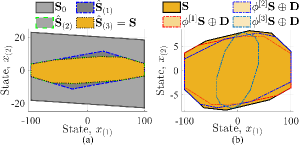
Consider the order LTV system: with , , , , and 222, and .
Figure 1 is obtained with a quadratically stabilizing feedback gain . The sets at each iterative step converging to the set are shown in Fig. 1(a). The algorithm converges in iterations and the set can be represented using only irredundant halfspaces. In Fig. 1(b), we see that which verifies the robust positive invariance property of .
VII Conclusion
The paper extends the results of [10, 11] to MARPI set for state and input constrained discrete-time LTV systems having both polytopic parametric and additive uncertainties. A verifiable necessary and sufficient condition for the existence of the non-empty MARPI set is obtained using the convex hull of the mRPI set. The MARPI set, if exists, is shown to be computable in finite time using a suitable stopping criterion leading to a tractable algorithm with possible applications in robust MPC, safe controller design using control barrier functions, etc. Future work will consider finding MARPI sets for systems with nonconvex polyhedral constraints [29], and also enlarging the domain of attraction for MPC by computing precursor sets which need not be invariant [30].
Appendix
VII-A Proof of Lemma 1
Let . Since is defined , we have . Next, assume . Then, a that satisfies . However, each can be represented as the convex hull of the vertices of , i.e., for such that and . This allows us to write . This contradicts our assumption. Therefore, implying . Continuing similarly, it can be shown that , which concludes the proof.
The definition of in (14) is easy to follow. For comprehending in (15), we explain the construction of and . In , we have that needs be repeated times for vertices, and so, . For , we need corresponding to each . Considering the vertex-based definition, we require times repetition of , and times repetition of to obtain . Following similar steps yields definition (15) of .
VII-B Proof of Lemma 2
References
- [1] F. Blanchini, “Set invariance in control,” Automatica, vol. 35, no. 11, pp. 1747–1767, 1999.
- [2] F. Blanchini, S. Miani, et al., Set-theoretic methods in control. Springer, 2008, vol. 78.
- [3] E. Gilbert and K. Tan, “Linear systems with state and control constraints: the theory and application of maximal output admissible sets,” IEEE Trans. Automat. Contr., vol. 36, no. 9, pp. 1008–1020, 1991.
- [4] K. Yamamoto and T. Shitaka, “Maximal output admissible set for limit cycle controller of humanoid robot,” in IEEE Int. Conf. Robot. and Automat. (ICRA), 2015, pp. 5690–5697.
- [5] A. Weiss, F. Leve, M. Baldwin, J. R. Forbes, and I. Kolmanovsky, “Spacecraft constrained attitude control using positively invariant constraint admissible sets on ,” in Amer. Contr. Conf., 2014, pp. 4955–4960.
- [6] V. Freire and M. M. Nicotra, “Systematic design of discrete-time control barrier functions using maximal output admissible sets,” IEEE Contr. Syst. Lett., vol. 7, pp. 1891–1896, 2023.
- [7] C. Danielson and T. Brandt, “Constraint admissible positive invariant sets for vehicles in SE(3),” IEEE Contr. Syst. Lett., vol. 7, pp. 3759–3764, 2023.
- [8] E. Kerrigan and J. Maciejowski, “Invariant sets for constrained nonlinear discrete-time systems with application to feasibility in model predictive control,” in IEEE Conf. Decis. and Contr., vol. 5, 2000, pp. 4951–4956.
- [9] B. Pluymers, J. Rossiter, J. Suykens, and B. De Moor, “Interpolation based MPC for LPV systems using polyhedral invariant sets,” in Amer. Contr. Conf., 2005, pp. 810–815.
- [10] I. Kolmanovsky and E. G. Gilbert, “Maximal output admissible sets for discrete-time systems with disturbance inputs,” in Amer. Contr. Conf., vol. 3, 1995, pp. 1995–1999.
- [11] B. Pluymers, J. A. Rossiter, J. A. Suykens, and B. De Moor, “The efficient computation of polyhedral invariant sets for linear systems with polytopic uncertainty,” in Amer. Contr. Conf., 2005, pp. 804–809.
- [12] K. Hirata and Y. Ohta, “Exact determinations of the maximal output admissible set for a class of nonlinear systems,” Automatica, vol. 44, no. 2, pp. 526–533, 2008.
- [13] J. M. Bravo, D. Limón, T. Alamo, and E. F. Camacho, “On the computation of invariant sets for constrained nonlinear systems: An interval arithmetic approach,” Automatica, vol. 41, no. 9, pp. 1583–1589, 2005.
- [14] M. Rachik, M. Lhous, and A. Tridane, “On the maximal output admissible set for a class of nonlinear discrete systems,” Syst. Anal. Modelling Simul., vol. 42, no. 11, pp. 1639–1658, 2002.
- [15] Y. Benfatah, A. El Bhih, M. Rachik, and A. Tridane, “On the maximal output admissible set for a class of bilinear discrete-time systems,” Int. J. Contr., Automat. and Syst., vol. 19, pp. 3551–3568, 2021.
- [16] T. Hatanaka and K. Takaba, “Probabilistic output admissible set for systems with time-varying uncertainties,” Syst. & Contr. Lett., vol. 57, no. 4, pp. 315–321, 2008.
- [17] T. Hatanaka and K. Takaba, “Computations of probabilistic output admissible set for uncertain constrained systems,” Automatica, vol. 44, no. 2, pp. 479–487, 2008.
- [18] K. I. Kouramas, S. V. Rakovic, E. C. Kerrigan, J. C. Allwright, and D. Q. Mayne, “On the minimal robust positively invariant set for linear difference inclusions,” in IEEE Conf. Decis. and Contr., 2005, pp. 2296–2301.
- [19] F. Blanchini, “Ultimate boundedness control for uncertain discrete-time systems via set-induced lyapunov functions,” IEEE Trans. Automat. Contr., vol. 39, no. 2, pp. 428–433, 1994.
- [20] K. Hirata and Y. Ohta, “The maximal output admissible set for a class of uncertain systems,” in IEEE Conf. Decis. and Contr., vol. 3, 2004, pp. 2686–2691.
- [21] E. C. Kerrigan, “Robust constraint satisfaction: Invariant sets and predictive control,” Ph.D. dissertation, University of Cambridge UK, 2001.
- [22] A. Casavola, E. Mosca, and D. Angeli, “Robust command governors for constrained linear systems,” IEEE Trans. Automat. Contr., vol. 45, no. 11, pp. 2071–2077, 2000.
- [23] P. P. Khargonekar, I. R. Petersen, and K. Zhou, “Robust stabilization of uncertain linear systems: quadratic stabilizability and control theory,” IEEE Trans. Automat. Contr., vol. 35, no. 3, pp. 356–361, 1990.
- [24] M. C. De Oliveira, J. Bernussou, and J. C. Geromel, “A new discrete-time robust stability condition,” Syst. & Contr. Lett., vol. 37, no. 4, pp. 261–265, 1999.
- [25] S. V. Rakovic, E. C. Kerrigan, K. I. Kouramas, and D. Q. Mayne, “Invariant approximations of the minimal robust positively invariant set,” IEEE Trans. Automat. Contr., vol. 50, no. 3, pp. 406–410, 2005.
- [26] M. Lorenzen, M. Cannon, and F. Allgöwer, “Robust MPC with recursive model update,” Automatica, vol. 103, pp. 461–471, 2019.
- [27] A. Dey, A. Dhar, and S. Bhasin, “Adaptive output feedback model predictive control,” IEEE Contr. Syst. Lett., vol. 7, pp. 1129–1134, 2023.
- [28] W. Langson, I. Chryssochoos, S. Raković, and D. Q. Mayne, “Robust model predictive control using tubes,” Automatica, vol. 40, no. 1, pp. 125–133, 2004.
- [29] E. Pérez, C. Arino, F. X. Blasco, and M. A. Martínez, “Maximal closed loop admissible set for linear systems with non-convex polyhedral constraints,” J. of Process Contr., vol. 21, no. 4, pp. 529–537, 2011.
- [30] D. Limon, T. Alamo, and E. F. Camacho, “Enlarging the domain of attraction of MPC controllers,” Automatica, vol. 41, no. 4, pp. 629–635, 2005.