E³-Net: Efficient E(3)-Equivariant Normal Estimation Network

Abstract

Point cloud normal estimation is a fundamental task in 3D geometry processing. While recent learning-based methods achieve notable advancements in normal prediction, they often overlook the critical aspect of equivariance. This results in inefficient learning of symmetric patterns. To address this issue, we propose E³-Net to achieve equivariance for normal estimation. We introduce an efficient random frame method, which significantly reduces the training resources required for this task to just 1/8 of previous work and improves the accuracy. Further, we design a Gaussian-weighted loss function and a receptive-aware inference strategy that effectively utilizes the local properties of point clouds. Our method achieves superior results on both synthetic and real-world datasets, and outperforms current state-of-the-art techniques by a substantial margin. We improve RMSE by 4% on the PCPNet dataset, 2.67% on the SceneNN dataset, and 2.44% on the FamousShape dataset.

1 Introduction

Normal estimation for point cloud analysis is a fundamental and essential task in 3D vision. It involves accurately determining the surface normals for each point and thus plays a crucial role in numerous applications, e.g., 3D reconstruction [1, 2], object recognition [3, 4], denoising [5, 6], …

Traditional methods for normal estimation include, Principal Component Analysis (PCA) [7], n-jet [8], Moving Least Squares (MLS) [9, 10], Voronoi-based method [11], Hough transform [12] and winding-number field [13]. While these classical methods have laid the groundwork for point cloud processing, their limitations in handling noise, computational efficiency, adaptability to complex structures, and dependency on data density necessitate further advancements in the field.

Recent neural network-based algorithms for estimating normals in point clouds can overcome many of the challenges of traditional methods. PCPNet [14] proposed a single-patch-based framework, which was followed by n-jet fitting methods [15, 16, 17] and implicit surface methods [18, 19]. Recently, MSECNet [20] introduced a patch-to-patch approach, further improving efficiency and accuracy. Additionally, compared with traditional approaches like PCA and MLS, learning-based methods lack invariant properties that are independent of the point cloud’s embedding in three-dimensional (3D) space, particularly those relying on GNN [21] or PointNet [22] architectures. As a result, their results may vary with changes in orientation or position, as these methods do not inherently guarantee such properties. Equivariant networks like frame averaging [23] and E($n$)-GNN [24] can mitigate this issue but often require significantly increased inference time or parameter count for training.

To address the aforementioned issues, building on the analysis of E(3)-equivariance presented in Puny et al. [23], we develop a novel method termed E³-Net, an Efficient E(3)-Equivariant network for normal estimation that enables both equivariance and efficiency. Instead of employing a large network that processes multiple frames jointly, we utilize a smaller, more efficient network that processes one frame at a time. This approach requires only 1/8 of the training resources.

Furthermore, we tackle inefficiencies due to the number of patches being processed. Processing a single patch for each point, may have higher accuracy, but is highly inefficient. In contrast, predicting normals for all points within a patch significantly increases efficiency but introduces issues at boundaries, as boundary points have a smaller receptive field. To address these challenges, we develop a new loss function that incorporates Gaussian weighting, which enables simultaneous prediction of normals for all points in an entire patch.

To increase the receptive field during the testing phase, we introduce a novel receptive-aware inference strategy that supplants the traditional k-nearest neighbor method with geodesic patch sampling. Additionally, we refine our aggregation strategy to be receptive-aware, drawing inspiration from mean filtering and Gaussian filtering, as reviewed by Buades et al. [25]. This method effectively harnesses information from overlapping patches, thus significantly improving the performance of our model.

We conduct extensive comparative experiments to demonstrate the efficacy of the proposed method on typical benchmark datasets, including PCPNet [14], FamousShape [19], and real-world SceneNN [18]. Our method consistently outperforms current state-of-the-art models. Furthermore, we validate the practical application potential of our algorithm by utilizing the predicted normals for 3D Poission reconstruction [1]. To summarize, the main contributions of this work are as follows:

• a novel method for random frame training which ensures both efficiency and equivariance in the network (See Sec. 4.1).

• a novel Gaussian-weighted loss function, for efficient patch-based processing without loss of accuracy (See Sec. 4.2).

• a receptive-aware inference strategy using geodesic patches and weighted aggregation (See Sec. 4.3).

2 Related Work

We present an overview of traditional normal estimation, learning-based normal estimation, and E($n$)-equivariant networks.

Traditional Normal Estimation. In point cloud normal estimation, traditional methods typically involve analyzing a small neighborhood around each point. PCA [7] examined local covariance within a small area to determine the direction of minimal variance as the normal. MLS [9] fits a plane to local points for normal estimation. n-Jets [8] estimated normals by fitting higher-order polynomial surfaces to point cloud data, while Merigot et al. [11] leveraged the covariance matrices of Voronoi cells to predict normals. The Hough Transform method [12] interpreted the filled accumulator as a discrete probability distribution, where the most probable normal direction was determined by the maximum value in this distribution. These traditional methods are generally sensitive to noisy data and do not perform as well as learning-based alternatives.

Learning-based Normal Estimation. Early work, PCPNet [14] proposed a patch-based normal prediction framework. Zhou et al. [26] employed local plane constraints and multi-scale selection in their approach. MTRNet [27] focused on learning latent tangent spaces combined with a compact multi-scale approach. Furthermore, Nesti-Net [28] integrated multi-scale analysis with 3D convolutional neural networks. Lessen et al. [29] proposed a method involving iterative surface fitting, neural network-driven inference, and adaptive kernel refinement. In addition, Refine-Net [30] integrated advanced feature representations with a novel connection module within a geometrically-focused framework. Zhang et al. [31] introduced a geometry-weighted guidance approach, combined with multi-scale normal integration and error correction networks. In jet-based approaches, DeepFit [15] combined PointNet-based weight prediction with jet fitting to enhance the robustness and data efficiency in normal estimation. AdaFit [16] introduced an offset prediction mechanism in jet fitting to adaptively handle complex surface geometries, while Graphfit [17] combined graph-convolutional learning, adaptive attention-based fusion, and multi-scale representation to further enhance normal estimation accuracy. Du et al. [32] focused on $z$-direction transformation and normal error estimation, which can be flexibly integrated with current polynomial surface fitting methods for point cloud normal estimation. Additionally, NeAF [33] innovatively learned an angle field around point normals, predicting offsets between input vectors and true normals. HSurf-Net [18] combined hyper surface fitting in a high-dimensional feature space without the need for adjusting the order. Recent developments like SHS-Net [19] and NGL [34] focused on oriented point normal estimation, typically using a one-patch-per-point prediction approach, which is less efficient. More recently, MSECNet [20] adopted a patch-to-patch prediction method, enhancing efficiency over other methods. Different from previous approaches, our work features all three important attributes: equivariance, efficiency, and accuracy (beating all previous methods).

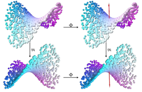
Figure 1: An illustration of the E(3)-equivariance, where $\Phi$ is an E(3)-equivariant function predicting a point’s normal, and $g$ is an element of the E(3) group. These two operators are commutative, meaning that the order in which they are applied does not affect the final outcome.

E($n$)-Equivariant Networks Significant advancements have been achieved in neural networks regarding symmetry invariance and equivariance [35, 36, 37, 38, 39], expanding applications across various fields. SchNet [40] exemplified this progress by modeling quantum interactions with rotationally invariant energies and equivariant forces. Tensor field networks [41] introduced rotation, translation, and permutation equivariance at each layer, enhancing feature identification. Equivariant flows [42] innovated in symmetric energy sampling for multi-body systems, guiding the design of symmetry invariant Boltzmann generators. E($n$)-equivariant graph neural networks [24] demonstrated its equivariance to rotations, translations, reflections, and permutations, without relying on higher-order representations. Additionally, SE(3)-transformers [43] marked a leap with their 3D roto-translationally equivariant self-attention module. Frame averaging [23] emerged as a highly efficient and robust approach, adapting neural architectures to various symmetries, which led to applications in equivariant shape space learning [44]. E3Sym [45] showcased E(3) invariance in unsupervised 3D planar reflective symmetry detection. FAENet [46] highlighted the use of frame averaging equivariant GNN in materials modeling, proving the effectiveness of E(3)-equivariant GNNs.

3 Preliminaries

Definition 1.

The Euclidean group E($n$) that encompasses all isometric transformations including rotations, reflections, and translations within $n$ dimension is defined as:

$${\mathrm{E}(n)}={\mathrm{O}(n)}\ltimes\mathbb{R}^{n}\triangleq\{(\mathbf{R},\mathbf{v})\mid\mathbf{R}\in\mathrm{O}(n),\mathbf{v}\in\mathbb{R}^{n}\},$$ (1)

where $\ltimes$ is the semidirect product operator and O($n$) signifies the set of $n\times n$ orthogonal matrices expressed as:

$${\mathrm{O}(n)}=\{\mathbf{R}\in\mathbb{R}^{n\times n}\mid\mathbf{R}\mathbf{R}^{T}=\mathbf{R}^{T}\mathbf{R}=\mathbf{I},\det(\mathbf{R})=\pm 1\}.$$ (2)

Definition 2.

A function $\Phi$ is considered to be E($n$)-equivariant if, when an input $\mathbf{x}$ is transformed by an element $g\in\mathrm{E}(n)$, the resulting output of the function is likewise transformed by $g$. Formally, this is expressed as:

$$\Phi(g(\mathbf{x}))=g(\Phi(\mathbf{x})),\ \text{for all}\ g\in{\mathrm{E}(n)}.$$ (3)

This concept plays a crucial role in normal estimation. As shown in Fig. 1, equivariance ensures that estimating normals using a local patch and then applying an isometric transformation to the estimated normals is equivalent to first applying an isometric transformation to the local patch and then estimating the normals. The outcome remains consistent regardless of the order in which isometric transformation and normal estimation are applied.

Frame Construction. Given an input point patch $\mathbf{x}\in\mathbb{R}^{m\times 3}$, we first calculate its centroid denoted as $\boldsymbol{t}$, and then we compute its covariance matrix. Assume that the eigenvalues of this covariance matrix are ordered in ascending order, e.g., $\lambda_{1}\leq\lambda_{2}\leq\lambda_{3}$. Corresponding to these eigenvalues, we have normalized eigenvectors denoted by $\boldsymbol{v}_{1},\boldsymbol{v}_{2},\boldsymbol{v}_{3}$. Then, the frame set that relates $\boldsymbol{v}_{i}$ and $\boldsymbol{t}$ belonging to $\mathrm{E}(3)$ is constructed as [23]

$$\mathcal{F}(\mathbf{x})=\left\{\left([\pm\boldsymbol{v}_{1},\pm\boldsymbol{v}_{2},\pm\boldsymbol{v}_{3}],\boldsymbol{t}\right)\right\}\subset\mathrm{E}(3).$$ (4)

Note that the frame set has $2^{3}$ elements. Compared to the uncountable E(3), the frame set constructed in Eq. 4 contains only a finite number of elements (8), yet it includes all the information necessary for the algorithm to possess E(3)-equivariance, which offers a systematic approach for algorithm design.

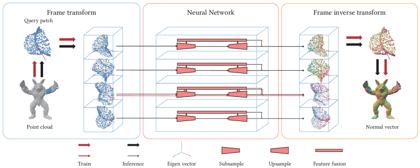
Figure 2: Illustration of the proposed framework. The red arrows depict the training process, while the black arrows represent the inference phase. The diagram only shows 4 elements in the frame set.

4 Methodology

In this section, we present our main contributions: efficient E(3)-equivariance (Sec. 4.1), a Gaussian weighted loss function (Sec. 4.2), and receptive-aware inference (Sec. 4.3).

4.1 Efficient E(3)-Equivariance

To ensure the E(3)-equivariant property, we adopt the frame averaging method defined by the following equation,

$$\Phi(\mathbf{x})=\frac{1}{|\mathcal{F}(\mathbf{x})|}\sum_{g\in\mathcal{F}(\mathbf{x})}g\phi(g^{-1}\mathbf{x}),$$ (5)

This approach utilizes $\mathcal{F}(\mathbf{x})$, a small subset of the group for averaging, thus making the process more practical for applications involving the Euclidean group E(3). In our context, $\Phi$ represents the E(3)-equivariant normal estimation network.

Although Eq. 5 guarantees E(3)-equivariance (theoretical proof is presented in the Appendix A), the training of a network that involves all frames simultaneously, typically requires substantial computational resources and is difficult to optimize. To boost the efficiency, we further propose a random frame strategy as illustrated in Fig. 2. During the training stage, a random frame ${\mathcal{F}(\mathbf{x})}_{i}$ is first chosen from ${\mathcal{F}(\mathbf{x})}$. Then the data is transformed to this frame before being fed into the network. Our random scheme not only assures E(3)-equivariance, but also allows $\phi$ to handle data in various frames more efficiently. During inference, this transformation can be directly applied to implement $\Phi$, facilitating the processing of data in its original frame context, thereby achieving E(3)-equivariant property without the need of training the entire $\Phi$. In summary, previous work [23] focused on $\Phi$ on the left side of the equation computing all eight frames jointly, but we focus $\phi$ on the right side computing one $\phi$ at a time. This leads to a factor 8 improvement in efficiency considering the size of the network, while at the same time improving accuracy.

4.2 Loss Function

In our method, two loss functions are utilized to estimate normals. The first function is defined as a regression loss, which minimizes the Euclidean distance between the predicted normals and the ground truth:

$$\mathcal{L}^{reg}(\mathbf{n}_{i})=\min\left(\left\|\hat{\mathbf{n}}_{i}-\mathbf{n}_{i}\right\|_{2}^{2},\left\|\hat{\mathbf{n}}_{i}+\mathbf{n}_{i}\right\|_{2}^{2}\right),$$ (6)

where $\hat{\mathbf{n}}_{i}$ and ${\mathbf{n}}_{i}$ denote the predicted and the ground truth normals for the $i$-th point, respectively.

The second function is the sine loss, focusing on the angular deviation between the predicted normals and the ground truth. It is defined as:

$$\mathcal{L}^{\sin}(\mathbf{n}_{i})=\left\|\hat{\mathbf{n}}_{i}\times\mathbf{n}_{i}\right\|_{2},$$ (7)

with $\times$ indicating the cross product. Therefore, the cumulative loss is a blend of these two components:

$$\mathcal{L}^{Val}(\mathbf{n})=\frac{1}{N}\sum_{i=1}^{N}(\mathcal{L}^{reg}(\mathbf{n}_{i})+\mathcal{L}^{\sin}(\mathbf{n_{i}})).$$ (8)

In previous normal estimation algorithms [15, 17, 16], a single patch is typically used to predict the normal of a single point. These approaches aim to provide more detailed information about that specific point. In contrast, MSECNet [20] utilized a patch to predict normals for all points inside the patch. However, this can be challenging for points on the boundary due to insufficient neighborhood information. The receptive field of boundary points is inherently limited, containing information from only one side, which complicates obtaining accurate predictions. To address this issue, especially for points near boundaries, we employ Gaussian distance weighting. This weighting scheme increases penalties for points near the center and decreases them for boundary points:

$$\mathcal{L}^{{Gau}}(\mathbf{n})=\frac{1}{N}\sum_{i=1}^{N}w_{i}\cdot(\mathcal{L}^{reg}_{i}+\mathcal{L}^{\sin}_{i}),$$ (9)

where $w_{i}=\exp\left(-\frac{d_{i}^{2}}{2\sigma^{2}}\right)$ is the Gaussian weight for the $i$-th point, $d_{i}$ is the distance of the $i$-th point from the patch center, and $\sigma$ is the standard deviation of the Gaussian distribution. As shown in Fig. 4, our method optimizes the normals across the entire patch while simultaneously focusing on points with more comprehensive neighborhood information. This scheme not only improves learning efficiency but also enhances the estimation accuracy.

Figure 3: The proposed distance weighting scheme for normal estimation. The length of the red arrows indicates the loss weight for the point. From the left to right are the point-based method, $\mathcal{L}^{\text{Val}}$, and $\mathcal{L}^{\text{Gau}}$. Figure 4: Difference between Euclidean (left) and geodesic patches (right). Euclidean patches contain points from both sides, whereas geodesic patches only have points from one side.

4.3 Inference

Previous algorithms have commonly relied on Euclidean $k$-nearest neighbors (kNN) graphs to define patches within point clouds during inference. However, kNN, by its inherent nature, disregards geodesic distances and may unintentionally group closeby points from different surfaces into the same patch. As shown in Fig. 4, this can result in inaccuracies and ambiguity, particularly when dealing with complex geometric structures. To overcome this issue, we employ Dijkstra’s algorithm in conjunction with a graph constructed from the point cloud to provide an effective approximation for geodesic distances. We generate patches by determining the nearest points through Dijkstra’s algorithm on this graph. When the connected components of the point cloud contain fewer points than the desired patch size, our algorithm reverts to the kNN approach for patch construction, which ensures each patch is adequately populated, maintaining robustness even for sparse data.

After the construction of point cloud patches, we compute $\phi$ over the entire ${\mathcal{F}(\mathbf{x})}$ of the patches. By averaging these results, we achieve E(3)-equivariant outcomes $\Phi$. Additionally, we combine proximity-based selection and Gaussian weighting to handle overlapping areas that typically result in multiple normal predictions for each point, i.e., points nearer to a patch’s center are weighted more, reflecting their larger receptive field and points that are excessively distant from the center are discarded. We provide a pseudocode summary in Appendix D to make the above inference process more understandable.

5 Experimental Results

Implementation. During training, we set the patch size to $1400$. We use MSECNet [20] as our backbone, with patch sizes of 16 and 9 as hyperparameters of the kNN algorithm in the down sampling and up sampling block in the network, and 1024 as the feature fusion dimension. We employ the AdamW [47] optimizer for optimization, starting with an initial learning rate of $2\times 10^{-3}$ and gradually reducing it based on a cosine annealing schedule until reaching $2\times 10^{-5}$. The training lasts for 150 epochs, with a batch size of 128, on four NVIDIA 4090 GPUs. When constructing a graph for geodesic patch construction, we use kNN with 50 neighbors.

Datasets. We utilize the original training and validation split of the PCPNet dataset [14] for our training process. This dataset comprises diverse synthetic point clouds, including both uniform sampling and modified versions. The modified versions exhibit different levels of noise and density variations. Illustrative examples from this dataset are presented in Appendix B. After training, we conduct tests on the test sets of the PCPNet dataset. To test the generalization capabilities of our method, we also test on the FamousShape dataset [19] and the real-world SceneNN dataset [18], without any additional fine-tuning. Further details about these datasets can be found in Appendix B. It is worth noting that the FamousShape and SceneNN datasets contain significantly more complex shapes compared to the PCPNet dataset.

Metrics. Following [34], we use two metrics to evaluate the model’s performance: the Angle Root Mean Squared Error (RMSE) and the Percentage of Good Points (PGP). The formula for RMSE is defined as follows:

$$\text{RMSE}(\mathbf{n})=\sqrt{\frac{1}{N}\sum_{i=1}^{N}\arccos^{2}\left(|\mathbf{n}_{i}\cdot\hat{\mathbf{n}}_{i}|\right)}.$$ (10)

Here, $\mathbf{n}$ and $\hat{\mathbf{n}}_{i}s$ are the actual and the predicted angles, respectively. $N$ is the total number of points. The PGP metric incorporates a threshold parameter $\tau$ and is defined as:

$$\text{PGP}(\tau)=\frac{1}{N}\sum_{i=1}^{N}\mathbb{I}_{\arccos\left(|\mathbf{n}_{i}\cdot\hat{\mathbf{n}}_{i}|\right)<\tau}\times 100\%,$$ (11)

where $\mathbb{I}$ is an indicator function. PGP assesses the accuracy of normal estimation within a certain range.

Table 1: RMSE comparisons on the benchmark PCPNet and SceneNN datasets. Bold fonts indicate the top performer and - indicates that the corresponding source code is unavailable.

Method Year PCPNet Dataset SceneNN Dataset Noise $\sigma$ Density Average Clean Noise Average None $0.12\%$ $0.6\%$ $1.2\%$ Stripes Gradient PCA [7] 1992 12.29 12.87 18.38 27.52 13.66 12.81 16.25 15.93 16.32 16.12 Jet [8] 2005 12.35 12.84 18.33 27.68 13.39 13.13 16.29 15.17 15.59 15.38 PCPNet [14] 2018 9.64 11.51 18.27 22.84 11.73 13.46 14.58 20.86 21.40 21.13 Zhou et al. [26]* 2020 8.67 10.49 17.62 24.14 10.29 10.66 13.62 - - - Nesti-Net [28] 2019 7.06 10.24 17.77 22.31 8.64 8.95 12.49 13.01 15.19 14.10 Lenssen et al. [29] 2020 6.72 9.95 17.18 21.96 7.73 7.51 11.84 10.24 13.00 11.62 DeepFit [15] 2020 6.51 9.21 16.73 23.12 7.92 7.31 11.80 10.33 13.07 11.70 MTRNet [27]* 2021 6.43 9.69 17.08 22.23 8.39 6.89 11.78 - - - Refine-Net [30] 2022 5.92 9.04 16.52 22.19 7.70 7.20 11.43 18.09 19.73 18.91 Zhang et al. [31] 2022 5.65 9.19 16.78 22.93 6.68 6.29 11.25 9.31 13.11 11.21 AdaFit [16] 2021 5.19 9.05 16.45 21.94 6.01 5.90 10.76 8.39 12.85 10.62 GraphFit [17] 2022 4.45 8.74 16.05 21.64 5.22 5.48 10.26 7.99 12.18 10.09 NeAF [33] 2023 4.20 9.25 16.35 21.74 4.89 4.88 10.22 7.88 13.20 10.54 HSurf-Net [18] 2022 4.17 8.78 16.25 21.61 4.98 4.86 10.11 7.55 12.23 9.89 Du et al. [32] 2023 4.11 8.66 16.02 21.57 4.89 4.83 10.01 7.68 11.72 9.70 NGL [34] 2023 4.06 8.70 16.12 21.65 4.80 4.56 9.98 7.74 12.26 10.00 SHS-Net [19] 2023 3.95 8.55 16.13 21.53 4.91 4.67 9.96 7.93 12.40 10.17 MSECNet [20] 2023 3.84 8.74 16.10 21.05 4.34 4.51 9.76 6.94 11.66 9.30 Ours - 3.41 8.54 15.72 20.62 3.89 4.05 9.37 6.77 11.34 9.05 Improvement 11.20%$\uparrow$ 0.11%$\uparrow$ 1.87%$\uparrow$ 2.04%$\uparrow$ 10.37%$\uparrow$ 10.20%$\uparrow$ 4.00%$\uparrow$ 2.45%$\uparrow$ 2.74%$\uparrow$ 2.67%$\uparrow$

5.1 Comparison to Prior Work

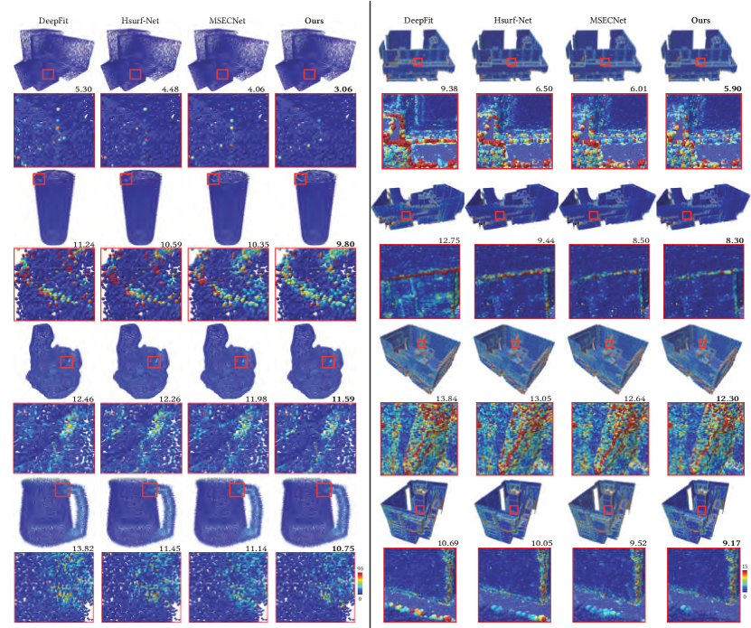
Figure 5: Qualitative comparisons of normal estimation on the PCPNet and SceneNN dataset. The values below each model indicate the RMSE deviation.

Quantitative and Qualitative Results. We perform a comprehensive comparative analysis on the PCPNet datasets between our method and various competitors encompassing both traditional and learning-based approaches for normal estimation. As summarized in Table 1, our method surpasses the previously top-performing approach by a significant margin in terms of RMSE. Under noise-free conditions, we achieve a significant improvement of 11.20% in RMSE, demonstrating our method’s enhanced ability to capture the intrinsic properties of point clouds. For non-uniform sampling, we also achieve over 10% improvement. Notably, the training data does not include non-uniform sampling data, which shows the generalization ability of our algorithm. Additionally, our method delivers state-of-the-art results in different noise conditions. On average, we improve RMSE by 4% on the PCPNet dataset, by 2.67% on the SceneNN dataset, and 2.44% on the FamousShape dataset (shown in Appendix C).

Fig. 6 presents the corresponding results using the PGP metric on the PCPNet dataset. The results further validate the significant advantages of our method compared to previous approaches. We present qualitative comparisons in Fig. 5. From which, it can be seen that our method significantly outperforms previous methods in handling complex details, sharp edges, and boundaries in challenging scenarios.

Timings. Next, we compare the efficiency of various approaches on the PCPNet dataset. Fig. 8 highlights the advantages of three different versions of our model, by plotting inference time, parameter count, and accuracy (RMSE) in one figure. Ours fast represents a version of $n{{}_{\mathrm{E}(3)}}=1$ and without GeoPatch. Ours small represents a version of $n{{}_{\mathrm{E}(3)}}=1$, $d_{fused}=256$ and without GeoPatch. Ours stands as the default version, utilizing GeoPatch. It is noteworthy that all three versions excel in terms of accuracy compared to previous methods. The complete version exhibits the most significant improvement in accuracy. Moreover, the fast version displays considerable enhancements in both accuracy and speed. Meanwhile, the small version, despite having fewer parameters than previous methods, still stands out for its remarkable speed and precision.

Table 2: Ablation studies on the PCPNet dataset. Our default setting achieves the best average result.

Ablation Noise $\sigma$ Density Average $\Delta$ None $0.12\%$ $0.6\%$ $1.2\%$ Stripes Gradient Default $N=1400$, $d_{fused}=1024$, $n{{}_{\mathrm{E}(3)}}=8$, w/ $\mathcal{L}_{\text{Gaussian}}$, w/ GeoPatch, w/ HalfPatch, w/ GaussianPatch, w/ Random Frame 3.41 8.54 15.72 20.62 3.89 4.05 9.37 - (a) w/ Random Frame, $d_{fused}=128$ 3.75 8.56 15.85 20.74 4.42 4.50 9.64 -0.27 w/o Random Frame, $d_{fused}=128$ 4.49 8.71 16.04 20.91 5.28 5.25 10.11 -0.74 (b) $n{{}_{\mathrm{E}(3)}}=4$ 3.41 8.56 15.71 20.64 3.93 4.09 9.39 -0.02 $n{{}_{\mathrm{E}(3)}}=2$ 3.48 8.56 15.75 20.64 3.94 4.11 9.41 -0.04 $n{{}_{\mathrm{E}(3)}}=1$ 3.51 8.61 15.78 20.68 3.97 4.16 9.45 -0.08 (c) w/ $\mathcal{L}^{Val}$ 3.48 8.50 15.78 20.64 4.02 4.20 9.44 -0.07 w/ $\mathcal{L}^{Half}$ 3.52 8.50 15.68 20.69 4.33 4.15 9.48 -0.11 (d) w/o GeoPatch 3.45 8.52 15.74 20.61 3.96 4.12 9.40 -0.03 w/o HalfPatch 3.50 8.66 15.90 20.81 4.06 4.16 9.52 -0.15 w/o GaussianPatch 3.43 8.55 15.73 20.63 3.91 4.07 9.39 -0.02 (e) $N=700$ 3.37 8.53 15.74 20.96 3.87 3.98 9.41 -0.04 $N=2100$ 3.47 8.56 15.79 20.63 3.98 4.09 9.42 -0.05 (f) $d_{fused}=512$ 3.50 8.49 15.70 20.70 4.10 4.21 9.45 -0.08 $d_{fused}=256$ 3.66 8.57 15.71 20.70 4.30 4.44 9.56 -0.19

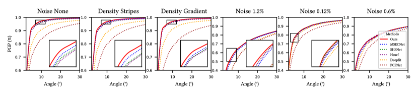
Figure 6: Statistics of the PGP results on the PCPNet dataset.

Figure 7: Comparative analysis of runtime and angle RMSE error across different methods with circle size indicating the model parameters. Figure 8: Comparisons of surface reconstruction. The values are the Hausdorff distance to the ground truth surface.

5.2 Ablation Studies

In this part, we perform ablation studies to validate various components of our model and assess their impact on performance.

(a) Random Frame Strategy. To demonstrate the efficacy of our algorithm’s random strategy from Sec. 4.1, we utilize a configuration with setting feature fusion dimension ($d_{fused}$) 128, and compare it against Puny et al. [23], which does not employ the random strategy. With the same parameter settings, replacing the random strategy with Puny et al. [23] requires eight times more training resources and results in 3.8% worse RMSE. With the same training resources, compared to our complete model, Puny et al. [23] shows an accuracy decrease of 7.9%. These results clearly illustrate that our Random Strategy significantly surpasses Puny et al. [23] in terms of both accuracy and efficiency.

(b) Frame Element Selection. As reported in Table 2, experiments reveal that using a larger number of randomly selected elements from the frame set during inference leads to improved performance. This finding implies the significance of E(3) in enhancing the efficacy of our model.

(c) Loss Function Variation. To verify the superiority of our loss function, we introduce a new function, $\mathcal{L}^{Half}$, which focuses the optimization on the nearest half of the points in a patch. $\mathcal{L}^{Val}$ means equal optimization across all points. While $\mathcal{L}^{Half}$ shows advancements in scenarios with medium noise, it is less effective compared to $\mathcal{L}^{Val}$, particularly with a 0.31 decrease in Stripes. This limitation is attributed to $\mathcal{L}^{Half}$’s limited utilization of information from unevenly sampled patches. This contrast emphasizes the strength of our Gaussian weighting approach, which optimizes neighborhood information more effectively.

(d) Configuration Removal. We remove key configurations including GeoPatch (geodesic patching), Half Sampling (discarded boundary points), and GaussianPatch (Gaussian weighted sampling) to evaluate their impacts. The results presented in Table 2 confirm the effectiveness of each component in our inference strategy.

(e) Patch Size. We also evaluate various patch sizes. Results reveal that the optimal patch size for efficient and effective noise and density handling is 1400.

(f) Feature Fusion Dimension Adjustment. By altering $d_{fused}$, we observe a clear relationship between the number of parameters and model performance. This experiment highlights the impact of the feature fusion dimension on the overall performance of the model.

5.3 Applications

We demonstrate the effectiveness of E³-Net via Poisson surface reconstruction [2] (Fig. 8). As observed in Fig. 8, our approach excels in challenging regions, including model tips and intersections, showcasing its ability to capture intricate surface structures. We also demonstrate the versatility of our proposed framework by applying random frame and frame averaging techniques to point cloud denoising (please refer to the Appendix E for more details).

6 Conclusions, Limitations, and Future Work

We presented a novel method that guarantees E(3)-equivariance for normal estimation in point clouds. Our approach effectively balances high-quality results and efficiency by combining random frame training with average frame inference. Moreover, we leverage a Gaussian weighted loss, geodesic patches, and receptive-aware weighting to enhance local feature aggregation, resulting in impressive performance. Our method outperforms competitors by a remarkable margin on three datasets and demonstrates the capability to address practical applications.

While Ours small version stands out as the fastest, smallest, and most accurate among all previous algorithms, it still exhibits some limitations compared to our complete version. Although our method achieves state-of-the-art results on real-world data, it only relies on synthetic data for training. In the future, constructing larger real-world datasets with various scanning noises and developing better simulators for real-world scanners could be beneficial. By training on better synthetic data and fine-tuning on real data, the performance could be further enhanced. Additionally, the proposed method is also adaptable for various patch-based point cloud analysis tasks, such as point cloud resampling, point cloud completion, and curvature estimation.

Broader Impact. Our algorithm addresses a fundamental problem in geometry processing, making it applicable to various domains such as point cloud denoising and surface reconstruction. As a low-level building block, our work has no direct negative societal impacts.

Appendix

Appendix A Theoretical Proof

In the following section, we present a theoretical proof to substantiate Frame Avereage in $\mathbb{R}^{3}$, which is more concise compared to Puny et al. [23].

Theorem 1.

Let $\mathbf{x}\in\mathbb{R}^{m\times 3}$ be an input point patch and $f\in\mathrm{E}(3)$ be an operation. Then the function $\Phi$ defined in Eq. 5 satisfies

$$\Phi(f(\mathbf{x}))=f\Phi(\mathbf{x})$$ (12)

Proof.

Assume $\mathscr{F}(\mathbf{x})$ is defined as follows:

$$\mathscr{F}(\mathbf{x}) =\left\{\left([\pm\boldsymbol{v}_{1},\pm\boldsymbol{v}_{2},\pm\boldsymbol{v}_{3}],\boldsymbol{t}\right)\right\}$$ (13)

$$=\{(\mathbf{U}\mathbf{T}_{i},t)\mid\mathbf{x}=\mathbf{U}\Lambda\mathbf{V}^{\top},\mathbf{t}=\frac{1}{m}\mathbf{x}^{\top}\mathbf{1}_{m\times 1},\mathbf{T}_{i}\in\mathrm{D}\}.$$ (14)

where $\mathbf{U\Lambda V^{\top}}$ is the singular value decomposition of the matrix $\mathbf{x}$, $\mathbf{D}=\{[\pm\boldsymbol{v}_{1},\pm\boldsymbol{v}_{2},\pm\boldsymbol{v}_{3}]\}$and $\mathbf{t}$ is the mean of $\mathbf{x}$ along its second dimension.

Next, assume a spatial transformation $f=(\mathbf{U}_{1},\mathbf{t}_{1})\in\mathrm{E}(3)$. When applying $f$ to $\mathbf{x}$, $\mathscr{F}(\mathbf{x})$ is modified to $\mathscr{F}(f(\mathbf{x}))$, resulting in:

$$\mathscr{F}(f(\mathbf{x}))=\left\{(\mathbf{U}_{1}\mathbf{UT}_{i},\mathbf{t}_{1}+\mathbf{t})\right\}$$

For the calculation of $\Phi(f(\mathbf{x}))$, the function $\Phi$ applied to $f(\mathbf{x})$ is defined as:

$$\Phi(f(\mathbf{x}))=\frac{1}{|\mathcal{F}(f(\mathbf{x}))|}\sum_{g_{i}\in\mathscr{F}(f(\mathbf{x}))}g_{i}\phi(g_{i}^{-1}f(\mathbf{x}))$$

Substituting the above definitions into $\Phi(f(\mathbf{x}))$ we get:

$$\Phi(f(\mathbf{x})) =\frac{1}{8}\sum_{\mathbf{T}_{i}\in\mathrm{D}}\left(\mathbf{U}_{1}\mathbf{U}\mathbf{T}_{i},\mathbf{t}_{1}+\mathbf{t}\right)\phi\left(\left(\mathbf{T}_{i}\mathbf{U}^{\top}\mathbf{U}_{1}^{\top},-\mathbf{t_{1}}-\mathbf{t}\right)\left(\mathbf{U}_{1},\mathbf{t}_{1}\right)(\mathbf{x})\right)$$ (15)

$$=\frac{1}{8}\sum_{\mathbf{T}_{i}\in\mathrm{D}}\left(\mathbf{U}_{1},\mathbf{t}_{1}\right)\left(\mathbf{UT}_{i},\mathbf{t}\right)\phi\left(\left(\mathbf{T}_{i}\mathbf{U}^{\top},-\mathbf{t}\right)(\mathbf{x})\right)$$ (16)

$$=\frac{1}{8}\sum_{\mathbf{T}_{i}\in\mathrm{D}}fg_{i}\phi(g_{i}^{-1}(\mathbf{x}))$$ (17)

$$=f\frac{1}{|\mathcal{F}(\mathbf{x})|}\sum_{g_{i}\in\mathscr{F}(\mathbf{x})}g_{i}\phi(g_{i}^{-1}(\mathbf{x}))$$ (18)

$$=f\Phi(\mathbf{x})$$ (19)

This concludes the proof. ∎

Appendix B Details of the Used Datasets

We give a detailed description of the used datasets in the paper.

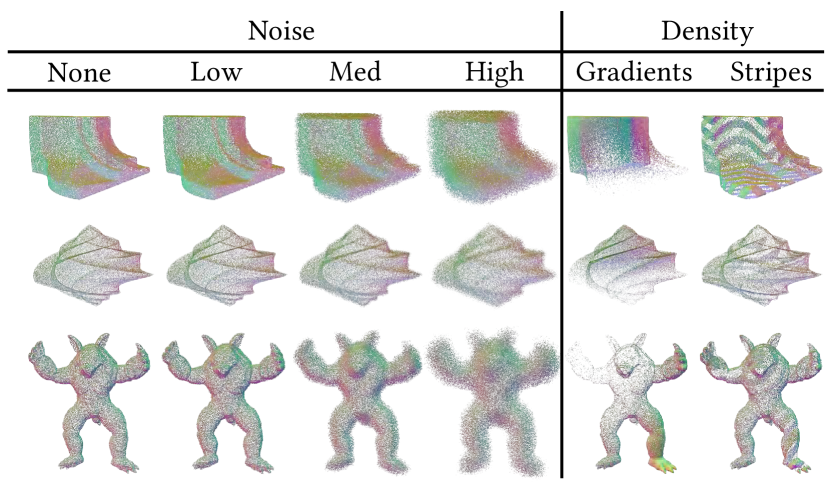
Figure 9: Examples of point clouds from the PCPNet Dataset.

PCPNet. The PCPNet dataset [14] is divided into three sets: training, validation, and test sets. The training set comprises eight models, each available in noise-free, high, medium, and low noise versions, resulting in a total of 32 point clouds with consistent density. The validation set consists of three models, each available in noise-free, high, medium, and low noise versions, as well as stripes and gradient variable density versions, resulting in a total of 18 point clouds. The test set applies these transformations to 18 models, resulting in a total of 108 point clouds for evaluation. Fig. 9 presents several illustrative examples from PCPNet dataset.

Table 3: Quantitative comparisons of normal estimation on the FamousShape dataset. Bold fonts indicate the top performer.

Method Year FamousShape Dataset Noise $\sigma$ Density Average None $0.12\%$ $0.6\%$ $1.2\%$ Stripes Gradient Jet [8] 2005 20.11 20.57 31.34 45.19 18.82 18.69 25.79 PCA [7] 1992 19.90 20.60 31.33 45.00 19.84 18.54 25.87 PCPNet [14] 2018 24.71 28.00 40.26 49.78 25.98 26.12 32.47 Nesti-Net [28] 2019 11.60 16.80 31.61 39.22 12.33 11.77 20.55 Lenssen et al. [29] 2020 11.62 16.97 30.62 39.43 11.21 10.76 20.10 DeepFit [15] 2020 11.21 16.39 29.84 39.95 11.84 10.54 19.96 Zhang et al. [31] 2022 9.83 16.13 29.81 39.81 9.72 9.19 19.08 AdaFit [16] 2021 9.09 15.78 29.78 38.74 8.52 8.57 18.41 GraphFit [17] 2022 8.91 15.73 29.37 38.67 9.10 8.62 18.40 NeAF [33] 2023 7.67 15.67 29.75 38.76 7.22 7.47 17.76 HSurf-Net [18] 2022 7.59 15.64 29.43 38.54 7.63 7.40 17.70 NGLO [34] 2023 7.25 15.60 29.35 38.74 7.60 7.20 17.62 SHS-Net [19] 2023 7.41 15.34 29.33 38.56 7.74 7.28 17.61 MSECNet [20] 2023 6.86 15.54 29.24 38.16 6.64 6.71 17.19 Ours - 6.45 15.03 28.76 37.75 6.31 6.30 16.77 Improvement 5.98%$\uparrow$ 2.02%$\uparrow$ 1.64%$\uparrow$ 1.07%$\uparrow$ 4.97%$\uparrow$ 6.11%$\uparrow$ 2.44%$\uparrow$

FamousShape. In comparison to the PCPNet dataset, the FamousShape dataset [19] incorporates more intricate structures obtained from various public datasets, such as the Famous dataset [48] and the Stanford 3D Scanning Repository [49]. The FamousShape dataset undergoes the same preprocessing steps as the PCPNet dataset to introduce data contamination.

SceneNN. SceneNN is a real-world dataset that comprises both clean and noisy scenes sourced from SceneNN [50], prepared by [18].

Appendix C Assessments on the FamousShape Dataset

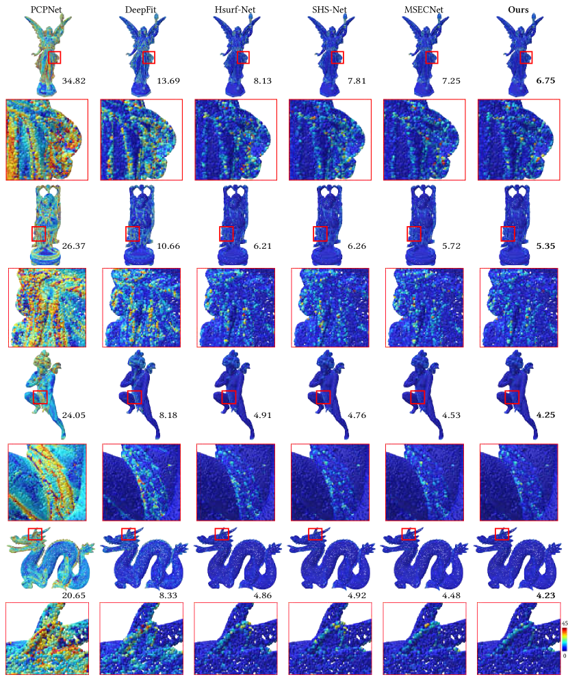
Figure 10: Qualitative comparisons of normal estimation on the FamousShape dataset. The values below each model indicate the RMSE deviation.

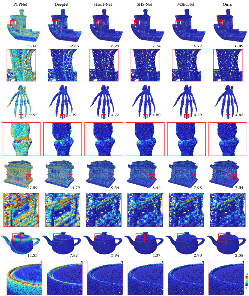
Figure 11: Qualitative comparisons of normal estimation on the FamousShape dataset. The values below each model indicate the RMSE deviation.

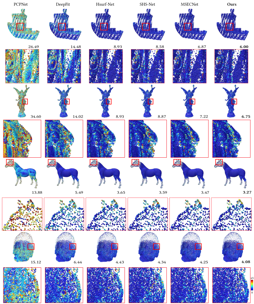
Figure 12: Qualitative comparisons of normal estimation of non-uniform density point clouds in the FamousShape dataset. The values below each model indicate the RMSE deviation.

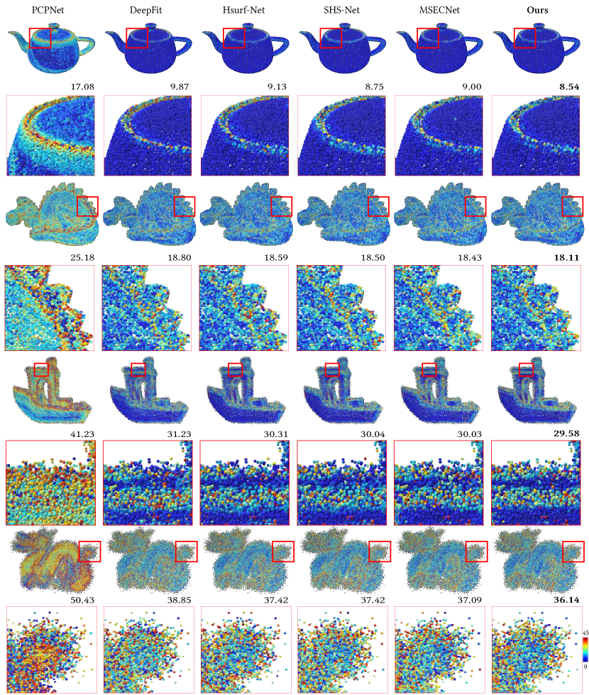
Figure 13: Qualitative comparisons of normal estimation of noisy point clouds in the FamousShape dataset. The values below each model indicate the RMSE deviation.

In our paper, we have conducted a thorough evaluation of the proposed algorithm under various conditions. Additionally, we have performed assessments on the more challenging FamousShape dataset. When evaluated under noise-free and uniform sampling settings, as depicted in Figs. 10-11, the algorithm demonstrates significant improvements in processing complex human and animal models. Notably, enhancements can be observed in intricate aspects such as clothing folds in the Happy, Angel, and Lucy models, as well as the fine edges of the dragon’s ears, highlighting the algorithm’s ability to handle detailed structures effectively.

In gradient sampling scenarios, as depicted in Fig. 12, the proposed algorithm demonstrates exceptional capability, particularly in regions with noticeable variations in sampling density, as exemplified by the Serapis model. It significantly enhances finer details, such as the ears of the Horse model and the sparsely covered head. These results highlight the algorithm’s precision and effectiveness in handling challenging gradient sampling scenarios. Additionally, in the case of stripe sampling, as illustrated in Fig. 12, the algorithm successfully handles complex areas such as Benchy’s wall surfaces and the sparsely covered skirt, demonstrating consistent performance and accuracy even in challenging conditions.

Lastly, in challenging noisy environments, as depicted in Fig. 13, the algorithm effectively handles intricate areas, including the edges of the teapot, the protrusions on the dragon’s back, the edges of Benchy, and the tail of the dragon. These results affirm the algorithm’s resilience and efficiency in managing detailed and challenging regions under different sampling and noise conditions.

Appendix D Algorithm

To enhance the comprehensibility of our developed algorithm for normal estimation, we also present the pseudo code in Algorithm 1.

Algorithm 1 Pseudo code of the proposed normal estimation algorithm

0:  Point Cloud $P$

0:  Normal $N$ of $P$

1:  $K\leftarrow\text{InitializeKDTree}(P)$

2:  $G\leftarrow\text{ConstructGraph}(P,K)$

3:  $C\leftarrow\emptyset$, $W\leftarrow\emptyset$, $N_{temp}\leftarrow\emptyset$, $N_{patch}\leftarrow\emptyset$, $N_{final}\leftarrow\emptyset$

4:  while $C\neq P$ do

5:     $q\leftarrow\text{SelectUncoveredPoint}(P,C)$

6:     if $q$ not in independent cluster then

7:        $p\leftarrow\text{ConstructPatchDijkstra}(q,G)$

8:     else

9:        $p\leftarrow\text{ConstructPatchKNN}(q,K)$

10:     end if

11:     Add points in $p$ close to the center to $C$

12:     $N_{temp}\leftarrow\emptyset$

13:     for each orientation in Frame do

14:        $p_{aligned}\leftarrow\text{FrameTransform}(p)$

15:        $n_{out}\leftarrow\text{Network}(p_{aligned})$

16:        $n\leftarrow\text{FrameInverseTransform}(n_{out})$

17:        $N_{temp}\leftarrow N_{temp}\cup{n}$

18:     end for

19:     Sort $p$ based on distance to $q$

20:     $p_{half}\leftarrow$ Nearest half of $p$ to $q$

21:     $N_{patch}\leftarrow N_{patch}\cup\{\text{mean}(N_{temp})\}$

22:     $W\leftarrow W\cup\{\text{GaussianWeights}(p_{half},q)\}$

23:  end while

24:  for each $i$ in $P$ do

25:     $N_{i}\leftarrow\text{CalculateFinalNormal}(i,N_{patch},W)$

26:     $N_{final}\leftarrow N_{final}\cup\{N_{i}\}$

27:  end for

28:  return  $N_{final}$

Appendix E Point Cloud Denoising

To validate the capability of our proposed approach, which combines random frame training with average frame inference, we also apply our framework to point cloud denoising. We utilize the current state-of-the-art algorithm, IterativePFN [51], as the backbone and conduct training and testing on the benchmark PUNet [52] dataset. We use Chamfer distance (CD) and the Point2Mesh distance (P2M) as evaluation metrics to measure the denoising effects. All the result metrics are multiplied by $10^{5}$. IterativePFN employs a strategy of random rotation during training for data augmentation. Our improvement is to apply our random frame training strategy during training and utilize the average frame strategy during inference. The results, as shown in Table 4 and Fig. 14, reveal that our algorithm outperforms IterativePFN in various scenarios, including point clouds of densities 10k and 50k, and noise levels of 1%, 2%, and 2.5%. As demonstrated in Fig. 14, our algorithm exhibits improvements in both sharp edges and flat surfaces.

Our random frame strategy surpasses conventional random rotation training by eliminating the need for the network to learn from point cloud patches in all poses. Instead, it selectively uses the frame set for training, resulting in higher accuracy and better data utilization. This method is more efficient and effective for point cloud learning compared to previous random rotation approaches.

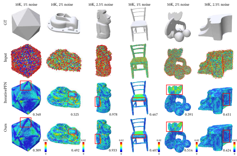
Figure 14: Qualitative comparisons of point cloud denoising on the PUNet dataset. The values below each model indicate the Point2Mesh distance (P2M). The numbers above each column represent the size of the point cloud and the noise level.

Table 4: Quantitative comparisons of point cloud denoising on the PUNet dataset. Bold fonts indicate the top performer.

Method $10K$ points $50K$ points $1\%$ noise $2\%$ noise $2.5\%$ noise $1\%$ noise $2\%$ noise $2.5\%$ noise CD P2M CD P2M CD P2M CD P2M CD P2M CD P2M Noisy 36.9 16.03 79.39 47.72 105.02 70.03 18.69 12.82 50.48 41.36 72.49 62.03 PCN [53] 36.86 15.99 79.26 47.59 104.86 69.87 11.03 6.46 19.78 13.7 32.03 24.86 GPDNet [54] 23.1 7.14 42.84 18.55 58.37 30.66 10.49 6.35 32.88 25.03 50.85 41.34 DMRDenoise [55] 47.12 21.96 50.85 25.23 52.77 26.69 12.05 7.62 14.43 9.7 16.96 11.9 PDFlow [56] 21.26 6.74 32.46 13.24 36.27 17.02 6.51 4.16 12.7 9.21 18.74 14.26 ScoreDenoise [57] 25.22 7.54 36.83 13.8 42.32 19.04 7.16 4.0 12.89 8.33 14.45 9.58 Pointfilter [58] 24.61 7.3 35.34 11.55 40.99 15.05 7.58 4.32 9.07 5.07 10.99 6.29 IterativePFN [51] 20.56 5.01 30.43 8.45 33.52 10.45 6.05 3.02 8.03 4.36 10.15 5.88 Ours 19.87 4.93 29.99 8.18 33.03 10.11 5.92 2.94 7.78 4.22 9.93 5.78

NeurIPS Paper Checklist

1. Claims

2. Question: Do the main claims made in the abstract and introduction accurately reflect the paper’s contributions and scope?

3. Answer: [Yes]

4. Justification: The main claims made in the abstract and introduction, including the efficient E(3)-equivariant method, the Gaussian weight loss function, and receptive-aware inference strategies, accurately reflect the paper’s contributions and scope.

5. Guidelines:

   • The answer NA means that the abstract and introduction do not include the claims made in the paper.

   • The abstract and/or introduction should clearly state the claims made, including the contributions made in the paper and important assumptions and limitations. A No or NA answer to this question will not be perceived well by the reviewers.

   • The claims made should match theoretical and experimental results, and reflect how much the results can be expected to generalize to other settings.

   • It is fine to include aspirational goals as motivation as long as it is clear that these goals are not attained by the paper.

6. Limitations

7. Question: Does the paper discuss the limitations of the work performed by the authors?

8. Answer: [Yes]

9. Justification: The paper discusses limitations in the conclusions section, such as its reliance on synthetic data for training, which could be mitigated by incorporating real-world data and improved simulators.

10. Guidelines:

    • The answer NA means that the paper has no limitation while the answer No means that the paper has limitations, but those are not discussed in the paper.

    • The authors are encouraged to create a separate "Limitations" section in their paper.

    • The paper should point out any strong assumptions and how robust the results are to violations of these assumptions (e.g., independence assumptions, noiseless settings, model well-specification, asymptotic approximations only holding locally). The authors should reflect on how these assumptions might be violated in practice and what the implications would be.

    • The authors should reflect on the scope of the claims made, e.g., if the approach was only tested on a few datasets or with a few runs. In general, empirical results often depend on implicit assumptions, which should be articulated.

    • The authors should reflect on the factors that influence the performance of the approach. For example, a facial recognition algorithm may perform poorly when image resolution is low or images are taken in low lighting. Or a speech-to-text system might not be used reliably to provide closed captions for online lectures because it fails to handle technical jargon.

    • The authors should discuss the computational efficiency of the proposed algorithms and how they scale with dataset size.

    • If applicable, the authors should discuss possible limitations of their approach to address problems of privacy and fairness.

    • While the authors might fear that complete honesty about limitations might be used by reviewers as grounds for rejection, a worse outcome might be that reviewers discover limitations that aren’t acknowledged in the paper. The authors should use their best judgment and recognize that individual actions in favor of transparency play an important role in developing norms that preserve the integrity of the community. Reviewers will be specifically instructed to not penalize honesty concerning limitations.

11. Theory Assumptions and Proofs

12. Question: For each theoretical result, does the paper provide the full set of assumptions and a complete (and correct) proof?

13. Answer: [Yes]

14. Justification: The theoretical aspects are thoroughly detailed, with all necessary assumptions and proofs provided in the appendix.

15. Guidelines:

    • The answer NA means that the paper does not include theoretical results.

    • All the theorems, formulas, and proofs in the paper should be numbered and cross-referenced.

    • All assumptions should be clearly stated or referenced in the statement of any theorems.

    • The proofs can either appear in the main paper or the supplemental material, but if they appear in the supplemental material, the authors are encouraged to provide a short proof sketch to provide intuition.

    • Inversely, any informal proof provided in the core of the paper should be complemented by formal proofs provided in appendix or supplemental material.

    • Theorems and Lemmas that the proof relies upon should be properly referenced.

16. Experimental Result Reproducibility

17. Question: Does the paper fully disclose all the information needed to reproduce the main experimental results of the paper to the extent that it affects the main claims and/or conclusions of the paper (regardless of whether the code and data are provided or not)?

18. Answer: [Yes]

19. Justification: The paper includes detailed descriptions of the datasets, model architectures, training parameters, and evaluation metrics to ensure reproducibility.

20. Guidelines:

    • The answer NA means that the paper does not include experiments.

    • If the paper includes experiments, a No answer to this question will not be perceived well by the reviewers: Making the paper reproducible is important, regardless of whether the code and data are provided or not.

    • If the contribution is a dataset and/or model, the authors should describe the steps taken to make their results reproducible or verifiable.

    • Depending on the contribution, reproducibility can be accomplished in various ways. For example, if the contribution is a novel architecture, describing the architecture fully might suffice, or if the contribution is a specific model and empirical evaluation, it may be necessary to either make it possible for others to replicate the model with the same dataset, or provide access to the model. In general. releasing code and data is often one good way to accomplish this, but reproducibility can also be provided via detailed instructions for how to replicate the results, access to a hosted model (e.g., in the case of a large language model), releasing of a model checkpoint, or other means that are appropriate to the research performed.

    • While NeurIPS does not require releasing code, the conference does require all submissions to provide some reasonable avenue for reproducibility, which may depend on the nature of the contribution. For example

      1. If the contribution is primarily a new algorithm, the paper should make it clear how to reproduce that algorithm.

      2. If the contribution is primarily a new model architecture, the paper should describe the architecture clearly and fully.

      3. If the contribution is a new model (e.g., a large language model), then there should either be a way to access this model for reproducing the results or a way to reproduce the model (e.g., with an open-source dataset or instructions for how to construct the dataset).

      4. We recognize that reproducibility may be tricky in some cases, in which case authors are welcome to describe the particular way they provide for reproducibility. In the case of closed-source models, it may be that access to the model is limited in some way (e.g., to registered users), but it should be possible for other researchers to have some path to reproducing or verifying the results.

21. Open access to data and code

22. Question: Does the paper provide open access to the data and code, with sufficient instructions to faithfully reproduce the main experimental results, as described in supplemental material?

23. Answer: [Yes]

24. Justification: We provide our code with sufficient instructions to reproduce the main experimental results. Both the training and testing code are included in the supplemental material.

25. Guidelines:

    • The answer NA means that paper does not include experiments requiring code.

    • Please see the NeurIPS code and data submission guidelines (https://nips.cc/public/guides/CodeSubmissionPolicy) for more details.

    • While we encourage the release of code and data, we understand that this might not be possible, so “No” is an acceptable answer. Papers cannot be rejected simply for not including code, unless this is central to the contribution (e.g., for a new open-source benchmark).

    • The instructions should contain the exact command and environment needed to run to reproduce the results. See the NeurIPS code and data submission guidelines (https://nips.cc/public/guides/CodeSubmissionPolicy) for more details.

    • The authors should provide instructions on data access and preparation, including how to access the raw data, preprocessed data, intermediate data, and generated data, etc.

    • The authors should provide scripts to reproduce all experimental results for the new proposed method and baselines. If only a subset of experiments are reproducible, they should state which ones are omitted from the script and why.

    • At submission time, to preserve anonymity, the authors should release anonymized versions (if applicable).

    • Providing as much information as possible in supplemental material (appended to the paper) is recommended, but including URLs to data and code is permitted.

26. Experimental Setting/Details

27. Question: Does the paper specify all the training and test details (e.g., data splits, hyperparameters, how they were chosen, type of optimizer, etc.) necessary to understand the results?

28. Answer: [Yes]

29. Justification: All relevant details regarding the training and testing setups, including data splits, hyperparameters, and optimizers, are provided in the experimental results section and supplementary material.

30. Guidelines:

    • The answer NA means that the paper does not include experiments.

    • The experimental setting should be presented in the core of the paper to a level of detail that is necessary to appreciate the results and make sense of them.

    • The full details can be provided either with the code, in appendix, or as supplemental material.

31. Experiment Statistical Significance

32. Question: Does the paper report error bars suitably and correctly defined or other appropriate information about the statistical significance of the experiments?

33. Answer: [No]

34. Justification: The paper does not include error bars or statistical significance tests for the experimental results, focusing instead on overall performance metrics.

35. Guidelines:

    • The answer NA means that the paper does not include experiments.

    • The authors should answer "Yes" if the results are accompanied by error bars, confidence intervals, or statistical significance tests, at least for the experiments that support the main claims of the paper.

    • The factors of variability that the error bars are capturing should be clearly stated (for example, train/test split, initialization, random drawing of some parameter, or overall run with given experimental conditions).

    • The method for calculating the error bars should be explained (closed form formula, call to a library function, bootstrap, etc.)

    • The assumptions made should be given (e.g., Normally distributed errors).

    • It should be clear whether the error bar is the standard deviation or the standard error of the mean.

    • It is OK to report 1-sigma error bars, but one should state it. The authors should preferably report a 2-sigma error bar than state that they have a 96% CI, if the hypothesis of Normality of errors is not verified.

    • For asymmetric distributions, the authors should be careful not to show in tables or figures symmetric error bars that would yield results that are out of range (e.g. negative error rates).

    • If error bars are reported in tables or plots, The authors should explain in the text how they were calculated and reference the corresponding figures or tables in the text.

36. Experiments Compute Resources

37. Question: For each experiment, does the paper provide sufficient information on the computer resources (type of compute workers, memory, time of execution) needed to reproduce the experiments?

38. Answer: [Yes]

39. Justification: The paper specifies the use of NVIDIA 4090 GPUs, detailing the training details and batch sizes, thereby providing sufficient information on the compute resources used.

40. Guidelines:

    • The answer NA means that the paper does not include experiments.

    • The paper should indicate the type of compute workers CPU or GPU, internal cluster, or cloud provider, including relevant memory and storage.

    • The paper should provide the amount of compute required for each of the individual experimental runs as well as estimate the total compute.

    • The paper should disclose whether the full research project required more compute than the experiments reported in the paper (e.g., preliminary or failed experiments that didn’t make it into the paper).

41. Code Of Ethics

42. Question: Does the research conducted in the paper conform, in every respect, with the NeurIPS Code of Ethics https://neurips.cc/public/EthicsGuidelines?

43. Answer: [Yes]

44. Justification: The research aligns with the NeurIPS Code of Ethics, ensuring transparency, reproducibility, and consideration of ethical implications.

45. Guidelines:

    • The answer NA means that the authors have not reviewed the NeurIPS Code of Ethics.

    • If the authors answer No, they should explain the special circumstances that require a deviation from the Code of Ethics.

    • The authors should make sure to preserve anonymity (e.g., if there is a special consideration due to laws or regulations in their jurisdiction).

46. Broader Impacts

47. Question: Does the paper discuss both potential positive societal impacts and negative societal impacts of the work performed?

48. Answer: [Yes]

49. Justification: We have presented a paragraph to discuss the broader impacts of our work. The paper focuses on a fundamental geometry process task, and thus there is no direct negative societal impacts of the work performed.

50. Guidelines:

    • The answer NA means that there is no societal impact of the work performed.

    • If the authors answer NA or No, they should explain why their work has no societal impact or why the paper does not address societal impact.

    • Examples of negative societal impacts include potential malicious or unintended uses (e.g., disinformation, generating fake profiles, surveillance), fairness considerations (e.g., deployment of technologies that could make decisions that unfairly impact specific groups), privacy considerations, and security considerations.

    • The conference expects that many papers will be foundational research and not tied to particular applications, let alone deployments. However, if there is a direct path to any negative applications, the authors should point it out. For example, it is legitimate to point out that an improvement in the quality of generative models could be used to generate deepfakes for disinformation. On the other hand, it is not needed to point out that a generic algorithm for optimizing neural networks could enable people to train models that generate Deepfakes faster.

    • The authors should consider possible harms that could arise when the technology is being used as intended and functioning correctly, harms that could arise when the technology is being used as intended but gives incorrect results, and harms following from (intentional or unintentional) misuse of the technology.

    • If there are negative societal impacts, the authors could also discuss possible mitigation strategies (e.g., gated release of models, providing defenses in addition to attacks, mechanisms for monitoring misuse, mechanisms to monitor how a system learns from feedback over time, improving the efficiency and accessibility of ML).

51. Safeguards

52. Question: Does the paper describe safeguards that have been put in place for responsible release of data or models that have a high risk for misuse (e.g., pretrained language models, image generators, or scraped datasets)?

53. Answer: [N/A]

54. Justification: The paper does not involve the release of high-risk data or models that would require special safeguards.

55. Guidelines:

    • The answer NA means that the paper poses no such risks.

    • Released models that have a high risk for misuse or dual-use should be released with necessary safeguards to allow for controlled use of the model, for example by requiring that users adhere to usage guidelines or restrictions to access the model or implementing safety filters.

    • Datasets that have been scraped from the Internet could pose safety risks. The authors should describe how they avoided releasing unsafe images.

    • We recognize that providing effective safeguards is challenging, and many papers do not require this, but we encourage authors to take this into account and make a best faith effort.

56. Licenses for existing assets

57. Question: Are the creators or original owners of assets (e.g., code, data, models), used in the paper, properly credited and are the license and terms of use explicitly mentioned and properly respected?

58. Answer: [Yes]

59. Justification: The paper credits all datasets and models used, including proper citations and adherence to license terms where applicable.

60. Guidelines:

    • The answer NA means that the paper does not use existing assets.

    • The authors should cite the original paper that produced the code package or dataset.

    • The authors should state which version of the asset is used and, if possible, include a URL.

    • The name of the license (e.g., CC-BY 4.0) should be included for each asset.

    • For scraped data from a particular source (e.g., website), the copyright and terms of service of that source should be provided.

    • If assets are released, the license, copyright information, and terms of use in the package should be provided. For popular datasets, paperswithcode.com/datasets has curated licenses for some datasets. Their licensing guide can help determine the license of a dataset.

    • For existing datasets that are re-packaged, both the original license and the license of the derived asset (if it has changed) should be provided.

    • If this information is not available online, the authors are encouraged to reach out to the asset’s creators.

61. New Assets

62. Question: Are new assets introduced in the paper well documented and is the documentation provided alongside the assets?

63. Answer: [N/A]

64. Justification: The paper does not introduce new assets, focusing on the development and evaluation of the proposed method.

65. Guidelines:

    • The answer NA means that the paper does not release new assets.

    • Researchers should communicate the details of the dataset/code/model as part of their submissions via structured templates. This includes details about training, license, limitations, etc.

    • The paper should discuss whether and how consent was obtained from people whose asset is used.

    • At submission time, remember to anonymize your assets (if applicable). You can either create an anonymized URL or include an anonymized zip file.

66. Crowdsourcing and Research with Human Subjects

67. Question: For crowdsourcing experiments and research with human subjects, does the paper include the full text of instructions given to participants and screenshots, if applicable, as well as details about compensation (if any)?

68. Answer: [N/A]

69. Justification: The paper does not involve crowdsourcing or research with human subjects.

70. Guidelines:

    • The answer NA means that the paper does not involve crowdsourcing nor research with human subjects.

    • Including this information in the supplemental material is fine, but if the main contribution of the paper involves human subjects, then as much detail as possible should be included in the main paper.

    • According to the NeurIPS Code of Ethics, workers involved in data collection, curation, or other labor should be paid at least the minimum wage in the country of the data collector.

71. Institutional Review Board (IRB) Approvals or Equivalent for Research with Human Subjects

72. Question: Does the paper describe potential risks incurred by study participants, whether such risks were disclosed to the subjects, and whether Institutional Review Board (IRB) approvals (or an equivalent approval/review based on the requirements of your country or institution) were obtained?

73. Answer: [N/A]

74. Justification: The paper does not involve research with human subjects, thus no IRB approval is required.

75. Guidelines:

    • The answer NA means that the paper does not involve crowdsourcing nor research with human subjects.

    • Depending on the country in which research is conducted, IRB approval (or equivalent) may be required for any human subjects research. If you obtained IRB approval, you should clearly state this in the paper.

    • We recognize that the procedures for this may vary significantly between institutions and locations, and we expect authors to adhere to the NeurIPS Code of Ethics and the guidelines for their institution.

    • For initial submissions, do not include any information that would break anonymity (if applicable), such as the institution conducting the review.

References

- [1] Michael Kazhdan, Matthew Bolitho, and Hugues Hoppe. Poisson surface reconstruction. In Symp. Geom. Process., volume 7, pages 61–70, 2006.
- [2] Michael Kazhdan and Hugues Hoppe. Screened Poisson surface reconstruction. ACM Trans. Graph., 32(3):1–13, 2013.
- [3] Bertram Drost, Markus Ulrich, Nassir Navab, and Slobodan Ilic. Model globally, match locally: Efficient and robust 3d object recognition. In Proc. IEEE Conf. Comput. Vis. Pattern Recog., pages 998–1005, 2010.
- [4] Gabriel J Brostow, Jamie Shotton, Julien Fauqueur, and Roberto Cipolla. Segmentation and recognition using structure from motion point clouds. In Proc. Eur. Conf. Comput. Vis., pages 44–57, 2008.
- [5] Shachar Fleishman, Iddo Drori, and Daniel Cohen-Or. Bilateral mesh denoising. ACM Trans. Graph., 22(3):950–953, 2003.
- [6] Haim Avron, Andrei Sharf, Chen Greif, and Daniel Cohen-Or. l1-sparse reconstruction of sharp point set surfaces. ACM Trans. Graph., 29(5):1–12, 2010.
- [7] Hugues Hoppe, Tony DeRose, Tom Duchamp, John McDonald, and Werner Stuetzle. Surface reconstruction from unorganized points. In Proc. ACM SIGGRAPH, pages 71–78, 1992.
- [8] Frédéric Cazals and Marc Pouget. Estimating differential quantities using polynomial fitting of osculating jets. Comput. Aided Geom. Des., 22(2):121–146, 2005.
- [9] David Levin. The approximation power of moving least-squares. Math. Comput., 67(224):1517–1531, 1998.
- [10] Niloy J Mitra, An Nguyen, and Leonidas Guibas. Estimating surface normals in noisy point cloud data. Int. J. Comput. Geom. Appl., 14(4), 2004.
- [11] Quentin Mérigot, Maks Ovsjanikov, and Leonidas J Guibas. Voronoi-based curvature and feature estimation from point clouds. IEEE Trans. Vis. Comput. Graph., 17(6):743–756, 2010.
- [12] Alexandre Boulch and Renaud Marlet. Fast and robust normal estimation for point clouds with sharp features. Comput. Graph. Forum, 31(5):1765–1774, 2012.
- [13] Rui Xu, Zhiyang Dou, Ningna Wang, Shiqing Xin, Shuangmin Chen, Mingyan Jiang, Xiaohu Guo, Wenping Wang, and Changhe Tu. Globally consistent normal orientation for point clouds by regularizing the winding-number field. ACM Trans. Graph., 42(4):1–15, 2023.
- [14] Paul Guerrero, Yanir Kleiman, Maks Ovsjanikov, and Niloy J Mitra. PCPNet: learning local shape properties from raw point clouds. Comput. Graph. Forum, 37(2):75–85, 2018.
- [15] Yizhak Ben-Shabat and Stephen Gould. DeepFit: 3D surface fitting via neural network weighted least squares. In Proc. Eur. Conf. Comput. Vis., pages 20–34, 2020.
- [16] Runsong Zhu, Yuan Liu, Zhen Dong, Yuan Wang, Tengping Jiang, Wenping Wang, and Bisheng Yang. AdaFit: Rethinking learning-based normal estimation on point clouds. In Proc. IEEE Int. Conf. Comput. Vis., pages 6118–6127, 2021.
- [17] Keqiang Li, Mingyang Zhao, Huaiyu Wu, Dong-Ming Yan, Zhen Shen, Fei-Yue Wang, and Gang Xiong. GraphFit: Learning multi-scale graph-convolutional representation for point cloud normal estimation. In Proc. Eur. Conf. Comput. Vis., pages 651–667, 2022.
- [18] Qing Li, Yu-Shen Liu, Jin-San Cheng, Cheng Wang, Yi Fang, and Zhizhong Han. HSurf-Net: Normal estimation for 3D point clouds by learning hyper surfaces. Proc. Int. Conf. Neural Inf. Process. Syst., 35:4218–4230, 2022.
- [19] Qing Li, Huifang Feng, Kanle Shi, Yue Gao, Yi Fang, Yu-Shen Liu, and Zhizhong Han. SHS-Net: Learning signed hyper surfaces for oriented normal estimation of point clouds. In Proc. IEEE Conf. Comput. Vis. Pattern Recog., pages 13591–13600, 2023.
- [20] Haoyi Xiu, Xin Liu, Weimin Wang, Kyoung-Sook Kim, and Masashi Matsuoka. MSECNet: Accurate and robust normal estimation for 3D point clouds by multi-scale edge conditioning. In Proc. ACM Int. Conf. Multimedia., pages 2535–2543, 2023.
- [21] Franco Scarselli, Marco Gori, Ah Chung Tsoi, Markus Hagenbuchner, and Gabriele Monfardini. The graph neural network model. IEEE Trans. Neural Networks, 20(1):61–80, 2008.
- [22] Charles R Qi, Hao Su, Kaichun Mo, and Leonidas J Guibas. PointNet: Deep learning on point sets for 3D classification and segmentation. In Proc. IEEE Conf. Comput. Vis. Pattern Recog., pages 652–660, 2017.
- [23] Omri Puny, Matan Atzmon, Edward J Smith, Ishan Misra, Aditya Grover, Heli Ben-Hamu, and Yaron Lipman. Frame averaging for invariant and equivariant network design. In Proc. Int. Conf. Learning Representations., 2021.
- [24] Vıctor Garcia Satorras, Emiel Hoogeboom, and Max Welling. E(n) equivariant graph neural networks. In Proc. Int. Conf. Mach. Learning., pages 9323–9332, 2021.
- [25] Antoni Buades, Bartomeu Coll, and Jean-Michel Morel. A review of image denoising algorithms, with a new one. Multiscale Model. Simul., 4(2):490–530, 2005.
- [26] Jun Zhou, Hua Huang, Bin Liu, and Xiuping Liu. Normal estimation for 3D point clouds via local plane constraint and multi-scale selection. Comput. Aided Des., 129:102916, 2020.
- [27] Junjie Cao, Hairui Zhu, Yunpeng Bai, Jun Zhou, Jinshan Pan, and Zhixun Su. Latent tangent space representation for normal estimation. IEEE Trans. Ind. Electron., 69(1):921–929, 2021.
- [28] Yizhak Ben-Shabat, Michael Lindenbaum, and Anath Fischer. Nesti-Net: Normal estimation for unstructured 3D point clouds using convolutional neural networks. In Proc. IEEE Conf. Comput. Vis. Pattern Recog., pages 10112–10120, 2019.
- [29] Jan Eric Lenssen, Christian Osendorfer, and Jonathan Masci. Deep iterative surface normal estimation. In Proc. IEEE Conf. Comput. Vis. Pattern Recog., pages 11247–11256, 2020.
- [30] Haoran Zhou, Honghua Chen, Yingkui Zhang, Mingqiang Wei, Haoran Xie, Jun Wang, Tong Lu, Jing Qin, and Xiao-Ping Zhang. Refine-net: Normal refinement neural network for noisy point clouds. IEEE Trans. Pattern Anal. Mach. Intell., 45(1):946–963, 2022.
- [31] Jie Zhang, Jun-Jie Cao, Hai-Rui Zhu, Dong-Ming Yan, and Xiu-Ping Liu. Geometry guided deep surface normal estimation. Comput. Aided Des., 142:103119, 2022.
- [32] Hang Du, Xuejun Yan, Jingjing Wang, Di Xie, and Shiliang Pu. Rethinking the approximation error in 3D surface fitting for point cloud normal estimation. In Proc. IEEE Conf. Comput. Vis. Pattern Recog., pages 9486–9495, 2023.
- [33] Shujuan Li, Junsheng Zhou, Baorui Ma, Yu-Shen Liu, and Zhizhong Han. Neaf: Learning neural angle fields for point normal estimation. In Proc. AAAI Conf. Artif. Intell., volume 37, pages 1396–1404, 2023.
- [34] Qing Li, Huifang Feng, Kanle Shi, Yi Fang, Yu-Shen Liu, and Zhizhong Han. Neural gradient learning and optimization for oriented point normal estimation. In SIGGRAPH Asia Conf. Pap., pages 122:1–122:9, 2023.
- [35] Congyue Deng, Or Litany, Yueqi Duan, Adrien Poulenard, Andrea Tagliasacchi, and Leonidas J Guibas. Vector neurons: A general framework for so (3)-equivariant networks. In Proc. IEEE Int. Conf. Comput. Vis., pages 12200–12209, 2021.
- [36] Xianzhi Li, Ruihui Li, Guangyong Chen, Chi-Wing Fu, Daniel Cohen-Or, and Pheng-Ann Heng. A rotation-invariant framework for deep point cloud analysis. IEEE Trans. Vis. Comput. Graph., 28(12):4503–4514, 2021.
- [37] Haiwei Chen, Shichen Liu, Weikai Chen, Hao Li, and Randall Hill. Equivariant point network for 3d point cloud analysis. In Proc. IEEE Conf. Comput. Vis. Pattern Recog., pages 14514–14523, 2021.
- [38] Serge Assaad, Carlton Downey, Rami Al-Rfou, Nigamaa Nayakanti, and Ben Sapp. Vn-transformer: Rotation-equivariant attention for vector neurons. arXiv preprint arXiv:2206.04176, 2022.
- [39] Carlos Esteves, Christine Allen-Blanchette, Ameesh Makadia, and Kostas Daniilidis. Learning so (3) equivariant representations with spherical cnns. In Proc. Eur. Conf. Comput. Vis., pages 52–68, 2018.
- [40] Kristof T Schütt, Huziel E Sauceda, P-J Kindermans, Alexandre Tkatchenko, and K-R Müller. Schnet–a deep learning architecture for molecules and materials. J. Chem. Phys., 148(24), 2018.
- [41] Nathaniel Thomas, Tess Smidt, Steven Kearnes, Lusann Yang, Li Li, Kai Kohlhoff, and Patrick Riley. Tensor field networks: Rotation-and translation-equivariant neural networks for 3D point clouds. arXiv preprint arXiv:1802.08219, 2018.
- [42] Jonas Köhler, Leon Klein, and Frank Noé. Equivariant flows: exact likelihood generative learning for symmetric densities. In Proc. Int. Conf. Mach. Learning., pages 5361–5370. PMLR, 2020.
- [43] Fabian Fuchs, Daniel Worrall, Volker Fischer, and Max Welling. SE(3)-transformers: 3D roto-translation equivariant attention networks. Proc. Int. Conf. Neural Inf. Process. Syst., 33:1970–1981, 2020.
- [44] Matan Atzmon, Koki Nagano, Sanja Fidler, Sameh Khamis, and Yaron Lipman. Frame averaging for equivariant shape space learning. In Proc. IEEE Conf. Comput. Vis. Pattern Recog., pages 631–641, 2022.
- [45] Ren-Wu Li, Ling-Xiao Zhang, Chunpeng Li, Yu-Kun Lai, and Lin Gao. E3Sym: Leveraging E(3) invariance for unsupervised 3D planar reflective symmetry detection. In Proc. IEEE Int. Conf. Comput. Vis., pages 14543–14553, 2023.
- [46] Alexandre Agm Duval, Victor Schmidt, Alex Hernandez-Garcia, Santiago Miret, Fragkiskos D Malliaros, Yoshua Bengio, and David Rolnick. FaeNet: Frame averaging equivariant gnn for materials modeling. In Proc. Int. Conf. Mach. Learning., pages 9013–9033. PMLR, 2023.
- [47] Ilya Loshchilov and Frank Hutter. Decoupled weight decay regularization. In Proc. Int. Conf. Learning Representations., 2018.
- [48] Philipp Erler, Paul Guerrero, Stefan Ohrhallinger, Niloy J Mitra, and Michael Wimmer. Points2surf learning implicit surfaces from point clouds. In Proc. Eur. Conf. Comput. Vis., pages 108–124, 2020.
- [49] Brian Curless and Marc Levoy. A volumetric method for building complex models from range images. In Proc. ACM SIGGRAPH, pages 303–312, 1996.
- [50] Binh-Son Hua, Quang-Hieu Pham, Duc Thanh Nguyen, Minh-Khoi Tran, Lap-Fai Yu, and Sai-Kit Yeung. SceneNN: A scene meshes dataset with annotations. In Int. Conf. 3D Vis., pages 92–101, 2016.
- [51] Dasith de Silva Edirimuni, Xuequan Lu, Zhiwen Shao, Gang Li, Antonio Robles-Kelly, and Ying He. IterativePFN: True iterative point cloud filtering. In Proc. IEEE Conf. Comput. Vis. Pattern Recog., pages 13530–13539, 2023.
- [52] Lequan Yu, Xianzhi Li, Chi-Wing Fu, Daniel Cohen-Or, and Pheng-Ann Heng. Pu-net: Point cloud upsampling network. In Proc. IEEE Conf. Comput. Vis. Pattern Recog., pages 2790–2799, 2018.
- [53] Marie-Julie Rakotosaona, Vittorio La Barbera, Paul Guerrero, Niloy J Mitra, and Maks Ovsjanikov. Pointcleannet: Learning to denoise and remove outliers from dense point clouds. In Comput. Graph. Forum, volume 39, pages 185–203. Wiley Online Library, 2020.
- [54] Francesca Pistilli, Giulia Fracastoro, Diego Valsesia, and Enrico Magli. Learning graph-convolutional representations for point cloud denoising. In Proc. Eur. Conf. Comput. Vis., pages 103–118. Springer, 2020.
- [55] Shitong Luo and Wei Hu. Differentiable manifold reconstruction for point cloud denoising. In Proc. ACM Int. Conf. Multimedia., pages 1330–1338, 2020.
- [56] Aihua Mao, Zihui Du, Yu-Hui Wen, Jun Xuan, and Yong-Jin Liu. PD-Flow: A point cloud denoising framework with normalizing flows. In Proc. Eur. Conf. Comput. Vis., pages 398–415. Springer, 2022.
- [57] Shitong Luo and Wei Hu. Score-based point cloud denoising. In Proc. IEEE Int. Conf. Comput. Vis., pages 4583–4592, 2021.
- [58] Dongbo Zhang, Xuequan Lu, Hong Qin, and Ying He. Pointfilter: Point cloud filtering via encoder-decoder modeling. IEEE Trans. Vis. Comput. Graph., 27(3):2015–2027, 2020.