Efficient Historical Butterfly Counting in Large Temporal Bipartite Networks via Graph Structure-aware Index

Abstract.

Bipartite graphs are ubiquitous in many domains, e.g., e-commerce platforms, social networks, and academia, by modeling interactions between distinct entity sets. Within these graphs, the butterfly motif, a complete 2$\times$2 biclique, represents the simplest yet significant subgraph structure, crucial for analyzing complex network patterns. Counting the butterflies offers significant benefits across various applications, including community analysis and recommender systems. Additionally, the temporal dimension of bipartite graphs, where edges activate within specific time frames, introduces the concept of historical butterfly counting, i.e., counting butterflies within a given time interval. This temporal analysis sheds light on the dynamics and evolution of network interactions, offering new insights into their mechanisms. Despite its importance, no existing algorithm can efficiently solve the historical butterfly counting task. To address this, we design two novel indices whose memory footprints are dependent on #butterflies and #wedges, respectively. Combining these indices, we propose a graph structure-aware indexing approach that significantly reduces memory usage while preserving exceptional query speed. We theoretically prove that our approach is particularly advantageous on power-law graphs, a common characteristic of real-world bipartite graphs, by surpassing traditional complexity barriers for general graphs. Extensive experiments reveal that our query algorithms outperform existing methods by up to five magnitudes, effectively balancing speed with manageable memory requirements.

1. INTRODUCTION

Due to its ability to model relationships between two distinct sets of entities, the bipartite graph, or network, holds significant importance across various fields, including disease control on people-location networks (Eubank et al., 2004a; Pavlopoulos et al., 2018), fraud detection on user-page networks (Wang et al., 2019; Liu et al., 2019b) and recommendation on customer-product networks (Wang et al., 2006; He et al., 2017, 2020; Wang et al., 2020; Wu et al., 2022). To analyze the structure and dynamics of the network, counting motifs is one of the most popular methods (Milo et al., 2002; Wang et al., 2020; Fang et al., 2020; Jha et al., 2013; Eubank et al., 2004b) since motifs are considered the basic construction block of the network. The butterfly motif ($2\times 2$ biclique) represents fundamental interaction patterns within the graph, and counting it has wide applications, ranging from biological ecosystems (Wang et al., 2019; Sanei-Mehri et al., 2018; Wang et al., 2014), where it helps in identifying mutual relationships between species, to social networks (Zou, 2016; Wang et al., 2020), where it uncovers patterns of collaborations and affiliations. On the other hand, temporal bipartite graphs, in which edges are active in a certain range of time, are often being considered (Cai et al., 2024; Chen et al., 2021; Eubank et al., 2004b; Pavlopoulos et al., 2018) since the real-world interactions (modeled as edges) are usually active on certain time windows. Recently, Cai et.al (Cai et al., 2024) first considers counting butterflies on temporal bipartite graphs, which extends the analytical depth of traditional bipartite graph analyses by incorporating the dimension of time, making it a powerful tool for uncovering dynamic patterns in complex systems.

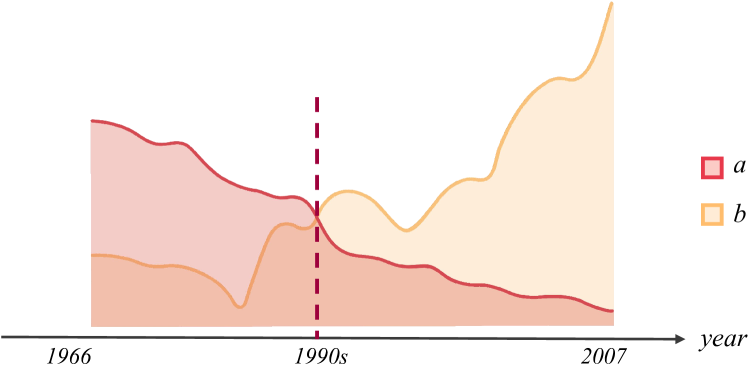
Figure 1. Jim Gray’s Activeness in database community (a) and astronomy (b) community.

However, merely counting butterflies across the entire timeline, as suggested by (Cai et al., 2024), may not accurately reflect the dynamic nature of relationships, failing to capture evolving trends. For example, in academics, a known scientist may change frequent collaborators and research interests over time. She/he might shift her/his research interest and community over time. Consequently, an aggregate count of butterflies across all publications and collaborations might not accurately represent the scientist’s research focus or capability during specific periods. To address this, it is essential to consider the temporal dimension of interactions. By focusing on the occurrence of motifs within specified time frames, we introduce the concept of historical butterfly counting. This approach, which involves analyzing butterflies within discrete time windows on a temporal bipartite graph, offers enhanced insights into the timing and progression of interactions. It provides an in-depth understanding of network dynamics, uncovering the mechanisms behind network evolution and revealing opportunities for precise interventions across various domains. For instance, examining two series of two-year historical bipartite clustering coefficients (derived from historical butterfly counts) within the research domains of Jim Gray in Figure 1, specifically the database and astronomy communities, reveals a gradual shift in his research interests from databases to astronomy around the 1990s.

Counting butterflies in such a historical setting is challenging. One main reason is that the algorithm should be able to answer historical queries multiple times to analyze the changing trend. When the graph is large, running previous algorithms from scratch whenever we have a query is inefficient. Thus, we need to design algorithms that support efficient multiple queries after preprocessing, which no algorithm can effectively solve this problem in existing works. This paper fills this hole by proposing a new index algorithm with consistently high performance in large-scale graphs. The proposed algorithm GSI can take advantage of graph structures and balance between query time and memory usage, enabling it to outperform previous butterfly counting algorithms in this setting on both real-world data and synthetic data with certain distributions. Our algorithm can also be parallelized, providing faster query efficiency. To summarize, we have made the following contributions to this work.

1. We introduce the novel historical butterfly counting problem and provide its hardness, enabling in-depth trend and dynamics analysis over temporal graphs and setting the stage for understanding how temporal variations influence network structures and interactions over time.

2. A graph structure-aware index (GSI) is designed to support efficient counting query evaluation with a controllable balance between query time and memory usage.

3. Theoretically, we prove that our GSI approach transcends conventional computational complexity barriers associated with general graphs when applied to power-law graphs, a common characteristic of many real-world graphs.

4. Extensive experiments demonstrate that our query algorithm achieves up to five orders of magnitude speedup over the state-of-the-art solutions with manageable memory footprints.

Overview

We discuss related work in Section 2. In Section 3, we formally introduce the historical butterfly counting problem, along with useful notations and necessary tools. The proposed index GSI is introduced and analyzed in Section 4.

In Section 5, we analyze GSI on the known power-log model. Experimental results are provided and discussed in Section 6. In Section 7, we provide a case study on the author-publication dataset, demonstrating the usage of historical butterfly counting. Section 8 concludes the paper.

2. RELATED WORK

In this section, we review the related works, including the butterfly counting on static bipartite graphs, motif counting on temporal graphs, and other historical queries on temporal graphs.

$\bullet$ Butterfly counting on static Bipartite Graphs. Butterfly is the most fundamental sub-structure in bipartite graphs. Significant research efforts have been dedicated to the study of counting and enumerating butterflies on static bipartite Graphs (Wang et al., 2019; Sanei-Mehri et al., 2018; Wang et al., 2014). Wang et al. (Wang et al., 2014) first proposed the butterfly counting problem and designed an algorithm by enumerating wedges from a randomly selected layer. Sanei-Mehri et al. (Sanei-Mehri et al., 2018) further developed a strategy for choosing the layer to obtain better performance. Recently, Wang et al. (Wang et al., 2019) utilized the vertex priority and cache optimization to achieve state-of-the-art efficiency. Additionally, the parallel algorithms (Sanei-Mehri et al., 2018; Shi and Shun, 2022), I/O efficient algorithm (Wang et al., 2023a), sampling-based algorithms (Sanei-Mehri et al., 2018; Li et al., 2021; Sheshbolouki and Özsu, 2022), GPU-based algorithm (Sheshbolouki and Özsu, 2022), and batch update algorithm (Wang et al., 2023b) have also been developed for the butterfly counting problem. In addition, the butterfly counting problems in steam, uncertain, and temporal bipartite graphs have also been studied (Cai et al., 2024; Sheshbolouki and Özsu, 2022; Sanei-Mehri et al., 2019; Zhou et al., 2021).

$\bullet$ Motif Counting on Temporal Graphs. The problem of temporal motif counting has been extensively studied recently (Boekhout et al., 2019; Gurukar et al., 2015; Li et al., 2018; Liu et al., 2021; Kovanen et al., 2011). Kovanen et al. (Kovanen et al., 2011) introduced the concept of $\Delta$-adjacency, which pertains to two temporal edges sharing a vertex and having a timestamp difference of at most $\Delta$, and consider the temporal ordering aspect. The $\delta$-temporal motif counting with (Pashanasangi and Seshadhri, 2021; Redmond and Cunningham, 2013) and without temporal ordering (Paranjape et al., 2017) are also been studied. Furthermore, there are numerous approximation algorithms available for solving counting problems (Liu et al., 2019a; Sarpe and Vandin, 2021). When it comes to enumeration problems, isomorphism-based algorithms are the most commonly used (Li et al., 2019; Locicero et al., 2021).

$\bullet$ Other historical queries on temporal graphs. The historical queries on the temporal graphs aim to compute the specific structure in the snapshot of an arbitrary time window. The historical reachability (Wen et al., 2022), $k$-core (Yu et al., 2021), structural diversity (Chen et al., [n. d.]), and connected components (Xie et al., 2023) of temporal graphs have been defined, and index-based solutions have also been proposed.

Note that our work is significantly different with (Cai et al., 2024), as our work is focused on more generalized scenarios of temporal graph mining, i.e., analyzing the relationship between vertices in a small time interval and without any temporal ordering limitations.

3. Preliminaries

3.1. Notations

Throughout the paper, we use the big-O notation to express the upper bounds of the absolute values of functions. For example, $O(\frac{1}{n})$ includes functions between $-\frac{c}{n}$ and $\frac{c}{n}$ for some constant $c$ and sufficient large $n$. We say $f(n)\geq g(n)+O(h(n))$ if $f(n)\geq g(n)-c|h(n)|$ for some constant $c$ and sufficient large $n$.

We use $[n]$ to denote the set $\{1,\ldots,n\}.$

For an undirected graph, we denote every vertex $u$’s degree as $deg_{u}$. The concept of degeneracy is vital to our algorithm analysis. The formal definition is as follows:

Definition 3.1 (Degeneracy).

Given an undirected graph $G=(V,E)$, its degeneracy $\delta(G)$ is denoted as $\frac{1}{m}\sum_{(u,v)\in E}\min(deg_{u},deg_{v})$.

3.2. Problem Definitions

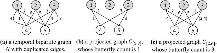
Figure 2. A temporal bipartite graph and its projected graphs in two time-windows, associated with their butterfly counts.

On bipartite graphs, there are two common motifs being widely studied: wedges and butterflies. We give their formal definition as follows:

Definition 3.2 (Wedge (Wang et al., 2019)).

Given a bipartite graph $G=(V=(U,L),E)$, a wedge $\left\langle x\leadsto y\leadsto z\right\rangle$ is a 2-hop path consisting of edges $(x,y)$ and $(y,z)$.

Definition 3.3 (Butterfly (Wang et al., 2019)).

Given a bipartite graph $G=(V=(U,L),E)$, and the four vertices $x,y,z,w\in V$ where $x,z\in U$ and $y,w\in L$, $b:\left\langle x,y,z,w\right\rangle$ is a butterfly iff the subgraph induced by $x,y,z,w$ is a $(2,2)$-biclique of $G$; that is, $x$ and $z$ are all connected to $y$ and $w$, respectively.

Throughout the paper, we study the temporal bipartite graphs. A temporal bipartite graph is an undirected graph $G=(V=(U,L),E)$, where each edge $e\in E$ is a triple $(u,v,t)$ with two vertices $u\in U,v\in L$ and a timestamp $t$. Our major focus is the historical type query on temporal bipartite graphs; that is, we query on an extracted graph from $G$ with respect to a certain time window. We denote it as the projected graph and its formal definition is as follows:

Definition 3.4 (Projected graph (Fang et al., 2020)).

Given a temporal bipartite graph $G=(V,E)$ and a time-window $[t_{s},t_{e}](t_{s}\leq t_{e})$, the projected graph $G_{[t_{s},t_{e}]}$ of $G$ is an undirected bipartite graph without timestamps, where its vertex set $V_{[t_{s},t_{e}]}$ is $V$ and the edge set $E_{[t_{s},t_{e}]}$ is $\{(u,v)\ |\ \exists(u,v,t)\in E\ \land\ t\in[t_{s},t_{e}]\}$.

Now, we are ready to state the major problem formally:

Problem 1 (Historical butterfly counting).

Given a temporal bipartite graph $G$ and a time-window $[t_{s},t_{e}]$, find the number of butterflies in the projected graph $G_{[t_{s},t_{e}]}$.

In Figure 2, we are given a temporal bipartite graph $G$ in (a), in which the number represents the timestamp of each edge. We consider two time-windows $[1,3]$ and $[2,6]$. The corresponding projected graphs $G_{[1,3]}$ and $G_{[2,6]}$ are shown in (b) and (c), respectively. The historical butterfly counting query associated with these two-time windows is, in fact, counting on these two projected graphs. Therefore, the answer is $1$ ($\left\langle 1,3,4,5\right\rangle$) for $[1,3]$ and $3$ ($\left\langle 1,2,4,5\right\rangle$, $\left\langle 1,3,4,5\right\rangle$, $\left\langle 2,3,4,5\right\rangle$) for $[2,6]$.

3.3. Tools

Our proposed algorithms widely use two important techniques: the Vertex Priority method and the Chazelle’s structure.

Vertex Priority

The vertex priority method reduces the number of wedges we need to consider. To begin with, we define the vertex priority as follows:

Definition 3.5 (Vertex priority (Wang et al., 2019)).

For any pair vertices $x,y$ in a temporal bipartite graph $G$, we define $x$ is prior to $y$ ($pr(x)\prec pr(y)$) if and only if:

• $\overline{deg}_{x}$ ¿ $\overline{deg}_{y}$, or

• $\overline{deg}_{x}$ = $\overline{deg}_{y}$ and $id(x)<id(y)$,

where $\overline{deg}_{u}$ denotes the degree of $u$ when only considering unique edges in $G$, and $id(u)$ denotes the unique ID of $u$.

By  (Wang et al., 2019), we only need to consider the wedges $\left\langle x\leadsto y\leadsto z\right\rangle$ that satisfy $pr(x)\prec pr(y)\land pr(x)\prec pr(z)$ in order to count the butterflies without repetition or missing. Each butterfly $\left\langle x,y,z,w\right\rangle$ is constructed from two such wedges $\left\langle x\leadsto y\leadsto z\right\rangle$ and $\left\langle x\leadsto w\leadsto z\right\rangle.$

2D-range Counting

Our algorithm will transform counting butterflies into counting points on a 2-dimensional plane, known as the 2D-range counting problem. Specifically, let $P$ be a set of $n$ points in 2-d space $\mathbb{R}^{2}$. The 2D-range counting problem is: Given an orthogonal rectangle $Q$ of the form $[x_{1},x_{2}]\times[y_{1},y_{2}]$, find the size of $|Q\cap P|$.

For an instance of the 2D-range counting problem, we use a classic data structure known as Chazelle’s structure (Chazelle, 1988) to handle all 2D-range counting queries after preprocessing:

Theorem 3.1 (Chazelle’s structure (Chazelle, 1988)).

A Chazelle’s structure $\mathcal{CS}$ is a data structure that can answer each 2D-range counting in $O(\log n)$ time and $O(\frac{n\log n}{\omega})$ memory usage, where $\omega$ is the word size. The preprocessing time is $O(n\log n)$.

In practice, $2^{\omega}$ significantly exceeds the number of points involved in our method’s 2D-range counting task. Therefore, we assume that $\log n$ is $O(\omega)$ for Chazelle’s structures used and simplify the memory usage into $O(n)$ for brevity. In later sections, we use $\mathcal{CS}$ to denote such a data structure.

3.4. Baselines

We compare our methods against the states-of-the-arts online methods for exact butterfly counting (i.e., BFC-VP++ (Wang et al., 2019)) and approximate butterfly counting (i.e., Weighted Pair Sampling (WPS) (Zhang et al., 2023)).

• BFC-VP++: The BFC-VP++ algorithm sorts vertices by their proposed vertex priority (3.5) and efficiently identifies almost all minimally redundant wedges that can form a butterfly, offering a practical, efficient, and cache-friendly solution. In addition, BFC-VP++ can be highly parallelized. We will also compare our methods with its parallel version in the following.

• WPS: The basic idea behind WPS is to estimate the total butterfly count with the number of butterflies containing two randomly sampled vertices from the same side of the two vertex sets. The method has been proven as unbiased and theoretically efficient in power-law graph models.

4. INDEX-BASED ALGORITHMS

In this section, we consider solving 1 exactly by index-based solutions. To begin with, in Section 4.1, we give a hardness result showing that $\widetilde{O}(m^{2}/\lambda^{2})$ space is needed to answer queries exactly in $\widetilde{O}(\lambda)$ time, where $m$ denotes the number of edges in the given temporal bipartite graph $G$. Correspondingly, we provide an algorithm that meets such bound in Section 4.2, named as Enumeration-based Index (EBI). EBI achieves $\widetilde{O}(1)$ query time but it needs expensive memory usage for large graph data. In Section 4.3, we introduce a different algorithm named Combination-based Index (CBI) that can be constructed under practical memory constraints.

To bridge the gap between theory and practice, we propose a new algorithm in Section 4.4 that effectively combines EBI and CBI, demonstrating strong performance on real-world graph data. This algorithm, named Graph Structure-aware Index (GSI), intelligently allocates graph data to the two indices which allows it to take advantage of the underlying graph structure. In addition, without compromising the performance, GSI can also handle duplicate edges with proper modification. We discuss the technical details in Section 4.5.

4.1. Problem Hardness

Our result is motivated by the hardness result in (Deng et al., 2023) where they reduce the Set Disjointness problem (4.1) into 1. While (Deng et al., 2023) considers timestamps on vertices, we construct a separate hardness proof for the setting where timestamps are on edges.

Definition 4.1 (Set Disjointness).

Given a collection of $s\geq 2$ sets $S_{1}$, $S_{2}$, $\ldots$,$S_{s}$, a query $(a,b)\in[s]^{2}$ asks for whether $S_{a}\cap S_{b}$ is empty.

The strong set disjointness conjecture (Goldstein et al., 2017, 2019) is as follows:

Theorem 4.1.

For the set disjointness problem, any data structure with query time $\lambda$ must use $\widetilde{\Omega}(n^{2}/\lambda^{2})$ space where $n$ is the sum of the sizes of $S_{1},\ldots,S_{s}$.

Specifically, we prove the following result for 1:

Theorem 4.2.

Consider 1. Let $m$ denote the number of edges in $G$. Fix any $\lambda\in[1,m]$ and $\delta>0$. Suppose that we have a data structure for 1 using $\widetilde{O}(m^{2-\delta}/\lambda^{2})$ space and exactly answers each query in $\widetilde{O}(\lambda)$ time. Then, for any set disjointness problem with $\sum_{i=1}^{s}|S_{s}|=N$, we have a data structure that uses $\widetilde{O}(N^{2-\delta}/\lambda^{2})$ time and that +answers each query in $\widetilde{O}(\lambda)$ time.

Proof.

Suppose that we have a data structure for 1 using $\widetilde{O}(m^{2-\delta}/\lambda^{2})$ space and exactly answers each query in $\widetilde{O}(\lambda)$ time. We can utilize the data structure for a set disjointness instance as follows:

Let there be $s$ sets $S_{1},\ldots,S_{s}$. Without loss of generality, we let $1,\ldots,t$ denote all distinct elements in $S_{1},\ldots,S_{s}$, i.e., $\bigcup_{i=1}^{s}S_{i}=[t]$. We construct a graph $G=(V=(U,L),E)$ such that $U=[s]$ and $L=[t+1]$. An edge $(i,j)$ exists if $j\in S_{i}$ or $j=t+1$. We assign timestamp $i$ to the edge $(i,j)$.

We build the data structure for the graph $G$ defined above. For two integers $a\leq b\in[s]$, we can query the data structure for the number of butterflies in the time window $[a,b]$. Since the timestamp on edge $(i,j)$ is equal to $i$, such butterflies are exactly those with the form $\left<u,v,w,x\right>$ such that $u,w\in[a,b]$. The number of such butterflies is

$$Q(a,b)\overset{\text{\tiny def}}{=}\sum_{i=a}^{b}\sum_{j=i+1}^{b}\left(\begin{array}[]{c}|S_{i}\cap S_{j}|+1\\ 2\end{array}\right).$$

Notice that $Q(a,b)$ is the two-dimensional prefix sum of $\binom{|S_{a}\cap S_{b}|+1}{2}$. In other words, we can calculate $\binom{|S_{a}\cap S_{b}|+1}{2}$ by $Q(a,b)-Q(a+1,b)-Q(a,b-1)+Q(a+1,b-1)$, where we define $Q(x,y)=0$ for $x\geq y$. We can answer whether $|S_{a}\cap S_{b}|=0$ by checking whether this value is equal to zero.

∎

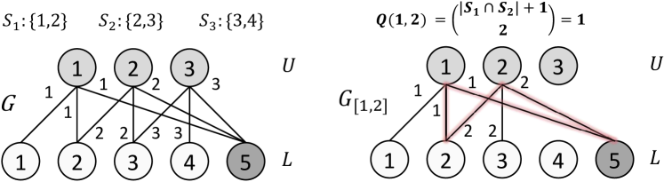
Figure 3. An example for reducing the set disjointness problem into exact historical butterfly counting in temporal bipartite graphs.

For example, in the Figure 3, we reduce the set disjointness problem for three sets $\{1,2\}$, $\{2,3\}$ and $\{3,4\}$ to a historical butterfly counting problem on the graph we constructed. For determining whether $S_{1}\cap S_{2}$ is empty, we count the number of butterflies of the form $\left<1,v,2,x\right>$, $Q(1,2),$ which is equal to $\binom{\left|S_{1}\cap S_{2}\right|+1}{2}$. For determining whether $S_{1}\cap S_{3}$ is empty, we calculate $\binom{|S_{1}\cap S_{3}|+1}{2}=Q(1,3)-Q(2.3)-Q(1,2)+Q(2,2)=2-1-1+0=0$.

This hardness result shows that to achieve efficient query runtime (e.g., $\widetilde{O}(\lambda)$), large memory space is necessary (e.g., $\widetilde{O}(m^{2}/\lambda^{2})$). Even though we can design theoretically optimal algorithms that reach the lower bound, they might not be practical when the input graph is large. One possible way to overcome such a challenge from a practical perspective is to develop algorithms that take advantage of real-world graphs’ properties.

4.2. Enumeration-based Index

Since the structure of a temporal graph changes over time, each subgraph has its own life cycle, i.e., the only interval of time in which it exists. We denote such an interval as the active timestamp of this subgraph. We give a formal definition as follows:

Definition 4.2 (Active Timestamp).

For any subgraph $P$ of a bipartite temporal graph $G$, we define the active timestamp $\mathcal{T}(P)$ as a pair of ordered timestamp $[l,r](l\leq r)$, such that $P$ exist in the projected graph $G_{[t_{s},t_{e}]}$ if and only if $t_{s}\leq l$ and $r\leq t_{e}$.

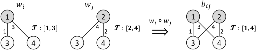
Figure 4. An illustrative example for active timestamps of wedges and the butterfly constructed from them.

In Figure 4, there are two wedges $w_{i}$ and $w_{j}$. For $w_{i}$, since it contains two edges $(1,3,1)$ and $(1,4,3)$, it only exists in a projected graph $G_{[t_{s},t_{e}]}$ satisfying $t_{s}\leq 1$ and $t_{e}\geq 3$. The active timestamp $\mathcal{T}(w_{i})$ is $[1,3]$. Similarly, for $w_{j}$, its active timestamp is $[2,4]$.

The proposed Enumeration-based Index (EBI) algorithm is shown in Algorithm 1 and Algorithm 2. For brevity, we assume that no duplicate edge exists. We will discuss how to handle duplicate edges without compromising the performance in Section 4.5.

Construction

The goal is to enumerate every butterfly and compute its active timestamp. After initializing a 2D-range counting data structure $T_{E}$ by all butterflies’ timestamps, we can answer every historical butterfly counting query through a single query on $T_{E}$. We initialize it to be empty in the beginning (Algorithm 1).

To find all the butterflies in $G$, we enumerate all the wedges. We consider two wedges $w_{i},w_{j}$ of $G$ with shared endpoints but different middle vertices, denoted as $w_{i}:\left\langle x\leadsto y_{i}\leadsto z\right\rangle$ and $w_{j}:\left\langle x\leadsto y_{j}\leadsto z\right\rangle$. Let $\mathcal{T}(w_{i})=[l_{i},r_{i}]$ and $\mathcal{T}(w_{j})=[l_{j},r_{j}]$. The temporal butterfly constructed from them is denoted as $b_{ij}=w_{i}\circ w_{j}$, where $\mathcal{T}(b_{ij})=[\min(l_{i},l_{j}),\max(r_{i},r_{j})]$.

In Figure 4, we demonstrate how to construct a butterfly $b_{ij}$ with two wedges $w_{i}$ and $w_{j}$. Since $b_{ij}$ contains edges $(1,3,1)$, $(1,4,3)$, $(2,3,4)$, and $(2,4,2)$, its active timestamp can be computed by $l=\min\{t|\ \exists e=(u,v,t)\in edges(b_{ij})\}=1,$ and $r=\max\{t|\ \exists e=(u,v,t)\in b_{ij}\}=4$. By the definition of the $\circ$ operation, it can also be computed from $\mathcal{T}(w_{i})$ and $\mathcal{T}(w_{j})$. This also indicates that a butterfly $b_{ij}=w_{j}\circ w_{j}$ exists in a given time-window, if and only if the active timestamp of $w_{i}$ and $w_{j}$ are both included in the window. Such observation helps us develop an alternative index approach in the later section.

We follow the method in (Wang et al., 2019) to enumerate every wedge $w_{i}:\left\langle x\leadsto y\leadsto z\right\rangle[l_{i},r_{i}]$ in $G$ without repetition or missing (Algorithm 1). The complexity is bounded by the total number of wedges in $G$. Let $W[(x,z)]$ be a set of wedges whose endpoints are $x,z$. $W$ is the family of sets $W[(x,z)]$. $W$ is initialized to be empty in the beginning (Algorithm 1). For the current wedge $w_{i}$, we first check if its endpoints $(x,z)$ exists in $W$ (Algorithm 1) (by a hash table, for example). If not, we initialize the corresponding set $W[(x,z)]$ to be empty (Algorithm 1).

Since any two different wedges with the same pair of endpoints $(x,z)$ construct a unique butterfly, we enumerate every $w_{j}$ in
$W[(x,z)]$ (Algorithm 1) and construct a butterfly $b_{ij}=w_{i}\circ w_{j}$ with $\mathcal{T}(b_{ij})=(t_{l},t_{r})$ (Algorithm 1). Correspondingly, we insert a single 2D point $(t_{l},t_{r})$ into $T_{E}$. After enumeration, we need to update $W[(x,z)]$ by inserting $w_{i}$ in it (Algorithm 1). After finding all the butterflies, we run the preprocessing for $T_{E}$ and return it (Algorithm 1).

In Figure 5, we provide an example of our construction process. There are three wedges $w_{1}:\left\langle 1\leadsto 4\leadsto 2\right\rangle$, $w_{2}:\left\langle 1\leadsto 5\leadsto 2\right\rangle$, $w_{3}:\left\langle 1\leadsto 4\leadsto 3\right\rangle$, $w_{4}:\left\langle 1\leadsto 5\leadsto 3\right\rangle$, $w_{5}:\left\langle 2\leadsto 4\leadsto 3\right\rangle$, $w_{6}:\left\langle 2\leadsto 5\leadsto 3\right\rangle$ where $\mathcal{T}(w_{1})=[4,6]$, $\mathcal{T}(w_{2})=[2,5]$, $\mathcal{T}(w_{3})=[4,4]$, $\mathcal{T}(w_{4})=[2,4]$, $\mathcal{T}(w_{5})=[4,6]$, $\mathcal{T}(w_{6})=[4,5]$. We group them by $(x,z)$. There will be three groups (sets) of wedges: $W[(1,2)]=\{w_{1},w_{2}\}$, $W[(1,3)]=\{w_{3},w_{4}\}$, $W[(2,3)]=\{w_{5},w_{6}\}$. For each group, we construct a butterfly $b_{ij}$ from each pair of different wedges $w_{i},w_{j}$ from the group. We have $b_{1}=w_{1}\circ w_{2}$, $b_{2}=w_{3}\circ w_{4}$, $b_{3}=w_{5}\circ w_{6}$. We compute their active timestamp through simple calculation: $\mathcal{T}(b_{1})=[2,4]$, $\mathcal{T}(b_{2})=[2,6]$, $\mathcal{T}(b_{3})=[4,6]$. In the end, we insert $(2,4)$, $(2,6)$, $(4,6)$ into $T_{E}$. Note that in this showcase, for demonstrating the group dividing, we do not follow the vertex priority in 3.5. Otherwise, we only consider three wedges and they are all in the group $W[(4,5)]$.

Answering Query

Since each butterfly with active timestamp $[l,r]$ is represented by a point $(l,r)$ in $T_{E}$, a historical butterfly counting of time-window $[t_{s},t_{e}]$ can be interpreted as a 2D-range query counting the number of points in the rectangle $[t_{s},\infty]\times[-\infty,t_{e}]$. We query $T_{E}$ for it and return the answer directly (Algorithm 2).

In Figure 5, after the preprocessing of $T_{E}$, we can answer any 2D-range counting query concerning those three points, which represent the three butterflies. When we want to query the number of butterflies in time-window $[1,5]$, we are asking how many butterflies’ active timestamps are in the range of $[1,5]$. We interpret this as querying the number of points in the rectangle $[1,\infty]\times[-\infty,5]$. There is only one point $(2,4)$ in the rectangle. Therefore, there is only one butterfly in the projected graph of the queried time-window. The calculation is done by a single query on $T_{E}$. It is a typical 2D-range counting query.

Time and Space Complexity

The time and space complexity of EBI is summarized as follows:

Theorem 4.3.

Denote $B$ as the number of butterflies and $\delta$ as the degeneracy of the input graph $G$. EBI’s construction (Algorithm 1) runs in $O(m\delta+B\log m)$ and takes $O(B)$ space. After the construction, each query (Algorithm 2) takes $O(\log m)$ to answer.

Proof.

The construction process requires enumerating all wedges. By (Wang et al., 2019), this takes $O(m\delta)$. For each wedge $w_{i}:\left\langle x\leadsto y\leadsto z\right\rangle$, it is inserted in $W[(x,z)]$. By enumerating every existing $w_{j}$ in $W[(x,z)]$, every butterfly $b_{ij}=w_{i}\circ w_{j}$ is enumerated exactly once. Since the $\circ$ operation takes $O(1)$ and the insertion to $T_{E}$ takes $O(\log m)$ by Theorem 3.1, the total preprocess time for all butterflies takes $O(B\log m)$. Therefore, the total runtime for Algorithm 1 is $O(m\delta+B\log m)$ as desired. Every wedge will be stored in $W[(x,z)]$ where $x,z$ are its endpoints. All the wedges take $O(m\delta)$ space in total. $T_{E}$ contains $O(B)$ points in total. By Theorem 3.1, it takes $O(B)$ space. The total memory usage sum up to $O(B+m\delta)$. Each query on EBI is a range query on $T_{E}$. By Theorem 3.1, this takes $O(\log m)$ time and no additional space. ∎

The EBI algorithm reaches the bound mentioned in Section 4.1: Since $\delta$ is bounded by $O(\sqrt{m})$ and $B$ is bounded by $O(m^{2})$, the memory usage is bounded by $\widetilde{O}(m^{2})$. Therefore, EBI answers each query in $\widetilde{O}(1)$ time and take $\widetilde{O}(m^{2})$ space. This indicates that EBI’s asymptotic memory usage cannot be further improved without affecting the $\widetilde{O}(1)$ query time. On the other hand, though reaching theoretical optimality, EBI’s performance on large-scale data is not ideal because enumerating and storing all butterflies are challenging for these graphs. For example, in the Wiktionary dataset, the butterfly count exceeds $10^{16}$ where the graph contains about $4\times 10^{7}$ edges.

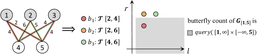
Figure 5. An example for transforming historical butterfly counting into 2D-range counting.

Input: a bipartite temporal graph: $G=(V,E)$;

Output: a $\mathcal{CS}$ (Theorem 3.1) for indexing (EB-index): $T_{E}$;

1 Initialize $T_{E}$ with an empty $\mathcal{CS}$;

2 $W\leftarrow$ an empty hashmap mapping pairs of vertices to sets;

3 for each wedge $w_{i}:\left\langle x\leadsto y\leadsto z\right\rangle[l_{i},r_{i}]\in G$ do

4       if $(x,z)\notin W.keys()$ then  $W[(x,z)]\leftarrow\emptyset$ ;

5       for $w_{j}\in W[(x,z)]$ do

6             $b_{ij}\leftarrow w_{i}\circ w_{j}$;

             $T_{E}.insert(t_{l},t_{r})$;

              // $(t_{l},t_{r})=\mathcal{T}(b_{ij})$

7            

8      $W[(x,z)]\leftarrow W[(x,z)]\cup w_{i}$;

9Preprocess $T_{E}$ (Theorem 3.1);

return $T_{E}$;

Algorithm 1 EBI-Construction

Input: a time-window: $[t_{s},t_{e}]$; a EB-index: $T_{E}$;

Output: temporal butterfly counting: $num_{[t_{s},t_{e}]}$;

return $num_{[t_{s},t_{e}]}\leftarrow T_{E}.query([t_{s},\infty]\times[-\infty,t_{e}])$;

Algorithm 2 EBI-Querying

4.3. Combination-based Index

If the graph is large, it is not realistic to pre-compute and store all butterflies to handle historical queries, as this requires too much space. On the other hand, we are only interested in the number of butterflies, so it is not necessary to construct them explicitly.

Recall that a butterfly exists in a given time window if and only if the active timestamp of the two wedges are both included in the window. Consider a group of wedges $S=\{\left\langle x\leadsto y\leadsto z\right\rangle\}$ where $x,z$ are fixed. Any two wedges from $S$ form a butterfly. Therefore, the total number of butterflies that comes from $S$ is $\binom{|S|}{2}$. This idea leads us to a different index algorithm, named Combination-based Index (CBI). The implementation details are provided in Algorithm 3 and Algorithm 4. Similarly, we assume no duplicate edge for brevity. Resolving them is deferred to Section 4.5.

Construction

In EBI, we use one 2D-counting data structure to store butterflies. Instead, in CBI, we map every type of wedge to a separate data structure. We initialize a hashmap $T_{C}$ in the beginning (Algorithm 3). We still need to enumerate every wedge $w_{i}:\left\langle x\leadsto y\leadsto z\right\rangle[l_{i},r_{i}]$ in $G$ (Algorithm 3). A wedge with endpoints $x,z$ is maintained by the 2D-counting data structure $T_{C}[(x,z)]$. If $T_{C}[(x,z)]$ does not exist(Algorithm 3), we initialize an empty $\mathcal{CS}$ ((Theorem 3.1) for $T_{C}[(x,z)]$ (Algorithm 3). Unlike in EBI, where we compute every butterfly that is constructed from the new wedges $w_{i}$ and a previous wedge $w_{j}\in W[(x,z)]$, we directly insert a point $[l_{i},r_{i}]$ ($w_{i}$’s active timestamp) into the corresponding $T_{C}[(x,z)]$ (Algorithm 3). After the enumeration, we preprocess all data structures $T_{C}[(x,z)]$ and return $T_{C}$ (Algorithm 3).

Answering Query

To answer a historical butterfly counting of time-window $[t_{s},t_{e}]$, for every type of wedges, we first need to compute the number of wedges that exist in the time-window, then compute the number of butterflies by a simple binomial coefficient. We set a counter $num_{[t_{s},t_{e}]}$ to be $0$ initially (Algorithm 4). We enumerate every existing data structure in $T_{C}$ (Algorithm 4). Similar to what we do in EBI, we query on the corresponding 2D-counting data structure $T_{C}[(x,z)]$ with a query $[t_{s},\infty]\times[-\infty,t_{e}]$ to get the number of wedges that are active in the time-window (Algorithm 4). Denoting the query answer as $count$, we add $\binom{count}{2}$ to $num_{[t_{s},t_{e}]}$, which is the number of butterflies that are constructed from these wedges. After enumerating all the data structures, we return $num_{[t_{s},t_{e}]}$ as the total number of butterflies (Algorithm 3).

Time and Space Complexity

The time and space complexity of CBI is summarized as follows:

Theorem 4.4.

Denote $\widetilde{w}$ as the number of wedge groups and $\delta$ as the degeneracy of the input graph $G$. CBI’s construction (Algorithm 3) runs in $O(m\delta\log n)$ and takes $O(m\delta)$ space. After the construction, CBI answers each query (Algorithm 4) in $O(\widetilde{w}\log n)$ time.

Proof.

The construction process (Algorithm 3) also requires enumerating all wedges, which takes $O(m\delta)$ by (Wang et al., 2019). For each group of wedges with the same endpoints, a $\mathcal{CS}$ will need to be initialized with all wedges from this group. Since the number of wedges is bounded by $O(m\delta)$ and each group contains at most $O(n)$ wedges, the total time for preprocessing all the data structures is $O(m\delta\log n)$ by Theorem 3.1. Similar to Theorem 4.3, it takes $O(m\delta)$ memory in total. When answering a query (Algorithm 4), all groups of wedges need to be enumerated, and their corresponding $\mathcal{CS}$ will be queried exactly once. The total query time will be $O(\widetilde{w}\log n)=\widetilde{w}\times O(\log n)$ by Theorem 3.1. The memory usage is dominated by 2D-range counting data structures of each group of wedges. ∎

As a result, CBI manages to resolve the memory issue of EBI when there are too many butterflies. Although $\widetilde{w}$ is bounded by the number of wedges (i.e., $m\delta$), in practice, it is significantly smaller (i.e., $\widetilde{w}\ll m\delta$). For example, in the Wiktionary dataset, there is about $m\delta\approx 1.3\times 10^{9}$ wedges but only $\widetilde{w}\approx 5\times 10^{7}$ wedge groups with different $(x,z)$.

By further observing the distribution of wedges on real-world data, we see a concentration phenomenon that our algorithm has not addressed: Most wedges are grouped in a few groups, while the rest contain only a very small number of wedges. Therefore, building a separate data structure for every wedge group might be too expensive and unnecessary, especially for groups that only contribute a small amount of butterflies. For example, in the Wiktionary (WT) dataset, more than $81.3$% wedge groups contain less than 10 wedges.

Input: a bipartite temporal graph: $G=(V,E)$;

Output: a hashmap mapping pairs of vertices to multiple $\mathcal{CS}$s: $T_{C}$;

1

2$T_{C}\leftarrow$ an empty hashmap mapping pairs of vertices to $\mathcal{CS}$s;

3 for each wedge $w_{i}:\left\langle x\leadsto y\leadsto z\right\rangle[l_{i},r_{i}]\in G$ do

4       if $(x,z)\notin T_{C}.keys()$ then

5             Initialize $T_{C}[(x,z)]$ with an empty $\mathcal{CS}$;

6      $T_{C}[(x,z)].insert(l_{i},r_{i})$;

7      

8Preprocess each data structure in $T_{C}$ (Theorem 3.1);

return $T_{C}$;

Algorithm 3 CBI-Construction

Input: a time-window: $[t_{s},t_{e}]$; a CB-index: $T_{C}$;

Output: temporal butterfly counting: $num_{[t_{s},t_{e}]}$;

1 $num_{[t_{s},t_{e}]}\leftarrow 0$;

2 for $(x,z)\in T_{C}.keys()$ do

3       $count\leftarrow T_{C}[(x,z)].query([t_{s},\infty]\times[-\infty,t_{e}])$;

4       $num_{[t_{s},t_{e}]}\leftarrow num_{[t_{s},t_{e}]}+\binom{count}{2}$

return $num_{[t_{s},t_{e}]}$;

Algorithm 4 CBI-Querying

4.4. Graph Structure-aware Index

Recall that the number of butterflies dominates the memory usage of EBI, and the number of wedge groups greatly affects the query time of CBI. They fail to take into account the actual structure of the input graph. If we assume that most wedge groups only contain a very small amount of wedges, we might be able to take advantage of both EBI and CBI by distributing each wedge group into one of EBI and CBI by its size. As the main result of our paper, we propose a new index algorithm named Graph Structure-aware Index (GSI) with such an idea. Besides its promising performance on real-world data, it can also be parallelized to reach an even better performance. The implementation details are provided in Algorithm 5 and Algorithm 6.

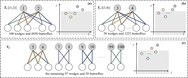
Figure 6. An illustrative example for demonstrating GSI.

Construction

The important assumption we make here is that a small number of groups contain most of the wedges. Our key idea is to store them in the same way as CBI, building a 2D-range counting data structure for each index, maintained by a hashmap $T_{C}$. For the rest of the wedges, we precompute all butterflies constructed from them and store them in one data structure $T_{E}$ like EBI. In the beginning, in addition to $T_{E}$ (Algorithm 5) and $T_{C}$ (Algorithm 5), we also initialize a hashmap $W$ to group wedges directly (Algorithm 5). We enumerate all $w_{i}:\left\langle x\leadsto y\leadsto z\right\rangle[l_{i},r_{i}]$ in $G$ (Algorithm 5) and store them into the corresponding set mapped by $W[(x,z)]$ (Algorithm 5) . If the key does not exist in $W$, we need to initialize the set to be empty (Algorithm 5). After grouping wedges, we sort the sets in $W$ with decreasing order of sizes. We also need to compute the total number of butterflies and store it in $num$ and $numB$ (Algorithm 5 to Algorithm 5).

We introduce a parameter $\alpha$ to control the cutoff between the two methods. More specifically, we will build a data structure for some sets in $W$ such that the total number of butterflies constructed from them does not exceed $\alpha$ fraction of all the butterflies in $G$. The butterflies constructed from the other sets in $W$ are maintained by one data structure per set.

We enumerate the sets in $W$ by decreasing order of sizes (Algorithm 5). $num$ represents the number of butterflies we processed. If we have not processed the majority of butterflies, i.e., when $num$ is no less than $\alpha\cdot numB$ (Algorithm 5), we build a $\mathcal{CS}$ for every wedge in $W[(x,z)]$, inserting points representing their active timestamps (Algorithm 5 to Algorithm 5). $num$ will be subtracted by $\binom{|W[(x,z)]|}{2}$, indicating that these of butterflies are recorded by $T_{C}[(x,z)]$ (Algorithm 5).

When $num$ is smaller than $\alpha\cdot numB$, we have already handled the majority of butterflies. Now, we need to process butterflies built from the rest of the wedges groups. Though each of these groups only contains a relatively small amount of wedges, the number of groups might be large. Here we apply the idea of EBI. We enumerate every possible wedge pair in the current enumerated $W[(x,z)]$ (Algorithm 5 to Algorithm 5), compute the butterfly $b_{ij}[t_{l},t_{r}]\leftarrow w_{i}\circ w_{j}$ (Algorithm 5) and insert a point $(t_{l},t_{r})$ into the global data structure $T_{E}$ (Algorithm 5). In the end, after preprocessing every $\mathcal{CS}$ in $T_{C}$ and $T_{E}$, we return them and finish the construction (Algorithm 5).

An example of construction is shown in Figure 6. In the input graph, there are 100 wedges with endpoints $(1,2)$ and 50 wedges with endpoints $(3,4)$, while there are only 97 wedges in other groups. We treat these two groups with the CBI method and build $T_{C}[(1,2)]$ (a), $T_{C}[(3,4)]$ (b) correspondingly. We compute all 50 butterflies for the remaining wedges and store them in $T_{E}$ (c).

Answering Query

For a historical butterfly counting of time-window $[t_{s},t_{e}]$, we need to accumulate answers from both $T_{C}$ and $T_{E}$. As in EBI, we directly query the 2D range $[t_{s},\infty]\times[-\infty,t_{e}]$ on $T_{E}$ (Algorithm 6). Then, as in CBI, we enumerate all groups of wedges from $T_{C}$ (Algorithm 6). We query $T_{C}[(x,z)]$ with the same 2D range (Algorithm 6) and add up the number of butterflies constructed from each group of wedges (Algorithm 6). We return the answer as the sum of these two parts (Algorithm 6). In the fig. 6 showcase, we query from all three $\mathcal{CS}$s: $T_{C}[(1,2)]$, $T_{C}[(3,4)]$, $T_{E}$ and sum up the answer.

Input: a bipartite temporal graph: $G=(V,E)$; a parameter for space using: $\alpha$;

Output: a $\mathcal{CS}$ for indexing (EB-index): $T_{E}$; a hashmap of $\mathcal{CS}$ for indexing: $T_{C}$;

1

2Initialize $T_{E}$ with an empty $\mathcal{CS}$;

3 $T_{C}\leftarrow$ an empty hashmap mapping pairs of vertices to $\mathcal{CS}$s;

4 $W\leftarrow$ an empty hashmap mapping pairs of vertices to sets;

5 for each wedge $w_{i}:\left\langle x\leadsto y\leadsto z\right\rangle[l_{i},r_{i}]\in G$ do

6       if $(x,z)\notin W.keys()$ then  $W[(x,z)]\leftarrow\emptyset$ ;

7       $W[(x,z)]\leftarrow W[(x,z)]\cup w_{i}$;

8      

9Sort sets in $W$ with decreasing order of sizes;

10 $num\leftarrow 0$;

11 for $(x,z)\in W.keys()$ do  $num\leftarrow num+\binom{|W[(x,z)]|}{2}$ ;

12 $numB\leftarrow num$;

13 for $(x,z)\in W.keys()$ do

14       if $num\geq\alpha\cdot numB$ then

15             Initialize $T_{C}[(x,z)]$ with an empty $\mathcal{CS}$;

16             for $w_{i}:[l_{i},r_{i}]\in W[(x,z)]$ do

17                   $T_{C}[(x,z)].insert(l_{i},r_{i})$;

18            

19      else

20             for $w_{i}:[l_{i},r_{i}]\in W[(x,z)]$ do

21                   for $w_{j}:[l_{j},r_{j}]\in W[(x,z)]\land(j>i)$ do

22                         $b_{ij}\leftarrow w_{i}\circ w_{j}$;

                         $T_{E}.insert(t_{l},t_{r})$;

                          // $(t_{l},t_{r})=\mathcal{T}(b_{ij})$

23                        

24                  

25            

26      $num\leftarrow num-\binom{|W[(x,z)]|}{2}$;

27      

28Preprocess $T_{E}$ and each data structure in $T_{C}$ (Theorem 3.1);

return $T_{E},T_{C}$;

Algorithm 5 GSI-Construction

Input: a time-window: $[t_{s},t_{e}]$; GSI-indexes: $T_{E},T_{C}$;

Output: temporal butterfly counting: $num_{[t_{s},t_{e}]}$;

1 $num_{[t_{s},t_{e}]}\leftarrow T_{E}.query([t_{s},\infty]\times[-\infty,t_{e}])$;

2 for $(x,z)\in T_{C}.keys()$ do

3       $count\leftarrow T_{C}[(x,z)].query([t_{s},\infty]\times[-\infty,t_{e}])$;

4       $num_{[t_{s},t_{e}]}\leftarrow num_{[t_{s},t_{e}]}+\binom{count}{2}$

return $num_{[t_{s},t_{e}]}$;

Algorithm 6 GSI-Querying

Time and Space Complexity

The time and space complexity of GSI is summarized as follows:

Theorem 4.5.

Denote $\delta$ as the degeneracy of the input graph $G$ and $\beta$ as the number of $\mathcal{CS}$ building for wedge groups. GSI’s construction (Algorithm 5) runs in $O(m\delta\log n+\alpha B\log m)$ and takes $O(m\delta+\alpha B)$ space. After the construction, each query (Algorithm 6) takes $O(\beta\log n+\log m)$ to answer.

Proof.

The construction process (Algorithm 5) requires enumerating all wedges, which takes $O(m\delta)$ by (Wang et al., 2019). The rest of the algorithm can be divided into two parts: a CBI instance of $\beta$ wedges group containing $(1-\alpha)B$ butterflies and an EBI instance containing $\alpha B$ butterflies. By Theorem 4.3 and Theorem 4.4, the total time complexity is $O(m\delta\log n+\alpha B\log m)$ and the corresponding query complexity (Algorithm 6) is $O(\beta\log n+\log m)$. The memory usage is $O(m\delta+\alpha B)$. ∎

Note that $\beta$ is determined by $\alpha$ and bounded by the number of wedge groups $\widetilde{w}$. In real-world datasets with practical memory constraints, $\beta$ is significantly smaller than $\widetilde{w}$ (i.e., $\beta\ll\widetilde{w}$). For example, in the WT dataset and under a 500 GB memory constraint, the $\beta$ of GSI is $6986$ when setting the optimal $\alpha$ that maximize the memory utilization, while the $\widetilde{w}$ is $3,925,064$.

As a result, GSI manages to address the concentration phenomenon of the wedges distribution on real-world graphs, taking advantage of both EBI (for scattered wedges) and CBI (for concentrated wedges). It also has flexibility regarding the different limitations of memory. In addition, under the well-known power-law model (Aiello et al., 2000), GSI has a non-trivial complexity. The related analysis is provided in Section 5.

4.4.1. Automatically Determining $\alpha$

The parameter $\alpha$ reflects a trade-off between query time and memory usage. Therefore, selecting a proper $\alpha$ based on the input graph and the memory limit is important. We introduce an easy method to automatically select an efficient $\alpha$ before executing GSI. In the beginning, we set $\alpha=0$, which means that all wedge groups will be maintained separately with a $\mathcal{CS}$ data structure. We sort wedge groups by size from small to large and enumerate them one by one. For each enumerated wedge group $i$ with $w_{i}$ wedges, we increase $\alpha$ by $\binom{w_{i}}{2}/B$, where $B$ is the number of butterflies, precomputed in Algorithm 5 to Algorithm 5. We can estimate the memory usage by simple calculation as Chazelle’s structure’s memory usage can be precomputed based on the number of inserted points in $O(1)$. We stop and determine $\alpha$ if the estimated memory exceeds the limit with the next wedge group. This determination process takes $O(m\delta)$ time and avoids actually building indexes.

4.4.2. Parallelized Querying

After the construction process, when answering a query (Algorithm 6), we are, in fact, summing up the answer from several independent $\mathcal{CS}$ data structures, which motivates us to utilize parallelization to speed up. Assume we have multiple threads, and these threads can handle different $\mathcal{CS}s$ simultaneously. Since no conflict occurs when these threads read the indexes simultaneously, we consider Algorithm 6 is highly parallelizable when the number of $\mathcal{CS}$s greater than the number of threads. To demonstrate, we implement and evaluate a parallel version of GSI in Section 6.2.3.

4.5. Handling Duplicate Edges

The key challenge when the graph has duplicate edges is that the life cycle of a wedge or a butterfly is no longer an active timestamp as defined in 4.2. As we will see in Appendix A, the life cycle can be decomposed into several redefined active timestamps (4.3) for graphs with duplicate edges. We will prove that the decomposition does not increase the time complexity or memory usage of GSI (Lemma 4.6 and Theorem 4.7).

Definition 4.3 (Active Intervals for Graphs with Duplicate Edges).

Given a bipartite temporal graph $G$ with duplicate edges, a subgraph $P$, we define the active intervals $\tilde{\mathcal{T}}(P)$ as a tuple of timestamps of the form $[l,r_{1},r_{2}](l\leq r_{1}\leq r_{2})$ such that $P$ is active in the query time-window $[t_{s},t_{e}]$ if and only if for exactly one of the timestamps $[l,r_{1},r_{2}]$, $t_{s}\leq l$ and $r_{1}\leq t_{e}<r_{2}$.

For applying GSI to a graph with duplicate edges, we first modify $\mathcal{CS}$ such that it can answer 2D-range queries on timestamps of the form $[l,r_{1},r_{2}],$ i.e., counting the number of $[l,r_{1},r_{2}]$ such that $t_{s}\leq l$ and $r_{1}\leq t_{e}\leq r_{2}$ given the query time-window $[t_{s},t_{e}].$ This can be done by applying the inclusive-exclusive principle on 2D ranges. Then we generate the active intervals (tuple of timestamps $[l,r_{1},r_{2}]$) for each wedge. We feed each $[l,r_{1},r_{2}]$ to GSI (with the modified $\mathcal{CS}$). A detailed explanation can be found in Appendix A.

Lastly, we prove that if the size (number of $[l,r_{1},r_{2}]$ in the tuple) of the active intervals of each wedge is bounded (Lemma 4.6), both EBI and CBI’s time complexity will not be compromised.

Lemma 4.6.

For any two vertices $u,v\in V(G)$, we denote $cnt_{u,v}$ as the number of edges $(u,v,t)\in E(G)$. There exists an algorithm (Algorithm 7 in Appendix A) that returns its active intervals (4.3) of size $O(\min(cnt_{x,y},cnt_{y,z}))$ for any wedge $\left\langle x\leadsto y\leadsto z\right\rangle$.

Proof of 4.6 can be found in Appendix A. With this lemma, we are ready to prove that the time complexity for our algorithms will not be compromised by duplicate edges:

Theorem 4.7 (Time complexity with Duplicate Edges).

(i) There exists a modification for EBI that can run in $O(\log m)$ time and $O(m^{2})$ memory usage for bipartite temporal graphs with duplicate edges; (ii) There exists a modification for CBI that can run in $O(\tilde{w}\log m)$ time and $O(m\delta)$ memory usage for bipartite temporal graphs with duplicate edges.

Proof.

(i): Considering a butterfly consisting of two wedges $\left\langle x\leadsto y_{1}\leadsto z\right\rangle$ and $\left\langle x\leadsto y_{2}\leadsto z\right\rangle$, the size of its active intervals is $O(\min(cnt_{x,y_{1}},cnt_{y_{1},z})\times\min(cnt_{x,y_{2}},cnt_{y_{2},z}))$ by Lemma 4.6. Since

$$\sum_{\text{each butterfly }\left\langle x,y_{1},z,y_{2}\right\rangle\in G}\min(cnt_{x,y_{1}},cnt_{y_{1},z})\times\min(cnt_{x,y_{2}},cnt_{y_{2},z})$$

$$\leq\sum_{\text{each butterfly }\left\langle x,y_{1},z,y_{2}\right\rangle\in G}cnt_{x,y_{1}}cnt_{y_{2},z}\leq m^{2}.$$

, the bound of the number of points in $\mathcal{CS}s$ $O(m^{2})$ for EBI still holds.

(ii): Considering a wedge $\left\langle x\leadsto y\leadsto z\right\rangle$, the the size of its active intervals in its active timestamp is $O(\min(cnt_{x,y},cnt_{y,z}))$ by Lemma 4.6. The total number of tuples for all wedges’ active timestamps is:

$$\sum_{y\in V(G)}\sum_{x\in N(y),\atop pr(x)\prec pr(y)}\sum_{z\in N(y),\atop pr(x)\prec pr(z)}\min(cnt_{x,y},cnt_{y,z})$$

$$\leq\sum_{y\in V(G)}\sum_{x\in N(y),\atop pr(x)\prec pr(y)}cnt_{x,y}deg_{x}$$

$$\leq\sum_{(x,y)\in E(G)}\min(deg_{x},deg_{y})=m\delta.$$

Therefore, the bound of the number of points in $\mathcal{CS}s$ for CBI, $O(m\delta)$, also holds. ∎

5. ANALYSIS ON POWER-LAW GRAPHS

5.1. Power-law Bipartite Graphs

Previous research (Guillaume and Latapy, 2006; Vasques Filho and O’Neale, 2018) shows that many real-world bipartite graphs follow the power-law distribution with $\gamma$ generally between $2$ to $3$, similar to the scale-free graphs model for unipartite graphs. By leveraging the properties of the power-law degree distribution, there are many studies on analyzing algorithms based on such settings (Zhang et al., 2023; Yang et al., 2021; Latapy, 2008; Brach et al., 2016). In this section, we prove that GSI runs in $\widetilde{O}(\lambda)$ time and $O(m^{2-\delta}/\lambda^{2})$ memory for some $\delta>0$ with high probability on power-law bipartite graphs (Aiello et al., 2000) with $\gamma\in(2,3)$, in contrast to the hardness result in Section 4.1 for the general case.

We use the following model for $G$.

Definition 5.1.

Let $n_{1}$ be the number of vertices in $U$. Let $n_{2}$ be the number of vertices in $L$. Let $\gamma_{i}$, $\Delta_{i}$ ($i=1,2$) be the exponents and max degrees of two power-law distributions. A power-law bipartite graph is obtained by the following process:

• For each vertex $x$ in $U$, sample $d_{x}\in[1,\Delta_{1}]$ such that

  $\mathbb{P}\left[d_{x}=k\right]\propto k^{-\gamma_{1}}$.

• For each vertex $y$ in $L$, sample $d_{y}\in[1,\Delta_{2}]$ such that

  $\mathbb{P}\left[d_{y}=k\right]\propto k^{-\gamma_{2}}$.

• Let $m=\mathbb{E}\left[\sum_{x\in U}d_{x}\right]=\mathbb{E}\left[\sum_{y\in L}d_{y}\right]$ be the expected number of edges in $G$.

• For each pair of vertices $x\in U$, $y\in L$, sample the existence of the edge $(x,y)$ such that $\mathbb{P}\left[(x,y)\text{exists}\right]=\frac{d_{x}d_{y}}{m}$.

For 5.1 to be well-defined, we need to choose parameters such that $\mathbb{E}\left[\sum_{x\in U}d_{x}\right]=\mathbb{E}\left[\sum_{y\in L}d_{y}\right]$, i.e., the expected sums of degrees for vertices in $U$ and $L$ are equal. We note that the sampled $d_{x}$ and $d_{y}$ values are intermediate variables of the sampling process. They are not necessarily the same as the degrees $\deg_{x}$ and $\deg_{y}$ of vertex $x$ and $y$. We can interpret $d_{x}$ as the expected degree of $x$.

Based on 5.1, there are two following two types of power-law bipartite graphs to model the real-world networks comprehensively.

Definition 5.2 (Double-sided Power-law Bipartite Graph).

A double-sided power-law bipartite graph is a power-law bipartite graph (5.1) satisfying $\gamma_{1}\in(2,3)$, and $\gamma_{2}\in(2,3).$

Definition 5.3 (Single-sided Power-law Bipartite Graph).

A single-sided power-law bipartite graph is a power-law bipartite graph (5.1) satisfying $\gamma_{1}\in(2,3)$, $\gamma_{2}=0,$ and $\Delta_{1}>\Delta_{2}.$

Twitter exemplifies a single-sided power-law bipartite graph, where the distribution of followers per user varies significantly, often displaying a vast disparity. In contrast, the number of accounts each user follows tends to be more uniform and comparatively narrow in range. In contrast, movie-actor networks exhibit a double-sided power-law distribution. Most actors appear in just a few films, and the majority of films feature only a small number of actors. However, a select group of highly connected actors mirrors the highly-followed users on social media platforms, while films with large casts resemble “super-connected” nodes.

5.2. Time and Space Complexity

We calculate the expected time and space complexity of GSI for each type of power-law bipartite graph.

Theorem 5.1 (GSI on double-sided power-law bipartite
graphs).

Let $G$ be a single-sided power-law bipartite graph. We can set $\alpha$ in Algorithm 5, such that the expected space usage of GSI is $O(\Delta^{6-2\gamma})$, and that the query time is $\widetilde{O}(1).$ We can also set $\alpha$ such that the expected space usage is $O\left(n\Delta^{3-\gamma}\right)$, and that the expected query time is $\widetilde{O}(n^{2}\min(\Delta_{1},\Delta_{2})^{2-2\gamma}).$

We note that for both settings of Theorem 5.1, the time and space complexities surpass the lower bound in Theorem 4.2. This shows that the historical butterfly counting problem on power-law graphs are not as hard as the general case, and that GSI successfully exploits the features of the power-law graphs to reduce the computation cost. The first setting has $\widetilde{O}(1)$ time complexity and $o(n^{2})$ space complexity since $\Delta\leq n$ and $\gamma<3.$ The second setting has $\widetilde{O}(\lambda)=\widetilde{O}(n^{2}\min(\Delta_{1},\Delta_{2})^{2-2\gamma})$ time complexity and $o(n^{2}/\lambda^{2})$ space complexity when $k>n^{\frac{3}{4\gamma-4}}\Delta^{\frac{3-\gamma}{4\gamma-4}}.$

Theorem 5.2 (GSI on single-sided power-law bipartite
graphs).

Let $G$ be a single-sided power-law bipartite graph.

We can set $\alpha$ in Algorithm 5, such that the expected space usage of GSI is $O\left(\Delta_{2}+\left(\frac{\Delta_{1}^{6-\gamma_{1}}}{\Delta_{2}^{5}}\right)\right)$ and that the expected query time is $\widetilde{O}\left(1\right).$

Similar to the double-sided case, Theorem 5.2 solves the historical butterfly counting problem with a better trade-off than Theorem 4.2.

Proof sketch for Theorem 5.1 and Theorem 5.2.

By
Theorem 4.5, we know that the query time for GSI is nearly linear in the number of keys $(x,z)$ in $T_{C}.$ The space usage for GSIis bounded by the number of butterflies not maintained by $T_{C}[(x,z)]$, plus the total number of wedges in each $W[(x,z)]$ for $(x,z)\in T_{C}.keys().$

To bound the query time and space usage, let $k$ be a parameter between $1$ and $\Delta=\max(\Delta_{1},\Delta_{2})$. Let $P_{\geq k}$ be the set of unordered pairs $(x,z)$ such that $x,z$ are on the same side of the bipartite graph $G$, and that $d_{x},d_{z}\geq k$. Let $\#\Join_{\geq k}$ be the number of butterflies $B$ such that $\exists\{x,z\}\in P_{\geq k}$, $\{x,z\}\subseteq B$. Here we abuse notation and use $B$ to mean the vertices of a butterfly $B$.

In Algorithm 5 of Algorithm 5, we construct $T_{C}[(x,z)]$s for pairs $(x,z)$ with the largest $W[(x,z)]$s until the total number of butterflies in these largest $W[(x,z)]$s exceeds $(1-\alpha)numB$. The rest of the butterflies will be maintained by $T_{E}.$

Intuitively, for proving the efficiency of GSI, we would like to show that a small number of $\{x,z\}$ (those in $P_{\geq k}$) covers a large fraction ($\#\Join_{\geq k}/numB$) of the total number of butterflies. Formally, we can prove that for some $k$, GSI has query complexity $\widetilde{O}(|P_{\geq k}|)$ and expected space complexity.

$O\left(\#\Join_{\geq 1}-\#\Join_{\geq k}+\sum_{(x,z)\in P_{\geq k}}|T_{C}[(x,z)]|\right)$. To show this, let’s consider an algorithm similar to Algorithm 5. The modified algorithm changes the condition on Algorithm 5 from “$num\geq\alpha\cdot numB$” to “$\{x,z\}\in P_{\geq k}$”. Then $T_{C}$ contains $|P_{\geq k}|$ elements (one for each $(x,z)\in P_{\geq k}$), and $T_{E}$ contains $\#\Join_{\geq 1}-\#\Join_{\geq k}$ butterflies. The time complexity of the modified algorithm is $\widetilde{O}(|P_{\geq k}|)$ and that the expected space usage of it is

$O\left(\#\Join_{\geq 1}-\#\Join_{\geq k}+\sum_{(x,z)\in P_{\geq k}}|T_{C}[(x,z)]|\right)$.

In the original GSI (Algorithm 5), for a fixed choice of $k$, we can choose $\alpha$ properly such that the condition on Algorithm 5 evaluates to true for the first $|P_{\geq k}|$ iterations, i.e., after the first $|P_{\geq k}|$ iterations of the loop, $num$ is no more than $\alpha\cdot numB$. The query time of GSI is bounded by $\widetilde{O}(|P_{\geq k}|).$ The space usage of GSI is bounded above by that of the modified algorithm, because the sets in $W$ are sorted with decreasing order of sizes. Each set $W[(x,z)]$ costs $|W[(x,z)]|$ space if it is maintained in $T_{C}$ and $\binom{|W[(x,z)]|}{2}$ space if it is maintained in $T_{E}$. GSI costs less space because it maintains larger sets in $T_{C}$, compared to the modified algorithm. In Appendix B, we will prove time and space complexities for the modified algorithm. These will automatically translate to the same bounds for GSI. ∎

6. EXPERIMENTS

6.1. Experimental Setting

Datasets

Table 1. The summary of datasets, including the size of vertices (i.e., $|U|$ and $|L|$) and edges (i.e., $|E|$), butterfly counts (i.e., $B$), and the $\gamma$ value of power-law exponent assuming the graph’s degree follows a power-law distribution (i.e., $\hat{\gamma}$). For synthetic datasets, we provide the $\gamma$ value for each side (i.e., $\gamma_{1}$ and $\gamma_{2}$).

Real-world dataset	$|U|$	$|L|$	$|E|$	$B$	$\hat{\gamma}$
Wikiquote (WQ)	961	640,482	776,458	5e9	4.281
Wikinews (WN)	2,200	35,979	907,499	3e11	2.654
StackOverflow (SO)	545,196	96,680	1,301,942	1e7	2.797
CiteULike (CU)	153,277	731,769	2,411,819	6e8	2.325
Bibsonomy (BS)	204,673	767,447	2,555,080	8e8	2.209
Twitter (TW)	175,214	530,418	4,664,605	1e12	2.460
Amazon (AM)	2,146,057	1,230,915	5,838,041	3e7	2.957
Edit-ru (ER)	7,816	1,266,349	8,349,235	1e13	5.301
Edit-vi (EV)	72,931	3,512,721	25,286,492	3e14	2.017
Wiktionary (WT)	66,140	5,826,113	44,788,448	1e16	1.826
Synthetic dataset	$|U|$	$|L|$	$|E|$	$\gamma_{1}$	$\gamma_{2}$
DoublePower-law (DPW)	25,599,878	25,599,878	100,000,000	2.1	2.1
SinglePower-law (SPW)	21,020,985	199,802	100,000,000	2.1	0

We use 10 large-scale real-world datasets to evaluate our algorithm. All real-world dataset sources and more detailed statistics are available at KONECT. In addition, we randomly generate 2 power-law bipartite graphs with billion edges according to the models in Section 5, where their timestamps are also uniformly sampled from $[1,|E|]$. The dataset statistics are presented in Table 2.

Algorithms

Our algorithms are implemented in C++ with STL used. The implementation of BFC-VP++ is obtained from their authors. As WPS is an approximation method, the reported running time for WPS represents the time required first to reach a relative error of 10%.

Hyperparameter Settings

The only hyperparameter for our methods is $\alpha$. In our study of space-query trade-offs (Section 6.3), we determine the appropriate $\alpha$ using the algorithm described in Section 4.4.1 to constrain memory usage. For all other experiments, we employ the same algorithm to optimize $\alpha$ for maximal memory utilization.

All experiments are conducted on a Ubuntu 22.04 LTS workstation, equipped with an Intel(R) Xeon(R) Gold 6338R 2.0GHz CPU and 512GB of memory.

6.2. Efficiency

6.2.1. Query Processing

Shown in fig. 7, the efficiency of GSI, as well as the two baseline algorithms BFC-VP++, WPS, is compared on various datasets, with $5000$ random queries.

On real-world datasets, GSI demonstrates a significant speedup ranging from $100\times$ to $10000\times$ comparing to BFC-VP++, $100\times$ to $1000\times$ comparing to WPS. In most datasets, GSI needs less than $1$ seconds to answer all $5000$ queries online, even when the dataset has around $4\times 10^{6}$ vertices (AM). In general, the query time is proportional to the number of edges. For the largest dataset WT, which has around $6\times 10^{6}$ vertices and $4.5\times 10^{8}$ edges, all queries can be answered within $10^{2}$ seconds, which means less than $0.1$ seconds for each query in average. This shows the consistency and efficiency of our algorithms under very large real-world datasets.

On the synthetic dataset, we generated, our algorithm shows an extremely large speedup greater than $100000\times$. Especially on SPW, while both BFC-VP++ and WPS cannot process all queries within $10^{5}$ seconds, our algorithms produce answers within $10^{-1}$ seconds.

Figure 7. Time cost of 5,000 random queries for historical butterfly counting on datasets, where all algorithms use sequential versions.

6.2.2. Index Construction

The reported time for index construction is reported in Table 2. For most datasets, even considering the time of index construction, GSI’s performance outperforms the two baselines, indicating that the index construction performance of GSI is both reasonable and practical.

Table 2. Index construction time for GSI in experiments shown in Figure 7.

Dataset	WQ	WN	SO	CU	BS	TW
time (s)	74	6	9	129	207	217
Dataset	AM	ER	EV	WT	DPW	SPW
time (s)	39	3,654	3,842	3,964	2,566	341

6.2.3. Parallelization

In addition, we compare GSI’s parallelized querying with BFC-VP++’s parallelized version. In Figure 8, we test the running time for 5,000 queries with various numbers of threads from $1$, $2$, $4$, $8$, $16$, and $32$. In two large-scale datasets EV and WT, our algorithm obtains higher parallelism compared to the baseline, which has spent efforts in optimizing for higher parallelism. On the other hand, in two other two large-scale datasets TW and ER, despite its fast runtime, our algorithm’s performance does not always improve as the number of threads increases, which is not surprising and is under our expectations. This is because every historical query is essentially querying on multiple $\mathcal{CS}$s and summing up the answer. In the parallel version, we allocate threads to these data structures to increase efficiency. However, given a fixed memory limitation, GSI may create less $\mathcal{CS}$s if the number of motifs is relatively small. In such a circumstance, if the number of threads approaches or exceeds the number of data structures we built in construction, the runtime may increase. In general, our parallelized GSI still obtains a faster runtime and, most likely, better parallelism on very large-scale datasets.

(a) TW

(b) ER

(c) EV

(d) WT

Figure 8. Evaluating the parallelization: time cost for 5,000 random queries against the number of threads.

6.3. Space-Time Trade-Offs

Since GSI is a flexible algorithm that strikes to balance the trade-off between space and time, we further study its performance under different memory limitations. Shown in Figure 9, the query time can be efficiently reduced if provided more memory space: When the applicable memory is enlarged to $10\times$, the query time is decreased to $\frac{1}{10}\times$ to $\frac{1}{100}\times$. Furthermore, it is shown that even when the memory space is very limited, GSI can still obtain a good query efficiency. For example, on WT, only given $40$ Gigabytes memory, both the index-construction time and query time are less than $600$ seconds. Compared to our baseline in fig. 7, it still holds a significant advantage.

In all, this study further reveals GSI’s flexibility on the trade-off between space and time. In practice, it can fit different circumstances while providing consistent high-efficiency performance.

(a) TW

(b) ER

(c) EV

(d) WT

Figure 9. Space-query trade-offs study

6.4. Empirical Study on Power-law Graphs

In this section, we further analyze the performance of GSI and baselines on the power-law graphs. In addition to two synthetic graphs in Table 2, we generate power-law graphs with various $\gamma_{1}$ and $\gamma_{2}$ between $(2,3)$ and uniformly sampled timestamps. Specifically, to ensure that baselines can finish in practical time (i.e., less than $\leq 10^{5}$ seconds), we reduce the number of edges in these graphs to $10^{7}$ instead of $10^{8}$. in DPW and SPW. Shown in Figure 10, both BFC-VP++ and WPS require at least $10^{3}$ seconds in all synthetic data we generate while our algorithm can process all 5,000 queries within $10^{-1}$ seconds. This gap is even more significant compared to results on real-world data. Combined with the theoretical analysis in section 5, GSI has outstanding performance both theoretically and practically on Power-law graphs. This further reveals the advantage that GSI admits and makes full use of additional properties on graphs.

Figure 10. Time cost of 5,000 random queries for historical butterfly counting on different power-law bipartite graphs, where all algorithms use sequential versions.

7. Case Study

To begin with, we acquired the author-publication datasets , which contains 10,419,221 author-publication records before 2016. Based on that, we build an author-publication bipartite temporal graph containing 14,223,972 vertices and 10,419,216 edges.

In this section, we study two interesting tasks based on the bipartite clustering coefficient (Lind et al., 2005; Aksoy et al., 2017; Opsahl, 2013), a traditional cohesiveness measure for bipartite graphs whose computing bottleneck is counting butterflies. For historical query, we define historical bipartite clustering coefficient (HBCC) as $\frac{4\times\bowtie_{[t_{s},t_{e}]}}{\ltimes_{[t_{s},t_{e}]}}$, where $\bowtie_{[t_{s},t_{e}]}$ is the butterfly count in the projected graph $G_{[t_{s},t_{e}]}$ and $\ltimes_{[t_{s},t_{e}]}$ is the number of 3-paths in $G_{[t_{s},t_{e}]}$. Specifically, in the given time-window, a higher HBCC suggests a stronger trend of cohesive collaboration within the research community. This coefficient positively correlates with the number of author pairs publishing multiple publications within a given time-window and inversely correlates with the number of author pairs collaborating only once.

The Trend of Closeness in Global Research Collaboration

In this study, we investigate the trend of the HBCC over various two-year time windows. To achieve that, we need to efficiently query several historical butterfly counts by GSI. The result is shown in Figure 11 (a), where we set the length of the time windows as two years (e.g., 1995 - 1996).

Surprisingly, the value of HBCCs doesn’t consistently rise alongside the research community’s overall trend toward collaboration. This implies that the research community might not always achieve greater cohesiveness through collaboration. In contrast, in Figure 11 (a), HBCCs exhibit an initial general increase (1985 - 2000) followed by a decrease (2000 - 2015).

We delve deeper into the underlying reasons for these trends and analyze the changing pattern of (1) the average number of publications per author within each time-window and (2) the average number of unique collaborators per author within each time-window, shown in Figure 11 (b). As the average number of publications generally rises from 1985 to 2015, it suggests a higher probability of collaboration, consequently increasing the butterfly counts in the author-publication bipartite temporal graph. Nevertheless, a greater likelihood of collaboration does not necessarily equate to more cohesive collaboration. As depicted in Figure 11 (b), there is a notable increase in the average number of unique collaborators after 2000, indicating a rise in 3-paths counts within the graph, which may be an important factor causing HBCCs decreases again from 2000 to 2010. Entering 2010, HBCCs come across another rising trend. There are many possible reasons, one of which could be the significant increase in total publications.

(a) HBCC

(b) authors - collaborators

Figure 11. Case study (1): the trend of closeness in global research collaboration

Finding the time-window of close collaboration

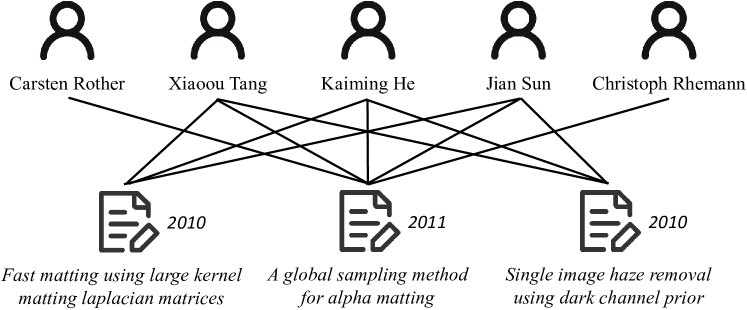
Figure 12. Case study (2): finding the time-window of the closest collaboration.

Another direct application of HBCC is identifying time-windows during which close collaborations exist within a specific research community. However, this requires a large number of queries of historical butterfly counts by enumerating both ends of the candidate time windows. Therefore, we adapt GSI to find them efficiently. For instance, within Kaiming He’s 2-hop ego network, we find that the time-window with the highest HBCC is 2010 - 2011 by GSI, with the corresponding research records detailed in Figure 12. During this period, Kaiming He, Jian Sun, Xiaoou Tang, Carsten Rother, and Christoph Rhemann established a series of cohesive research collaborations, resulting in the publication of three papers. Notably, 2010 and 2011 mark the final two years of Kaiming’s Ph.D. study, with Xiaoou serving as his supervisor, further supporting the indication that this period witnessed Kaiming’s most cohesive collaborations with others.

8. CONCLUSIONS

This paper introduces the historical butterfly counting problem on temporal bipartite graphs. We propose a graph structure-aware indexing approach to facilitate efficient query processing with a tunable balance between query time and memory cost. We further theoretically prove that our approach is especially advantageous on power-law graphs, by breaking the conventional complexity barrier associated with general graphs. Extensive empirical tests show that our algorithm is up to five orders of magnitude faster than existing algorithms with controllable memory costs.

Appendix A Technical Details for Handling Duplicate Edges

In this section, we discuss the intuition and detailed analysis of Algorithm 7.

Given a butterfly or wedge $P$, we consider a subgraph $S$ constructed by choosing exactly one edge $(u,v,t)$ for each $(u,v)\in E(P)$. We denote the set of all possible $S$s by $\mathcal{S}.$ Due to duplicate edges, $|\mathcal{S}|>1.$ For each $S\in\mathcal{S}$, its active timestamp is $[l_{S},r_{S}]$ where $l_{S}=\min_{(u,v,t)\in S}t$ and $r_{S}=\max_{(u,v,t)\in S}t$. For a time-window $[t_{s},t_{e}]$, $P\in G_{[t_{s},t_{e}]}$ if and only if there exists an $S\in\mathcal{S}$ satisfying $t_{s}\leq l_{S}\leq r_{S}\leq t_{e}$. Therefore, for $S_{1},S_{2}\in\mathcal{S}$, if $l_{S_{1}}\leq l_{S_{2}}\leq r_{S_{2}}\leq r_{S_{1}}$, then $S_{1}$ is not necessary to be considered for any query time-window. In this way, we manage to reduce the number of $S$s to be stored to answer historical queries concerning $P$.

We still need to resolve the issue of overcounting. For a time-window $[t_{s},t_{e}]$, if there are multiple $S$s such that their timestamps are all included in $[t_{s},t_{e}]$, we should not count $P$ as multiple wedges or butterflies (3.4). This is the reason we consider the redefined active timestamp in 4.3. Let the reduced set of $S$s be $\{[l_{1},r_{1}],[l_{2},r_{2}],\cdots,[l_{k},r_{k}]\}$ satisfying $l_{i}<l_{i+1},r_{i}\leq r_{i+1}$ for each $1\leq i<k$. We create a redefined timestamp $[l_{i},r_{i},r_{i+1}]$ for each $1\leq i<k$ and a redefined timestamp $[l_{k},r_{k},\infty]$ for the last timestamp $[l_{k},r_{k}]$. We can see that exactly one of the redefined timestamps becomes active when $P\in G_{[t_{s},t_{e}]}:$ If there exists $1\leq i<k$ such that $r_{i}\leq t_{e}<r_{i+1}$, only $[l_{i},r_{i},r_{i+1}]$ is active. Otherwise, we have $t_{e}\geq r_{k}$. In such case, $[l_{k},r_{k},\infty]$ is active. In addition, if $P\not\in G_{[t_{s},t_{e}]},$ no redefined timestamps becomes active. For any timestamp $[l_{i},r_{i}],$ $[t_{s},t_{e}]$ does not include $[l_{i},r_{i}].$ This implies that the redefined timestamp $[l_{i},r_{i},r_{i+1}]$ (or $[l_{k},r_{k},\infty]$ when $i=k$) is not active.

Input: A list of unique timestamps on the duplicate edges between $x$ and $y$: $L_{x,y}$; A list of unique timestamps on the duplicate edges between $y$ and $z$ : $L_{y,z}$;

Output: The active intervals $A=\{[l_{i},r_{1,i},r_{2,i}]\}$ for $\left\langle x\leadsto y\leadsto z\right\rangle$

1 $L_{x,y}\leftarrow L_{x,y}\cup\{\infty\},L_{y,z}\leftarrow L_{y,z}\cup\{\infty\}$;

2 Sort $L_{x,y}$ and $L_{y,z}$ in ascending order;

3 $S\leftarrow\emptyset,i\leftarrow 1,j\leftarrow 1$;

4 if $L_{x,y}[1]\leq L_{y,z}[1]$ then

5       $i\leftarrow$ the maximum $k$ such that $L_{x,y}[k]\leq L_{y,z}[1]$;

6else

7       $j\leftarrow$ the maximum $k$ such that $L_{y,z}[k]\leq L_{x,y}[1]$;

8$l\leftarrow\infty,r\leftarrow\infty$;

9 while $i<|L_{x,y}|$ and $j<|L_{y,z}|$ do

10       $l^{\prime}\leftarrow\min(L_{x,y}[i],L_{y,z}[j]),r^{\prime}\leftarrow\max(L_{x,y}[i],L_{y,z}[j])$;

11       if $r\neq\infty$ then  $A=A\cup\{[l,r,r^{\prime}]\}$ ;

12       if $L_{x,y}[i]\leq L_{y,z}[j]$ then

13             $i\leftarrow i+1$;

14             $j\leftarrow$ the maximum $k$ such that $L_{y,z}[k]\leq L_{x,y}[i]$;

15      else

16             $j\leftarrow j+1$;

17             $i\leftarrow$ the maximum $k$ such that $L_{x,y}[k]\leq L_{y,z}[j]$;

18      $l\leftarrow l^{\prime},r\leftarrow r^{\prime}$;

19if $r\neq\infty$ then

20       $A=A\cup\{[l,r,\infty]\}$

21

return $S$;

Algorithm 7 Computing $\left\langle x\leadsto y\leadsto z\right\rangle$’s Active Timestamps

Algorithm 7 computes the active intervals for a wedge $\left\langle x\leadsto y\leadsto z\right\rangle$. Given the two timestamp sets $L_{x,y}$ and $L_{y,z}$, we will produce all necessary $S\in\mathcal{S}$ and store the redefined timestamps in $A$. We can safely assume that there is no duplicate timestamp in either $L_{x,y}$ or $L_{y,z}$. To begin with, we initialize $S$ to be $\emptyset$ (Algorithm 7). We sort $L_{x,y}$ and $L_{y,z}$ from small to large (Algorithm 7). We also insert an $\infty$ timestamp to both timestamp sets (Algorithm 7) to avoid boundary cases. We will enumerate every element in these sets, and we denote them as $L_{x,y}[i](1\leq i\leq|L_{x,y}|$ and $L_{y,z}[j](1\leq j\leq|L_{y,z}|$. Consider a pair $(i,j)$. When $L_{x,y}[i]\leq L_{y,z}[j]$, we will adjust $i$ to $i^{\prime}$ such that $L_{x,y}[i+1]>L_{y,z}[j]$. That is to say, we will adjust the smaller side as much as possible without breaking the inequality $L_{x,y}[i]\leq L_{y,z}[j]$ (Algorithm 7, Algorithm 7, Algorithm 7, and Algorithm 7). We do the same for the case which $L_{x,y}[i]>L_{y,z}[j]$ (adjusting $j$ instead). For the current enumerated pair $(i,j)$, the corresponding redefined timestamp of the wedge formed by $(x,y,L_{x,y}[i])$ and $(y,z,L_{y,z}[j])$ is $[l,r,\max(L_{x,y}[i],L_{y,z}[j])]$, where $l$ and $r$ are the minima and maxima of the two timestamps $L_{x,y}[i]$s and $L_{y,z}[j]$s in the previous iteration (Algorithm 7 and Algorithm 7). We insert it into $A$ (Algorithm 7). After inserting, we move to the next pair by increasing one of the indices $i$ or $j$. When $L_{x,y}[i]\leq L_{y,z}[j]$, by setting $i$ to $i+1$, we will have $L_{x,y}[i]>L_{y,z}[j]$ (Algorithm 7 to Algorithm 7). Then we adjust $j$ again to the largest possible value satisfying $L_{y,z}[j]\leq L_{x,y}[i]$ (Algorithm 7). If $L_{x,y}[i]>L_{y,z}[j]$, we increase $j$ and adjust $i$ instead (Algorithm 7 and Algorithm 7). The whole process will terminate when no more feasible pair needs to be enumerated (Algorithm 7). Then, all the redefined timestamps are stored in $A$. We return $A$ as the output (Algorithm 7).

Lastly, we prove that counting the number of activated redefined timestamps can be converted to computing the difference between two 2D-range counting queries.

Previously, we regarded the active timestamp as a single point in the 2-D plane and inserted it into the 2D-counting data structure. For any time-window, the answer is computed by a single query on the data structure. Under the current definition of the active timestamp, we can still efficiently answer the query using two 2D-range counting data structures $T$ and $\overline{T}$ instead. That is to say, after construction, we will be able to answer the number of redefined timestamps $[l,r_{1},r_{2}]$ satisfying $t_{s}\leq l$ and $r_{1}\leq t_{e}<r_{2}$. Specifically, for $[l,r_{1},r_{2}]$, we insert $(l,r_{1})$ and $(l,r_{2})$ into $T$ and $\overline{T}$ respectively. To count the number of active timestamps of a time-window $[t_{s},t_{e}]$, we first query $[t_{s},\infty]\times[-\infty,t_{e}]$ on both $T$ and $\overline{T}$, denoted as $num$ and $\overline{num}$ respectively. Then, we return $num-\overline{num}$ as the answer. The formal proof is as follows.

$$\sum_{P\in G}\ \sum_{[l_{i},r_{1,i},r_{2,i}]\in\tilde{\mathcal{T}}(P)}\mathbbm{1}\{l_{i}\geq t_{s}\land t_{e}\in[r_{1,i},r_{2,i})\}=$$

$$\sum_{P\in G}\ \sum_{[l_{i},r_{1,i},r_{2,i}]\in\tilde{\mathcal{T}}(P)}\mathbbm{1}\{l_{i}\geq t_{s}\land t_{e}\geq r_{1,i}\}-\mathbbm{1}\{l_{i}\geq t_{s}\land t_{e}\geq r_{2,i}\}=$$

$$\left(\sum_{P\in G}\ \sum_{[l_{i},r_{1,i}]\in\tilde{\mathcal{T}}(P)}\mathbbm{1}\{l_{i}\geq t_{s}\land t_{e}\geq r_{1,i}\}\right)-$$

$$\left(\sum_{P\in G}\ \sum_{[l_{i},r_{2,i}]\in\tilde{\mathcal{T}}(P)}\mathbbm{1}\{l_{i}\geq t_{s}\land t_{e}\geq r_{2,i}\}\right)=$$

$$T.query([t_{s},\infty]\times[-\infty,t_{e}])-\overline{T}.query([t_{s},\infty]\times[-\infty,t_{e}])$$

Proof of Lemma 4.6.

WLOG, we assume $cnt_{x,y}\leq cnt_{y,z}$. It is easy to see the time complexity of Algorithm 7 is $O(|S|\log m)$, and we will then show $|S|\leq 3cnt_{x,y}$.

For each wedge $\left\langle x\leadsto y\leadsto z\right\rangle[l_{i},r_{1,i},r_{2,i}]\in S$, we have at least one of $l_{i}$ or $r_{1,i}$ comes from a timestamp of $L_{x,y}$. In other words, for each pair $(l,r)$ in lines 7 to 7 of Algorithm 7, there exists an $i\in[1,cnt_{x,y}]$ such that at least one of $l$ or $r$ equals to $L_{x,y}[i]$. We consider these cases as follows:

• $l=L_{x,y}[i],r\neq L_{x,y}[i]$: We move $i\leftarrow i+1$ in the next iteration, which implies this case will only occur for at most $cnt_{x,y}$ times.

• $l\neq L_{x,y}[i],r=L_{x,y}[i]$: let $\hat{l}$ and $\hat{r}$ be the values of $l$ and $r$ in the next iteration, respectively. We have $\hat{r}\geq\hat{l}\geq r$, which implies this case will only occur for at most $cnt_{x,y}$ times.

• $l=L_{x,y}[i],r=L_{x,y}[i]$: let $\hat{l}$ and $\hat{r}$ be the value of $l$ and $r$ in the next iteration, respectively. We have either $r^{\prime}\geq\hat{l}>r$ or $\hat{r}>\hat{l}\geq r$, which implies this case will only occur for at most $cnt_{x,y}$ times.

Since each wedge belongs to one of the three cases above, we prove that $|S|\leq 3cnt_{x,y}$.

∎

Appendix B Omitted Proof for Power-law Graphs

Proof for Theorem 5.1 and Theorem 5.2.

For completeness, we include the proof sketch.

By Theorem 4.5, we know that the query time for GSI is nearly linear in the number of keys $(x,z)$ in $T_{C}.$ The space usage for GSIis bounded by the number of butterflies not maintained by $T_{C}[(x,z)]$, plus the total number of wedges in each $W[(x,z)]$ for $(x,z)\in T_{C}.keys().$

To bound the query time and space usage, let $k$ be a parameter between $1$ and $\Delta=\max(\Delta_{1},\Delta_{2})$. Let $P_{\geq k}$ be the set of unordered pairs $(x,z)$ such that $x,z$ are on the same side of the bipartite graph $G$, and that $d_{x},d_{z}\geq k$. Let $\#\Join_{\geq k}$ be the number of butterflies $B$ such that $\exists\{x,z\}\in P_{\geq k}$, $\{x,z\}\subseteq B$. Here we abuse notation and use $B$ to mean the vertices of a butterfly $B$.

In Algorithm 5 of Algorithm 5, we construct $T_{C}[(x,z)]$s for pairs $(x,z)$ with the largest $W[(x,z)]$s until the total number of butterflies in these largest $W[(x,z)]$s exceeds $(1-\alpha)numB$. The rest of the butterflies will be maintained by $T_{E}.$

Intuitively, for proving the efficiency of GSI, we would like to show that a small number of $\{x,z\}$ (those in $P_{\geq k}$) covers a large fraction ($\#\Join_{\geq k}/numB$) of the total number of butterflies. Formally, we can prove that for some $k$, GSI has query complexity $\widetilde{O}(|P_{\geq k}|)$ and expected space complexity.

$O\left(\#\Join_{\geq 1}-\#\Join_{\geq k}+\sum_{(x,z)\in P_{\geq k}}|T_{C}[(x,z)]|\right)$. To show this, let’s consider an algorithm similar to Algorithm 5. The modified algorithm changes the condition on Algorithm 5 from “$num\geq\alpha\cdot numB$” to “$\{x,z\}\in P_{\geq k}$”. Then $T_{C}$ contains $|P_{\geq k}|$ elements (one for each $(x,z)\in P_{\geq k}$), and $T_{E}$ contains $\#\Join_{\geq 1}-\#\Join_{\geq k}$ butterflies. The time complexity of the modified algorithm is $\widetilde{O}(|P_{\geq k}|)$ and that the expected space usage of it is

$O\left(\#\Join_{\geq 1}-\#\Join_{\geq k}+\sum_{(x,z)\in P_{\geq k}}|T_{C}[(x,z)]|\right)$.

In the original GSI (Algorithm 5), for a fixed choice of $k$, we can choose $\alpha$ properly such that the condition on Algorithm 5 evaluates to true for the first $|P_{\geq k}|$ iterations, i.e., after the first $|P_{\geq k}|$ iterations of the loop, $num$ is no more than $\alpha\cdot numB$. The query time of GSI is bounded by $\widetilde{O}(|P_{\geq k}|).$ The space usage of GSI is bounded above by that of the modified algorithm, because the sets in $W$ are sorted with decreasing order of sizes. Each set $W[(x,z)]$ costs $|W[(x,z)]|$ space if it is maintained in $T_{C}$ and $\binom{|W[(x,z)]|}{2}$ space if it is maintained in $T_{E}$. GSI costs less space because it maintains larger sets in $T_{C}$, compared to the modified algorithm. These will automatically translates to the same bounds for GSI.

For simplicity, we use $V_{1},V_{2}$ to denote $U$, $L$. We first calculate the expected number of edges, $m$, of $G$. $m$ can be calculated by $\Delta_{i},\gamma_{i},n_{i}$ for either $i=1$ or $i=2$. For the model to be consistent, we require that the $m$’s calculated by $i=1$ and $i=2$ are equal.

Lemma B.1.

For any $i\in\{1,2\}$, if $\gamma_{i}\in(2,3)$,

$$m=\left(1+O\left(\Delta_{i}^{2-\gamma_{i}}\right)\right)\frac{n_{i}}{s_{i}(\gamma_{i}-2)}.$$

Proof.

Let $x$ be a fixed vertex in $V_{i}$.

(by linearity of expectation) $$m= n_{i}\mathbb{E}\left[\deg_{x}\right]$$

$$= n_{i}\mathbb{E}\left[d_{x}\right]$$

$$= n_{i}\frac{1}{s_{i}}\sum_{i=1}^{\Delta_{i}}i^{1-\gamma_{i}}$$

$$= \left(1+O\left(\Delta_{i}^{2-\gamma_{i}}\right)\right)\frac{n_{i}}{s_{i}(\gamma_{i}-2)}.$$

∎

Next, we estimate the expectation of $|P_{\geq k}|$ for bounding the query time.

Lemma B.2.

$\mathbb{E}\left[|P_{\geq k}|\right]=\left(1+O\left(\frac{1}{n_{1}}+\frac{1}{n_{2}}\right)\right)\left(\frac{n_{1}^{2}s_{1,k}^{2}}{2s_{1}^{2}}+\frac{n_{2}^{2}s_{2,k}^{2}}{2s_{2}^{2}}\right).$

Proof.

Recall that for any pair of vertices $x,z$, $(x,z)\in P_{\geq k}$ if $x,z\in V_{i}$ and $d_{x},d_{z}\geq k$. The expected number of such pairs for a fixed $i\in\{1,2\}$ is

$$\binom{n_{i}}{2}\mathbb{P}\left[d_{x}\geq k\right]\mathbb{P}\left[d_{z}\geq k\right]$$

$$= \binom{n_{i}}{2}\left(\frac{\sum_{d=k}^{\Delta_{d}}d^{-\gamma_{i}}}{s_{i}}\right)^{2}$$

$$= \left(1+O\left(\frac{1}{n_{i}}\right)\right)\frac{n_{i}^{2}s_{i,k}^{2}}{2s_{i}^{2}}.$$

Summing over $i=\{1,2\}$ gives

$$\mathbb{E}\left[|P_{\geq k}|\right]=\left(1+O\left(\frac{1}{n_{1}}+\frac{1}{n_{2}}\right)\right)\left(\frac{n_{1}^{2}s_{1,k}^{2}}{2s_{1}^{2}}+\frac{n_{2}^{2}s_{2,k}^{2}}{2s_{2}^{2}}\right).$$

∎

Lastly, we calculate $\mathbb{E}\left[\#\Join_{\geq k}\right],$ and $\mathbb{E}\left[\#\Join_{\geq 1}\right].$ The difference of these two numbers will bound the space usage.

Lemma B.3.

$$\mathbb{E}\left[\#\Join_{\geq k}\right]$$

$$\geq \left(1+O\left(\Delta_{1}^{\gamma_{1}-3}+\Delta_{2}^{\gamma_{2}-3}\right)\right)\frac{n_{1}^{2}n_{2}^{2}}{4m^{4}}$$

$$\frac{\left(\Delta_{1}^{3-\gamma_{1}}-k^{3-\gamma_{1}}\right)\left(\Delta_{2}^{3-\gamma_{2}}-k^{3-\gamma_{2}}\right)}{s_{1}s_{2}(3-\gamma_{1})(3-\gamma_{2})}.$$

Proof.

To get a lower bound for $\mathbb{E}\left[\#\Join_{\geq k}\right]$, we use the quantity $\#\Join_{both\geq k}$ be the number of butterflies $B=(x,y,z,w)$ such that both $(x,z)$ and $(y,w)$ are from $P_{\geq k}.$

$\#\Join_{both\geq k}$ is no more than $\#\Join_{\geq k}$ which is the number of butterflies such that at least one of $(x,z)$ and $(y,w)$ are from $P_{\geq k}.$

We sum up the probability that $x,y,z,w$ form a butterfly for $x,z\in V_{1},y,w\in V_{2}$.

$$\mathbb{E}\left[\#\Join_{both\geq k}\right]$$

$$= \binom{n_{1}}{2}\binom{n_{2}}{2}\sum_{d_{1},d_{3}\in[k,\Delta_{1}],d_{2},d_{4}\in[k,\Delta_{2}]}\mathbb{P}\left[d_{x}=d_{1}\right]\mathbb{P}\left[d_{y}=d_{2}\right]$$

$$\mathbb{P}\left[d_{z}=d_{3}\right]\mathbb{P}\left[d_{w}=d_{4}\right]\frac{d_{x}d_{y}}{m}\frac{d_{x}d_{w}}{m}\frac{d_{z}d_{y}}{m}\frac{d_{z}d_{w}}{m}$$

$$= \binom{n_{1}}{2}\binom{n_{2}}{2}\sum_{d_{1},d_{3}\in[k,\Delta_{1}],d_{2},d_{4}\in[k,\Delta_{2}]}\mathbb{P}\left[d_{x}=d_{1}\right]\mathbb{P}\left[d_{y}=d_{2}\right]$$

$$\mathbb{P}\left[d_{z}=d_{3}\right]\mathbb{P}\left[d_{w}=d_{4}\right]\frac{d_{x}^{2}d_{y}^{2}d_{z}^{2}d_{w}^{2}}{m^{4}}$$

$$= \binom{n_{1}}{2}\binom{n_{2}}{2}\frac{1}{m^{4}}\left(\sum_{d_{1},d_{3}\in[k,\Delta_{1}]}\mathbb{P}\left[d_{x}=d_{1}\right]\mathbb{P}\left[d_{z}=d_{3}\right]d_{x}^{2}d_{z}^{2}\right)$$

$$\left(\sum_{d_{2},d_{4}\in[k,\Delta_{2}]}\mathbb{P}\left[d_{y}=d_{2}\right]\mathbb{P}\left[d_{w}=d_{4}\right]d_{y}^{2}d_{w}^{2}\right)$$

$$= \binom{n_{1}}{2}\binom{n_{2}}{2}\frac{1}{m^{4}}\left(\sum_{d_{1}\in[k,\Delta_{1}]}\mathbb{P}\left[d_{x}=d_{1}\right]d_{x}^{2}\right)^{2}$$

$$\left(\sum_{d_{2}\in[k,\Delta_{2}]}\mathbb{P}\left[d_{y}=d_{2}\right]d_{y}^{2}\right)^{2}$$

$$= \binom{n_{1}}{2}\binom{n_{2}}{2}\frac{1}{m^{4}}\mathbb{E}^{2}\left[\mathbf{1}_{d_{v_{1}}\geq k}d_{v_{1}}^{2}\right]\mathbb{E}^{2}\left[\mathbf{1}_{d_{v_{2}}\geq k}d_{v_{2}}^{2}\right]$$

where $v_{1}$ ($v_{2}$) is an arbitrary vertex from $V_{1}$ ($V_{2}$). We next calculate the expectations in the equation above. For any $i\in\{1,2\}$,

$$\mathbb{E}\left[\mathbf{1}_{d_{v_{i}}\geq k}d_{v_{i}}^{2}\right]$$

$$= \sum_{d=k}^{\Delta_{i}}\mathbb{P}\left[d_{v_{i}}=d\right]d^{2}$$

$$= \frac{1}{s_{i}}\sum_{d=k}^{\Delta}d^{2-\gamma_{i}}$$

$$= \left(1+O\left(\Delta_{i}^{\gamma_{i}-3}\right)\right)\frac{\Delta_{i}^{3-\gamma_{i}}-k^{3-\gamma_{i}}}{s_{i}(3-\gamma_{i})}.$$

Thus, we have

$$\mathbb{E}\left[\#\Join_{both\geq k}\right]$$

$$= \binom{n_{1}}{2}\binom{n_{2}}{2}\frac{1}{m^{4}}\mathbb{E}^{2}\left[\mathbf{1}_{d_{v_{1}}\geq k}d_{v_{1}}^{2}\right]\mathbb{E}^{2}\left[\mathbf{1}_{d_{v_{2}}\geq k}d_{v_{2}}^{2}\right]$$

$$= \binom{n_{1}}{2}\binom{n_{2}}{2}\frac{1}{m^{4}}\Pi_{i=1}^{2}\left(1+O\left(\Delta_{i}^{\gamma_{i}-3}\right)\right)\frac{\Delta_{i}^{3-\gamma_{i}}-k^{3-\gamma_{i}}}{s_{i}(3-\gamma_{i})}$$

$$= \left(1+O\left(\Delta_{1}^{\gamma_{1}-3}+\Delta_{2}^{\gamma_{2}-3}\right)\right)\frac{n_{1}^{2}n_{2}^{2}}{4m^{4}}$$

$$\frac{\left(\Delta_{1}^{3-\gamma_{1}}-k^{3-\gamma_{1}}\right)\left(\Delta_{2}^{3-\gamma_{2}}-k^{3-\gamma_{2}}\right)}{s_{1}s_{2}(3-\gamma_{1})(3-\gamma_{2})}.$$

∎

Similar to Lemma B.3, we can estimate the expectation of $numB=\#\Join_{\geq k}.$

Lemma B.4.

$$\mathbb{E}\left[\#\Join_{\geq 1}\right]$$

$$= \left(1+O\left(\Delta_{1}^{\gamma_{1}-3}+\Delta_{2}^{\gamma_{2}-3}\right)\right)\frac{n_{1}^{2}n_{2}^{2}}{4m^{4}}$$

$$\frac{\Delta_{1}^{3-\gamma_{1}}\Delta_{2}^{3-\gamma_{2}}}{s_{1}s_{2}(3-\gamma_{1})(3-\gamma_{2})}.$$

Proof.

The proof is identical to that of Lemma B.3 with $k=1.$ We may replace the $\geq$ to $=$ because when $k=1$, $\#\Join_{both\geq k}$ is equal to $\#\Join_{\geq k}.$ ∎

Double-sided power-law bipartite graphs

In the double-sided power-law model, both $\gamma_{1}$ and $\gamma_{2}$ are in the range $(2,3)$. In this case, we have that $s_{i}$ is a constant for $i=1,2$. We also have that $m=O(n).$

We define $n=max(n_{1},n_{2})$, $\Delta=max(\Delta_{1},\Delta_{2})$, and $\gamma=min(\gamma_{1},\gamma_{2}).$

We may calculate

$\mathbb{E}\left[\#\Join_{\geq 1}-\#\Join_{\geq k}\right]$ by Lemma B.4 and Lemma B.3.

$$\mathbb{E}\left[\#\Join_{\geq 1}-\#\Join_{\geq k}\right]$$

$$= O\left(\left(\Delta_{1}^{\gamma_{1}-3}+\Delta_{2}^{\gamma_{2}-3}\right)\frac{n_{1}^{2}n_{2}^{2}}{m^{4}}\left(k^{3-\gamma_{1}}\Delta_{2}^{3-\gamma_{2}}+k^{3-\gamma_{2}}\Delta_{1}^{3-\gamma_{1}}\right)\right)$$

$$= O\left(\frac{n_{1}^{2}n_{2}^{2}}{m^{4}}\left(\left(\frac{k}{\Delta_{1}}\right)^{3-\gamma_{1}}\Delta_{2}^{3-\gamma_{2}}+\left(\frac{k}{\Delta_{2}}\right)^{3-\gamma_{2}}\Delta_{1}^{3-\gamma_{1}}+k^{3-\gamma_{1}}+k^{3-\gamma_{2}}\right)\right)$$

$$= O\left(\Delta^{6-2\gamma}\right)$$

for $k\leq\Delta.$ When $k$ is no more than the smaller of $\Delta_{1}$ and $\Delta_{2}$, we have a sharper bound.

$$\mathbb{E}\left[\#\Join_{\geq 1}-\#\Join_{\geq k}\right]$$

($$k\leq\Delta_{1},k\leq\Delta_{2} = O\left(\frac{n_{1}^{2}n_{2}^{2}}{m^{4}}\left(\Delta_{2}^{3-\gamma_{2}}+\Delta_{1}^{3-\gamma_{1}}+k^{3-\gamma_{1}}+k^{3-\gamma_{2}}\right)\right)$$)

$$= O\left(\frac{n^{4}}{m^{4}}\Delta^{3-\gamma}\right)$$

$$= O\left(\Delta^{3-\gamma}\right)$$

for $k\leq\min(\Delta_{1},\Delta_{2})$. By Lemma B.2,

$$\mathbb{E}\left[|P_{\geq k}|\right]$$

$$= O\left(n^{2}k^{2-2\gamma}\right).$$

Note that the two bounds above on space usage do not depend on $k$. Thus, we may choose the largest possible $k$ to reduce the query time in each case.

• We may choose $k=\Delta$ so that all butterflies are maintained by $T_{E}$. The query time is $\widetilde{O}(1)$ and the expected space usage is $\mathbb{E}\left[\#\Join_{\geq 1}\right]=O(\Delta^{6-2\gamma}).$

• We may also choose $k=\min(\Delta_{1},\Delta_{2})$ so that the expected query time is $\widetilde{O}(\mathbb{E}\left[|P_{\geq k}|\right])=\widetilde{O}(n^{2}\min(\Delta_{1},\Delta_{2})^{2-2\gamma})$ and the expected space usage for $T_{E}$ is $O(\Delta^{3-\gamma}).$ Note that we need to consider the space usage of $T_{C}.$ This can be bounded by

  $$\sum_{i=1}^{2}n_{i}\mathbb{E}\left[\deg_{x_{i}}^{2}\right]$$

  $$= \sum_{i=1}^{2}n_{i}\frac{\sum_{d=1}^{\Delta_{i}}d^{2-\gamma_{i}}}{s_{i}}$$

  $$= O\left(\sum_{i=1}^{2}n_{i}\Delta_{i}^{3-\gamma_{i}}\right)$$

  $$= O\left(n\Delta^{3-\gamma}\right)$$

  where $x_{i}\in V_{i}$ for $i=1,2.$ The total expected space usage is $O\left(n\Delta^{3-\gamma}\right).$

Single-sided power-law bipartite graphs

In the single-sided power-law model, we have $\gamma_{1}\in(2,3)$, $\gamma_{2}=0$, and $\Delta_{1}>\Delta_{2}.$ In this case, $s_{1}$ is a constant and $s_{2}=\Delta_{2}$. We also have that $m=\Theta(n_{1})=\Theta(n_{2}\Delta_{2}).$

We define $n=max(n_{1},n_{2})$, $\Delta=max(\Delta_{1},\Delta_{2})$.We choose $\Delta_{2}<k\leq\Delta_{1}$. We may calculate $\mathbb{E}\left[\#\Join_{\geq 1}-\#\Join_{\geq k}\right]$ by Lemma B.4 and Lemma B.3.

(1) $$\mathbb{E}\left[\#\Join_{\geq 1}-\#\Join_{\geq k}\right]$$

(2) $$= O\left(\left(\Delta_{1}^{\gamma_{1}-3}+\Delta_{2}^{\gamma_{2}-3}\right)\frac{n_{1}^{2}n_{2}^{2}}{m^{4}}\left(k^{3-\gamma_{1}}\Delta_{2}^{3-\gamma_{2}}+k^{3-\gamma_{2}}\Delta_{1}^{3-\gamma_{1}}\right)\right)$$

(3) $$= O\left(\frac{n_{1}^{2}n_{2}^{2}}{m^{4}}\left(\left(\frac{k}{\Delta_{1}}\right)^{3-\gamma_{1}}\Delta_{2}^{3-\gamma_{2}}+\left(\frac{k}{\Delta_{2}}\right)^{3-\gamma_{2}}\Delta_{1}^{3-\gamma_{1}}+k^{3-\gamma_{1}}+k^{3-\gamma_{2}}\right)\right)$$

($$k\leq\Delta_{1},\Delta_{1}>\Delta_{2} = O\left(\frac{n_{2}^{2}}{m^{2}}\left(\frac{\Delta_{1}^{6-\gamma_{1}}}{\Delta_{2}^{3}}+\Delta_{2}^{3}\right)\right)$$)

($$\frac{n_{2}}{m}=\Theta\left(\frac{1}{\Delta_{2}}\right) = O\left(\Delta_{2}+\left(\frac{\Delta_{1}^{6-\gamma_{1}}}{\Delta_{2}^{5}}\right)\right).$$)

Note that the bound above does not depend on $k$. Thus, it is an upper bound of $\mathbb{E}\left[\#\Join_{\geq 1}\right]$. We may set $\alpha>1$ so that GSI maintain all butterflies in $T_{E}$. This results in an expected query time of $\widetilde{O}(1)$. ∎

References

- (1)
- Aiello et al. (2000) William Aiello, Fan Chung, and Linyuan Lu. 2000. A random graph model for massive graphs. In Proceedings of the thirty-second annual ACM symposium on Theory of computing. 171–180.
- Aksoy et al. (2017) Sinan G Aksoy, Tamara G Kolda, and Ali Pinar. 2017. Measuring and modeling bipartite graphs with community structure. Journal of Complex Networks 5, 4 (2017), 581–603.
- Boekhout et al. (2019) Hanjo D Boekhout, Walter A Kosters, and Frank W Takes. 2019. Efficiently counting complex multilayer temporal motifs in large-scale networks. Computational Social Networks 6, 1 (2019), 8.
- Brach et al. (2016) Paweł Brach, Marek Cygan, Jakub Ł\kacki, and Piotr Sankowski. 2016. Algorithmic complexity of power law networks. In Proceedings of the Twenty-Seventh Annual ACM-SIAM Symposium on Discrete Algorithms. SIAM, 1306–1325.
- Cai et al. (2024) Xinwei Cai, Xiangyu Ke, Kai Wang, Lu Chen, Tianming Zhang, Qing Liu, and Yunjun Gao. 2024. Efficient Temporal Butterfly Counting and Enumeration on Temporal Bipartite Graphs. Proc. VLDB Endow. 17, 4 (mar 2024), 657–670. https://doi.org/10.14778/3636218.3636223
- Chazelle (1988) Bernard Chazelle. 1988. A functional approach to data structures and its use in multidimensional searching. SIAM J. Comput. 17, 3 (1988), 427–462.
- Chen et al. ([n. d.]) Kaiyu Chen, Dong Wen, Wenjie Zhang, Ying Zhang, Xiaoyang Wang, and Xuemin Lin. [n. d.]. Querying Structural Diversity in Streaming Graphs. ([n. d.]).
- Chen et al. (2021) Xiaoshuang Chen, Kai Wang, Xuemin Lin, Wenjie Zhang, Lu Qin, and Ying Zhang. 2021. Efficiently answering reachability and path queries on temporal bipartite graphs. Proceedings of the VLDB Endowment (2021).
- Deng et al. (2023) Shiyuan Deng, Shangqi Lu, and Yufei Tao. 2023. Space-Query Tradeoffs in Range Subgraph Counting and Listing. In 26th International Conference on Database Theory (ICDT 2023). Schloss-Dagstuhl-Leibniz Zentrum für Informatik.
- Eubank et al. (2004a) Stephen Eubank, Hasan Guclu, VS Anil Kumar, Madhav V Marathe, Aravind Srinivasan, Zoltan Toroczkai, and Nan Wang. 2004a. Modelling disease outbreaks in realistic urban social networks. Nature 429, 6988 (2004), 180–184.
- Eubank et al. (2004b) Stephen Eubank, Hasan Guclu, VS Anil Kumar, Madhav V Marathe, Aravind Srinivasan, Zoltan Toroczkai, and Nan Wang. 2004b. Modelling disease outbreaks in realistic urban social networks. Nature 429, 6988 (2004), 180–184.
- Fang et al. (2020) Yixiang Fang, Xin Huang, Lu Qin, Ying Zhang, Wenjie Zhang, Reynold Cheng, and Xuemin Lin. 2020. A survey of community search over big graphs. The VLDB Journal 29 (2020), 353–392.
- Goldstein et al. (2017) Isaac Goldstein, Tsvi Kopelowitz, Moshe Lewenstein, and Ely Porat. 2017. Conditional Lower Bounds for Space/Time Tradeoffs. In Algorithms and Data Structures, Faith Ellen, Antonina Kolokolova, and Jörg-Rüdiger Sack (Eds.). Springer International Publishing, Cham, 421–436.
- Goldstein et al. (2019) Isaac Goldstein, Moshe Lewenstein, and Ely Porat. 2019. On the Hardness of Set Disjointness and Set Intersection with Bounded Universe. In 30th International Symposium on Algorithms and Computation (ISAAC 2019) (Leibniz International Proceedings in Informatics (LIPIcs), Vol. 149), Pinyan Lu and Guochuan Zhang (Eds.). Schloss Dagstuhl – Leibniz-Zentrum für Informatik, Dagstuhl, Germany, 7:1–7:22. https://doi.org/10.4230/LIPIcs.ISAAC.2019.7
- Guillaume and Latapy (2006) Jean-Loup Guillaume and Matthieu Latapy. 2006. Bipartite graphs as models of complex networks. Physica A: Statistical Mechanics and its Applications 371, 2 (2006), 795–813.
- Gurukar et al. (2015) Saket Gurukar, Sayan Ranu, and Balaraman Ravindran. 2015. Commit: A scalable approach to mining communication motifs from dynamic networks. In Proceedings of the 2015 ACM SIGMOD international conference on management of data. 475–489.
- He et al. (2020) Xiangnan He, Kuan Deng, Xiang Wang, Yan Li, Yongdong Zhang, and Meng Wang. 2020. Lightgcn: Simplifying and powering graph convolution network for recommendation. In Proceedings of the 43rd International ACM SIGIR conference on research and development in Information Retrieval. 639–648.
- He et al. (2017) Xiangnan He, Lizi Liao, Hanwang Zhang, Liqiang Nie, Xia Hu, and Tat-Seng Chua. 2017. Neural collaborative filtering. In Proceedings of the 26th international conference on world wide web. 173–182.
- Jha et al. (2013) Madhav Jha, Comandur Seshadhri, and Ali Pinar. 2013. A space efficient streaming algorithm for triangle counting using the birthday paradox. In Proceedings of the 19th ACM SIGKDD international conference on Knowledge discovery and data mining. 589–597.
- Kovanen et al. (2011) Lauri Kovanen, Márton Karsai, Kimmo Kaski, János Kertész, and Jari Saramäki. 2011. Temporal motifs in time-dependent networks. Journal of Statistical Mechanics: Theory and Experiment 2011, 11 (2011), P11005.
- Latapy (2008) Matthieu Latapy. 2008. Main-memory triangle computations for very large (sparse (power-law)) graphs. Theoretical computer science 407, 1-3 (2008), 458–473.
- Li et al. (2021) Rundong Li, Pinghui Wang, Peng Jia, Xiangliang Zhang, Junzhou Zhao, Jing Tao, Ye Yuan, and Xiaohong Guan. 2021. Approximately counting butterflies in large bipartite graph streams. IEEE Transactions on Knowledge and Data Engineering 34, 12 (2021), 5621–5635.
- Li et al. (2018) Yuchen Li, Zhengzhi Lou, Yu Shi, and Jiawei Han. 2018. Temporal motifs in heterogeneous information networks. In MLG Workshop@ KDD.
- Li et al. (2019) Youhuan Li, Lei Zou, M Tamer Özsu, and Dongyan Zhao. 2019. Time constrained continuous subgraph search over streaming graphs. In 2019 IEEE 35th International Conference on Data Engineering (ICDE). IEEE, 1082–1093.
- Lind et al. (2005) Pedro G Lind, Marta C Gonzalez, and Hans J Herrmann. 2005. Cycles and clustering in bipartite networks. Physical review E 72, 5 (2005), 056127.
- Liu et al. (2019b) Boge Liu, Long Yuan, Xuemin Lin, Lu Qin, Wenjie Zhang, and Jingren Zhou. 2019b. Efficient (, )-core computation: An index-based approach. In The World Wide Web Conference. 1130–1141.
- Liu et al. (2019a) Paul Liu, Austin R Benson, and Moses Charikar. 2019a. Sampling methods for counting temporal motifs. In Proceedings of the twelfth ACM international conference on web search and data mining. 294–302.
- Liu et al. (2021) Penghang Liu, Valerio Guarrasi, and Ahmet Erdem Sarıyüce. 2021. Temporal network motifs: Models, limitations, evaluation. IEEE Transactions on Knowledge and Data Engineering 35, 1 (2021), 945–957.
- Locicero et al. (2021) Giorgio Locicero, Giovanni Micale, Alfredo Pulvirenti, and Alfredo Ferro. 2021. TemporalRI: a subgraph isomorphism algorithm for temporal networks. In Complex Networks & Their Applications IX: Volume 2, Proceedings of the Ninth International Conference on Complex Networks and Their Applications COMPLEX NETWORKS 2020. Springer, 675–687.
- Milo et al. (2002) Ron Milo, Shai Shen-Orr, Shalev Itzkovitz, Nadav Kashtan, Dmitri Chklovskii, and Uri Alon. 2002. Network motifs: simple building blocks of complex networks. Science 298, 5594 (2002), 824–827.
- Opsahl (2013) Tore Opsahl. 2013. Triadic closure in two-mode networks: Redefining the global and local clustering coefficients. Social networks 35, 2 (2013), 159–167.
- Paranjape et al. (2017) Ashwin Paranjape, Austin R Benson, and Jure Leskovec. 2017. Motifs in temporal networks. In Proceedings of the tenth ACM international conference on web search and data mining. 601–610.
- Pashanasangi and Seshadhri (2021) Noujan Pashanasangi and C Seshadhri. 2021. Faster and generalized temporal triangle counting, via degeneracy ordering. In Proceedings of the 27th ACM SIGKDD Conference on Knowledge Discovery & Data Mining. 1319–1328.
- Pavlopoulos et al. (2018) Georgios A Pavlopoulos, Panagiota I Kontou, Athanasia Pavlopoulou, Costas Bouyioukos, Evripides Markou, and Pantelis G Bagos. 2018. Bipartite graphs in systems biology and medicine: a survey of methods and applications. GigaScience 7, 4 (2018), giy014.
- Redmond and Cunningham (2013) Ursula Redmond and Pádraig Cunningham. 2013. Temporal subgraph isomorphism. In Proceedings of the 2013 IEEE/ACM International Conference on Advances in Social Networks Analysis and Mining. 1451–1452.
- Sanei-Mehri et al. (2018) Seyed-Vahid Sanei-Mehri, Ahmet Erdem Sariyuce, and Srikanta Tirthapura. 2018. Butterfly counting in bipartite networks. In Proceedings of the 24th ACM SIGKDD International Conference on Knowledge Discovery & Data Mining. 2150–2159.
- Sanei-Mehri et al. (2019) Seyed-Vahid Sanei-Mehri, Yu Zhang, Ahmet Erdem Sariyüce, and Srikanta Tirthapura. 2019. Fleet: Butterfly estimation from a bipartite graph stream. In Proceedings of the 28th ACM International Conference on Information and Knowledge Management. 1201–1210.
- Sarpe and Vandin (2021) Ilie Sarpe and Fabio Vandin. 2021. OdeN: simultaneous approximation of multiple motif counts in large temporal networks. In Proceedings of the 30th ACM International Conference on Information & Knowledge Management. 1568–1577.
- Sheshbolouki and Özsu (2022) Aida Sheshbolouki and M Tamer Özsu. 2022. sGrapp: Butterfly approximation in streaming graphs. ACM Transactions on Knowledge Discovery from Data (TKDD) 16, 4 (2022), 1–43.
- Shi and Shun (2022) Jessica Shi and Julian Shun. 2022. Parallel algorithms for butterfly computations. In Massive Graph Analytics. Chapman and Hall/CRC, 287–330.
- Vasques Filho and O’Neale (2018) Demival Vasques Filho and Dion RJ O’Neale. 2018. Degree distributions of bipartite networks and their projections. Physical Review E 98, 2 (2018), 022307.
- Wang et al. (2006) Jun Wang, Arjen P De Vries, and Marcel JT Reinders. 2006. Unifying user-based and item-based collaborative filtering approaches by similarity fusion. In Proceedings of the 29th annual international ACM SIGIR conference on Research and development in information retrieval. 501–508.
- Wang et al. (2014) Jia Wang, Ada Wai-Chee Fu, and James Cheng. 2014. Rectangle counting in large bipartite graphs. In 2014 IEEE International Congress on Big Data. IEEE, 17–24.
- Wang et al. (2019) Kai Wang, Xuemin Lin, Lu Qin, Wenjie Zhang, and Ying Zhang. 2019. Vertex Priority Based Butterfly Counting for Large-scale Bipartite Networks. PVLDB (2019).
- Wang et al. (2020) Kai Wang, Xuemin Lin, Lu Qin, Wenjie Zhang, and Ying Zhang. 2020. Efficient bitruss decomposition for large-scale bipartite graphs. In 2020 IEEE 36th International Conference on Data Engineering (ICDE). IEEE, 661–672.
- Wang et al. (2023b) Kai Wang, Xuemin Lin, Lu Qin, Wenjie Zhang, and Ying Zhang. 2023b. Accelerated butterfly counting with vertex priority on bipartite graphs. The VLDB Journal 32, 2 (2023), 257–281.
- Wang et al. (2023a) Zhibin Wang, Longbin Lai, Yixue Liu, Bing Shui, Chen Tian, and Sheng Zhong. 2023a. I/O-Efficient Butterfly Counting at Scale. Proceedings of the ACM on Management of Data 1, 1 (2023), 1–27.
- Wen et al. (2022) Dong Wen, Bohua Yang, Ying Zhang, Lu Qin, Dawei Cheng, and Wenjie Zhang. 2022. Span-reachability querying in large temporal graphs. The VLDB Journal (2022), 1–19.
- Wu et al. (2022) Shiwen Wu, Fei Sun, Wentao Zhang, Xu Xie, and Bin Cui. 2022. Graph neural networks in recommender systems: a survey. Comput. Surveys 55, 5 (2022), 1–37.
- Xie et al. (2023) Haoxuan Xie, Yixiang Fang, Yuyang Xia, Wensheng Luo, and Chenhao Ma. 2023. On querying connected components in large temporal graphs. Proceedings of the ACM on Management of Data 1, 2 (2023), 1–27.
- Yang et al. (2021) Yixing Yang, Yixiang Fang, Maria E Orlowska, Wenjie Zhang, and Xuemin Lin. 2021. Efficient bi-triangle counting for large bipartite networks. Proceedings of the VLDB Endowment 14, 6 (2021), 984–996.
- Yu et al. (2021) Michael Yu, Dong Wen, Lu Qin, Ying Zhang, Wenjie Zhang, and Xuemin Lin. 2021. On querying historical k-cores. Proceedings of the VLDB Endowment (2021).
- Zhang et al. (2023) Fangyuan Zhang, Dechuang Chen, Sibo Wang, Yin Yang, and Junhao Gan. 2023. Scalable Approximate Butterfly and Bi-triangle Counting for Large Bipartite Networks. Proceedings of the ACM on Management of Data 1, 4 (2023), 1–26.
- Zhou et al. (2021) Alexander Zhou, Yue Wang, and Lei Chen. 2021. Butterfly counting on uncertain bipartite graphs. Proceedings of the VLDB Endowment 15, 2 (2021), 211–223.
- Zou (2016) Zhaonian Zou. 2016. Bitruss decomposition of bipartite graphs. In International conference on database systems for advanced applications. Springer, 218–233.