Nexus: A framework for simulations of idealised galaxies

Abstract

Motivated by the need for realistic, dynamically self-consistent, evolving galaxy models that avoid the inherent complexity of full, and zoom-in, cosmological simulations, we have developed Nexus, an integral, flexible framework to create synthetic galaxies made of both collisionless and gaseous components. Nexus leverages the power of publicly available, tried-and-tested packages: i) the stellar-dynamics, action-based library agama; and ii) the Adaptive Mesh Refinement, N-body/hydrodynamical code ramses, modified to meet our needs. In addition, we make use of a proprietary module to account for realistic galaxy formation (sub-grid) physics, including star formation, stellar feedback, and chemical enrichment. As a framework to perform controlled experiments of idealised galaxies, Nexus’ basic functionality consists in the generation of bespoke initial conditions (ICs) for any desired galaxy model, which are advanced in time to simulate the system’s evolution. The fully self-consistent ICs are generated with a distribution-function based approach, as implemented in the galaxy modelling module of agama – up to now restricted to collisionless components, extended in this work to treat two types of gaseous configurations: (i) hot halos; and (ii) gas disks. For the first time, we are able to construct equilibrium models with disc gas fractions in the range $0<f_{\rm gas}<1$, needed to model high-redshift galaxies. The framework is ideally suited to the study of galactic ecology, specifically how stars and gas work together over billions of years. As a validation of our framework, we reproduce - and improve upon - several isolated galaxy model setups reported in earlier studies. Finally, we showcase Nexus by presenting an interesting type of ‘nested bar’ galaxy class. Future upgrades of Nexus will include magneto-hydrodynamics and highly energetic particle (‘cosmic ray’) heating.

-

1 Introduction

The study of the structure and evolution of galaxies can be approached in three different but complementary ways: 1) by direct observation; 2) by theoretical work; 3) by simulation. In the last case, most of the work falls on one of two broad categories: That where the evolution of a significant volume of the Universe is considered – so-called ‘large-scale structure’ or ‘cosmological’ simulations , and at the other end, that where the evolution of individual (isolated) systems is looked at, henceforth referred to as ‘constrained’ simulations.

Cosmological simulations have greatly helped advance our understanding of galaxy formation (for an extensive review see Naab & Ostriker, 2017). The core idea is to evolve gravitationally the inhomogeneities imposed at the start of the simulation on an otherwise uniform matter distribution, which are consistent with the quantum fluctuations in the nascent Universe (Zeldovich, 1970). Together with the use of a number of ‘recipes’ to mimic otherwise unresolved physical processes believed to be key in shaping galaxies (e.g. star formation and stellar feedback, black-hole accretion, chemical enrichment, radiative cooling at atomic scales, cosmic ray production, etc.) this approach allows us to calculate from ‘first principles’ how galaxies with properties astonishingly similar to real galaxies – statistically speaking – emerge across cosmic time (e.g. Schaye et al., 2015; Dubois et al., 2016; Grand et al., 2017; Dolag et al., 2017; Pillepich et al., 2018).

However remarkable, cosmological simulations also have limitations. The most crucial ones are perhaps: 1) a relatively low resolution (both spatially and in terms of particle sampling), and 2) that they offer no real control over the galaxy properties of interest. Note that while so-called cosmological ‘zoom’ simulations (e.g. Nuza et al., 2014; Hopkins et al., 2014; Kim et al., 2014; Wetzel et al., 2016; Agertz et al., 2021) do allow for a significant improvement in resolution, they do not mitigate the second issue. For instance, in the study of systems with very specific properties, e.g. Milky-Way (MW) ‘analogues’, compromises have to be made because it is virtually impossible to find systems that satisfy the required constraints (e.g. a galaxy with DM halo, stellar and gas discs, and bulge masses matching those of the MW within their uncertainties). This is even more severe if one aims at finding systems that are nearly identical but in one or two aspects, say two MW ‘twins’ that differ only in their age or their accretion history (but see Roth et al., 2016; Rey & Pontzen, 2018). In a nutshell, cosmological simulations allow for robust statistical analyses of galaxy properties, but are less useful when it comes to study in detail specific systems (e.g. the MW or Andromeda, to name a few).

To overcome this problem, there exists an alternative approach, which consists in the use of controlled experiments, whereby initial conditions for individual (and generally isolated) galaxies with very specific properties (e.g. mass, size, structure, etc.) – thus referred to as ‘idealised’, can be constructed, and evolved under different conditions. By systematically varying one of the relevant features of the model (e.g. the disc mass) or the way it is evolved (e.g. adiabatic vs. cooling / heating) – a powerful approach we refer to as ‘differential’ – one can isolate the effect of that feature on the overall response of the system (e.g. Athanassoula, 1992; Hernquist, 1993; Wada & Norman, 2001; Di Matteo et al., 2005; Agertz et al., 2009a; Hopkins et al., 2011; Grisdale et al., 2017; Renaud et al., 2021; van Donkelaar et al., 2022). It is important to emphasise that these controlled experiments cannot explain how galaxies form, only (at best) how they evolve in an environment devoid of the boundary conditions (inflows, large-scale gravitational potential, etc.) provided by cosmological simulations, starting from somewhat ad hoc initial conditions (hence ‘idealised’).

Needless to say, these approaches – cosmological simulations, zoom-in simulations, and constrained experiments of idealised galaxies – are all complementary to each other.

A requirement to perform controlled simulations is the existence of a method (or a framework) that allows to create galaxy models that: 1) can be tailored to specific needs in a flexible way; and crucially, 2) are physically self-consistent in the sense that the properties of the system (total potential, mass distribution, velocity distribution) are consistent with one another. In addition, it should allow setting up models that are sometimes in stable equilibrium from the outset (e.g. Bland-Hawthorn & Tepper-García, 2021), or unstable in a controlled way (e.g. Fujii et al., 2018).

1.1 A new framework

A review of the literature reveals that there is a wealth of methods and implementations (in the form of software) available to accomplish the task of setting up an idealised galaxy. However, those that allow to initialise systems containing both collisionless and gas components are rare; notable exceptions are: Make[New]disc (Springel et al., 2005), the disc Initial Conditions Environment (DICE; Perret et al., 2014; Perret, 2016), or GalactICs+Gas (Widrow et al., 2008; Deg et al., 2019), all of which are still highly in demand (cf. D’Onghia & L. Aguerri, 2020; de Sá-Freitas et al., 2023; Anderson et al., 2022, respectively)

Perhaps the lack of adequate, accessible frameworks explains in part the mild aversion of many galactic dynamicists/simulators to consider galaxy models that include a gaseous component. In none but very few cases is this omission justified, even less so when the goal is to interpret observational data of specific systems, for instance, the origin of the Gaia phase spiral (e.g. Laporte et al., 2019; Bland-Hawthorn & Tepper-García, 2021; Hunt et al., 2021, Tepper-García et al, in prep.). The importance of including gas when studying galaxy structure – in addition to the obvious reason that stars form out of gas – has been unambiguously expressed by Binney & Tremaine (2008), citing a statement attributed to Oort: “The principal features that distinguish lenticular or S0 galaxies from spirals are the low density of cold interstellar gas, the absence of young stars, and the absence of spiral arms. Only a tiny fraction of gas-poor disc galaxies exhibit spiral arms […] Thus, even though spiral structure is present in the old disc stars, interstellar gas is essential for persistent spiral structure” (see also D’Onghia et al., 2013).

Overall, it is striking that among the available frameworks to initialise idealised galaxies only a few follow a distribution function (DF) based approach to fulfil this task (e.g. GalactICs), the only approach that yields fully self-consistent results.

Indeed, a recurrent issue with simulations of idealised galaxies has been that the initially specified, multi-component system is not in equilibrium, and thus evolves to a new configuration before long-term stability is achieved; the simulator must then accept a model that is substandard and not what was specified. This has been a longstanding problem that a DF-based approach, as implemented in GalactICs or the Action-based Galaxy Modelling Architecture (agama) library (Vasiliev, 2019), inherently avoids.

In its original form, GalactICs only allowed to generate ICs for collisionless components, appropriate to model systems made of e.g. dark matter and stars. Given the need for more realistic galaxy models that incorporate gas, the library was later extended (Deg et al., 2019). The situation is analogous with the agama library, which in its standard form does not allow including responsive gas components.

This is a shortcoming our present paper is set out to remedy. Taking full advantage of the library’s framework, here we expand the agama self-consistent modelling (SCM) module to treat gas components in addition to the already included collisionless ones. This is a major innovative step that allows to construct $N$-body/hydrodynamical models of galaxies that are fully self-consistent, and therefore in equilibrium, from the outset. As is the case with the GalactICs+Gas code, we anticipate that this extension of the agama library will become useful to the astrophysical community working with these type of simulations.

In fact, our group has already made use of our extended agama framework in several instances (Tepper-García et al., 2022; Bland-Hawthorn et al., 2023, 2024, Davis et al., in prep.; Tepper-Garcia et al., in prep.), and others have followed with a similar approach (Annem & Khoperskov, 2024). The main purpose of the present paper is to formally introduce and explain our methodology – only briefly described in our early papers –, as well as provide a reference for future work, providing many details that in other studies are only glossed over.

The structure of this paper is as follows: Sec. 2 describes some of the methods used to create equilibrium galactic gas configurations. Sec. 3 describes our implementation of a subset of these methods within the agama library. In Sec. 4 we briefly describe the modifications to the ramses code required by our framework, including our adopted implementation of galaxy-formation physics. In Sec. 5 we validate our method with a number of simple test cases, and discuss a case of astrophysical interest in Sec. 6. We conclude with a reflection about the importance of controlled experiments of idealised galaxies in Sec. 7.

2 Idealised, gaseous galactic components

In what follows, we present an overview of some of the most common approaches put forward in the literature to construct equilibrium galactic gas configurations (cf. Recchi, 2014). Specifically, we focus on models of galactic hot halos (or ‘coronae’) and galactic gas discs. Throughout, we limit our scope to ideal, mono-atomic gases. We refrain from discussing the setup of collisionless components with agama, which has been discussed at length elsewhere (cf. Bland-Hawthorn & Tepper-García, 2021; Tepper-Garcia et al., 2021; Tepper-García et al., 2022; Bland-Hawthorn et al., 2023).

2.1 Galactic coronae

Originally predicted by Spitzer (1956) as the confining medium behind H i clouds in the Galactic halo, and later by early theories of galaxy formation (Binney, 1977; White & Rees, 1978), hot gas halos have now been firmly established, at least in a handful of systems, including the Milky Way (Miller et al., 2016), Andromeda (Lehner et al., 2017), and most recently the Magellanic Clouds (Krishnarao et al., 2022). This suggests that nearly every galaxy in the Universe is likely to be embedded within a hot corona (for a comprehensive review, see Bregman et al., 2018).

The importance of galactic coronae cannot be overstated. They are believed to constitute significant gas reservoirs from which galaxies may obtain sufficient gas supply to maintain relatively high star formation over cosmologically relevant time scales (e.g. Marinacci et al., 2010; Grønnow et al., 2018). In addition, they are a dynamically important component, which also affects the accretion of gas onto the star-forming disc delivered through cosmological filaments (Stern et al., 2024) or via tidal disruption of satellites (Mastropietro et al., 2005; Tepper-García & Bland-Hawthorn, 2018b; Tepper-García et al., 2019). Also, galactic coronae may be key in providing a solution to the ‘missing baryons’ at low redshift (Fukugita & Peebles, 2006). Finally, they provide external pressure onto the dense interstellar medium (ISM), leading to a more complex disc-halo interactive interaction.

In short, galactic coronae are a physical reality and a necessary ingredient in any realistic galaxy model, and yet they are generally ignored. This deficiency of many idealised galaxy models is one of the many we intend to address with our new framework.

2.1.1 Halo density structure and internal energy

Hot halos are often – out of convenience – assumed to be spherical, isothermal gas configurations with a temperature $T$ in hydrostatic equilibrium (HSE) with the total galactic potential $\Phi$ (Sutherland & Bicknell, 2007). In this case, their density structure as a function of the spherical radius $r=\sqrt{R^{2}+z^{2}}$ – with $R$ and $z$ the cylindrical coordinates – is described by

$$\rho_{\rm gh}(r)=\rho_{0}\leavevmode\nobreak\ \exp\left\{\Phi(R,z)/c^{2}_{s}\right\}\,.$$ (1)

Here, $\rho_{0}$ is the central density, $c^{2}_{s}=k_{b}T/\mu\leavevmode\nobreak\ m_{p}$ is the isothermal sound speed, and $\Phi\leq 0$.

However, such models are far from realistic, as suggested both by observations (Hodges-Kluck et al., 2018) and cosmological simulations (Oppenheimer, 2018). Yet, they are very useful for the purposes of validating a code aimed at creating such configurations, given that the analytic solution is known, with the potential caveat that HSE is notoriously difficult to maintain in fluid dynamics (grid) codes (Käppeli & Mishra, 2016; Krause, 2019; Canivete Cuissa & Teyssier, 2022).

Less restrictive, and at the same time more realistic, models correspond to spherical configurations described by a density $\rho_{\rm gh}(r)$ in HSE with the total potential, but not necessarily isothermal. For these, the temperature profile can be obtained from the Jeans (1915) equation for a spherically symmetric system,

$$\sigma^{2}_{r}(r)=\frac{1}{\rho_{\rm gh}}\int_{r}^{\infty}\rho_{\rm gh}\frac{\partial\Phi}{\partial r^{\prime}}dr^{\prime}\,,$$ (2)

where the (no longer constant) sound speed is set identical to the macroscopic velocity dispersion, i.e. $c^{2}_{s}\equiv\sigma^{2}_{r}$ (cf. Mastropietro et al., 2005), implying a (spherically symmetric) temperature profile

$$T_{\rm HSE}(r)=\frac{\mu\leavevmode\nobreak\ m_{p}}{k_{b}}\sigma^{2}_{r}(r)\,.$$ (3)

Yet more realistic models correspond to partially pressure-supported, spinning coronae (Barnabè et al., 2006; Pezzulli et al., 2017; Sormani et al., 2018) in vertical hydrostatic equilibrium (vHSE; $v_{z}\equiv 0$), in which the temperature at any given radius is dictated by the balance between the hydrostatic pressure support and the streaming velocity $v_{\phi}$,

$$T_{\rm rot}(r)=T_{\rm HSE}(r)-\frac{1}{2}(1-\gamma)\frac{\mu\leavevmode\nobreak\ m_{p}}{k_{b}}v^{2}_{\phi}\,.$$ (4)

Here, $\gamma$ is the adiabatic index and is equal to 5/3 for a mono-atomic gas. This factor appears because the balance between pressure and rotational support is obtained in terms of the specific internal energy of the gas,

$$e=c^{2}_{s}/(1-\gamma)\,.$$

Thus, the model is fully specified once $\rho$ and $v_{\phi}$ are.

At galactic scales, this last type of models is certainly the most relevant, and for this reason they form the basis of the corona models included in our framework.

It is worth noting that the approach outlined above always yields spherically symmetric configurations. However, spinning coronae will flatten, adopting an oblate or even a toroidal geometry (e.g. Tepper-García & Bland-Hawthorn, 2018b). Such models can be setup from the outset (e.g. Pezzulli et al., 2017; Sormani et al., 2018), but we leave these cases for future versions of Nexus.

2.1.2 Halo velocity structure

In the case of spinning coronae in vHSE, only the $v_{x}$- and $v_{y}$ velocity components need to be specified, which in turn requires knowledge of the streaming (azimuthal) velocity $v_{\phi}$. The latter is however not constrained in any way by the Jeans (1915) equations, and can thus be freely chosen.

Different approaches have been adopted in the past. A widely used approach, pioneered by Strickland & Stevens (2000), relies on setting $v_{\phi}=ev_{c}$, where $0<e<1$ and $v^{2}_{c}=R\leavevmode\nobreak\ \partial\Phi/\partial R$ is the total circular speed of the system (e.g. Barbani et al., 2023).

A different, more physically motivated, approach involves assuming a self-consistent centrifugal support where the velocity is obtained by solving for $v_{\phi}$, given a density $\rho$ and an equation of state $P(\rho)$ (e.g. D’Ercole & Brighenti, 1999).

Yet another common approach, motivated from cosmology, is based on the following idea. Tidal torque theory suggests that a collapsing DM halo (and the baryons within) acquire angular momentum ($J$) as a result of a misaligned (i.e. not perfectly radial) infall (Hoyle et al., 1949; White & Rees, 1978; Efstathiou & Jones, 1979; Fall & Efstathiou, 1980). The specific angular momentum $j\equiv J/M$ of the virialised system of total mass $M$ (DM halo and baryons) can be indirectly parameterised by the ‘oblatness’ (Peebles, 1969), more popularly known as ‘spin parameter’ (Mo et al., 1998),

$$\lambda^{2}\equiv\frac{j^{\,2}\leavevmode\nobreak\ |E|}{G^{2}\leavevmode\nobreak\ M^{3}}\,,$$ (5)

where $E$, is the sum of potential, kinetic and thermal energies.

The core idea is that the DM halo and the baryons within have a spin determined by either $\lambda$ or $j$, which is in turn set by the fundamental properties ($M$, $E$) of the collapsing system. For instance, cosmological, DM-only simulations of structure formation (Bullock et al., 2001) suggest that $j\propto M^{s}$ with $s=1.3\pm 0.3$, where $M$ is the total mass enclosed within $r$. It can be shown that such a behaviour derives from an exponential angular momentum distribution (AMD), $\psi(l)\propto(M/l)\leavevmode\nobreak\ e^{-l/l_{0}}$ (Sharma et al., 2012).

Estimates from $\lambda$ are also obtained from these simulations, which indicate that DM halos have spin parameters that roughly follow a log-normal distribution with its peak at approximately $0.035\pm 0.005$ and width $0.5\pm 0.03$ (Bullock et al., 2001).

All of the above results apply to DM halos only. However, full hydro-cosmological simulations indicate that the spin of (hot) gas accreting onto a DM halo displays the same behaviour with mass, but with a different (larger) normalisation, up to factors 3 compared to the DM, i.e. $\langle\lambda_{gas}\rangle\approx 0.12$ (Pichon et al., 2011).

Future versions of Nexus may introduce alternative, potentially better, approaches, in particular, those suitable to set up initially flattened halos (see e.g. Sormani et al., 2018).

2.2 Galactic gas discs

Settled, galactic gas discs are generally observed to follow an exponentially declining surface density with a characteristic scale length $R_{d}$ (Leroy et al., 2009; Kalberla & Kerp, 2009),

$$\Sigma(R)=\Sigma_{0}\exp\{-R/R_{d}\}\,.$$ (6)

Thus, many of the approaches in the literature used to set up isolated, galactic gas discs assume an exponentially declining profile; the vast majority of them follow the method pioneered by Springel, Di Matteo & Hernquist (2005). In essence, their approach consists in solving the steady-state momentum conservation equation for a perfectly axi-symmetric ($\partial/\partial\phi\equiv 0$), rotationally supported ($v_{R}\equiv 0$) disc in vertical hydrostatic equilibrium ($v_{z}\equiv 0$),

$$\frac{1}{\rho}\frac{\partial P}{\partial R}+\frac{\partial\Phi}{\partial R} =\frac{v_{\phi}^{2}}{R},$$ (7)

$$\frac{1}{\rho}\frac{\partial P}{\partial z}+\frac{\partial\Phi}{\partial z} =0\,,$$ (8)

for the density $\rho(R,z)$, given a total galactic potential, $\Phi$, and a specified equation of state $P(\rho)$.

Here, we adopt an alternative approach, introduced by Wang et al. (2010). These authors developed a simple, effective, and computationally efficient method to arrive at a solution for the special case of an isothermal, ideal gas disc, characterised by the equation of state $P(\rho)=c_{s}^{2}\leavevmode\nobreak\ \rho$ with a constant sound speed $c_{\mathrm{s}}$. Although their method is valid only for isothermal configurations (if one is interested in equilibrium systems), it also serves well to set up more general systems, for example, when using the model as a starting point for a system that is allowed to undergo cooling and heating, and to form stars.

In what follows, we briefly outline the method put forward by Wang et al. (2010). In Sec. 3.4, we detail how the algorithm is modified to meet our needs.

2.2.1 disc density structure

If the disc is made up of an isothermal, ideal gas, then $c_{s}$ is a constant, and Eq. (8) can be readily integrated to yield the gas volume density,

$$\rho(R,z)=\rho_{0}(R)\leavevmode\nobreak\ \rho_{z}(R,z)\,,$$ (9)

where

$$\rho_{z}(R,z)\equiv\exp\left\{-\Phi_{z}/c^{2}_{s}\right\}\,,$$ (10)

and

$$\Phi_{z}(R,z)\equiv\Phi(R,z)-\Phi(R,0)\,.$$ (11)

Integrating Eq. (9) over $z$ yields the gas surface density,

$$\Sigma(R)=\int_{-\infty}^{+\infty}\!\!\!\!\!\rho(R,z)\leavevmode\nobreak\ dz=2\leavevmode\nobreak\ \rho_{0}(R)\!\!\int_{0}^{+\infty}\!\!\!\!\!\rho_{z}(R,z)\leavevmode\nobreak\ dz\,,$$ (12)

where in the last step it is assumed that the potential, and thus the volume density, is symmetric with respect to the mid-plane. Clearly, both $\rho_{0}$ and $\rho_{z}$ should be such that the above result agrees with Eq. (6).

Mathematically, the factor $\rho_{0}$ in Eq. (12) is a constant of integration, which physically corresponds to the mid-plane gas density; it can be expressed as

$$\rho_{0}(R)=\frac{1}{2}\Sigma(R)\left[\int_{0}^{+\infty}\rho_{z}(R,z)\leavevmode\nobreak\ dz\right]^{-1}\,.$$ (13)

Modelling the structure of a realistic gas disc thus reduces to the problem of finding $\rho(R,z)$ for a given $\Sigma(R)$, and a corresponding $\Phi_{g}$ via Poisson’s equation,

$$\nabla^{2}\Phi_{g}=4\pi G\,\rho\,,$$ (14)

such that Eqs. (9 – 13) are all self-consistent. Here, $\Phi_{g}$ is the contribution of the gas disc to the total potential of the system,

$$\Phi=\Phi_{g}+\sum_{i}\Phi_{i}\,,$$ (15)

where $\Phi_{i}$ are any other galaxy components (e.g. DM halo, stellar bulge, stellar disc, etc.).

Wang et al. (2010) describe an iterative, efficient algorithm to accomplish this task, as follows:

1. Fix $\Sigma(R)$ and choose initial contributions $\Phi_{i}$ to $\Phi$ (Eq. 15),

2. Choose initial guesses for $\rho_{z}(R,z)$ and $\rho_{0}(R)$,

3. Calculate $\rho(R,z)$ via Eq. (9) and $\Phi_{g}(R,z)$ via Eq. (14),

4. Calculate $\rho_{z}(R,z)$ via Eq. (10),

5. Calculate a new $\rho_{0}(R)$ via Eq. (13),

6. Go to step 3 and repeat until convergence.

In this context, ‘convergence’ can be measured for example by tracking the change in the value of the central density $\rho_{0}(R=0)$ and demanding it falls below some prescribed threshold, say 1 percent. In such a case, the iterative process converges in a few iterations, provided a suitable choice is made for the initial guess $\rho_{0}(R)$. For instance, Wang et al. (2010) recommend setting $\rho_{0}(R)\propto\Sigma(R)$, which works remarkably well.

As anticipated by Deg et al. (2019), the above algorithm can be seamlessly integrated into agama’s self-consistent modelling iterative procedure, which we describe later in Sec. 3.

2.2.2 disc velocity structure

Once the density profile has been fixed, the magnitude of the streaming (azimuthal) velocity of the gas follows from Eq. (7),

$$v^{2}_{\phi}=\frac{R}{\rho}\frac{\partial P}{\partial R}+v^{2}_{c}\,.$$ (16)

Since $P$ (and $\rho$) generally decreases with radius for an exponential disc, the streaming gas velocity is the result of the balance between the pressure gradient and the centrifugal force induced by the total galactic potential $\Phi$. In other words, once the density structure of the disc and the total potential of the self-consistent model are known, $v_{\phi}$ is fully determined by Eq. (16).

Whilst in general the gas rotation velocity is dependent both on the cylindrical radius, $R$, and the height from the mid-plane, $z$ (Barnabè et al., 2006), it depends only on $R$ for barotropic (i.e. $P=P(\rho)$) configurations (Poincaré-Wavre theorem; q.v. Lebovitz, 1967), which include isothermal configurations as a special case. Thus, for all our intents and purposes, Eq. (16) defines the rotation velocity for any $z$, i.e.  $v_{\phi}(R,z)\equiv v_{\phi}(R)$ .

3 Implementation in AGAMA

In the following we describe our implementation in agama of the approaches discussed above. We start by providing a brief overview of the relevant theory underlying the DF-based approach to set up initial conditions for isolated galaxy models, with an emphasis on the iterative nature of the problem, and explain how we exploit it to meet our needs. More details can be found in Vasiliev (2019, or for a more concise description).

3.1 Theoretical background

The evolution of a collisionless $N$-body system with a sufficiently large number of particles is governed by the collisionless Boltzmann equation and its solution, the ‘one-particle’ distribution function, $f(\bm{r},\bm{v},t)$. In a steady state, $f(\bm{r},\bm{v},t^{\prime})\equiv f(\bm{r},\bm{v},t=0)$, for any time $t^{\prime}>0$, implying that $f$ is a function of the integrals of motion only (Jeans, 1915).

A convenient set of integrals of motion are the action variables, which in the case of axi-symmetric potentials, are the radial action $J_{R}$, the vertical action $J_{z}$, and the azimuthal action $J_{\phi}$ (equivalent to the $z$-component of the angular momentum vector).

In this case, $f=f(\bm{J})\equiv f(J_{R},J_{z},J_{\phi})$. This implies the existence of a mapping $(\bm{r},\bm{v})\mapsto\bm{J}$ that depends on the total potential of the system $\Phi$, succinctly expressed as $\bm{J}\left[\bm{r},\bm{v}\leavevmode\nobreak\ |\leavevmode\nobreak\ \Phi\right]$.

The distribution function provides a statistical description of the dynamical state of the system, and other properties can be derived from it. For example, for an appropriate normalisation, the mass density $\rho_{c}$ of a component (e.g. stellar disc) described by a DF $f_{c}$ is given by

$$\rho_{c}(\bm{r})=\int\!\!f_{c}\left\{\bm{J}\left[\bm{r},\bm{v}\leavevmode\nobreak\ |\leavevmode\nobreak\ \Phi\right]\right\}\leavevmode\nobreak\ d\bm{v}\,.$$ (17)

3.2 Self-consistent models

In agama, a fully self-consistent (not necessarily in a stable equilibrium) galaxy model with a specified number of collisionless components (e.g. halo, bulge, disc) is defined by:

• The density of each component, $\rho_{c}(\bm{r})$, calculated from its corresponding DF ($f_{c}$)

• The DF of each component, expressed in terms of actions, $f_{c}\left\{\bm{J}\left[\bm{r},\bm{v}\leavevmode\nobreak\ |\leavevmode\nobreak\ \Phi\right]\right\}$, dependent on the potential $\Phi$.

• The total potential of the system, $\Phi$, determined via the superposition of all $\rho=\sum\rho_{c}$ via Poisson’s equation $\nabla^{2}\Phi=4\pi G\rho$.

• The mapping $\bm{J}\left[\bm{r},\bm{v}\leavevmode\nobreak\ |\leavevmode\nobreak\ \Phi\right]$, for which agama makes use of the so-called ‘Stäckel fudge’ (Binney, 2012), appropriate for axi-symmetric configurations.

The relationship between these model ingredients imply a coupled system of non-linear equations that must be solved iteratively. To solve it, the self-consistent modelling (SCM) module within the agama library adopts the following ‘recipe’:

1. Specify the initial (target) density profile $\rho_{c}$ (or alternatively, the corresponding potential), of each galaxy component,

2. Specify the DF, $f_{c}(\bm{J})$, for each component; $f_{c}$ remains fixed during subsequent iterations,

3. Calculate the potential of the system via $\nabla^{2}\Phi=4\pi\sum_{c}\rho_{c}$,

4. Determine the mapping $\bm{J}\left[\bm{r},\bm{v}\leavevmode\nobreak\ |\leavevmode\nobreak\ \Phi\right]$ and recompute the new density of each component $\rho^{\prime}_{c}$ via Eq. (17),

5. Repeat the last two steps until ‘convergence’ (see below).

Convergence during the iterative process is guaranteed by the adiabatic invariant nature of actions, together with the use of $f(\bm{J})$. This can be judged, for example, by the maximum absolute change across iterations of the total potential at the origin, and ideally it should be of the order of a percent or less.

Once a converged model has been attained, an $N$-body representation of the system is created by drawing a specified number $N_{c}$ of random samples (point-like masses or ‘particles’) for each component directly from phase space $(\bm{r},\bm{v})$ by evaluating $f(\bm{J})$ using the mapping $\bm{J}\left[\bm{r},\bm{v}\leavevmode\nobreak\ |\leavevmode\nobreak\ \Phi\right]$ together with the final, self-consistent potential. To this end, agama implements an efficient multidimensional sampling-rejection algorithm. Thus, the construction of an $N$-body model with agama yields a fully self-consistent ‘potential - density - velocity distribution’ triplet.

3.3 Galactic coronae

In its standard form, agama readily allows setting up hot a halo as a fully valid, DF-based, spheroidal component, starting from a target density profile (e.g. Tepper-Garcia et al., 2021, their section 3.3.1). In essence, this is the same approach used to set up a generic spheroidal component, say, a DM halo or a classical stellar bulge. The difference is that, once the model has converged (in the sense of Sec. 3.2), a hot halo component requires some post-processing in order to arrive at a self-consistent gas configuration, as described below.

3.3.1 Initial density profile and distribution function

We focus our attention on a partially pressure-supported, spinning hot halo embedded in a DM host halo. We restrict our discussion to NFW-like galactic DM halos (Navarro et al., 1997), and assume for the sake of simplicity that an embedded hot halo follows the same profile. In doing so, we follow on the footsteps of a long list of earlier, seminal studies (e.g. Mo et al., 1998; Ascasibar et al., 2003; Mastropietro et al., 2005; Kaufmann et al., 2006; Aumer et al., 2010; Teyssier et al., 2013; Clarke et al., 2019). It is worth emphasising that our choice does not limit our framework in any way, which in fact is flexible and can easily accommodate other types of profiles.

The initial density of the hot halo is described by the following generic function,

$$\rho_{s}(r)=\rho_{0}\left(\frac{r}{r_{s}}\right)^{-\gamma}\left[1+\left(\frac{r}{r_{s}}\right)\right]^{\gamma-\beta}\times\exp{\left[-\left(\frac{r}{r_{c}}\right)^{2}\right]}\,,$$ (18)

that represents a double power-law, ‘spheroidal’ profile with a taper. Here, $r$ is the spherical radius; the other parameters have the following meaning:

• $\rho_{0}$ := density normalisation

• $r_{s}$ := scale radius

• $r_{c}$ := outer cut-off radius

• $\beta$ := outer power-law slope

• $\gamma$ := inner power-law slope

We note that this density profile is available as part of the standard agama Potential-Density Factory, and it is flexible enough to accommodate a significant number of relevant profiles (we refer the reader to the agama documentation for more details).

To arrive at a density configuration that closely (or exactly, if the hot halo is isolated) resembles a NFW profile, one must set $\beta\equiv 3$ and $\gamma\equiv 1$. The remainder of the parameters determine the mass, concentration, and extension of the halo, and they should be chosen according to the intended application.

During the iterative process, we assigned the halo a DF of the type ‘Quasi-Spherical’, well-suited to model spheroidal components. However, instead of specifying the analytic form of the DF (which is possible with agama), the DF is constructed directly from the density distribution (18) using either the Eddington inversion formula or its anisotropic generalisation (Cuddeford, 1991), which has the advantage of reducing the number of free parameters while also speeding up the calculations.

Once the mass distribution of the hot halo is fixed, all that remains to be calculated is the velocity structure and the internal energy, in that order (see Eq. 4), which is done in ‘post-processing’, i.e. using tools external to add functionality to the standard agama library.

3.3.2 Post-processing

Post-processing is accomplished with help of the pynbody package (Pontzen et al., 2013). During this procedure, the particle constituents of the hot halo are assigned a temperature $T$ (or equivalently, an internal energy $e$), which in turn requires re-adjusting the (macroscopic) velocities assigned via the self-consistent DF-based approach. Furthermore, depending on the intended application of the model, the gas may be required to have a specific metal mass fraction $Z_{met}$ (or equivalently, an elemental abundance distribution), e.g. if the gas is allowed to heat, to cool (radiatively), and to form stars (cf. Sec. 4).

It is worth stressing that, since the density distribution is not altered in any way during post-processing, the system retains its full dynamical consistency, provided the relation between velocities and temperature is self-consistent as well.

We are only interested in cosmologically motivated hot halos with properties consistent with those either predicted by galaxy formation theory or simulation. Neither, it must be noted, is able to put tight constraints on the structure of hot halos, which allows for some freedom when making a choice. In other words, the thermodynamic and kinematic properties of hot coronae are not well understood. But it may be stated with some confidence they are not isothermal and not in (nor close to) a state of hydrostatic equilibrium, at least on galactic scales (Oppenheimer, 2018; Hodges-Kluck et al., 2018), as we have assumed in previous work for the sake of simplicity (Tepper-García et al., 2015).

The assignment of a metal mass fraction or specific elemental abundance is nearly trivial as it amounts to create additional particle properties (i.e. effectively arrays) with the desired values, and it is not discussed further. In contrast, assigning a temperature profile requires calculating first the velocity structure (Eq. 4), which in turn requires some care.

As outlined in Sec. 2.1.2, the velocity structure is calculated assuming that the specific angular momentum of the gas, $j_{h}$, follows that of the dark matter (c.f. Kaufmann et al., 2006). Specifically, we adopt $s=1$, which implies

$$v_{\phi}(r)=\frac{j_{h}(r)}{r}=g_{0}\frac{M_{h}(<r)}{r}\,,$$ (19)

where $g_{0}$ is an appropriate normalisation constant to be determined.

To this end, first we need to calculate the total angular momentum, $J$, of the system. Because we are assuming the gas follows the same profile as the DM, we use the total (DM + gas) mass $M$ to calculate the viral radius $R$; we fix the value of the spin parameter $\lambda$, and calculate the energy via (Mo et al., 1998)

$$E_{\textnormal{\sc dm}}=-\frac{1}{2}\frac{GM^{2}_{\textnormal{\sc dm}}}{R_{\textnormal{\sc dm}}}f_{c}\,,$$

where

$$f_{c}=\frac{c}{2}\left[1/x^{2}-(2\ln x)/x\right]\leavevmode\nobreak\ \left[c/x^{\phantom{2}}-\ln x\right]^{-2}\,,$$

$x=1+c$, and $c=R/r_{s}$. We note that these expressions are strictly valid only for NFW halos. If the DM (or hot) halo is required to follow a different profile, then different formulae are necessary. The total angular momentum $J$ is then calculated from Eq. (5), using the values of $M$, $R$, and $E$ just obtained.

Now let the mass of the DM halo and of the hot halo be a fraction $m_{\textnormal{\sc dm}}$ and $m_{h}$, respectively, of the total mass $M$, i.e. $M_{\textnormal{\sc dm}}=m_{\textnormal{\sc dm}}M$ and $M_{h}=m_{h}M$, such that $m_{\textnormal{\sc dm}}+m_{h}=1$; and apportion the total angular momentum $J$ in the same way, i.e. $J_{\textnormal{\sc dm}}=m_{\textnormal{\sc dm}}J$ and $J_{h}=m_{h}J$. The value of the constant $g_{0}$ of interest here is such that $g_{0}J_{h}\equiv m_{h}J$. To calculate its value, we proceed as follows (cf. DICE; Perret et al., 2014): We assign temporarily the halo particles a velocity according to Eq. (19) setting $g_{0}\equiv 1$. Then, we use the $v_{\phi}$ thus obtained to calculate the space velocity $\vec{v}$ of each gas particle of mass $m_{g}$ located at $\vec{r}$, and use these to calculate the magnitude of the angular momentum via $J_{h}=m_{g}\leavevmode\nobreak\ |\leavevmode\nobreak\ \vec{r}\times\vec{v}\leavevmode\nobreak\ |$, and thus finally $g_{0}=m_{h}(J/J_{h})$.

We are now in the position to calculate the actual $v_{\phi}$ according to Eq. (19), and to assign each gas particle a macro-velocity with components

$$v_{x}=-v_{\phi}\leavevmode\nobreak\ \sin\theta\quad;\quad v_{y}=v_{\phi}\leavevmode\nobreak\ \cos\theta\quad;\quad\left[v_{z}\equiv 0\right]\,.$$ (20)

where $\theta$ is the particle’s polar angle and is given by $\tan\theta=y/x$, with $(x,y)$ the particle’s Cartesian in-plane coordinates. Our choice of sign yields a counter-clockwise rotating halo if observed downwards along the $z$-axis. The last of these equations in squared brackets is imposed by the condition of vertical hydrostatic equilibrium (vHSE), and is only used if such a condition is to be enforced. Otherwise, the vertical velocity must be determined from other physical constraints. Note that the definitions of $v_{x}$ and $v_{y}$ ensure that initially there is no radial motion ($v_{R}\equiv 0$).

Finally, the temperature profile (internal energy) is then calculated via Eq. (4), and assigned to each gas particle as an additional property depending on its position (radius).

3.4 Gas discs

In contrast to hot halos, a gas disc must be included in the SCM iterative procedure as a ‘static’ component – in agama’s parlance –, starting from a prescribed density profile, to account for its contribution to the total potential. Based on the discussion presented in Sec. 2.2.1, a plausible initial density profile for the gas disc – readily available as part of the agama Potential-Density Factory – is

$$\rho_{d}(R,z)=\frac{\Sigma_{0}}{4|h|}\exp{\left[-\frac{R}{R_{d}}\right]}\times\operatorname{sech}^{2}{\left|\frac{z}{2h}\right|}\,,$$ (21)

where $R$ is the cylindrical radius, $z$ is the vertical distance from the plane, and the other parameters have the following meaning:

• $\Sigma_{0}$ := surface density normalisation

• $R_{d}$ := radial scalelength

• $h$ := scaleheight

Once the initial density profile of the gas disc has been specified, the procedure to set up a full model looks as follows (cf. 3.2 and 2.2.1):

1. Specify the initial density profile $\rho_{c}$ of each galaxy component, both collisionless and gaseous,
   

2. Specify the DF, $f_{c}(\bm{J})$, for each component; $f_{c}$ remains fixed during subsequent iterations,
   

3. Calculate the potential of the system via $\nabla^{2}\Phi=4\pi\sum_{c}\rho_{c}$,
   

4. Determine the mapping $\bm{J}\left[\bm{r},\bm{v}\leavevmode\nobreak\ |\leavevmode\nobreak\ \Phi\right]$ and recompute density of each DF-based component $\rho^{\prime}_{c}$ via Eq. (17),
   

5. Recompute the density $\rho^{\prime}_{c}$ of the static gas disc (Eq. 9) by recalculating
   

   1. the vertical density $\rho_{z}(R,z)$ via Eqs. (10) and (11),

   2. the mid-plane density $\rho_{0}(R)$ via Eq. (13),
      

6. Repeat steps (iv)-(v) until convergence.

In its standard form, agama takes care of steps (iii)-(iv), and provides a number of options for the user to complete steps (i) and (ii). However, steps (v.a-b) require adding functionality to the library. Specifically, functions to evaluate $\rho_{0}(R)$ and $\rho_{z}(R,z)$ efficiently must be provided. In our implementation, we integrate the denominator in Eq. (13) using a simple trapezoidal integration, which speeds up the calculations and the iterative process considerably.

3.4.1 Post-processing

As is the case with hot halos, gas discs require some post-processing upon convergence of the agama model. In brief, one needs to calculate $v_{\phi}$ (Eq. 16), and assign each of the gas particles a velocity according to Eq. 20, and set $v_{z}\equiv 0$ if the disc is to be in vHSE. Note that, as with the halo, our choice of sign yields a counter-clockwise rotating disc.

In addition, it is necessary to impose a temperature (internal energy) and global fraction of heavy elements (or individual elemental abundances) to the gas particles. The former task is simply fulfilled by attaching the (constant) temperature $T$ to each particle as an additional component. The latter will depend on the particular goal of the model, and may be as simple as assigning a constant metallicity to each particle, or as complex as assigning each particle a specific elemental abundance based on its position within the synthetic galaxy.

4 Galaxy evolution with ramses

The basic workflow of Nexus consists in creating initial conditions for a desired galaxy model, and evolve them with a modified (‘patched’) version of ramses. The simulation output is processed (analysed/visualised) with a custom Python package, Ramses Analysis and Visualisation Environment (rave), built around pynbody (Pontzen et al., 2013) and the Graphical User Interface (GUI) module tkinter.

Our relevant modifications to the standard ramses code go into: i) the modules to read in and process the ICs; 2) the modules to treat the evolution of the gas, including cooling, heating, star-formation and stellar feedback. These modifications allow a seamless synergy between agama and ramses  which constitutes the core of our framework.

The initial conditions are stored in Gadget-2 (binary) format (Springel, 2005) using the Universal N-body Snapshot Input/Output (UNSIO) library, written by Jean-Charles Lambert. At the start of the simulation, the ICs are read and processed with help of the disc Initial Conditions Environment (DICE) ramses patch (Perret, 2016), but tailored to our specific needs.

The methodology to calculate the cooling and heating of the gas has been described at length elsewhere (e.g. sec. 2.2 in Rey et al., 2020). Thus, in the following we present a brief overview of our adopted sub-grid prescriptions for star formation and stellar feedback, which have been developed in a series of papers (Agertz et al., 2009a; Agertz et al., 2009b; Agertz et al., 2013; Agertz & Kravtsov, 2015; Agertz et al., 2015; Agertz & Kravtsov, 2016; Agertz et al., 2021). We refer the interested reader to the latter references for more details.

It is worth stressing that the galaxy-formation physics is an optional ingredient in our framework, which however becomes necessary if the aim is to create a synthetic galaxy with a realistic, multi-phase, turbulent interstellar medium (ISM; see below).

Star formation is treated as a Poisson process, sampled using $10^{3}\leavevmode\nobreak\ {\rm M}_{\odot}$ star particles, occurring on a cell-by-cell basis according to the star formation law $\dot{\rho}_{\star}=\epsilon_{\rm ff}\,\rho_{\rm g}/t_{\rm ff}$ for $\rho_{\rm g}>\rho_{\rm SF}$. Here $\dot{\rho}_{\star}$ is the star formation rate density, $\rho_{\rm g}$ the gas density, $t_{\rm ff}=\sqrt{3\pi/32G\rho_{\rm g}}$ is the free-fall time, and $\epsilon_{\rm ff}$ is the star formation efficiency per free-fall time of gas in the cell (e.g. Federrath & Klessen, 2012). The star formation threshold is set to $\rho_{\rm SF}=10(100)\leavevmode\nobreak\ {\rm cm}^{-3}$, depending on the application. We adopt a value of $\epsilon_{\rm ff}=10\,\%$ as this has been shown to, when coupled to our adopted feedback model, give rise to realistic ISM and giant molecular cloud properties in Milky Way-mass disc simulations (Grisdale et al., 2017, 2018).

Each formed star particle is treated as a single-age stellar population with a Chabrier (2003) initial mass function (IMF). Injection of energy, momentum, mass, and heavy elements over time from core-collapse SN and SNIa, stellar winds, and radiation pressure into the surrounding gas is accounted for. Each of these mechanisms depends on stellar age, mass and gas/stellar metallicity, calibrated on the stellar evolution code STARBURST99 (Leitherer et al., 1999). The effect of supernova explosions are captured following the approach by Kim & Ostriker (2015). Briefly, when the supernova cooling radius is resolved by more than 6 grid cells, supernova explosions are initialised in the ‘energy conserving’ phase by injecting $10^{51}{\>{\rm erg}}$ per SN into the nearest grid cell. When the cooling radius is resolved by less than grid 6 cells, the explosion is initialised in its ‘momentum conserving’ phase, with the momentum built up during the Sedov-Taylor phase injected into cells surrounding the star particle.

We track iron (Fe) and oxygen (O) abundances separately, with yields taken from Woosley & Heger (2007). When computing the gas cooling rate, which is a function of total metallicity, we construct a total metal mass (cf. Kim et al., 2014)

$$M_{Z}=2.09M_{\rm O}+1.06M_{\rm Fe}$$

according to the mixture of alpha and iron group elements for the Sun (Asplund et al., 2009). Metallicity-dependent cooling is accounted for using the cooling functions by Sutherland & Dopita (1993) for gas temperatures in the range $\log_{10}\left[{\rm T/K}\right]=4-8.5$, with rates from Rosen & Bregman (1995) used for cooling down to lower temperatures. Heating from a cosmic UV background is modelled following Haardt & Madau (1996), under the assumption that gas self-shields at high enough densities (see Aubert & Teyssier, 2010).

Future Nexus work (in particular at high numerical resolution) will benefit from a star-by-star treatment of star formation following the INFERNO model (Andersson et al., 2023). Here, star particles masses are sampled from an IMF, hence representing individual stars with their associated stellar evolutionary processes accounted for in a time-dependent manner. We will also consider a more extensive chemical treatment by tracking a wider range of elements (Andersson et al. in prep.) and compare predicted stellar abundance trends resulting from different choices of yield tables.

More sophisticated star formation models will also be considered, including the impact of single- and multi-free fall models (e.g. Federrath & Klessen, 2012) of the star formation rate per free fall time, adopted on a cell-by-cell basis.

Additional physics to be studied in the Nexus framework, which is readily available in ramses, include magneto-hydrodynamics (MHD; Fromang et al., 2006) coupled to (highly) energetic particles (Dubois & Commerçon, 2016). Cosmic rays are relevant since some theoretical work indicates that in some regimes they are able to significantly suppress star formation (e.g. Jubelgas et al., 2008; Pfrommer et al., 2017; Semenov et al., 2021) and drive colder outflows than what is predicted from pure supernova launching (e.g. Booth et al., 2013; Salem & Bryan, 2014; Pakmor et al., 2016; Girichidis et al., 2018; Hopkins et al., 2020).

5 Validation

As a validation and a way of illustrating our framework, we set up a few test cases of general interest. We provide animations of the evolution of each of these test cases on our dedicated website: http://www.physics.usyd.edu.au/nexus/movies/.

A note on resolution

To limit the scope of the paper to the relevant aspects of the framework, we refrain for the time being from discussing what role the numerical resolution may play in the evolution of the idealised models that follow, and from performing the corresponding resolution tests. Instead, we defer this to future work, and adhere for the time being to criteria established by other groups about the appropriate resolution in terms of particle number required to avoid spurious effects such as artificial fragmentation of the gas (Truelove et al., 1997), discreteness effects (Romeo et al., 2008), or numerical heating of collisionless components (Wilkinson et al., 2023).

Table 1: Model parameters common to all our models of a hot halo embedded in a responsive DM halo, aka ‘galactic coronae’ (see Sec. 5.1). The total mass, scale length and cut-off radius are indicated in columns 2, 3, and 4 respectively. Column 5 gives the number of particles used to sample the corresponding component.

Component	Mass	$r_{s}$	$r_{c}$	$N$
	($10^{10}$ M⊙)	(kpc)	(kpc)	($10^{6}$)
DM halo	100	13.6	250	1
Hot halo	4.76	24.6	250	2

• Notes. In the hydrostatic case (Sec. 5.1.1), the spin parameter of the hot halo is set to $\lambda=0$; in all other cases, $\lambda=0.12$; the DM halo does not have net rotation. Both components follow a Navarro et al. (1997, NFW) density profile (cf. Sec. 3.3). In the case of the cooling halo (Sec. 5.1.3), the initial metallicity is set to $5\times 10^{-2}\leavevmode\nobreak\ {\>\!{\rm Z}_{\odot}}$.

5.1 Hot halos

We start by looking at the simplest of models: a hot halo embedded within a responsive DM halo. The relevant parameters underlying all the following models are provided in Tab. 1. Note that we have set the scale radius of the hot halo to be larger than that of the DM halo to emphasise the point that these components do not need to follow initially an identical structure.

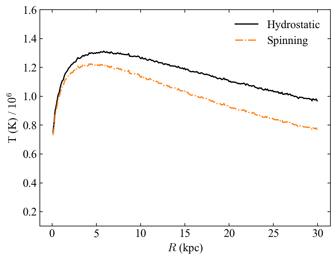
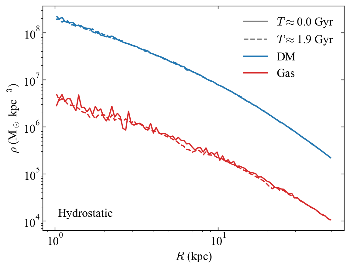
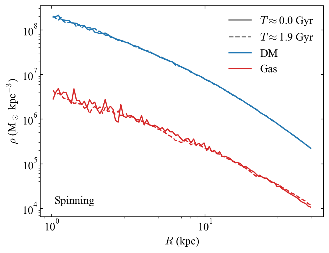
Figure 1: Top: Temperature profile of the hot halo in the hydrostatic case (solid black; Eq. 3) and with spin (dot-dashed orange; Eq. 4). In a state of equilibrium, the temperature of a spinning corona is lower relative to a pure hydrostatic configuration as a result of the additional rotational support against gravity. Middle/Bottom: Volume density profile of the DM halo (blue) and hot gas halo (red) in the hydrostatic case (middle) and the case of a spinning corona (bottom). The solid lines correspond in each case to the initial state of the component, and they are identical across panels. The dashed curve corresponds to the state of the component after roughly $t=1.9$ Gyr of evolution in isolation under adiabatic conditions. Note that the dashed lines, while not identical, are very similar across panels, and also very similar to their corresponding solid curves, attesting the stability of the initial conditions and the robustness of ramses in evolving these.

5.1.1 Hydrostatic, adiabatic halo

Our first test case consists of a hydrostatic, hot halo in thermodynamic equilibrium with the total potential, which follows a temperature profile given by Eq. (3), and shown in the top panel of Fig. 1 by the solid, black curve. Clearly, the halo is not isothermal, but features a temperature on the order of $T\sim 10^{6}$ K – close to the ‘virial temperature’ of the DM halo – with a profile that increases from the centre outwards up to $r\approx 5$ kpc only to decline again.

We evolve the composite system in a cubic box of size 500 kpc per side, adopting a maximum refinement level $l=13$, implying a maximum spatial resolution of 500 kpc / $2^{13}\approx 61$ pc, for roughly 2 Gyr under strict adiabatic conditions. The expectation is that the system maintains its initial state indefinitely.

A departure from equilibrium is not trivial to quantify, but we can put an estimate based on e.g. the evolution of the density structure. We calculate the initial volume density profile of the hot halo and of the DM halo separately, and compare each to the corresponding profile at the end of the simulation. The result of this exercise is displayed in the central panel of Fig. 1. Neither the DM halo (blue curve) nor the hot halo (red curve) display a significant evolution in terms of their mass distribution, as can be seen by comparing their corresponding initial profile (solid curves) with their profile at $t\approx 2$ Gyr (dashed curves). In particular, neither component features a significant change in its central density (generally indicative of the system being out of equilibrium; compare to e.g. Teyssier et al., 2013, their figure 1). The absence of such a change, and the general agreement of the initial and of the evolved profiles, are both strong indications that the system is in a stable, dynamical equilibrium from the outset.

We have made use of this type of halo model extensively in the past (Tepper-García & Bland-Hawthorn, 2018a, b; Tepper-García et al., 2019, see also Mastropietro et al. 2005). However, as mentioned earlier, they are not realistic enough. Yet, the adoption of such models has proven useful as demonstrated by the latter study in particular, which emphasised the importance of the presence of a hot halo component in galaxy models that push towards completeness, as spectacularly demonstrated by Lucchini et al. (2020) and Krishnarao et al. (2022) with the prediction and putative detection, respectively, of the Magellanic Corona.

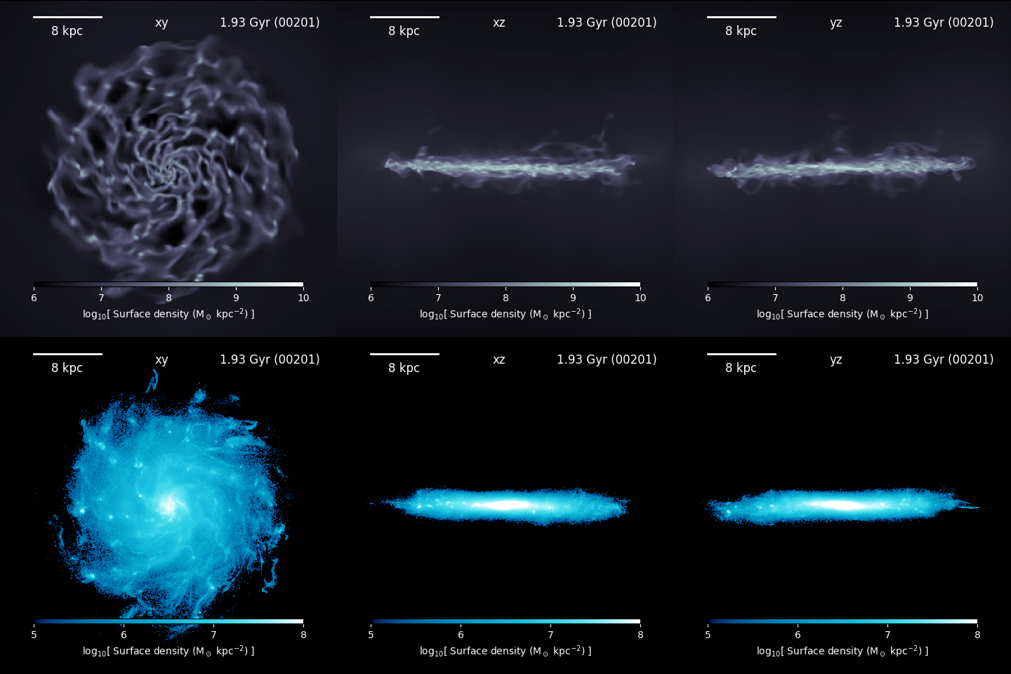
Figure 2: State of a spinning, cooling halo embedded within a responsive DM halo after roughly 2 Gyr of evolution. Top: Gas. Bottom: Newly formed stars

5.1.2 Spinning, adiabatic halo

Our next test setup consists of a non-isothermal, spinning corona, in vertical hydrostatic equilibrium (vHSE). Its temperature profile is shown in the top panel of Fig. 1 by the dot-dashed, orange curve. This mass distribution of this model is identical to the hydrostatic model discussed in Sec. 5.1.1, but their temperature profiles are clearly different as a consequence of the different kinematic structure. Specifically, this spinning model features an overall lower temperature profile, because the rotation velocity provides additional support against gravity (cf. Eq. 4). The velocity has been determined by requiring that the spin parameter of the hot halo be $\lambda=0.12$, consistent with the findings from cosmological simulations (e.g. Agertz & Kravtsov, 2016; Pichon et al., 2011). Note that the DM halo has no net rotation in any of our models (but it is worth emphasising that it can be easily added if so desired within our framework).

As with the hydrostatic model, this model is expected to be in a stable equilibrium from the outset. To check for this, we proceed as we did with the hydrostatic model: we calculate the evolution of the systems over roughly 2 Gyr under adiabatic conditions, and compare the initial and final density profiles of each component (DM halo, hot halo). The result is displayed in the bottom panel of Fig. 1. Overall, the final density profiles of both components agree well with their respective initial profile. Based on this, we are confident that the system is in a stable equilibrium from the outset.

5.1.3 Spinning, cooling halo

The last test within the category of hot halos consists in the classical setup of a spinning, cooling galactic halo pioneered by Kaufmann et al. (2006, see also ), followed by a long list of studies (e.g. Roškar et al., 2008; Teyssier et al., 2013; Hobbs et al., 2013; Marasco et al., 2015; Khoperskov et al., 2021).

The initial conditions are identical to the model discussed in Sec. 5.1.2, but they are advanced in time, allowing the gas to evolve thermodynamically (cool / heat) and to form stars (cf. Sec. 4). In this case, the system will not retain its initial configuration. Rather, the hot gas loses part of its pressure support as a result of cooling, and collapses. Angular momentum conservation deters the gas from collapsing spherically, and collapse proceeds along the spin axis, resulting in a disc-like, rotationally supported gas configuration.

The state of the system after roughly 2 Gyr of evolution is presented in Fig. 2. The top row displays the gas distribution along three orthogonal projections: face-on (left), and side-on (centre/right). The bottom row shows the distribution of newly formed stars along the same projections. The gas disc features a clear spiral-like structure, as well as gas plumes and other gas structures reminiscent of galactic fountains. The disc of newly formed stars is thickened, and displays spiral arm-like features, a number of dense stellar ‘knots’, including a central mass concentration. These results are very much in agreement with the results of similar earlier work (see references above).

This classical setup is indeed a beautiful demonstration of the idea that galaxies may form out of the cooling of shock-heated gas that has been accreted onto DM halos (cf. Sec. 2.1).

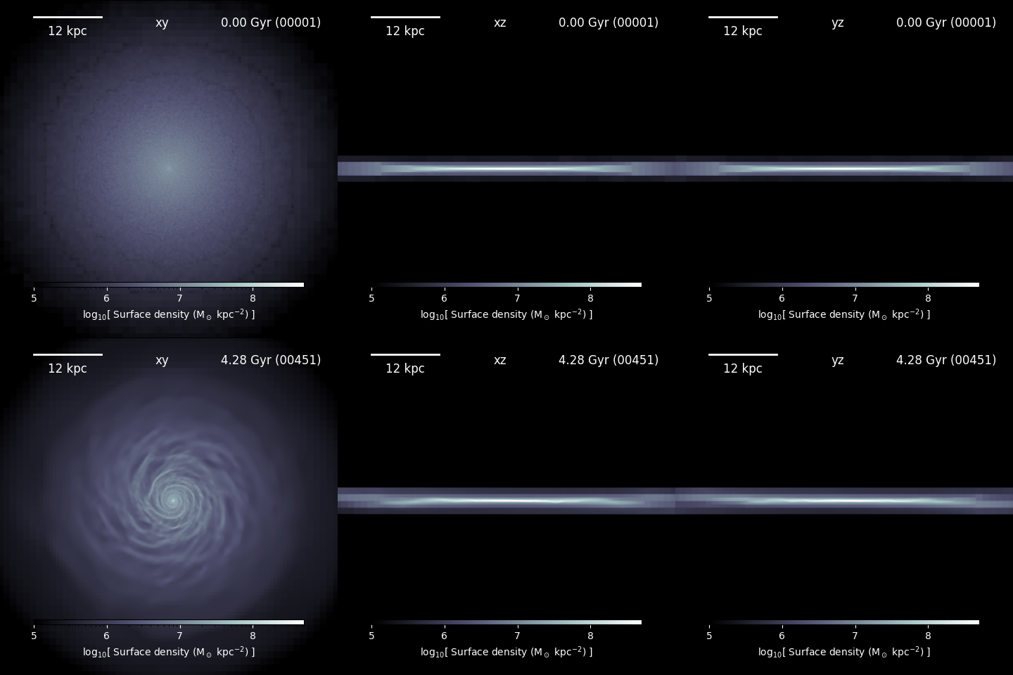
Figure 3: Gas surface density of a strictly isothermal disc embedded within a responsive DM halo - bulge - stellar disc system (not shown). Top: Initial state. Bottom: State after roughly 4.3 Gyr of evolution. Note that the disc develops some sub-structure, clearly visible on the face-on projection (left), as well as a pile-up of mass at the centre (see also Fig. 4), but it retains its overall structure, in particular its thickness (middle, right).

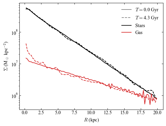
Figure 4: Surface density profile of the stellar disc (black) and gas disc (red) of the simulation test shown in Fig. 3. The solid lines correspond in each case to the initial state of the component. The dashed curve corresponds to the state of the component after roughly $t=4.3$ Gyr of evolution in isolation using an isothermal EoS. Note that the dashed lines, while not identical, are very similar to their corresponding solid curves, attesting the stability of the initial conditions and the robustness of ramses in evolving these. The most notable difference between these two states is the pile-up of gas mass close to the centre (see also Fig. 3).

Table 2: Galaxy model parameters (Sec. 5.2). Columns 1 and 2 identify the galactic components and their associated functional forms; we note that these are approximations because they share the same gravitational potential. The total mass, scale length and cut-off radius are indicated in columns 3, 4, and 5 respectively. Column 6 is the number of particles used to sample the corresponding component. Note that for gaseous components, this number corresponds only to the initial particle number.

Component	Profile	Total mass	Radial scalelength	Cut-off radius	Particle count
		$M_{\rm tot}$	$r_{s}$	$r_{c}$	$N$
		($10^{10}$ M⊙)	(kpc)	(kpc)	($10^{5}$)
DM halo	NFW	145	15	300	20
Stellar bulge	Hernquist	1.5	0.6	2.0	4.5
Stellar disc	Exp, $\operatorname{sech}^{2}$	3.4	3.0	40	10
Gas disc	Exp, $\operatorname{sech}^{2}$	0.4	7.0	–	20

• Notes: The NFW and Hernquist functions are defined elsewhere (Navarro et al., 1997; Hernquist, 1990). The scaleheight of the stellar disc is $z_{t}\approx 250$ pc; the Toomre local instability parameter of the stellar disc is everywhere $Q\gtrsim 1.3$. The gas disc is isothermal with $T=10^{3}$ K, with a scaleheight that varies with radius from roughly 20 pc near the centre to 160 pc at $R=20$ kpc (a ‘flaring’ disc). The gas disc is not truncated, but merges smoothly with the background density (set at $10^{-20}$ cm^-3 in our ramses setup).

5.2 A galaxy with an isothermal gas disc

As a final test of our framework, we set up an isothermal ($T=10^{3}$ K) gas disc embedded in a responsive DM Halo-Bulge-disc (HBD) system, i.e. an isolated galaxy consisting of a DM halo, a classical stellar bulge, a stellar disc and a gaseous disc. This model is virtually identical to the isolated galaxy model underlying one of our earlier studies (Tepper-García et al., 2022), but at a somewhat lower particle resolution. The relevant model parameters are displayed in Tab. 2.

We evolve the composite system in a cubic box of size 600 kpc per side, adopting a maximum refinement level $l=14$, implying a maximum spatial resolution of 600 kpc / $2^{16}\approx 37$ pc, for roughly 4.3 Gyr using a strict isothermal equation of state. Again, we expect the system to retain its initial state, and test this expectation by comparing the initial surface density profile of the stellar disc and of the gas disc to their corresponding profile after 4.3 Gyr of evolution. We do not look at the DM halo and bulge, as we have shown previously that such spheroidal components remain roughly in a stable equilibrium within our framework.

A snapshot of the initial state gas disc and its state at $t\approx 4.3$ Gyr is displayed in the top and bottom panels of Fig. 3, respectively. Although the disc clearly departs from its initially smooth appearance and develops sub-structure, it retains its overall shape, in particular its thickness. This is a clear improvement over the results from similar approaches (compare to e.g. Deg et al., 2019, their figures 1 and 6). The stellar disc displays a similar behaviour (not shown, but see Footnote 24).

A more quantitative assessment of the system’s stability is presented in Fig. 4, which displays the initial surface density profile of the stellar disc (solid black curve) and of the gas disc (solid red curve), and the corresponding profile after roughly 4.3 Gyr of evolution (black and red dashed curves, respectively). The stellar disc shows barely any change with respect to its initial state. The gas disc does show some departure from its initial state, notably a mass pile-up close to the centre and instabilities at the edge. Nonetheless, overall, the system appears to be in a stable equilibrium from the outset. In addition, isothermal setups like this are more of academic interest since they are not realistic when it comes to modelling real galaxies. Once the gas is allowed to evolve thermodynamically, the system will necessarily move away from its initial state, as demonstrated in the next section.

6 A nested-bar system

As a further application of our framework, we extend the model of a barred MW surrogate previously discussed in Tepper-Garcia et al. (2021) to include a gaseous disc component. The relevant model parameters are listed in Tab. 3. The synthetic galaxy consists thus of four components, all of them responsive: a DM host halo, a stellar classical bulge, a stellar disc, and a gas disc. Notably, the disc-to-total mass fraction of the model is $f_{\mathrm{disc}}\approx 0.45$, which renders the disc bar-unstable from the outset (cf. Fujii et al., 2018; Bland-Hawthorn et al., 2023, 2024).

Table 3: Galaxy model parameters (cf. Sec. 6). Meaning of columns and quantities identical to Tab. 2.

Component	Profile	Total mass	Radial scalelength	Cut-off radius	Particle count
		($10^{10}$ M⊙)	(kpc)	(kpc)	($10^{6}$)
DM halo	NFW	118	19	250	1
Stellar bulge	Hernquist	1.25	0.6	2.0	0.1
Stellar disc	Exp, $\operatorname{sech}^{2}$	4.31	2.5	25	1
Gas disc	Exp, $\operatorname{sech}^{2}$	0.46	3.5	–	2

• Notes: The scaleheight of the stellar disc is $z_{t}\approx 300$ pc; the Toomre local instability parameter of the stellar disc is everywhere $Q\gtrsim 1.3$. The gas disc is initially isothermal with $T=10^{3}$ K, with a scaleheight that varies with radius from roughly 20 pc near the centre to 160 pc at $R=20$ kpc (a ‘flaring’ disc). The gas disc is not truncated but merges smoothly with the background density (set at $10^{-20}$ cm^-3 in our ramses setup). The initial gas metallicity is set to 1 Z_⊙ in the disc and zero elsewhere. The initial gas temperature is set to $10^{6}$ K beyond the disc. The disc-to-total mass fraction is $f_{disc}\approx 0.45$, which renders the disc bar-unstable from the outset (cf. Fujii et al., 2018; Bland-Hawthorn et al., 2023).

6.1 Simulation and results

We evolve the initial conditions for roughly 4 Gyr in a cubic volume of 600 kpc across, adopting a maximum spatial resolution of roughly 61 pc. The volume is filled with an additional hot ($T=10^{6}$ K), tenuous ($n<10^{-6}{\>\!{\rm cm}^{-3}}$) gas atmosphere. The self-gravity of all components is taken into account, and the gas is allowed to evolve thermodynamically and to form stars (cf. Sec. 4).

Given the relatively high central gas densities, star formation takes place nearly instantly and vigorously, leading to the formation of a young stellar disc that grows in an inside-out fashion. At the same time, the pre-existent stellar disc succumbs to the bar instability and develops a clear bar-like structure at the centre at $t\lesssim 1$ Gyr.

The young stellar disc follows suit, and develops a bar of its own aligned with the pre-existent stellar bar of roughly the same size. In addition, the young stars spectacularly develop a second, inner bar. Thus, we distinguish between an outer, pre-existent stellar bar, an outer, newly formed stellar bar, and an inner, newly formed stellar bar.

In Fig. 5, we show the state of the pre-existent stellar disc (top row) and of newly formed stellar disc (middle row) after $t=1.9$ Gyr of evolution within a region enclosed by $(x,y)\in[-5,5]\times[-5,5]$ kpc. In each case, the left column displays the projected stellar density; the central column displays the mean projected radial velocity of the stars ($v_{R}$), and the last column displays the projected vertical velocity dispersion of the stars ($\sigma_{z}$).

Focusing on the first row, it is clear that the pre-existent stellar disc has lead to the formation of a central bar with a declining density profile (top-left column), and the classical quadrupole pattern $v_{R}$ (top-middle column), and a vertical velocity dispersion that declines from the centre outwards (top-right column). At the same epoch, the newly formed stellar disc (middle row) also displays a bar-like structure at its centre, which appears aligned with the bar in the pre-existent stellar disc, but is somewhat weaker in terms of density (middle-left column). A notable difference between the pre-existent and the newly formed bars is the presence in the latter of an oblong, central mass concentration with a semi-mayor axis seemingly perpendicular to that of the outer bar. The presence of this inner structure is apparent in the $v_{R}$ map (middle-central column), which displays two quadrupole patterns, one smaller embedded within the more extended one. This is reminiscent of the kinematics observed in a similar system found in cosmological simulations, formed by tidal interaction rather than by an internal instability (Semczuk et al., 2024, their fig. 4).

The vertical velocity dispersion of the newly formed disc (middle-right column) differs significantly from that of the pre-existent stellar disc; notably, it displays two kinematically distinct components: one with a kinematic structure reminiscent of the pre-existent stellar bar, but less extended, which appears to align with the inner bar, superimposed on a more extended structure with a hot kinematic signature along its semi-major axis, aligned with the outer bar. These features are the so-called $\sigma$-‘humps’ and $\sigma$-‘hollows’ previously identified by Du et al. (2016, see also ), and reproduced in some simulations (e.g. Li et al., 2023; Semczuk et al., 2024).

The last row in Fig. 5 displays the state of the system after $t=3.8$ Gyr. A few differences with respect to the state of the newly formed disc some 2 Gyr earlier (middle row) are apparent. First, the central part of the inner bar appears to have collapsed into a bulge by the end of the simulation (bottom-left column). This is interesting because it has been suggested that dissolved inner bars may be the origin of classical bulges (Du et al., 2017). Moreover, the $v_{R}$ map is less well-defined, in particular within the inner bar region, suggesting that the bars may be weakening. Finally, while the $\sigma_{z}$ map displays the same qualitative features (hollows, humps) it suggests that the bars have become kinematically hotter.

We look at the behaviour and structure of the stellar discs throughout the simulation in a holistic way by calculating the evolution of the amplitude of the $m=2$ Fourier mode, $\overline{A}_{2}\equiv A_{2}/A_{0}$ and its phase $\phi[\overline{A}_{2}]$ in space and time (e.g. Mitrašinović & Micic, 2023). In practice, we calculate the radial profile of $\overline{A}_{2}$ within a circular aperture with radius $R=5$ kpc at every time step $T$, effectively yielding a map $\overline{A}_{2}(R,\leavevmode\nobreak\ T)$ and $\phi(R,T)$, respectively, for each of the pre-existent stellar disc and the newly formed stellar disc. The result of this exercise is shown in Fig. 6.

The left panels display $\overline{A}_{2}(R,\leavevmode\nobreak\ T)$ for the pre-existent stellar disc (top) and the newly formed stellar disc (bottom). The formation of a bi-symmetric structure within $R=5$ kpc, signalled by a high value of $\overline{A}_{2}$, is apparent in the pre-existent stellar disc at $t\approx 1$ Gyr, persisting all the way to $t\approx 3.9$ Gyr. The same is true for the newly formed stellar disc. It, however, also displays an inner ($R\lesssim 2$ kpc) signal with a high $\overline{A}_{2}$ amplitude indicative of the presence of an inner bar. Its signal is less consistent than that of the outer bar, and the signal close to the centre weakens at $t\gtrsim 2.7$ Gyr, suggesting the bar is slowly dissolving. This is consistent with the density distribution appearing more centrally concentrated towards the end of the simulation (cf. Fig. 5, bottom-left).

The right panels display $\phi(R,T)$ for each of the pre-existent stellar disc (top) and the newly formed stellar disc (bottom). The former shows an alternating pattern in $\phi$, as expected for a rotating bar, which appears constant all the way to the centre at a given time step, strongly supporting the existence of a well-defined pattern speed of the outer pre-existent bar. This behaviour is mimicked by the newly formed stellar disc. In contrast, there is a second signal, most apparent within $R=1$ kpc, which presumably indicates the pattern speed of the inner bar. It seems to be in lock-step with the outer bar, suggesting their semi-major axes are and remain perpendicular to one another at all times. Note that the signal is fading at $t\gtrsim 2.7$ Gyr, consistent with the weakening of $\overline{A}_{2}$ at the same epoch.

We note the ‘pulsating’ nature of the $\overline{A}_{2}$ amplitude in both disc components, which shows an abrupt change at $t\approx 2.8$ Gyr in both components. Pure visual inspection suggests that its ‘beat’ is different from the phase’s bit, and it is unclear at this point whether they are related and what the origin of the former might be.

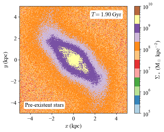
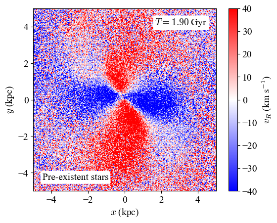
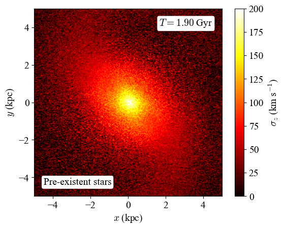
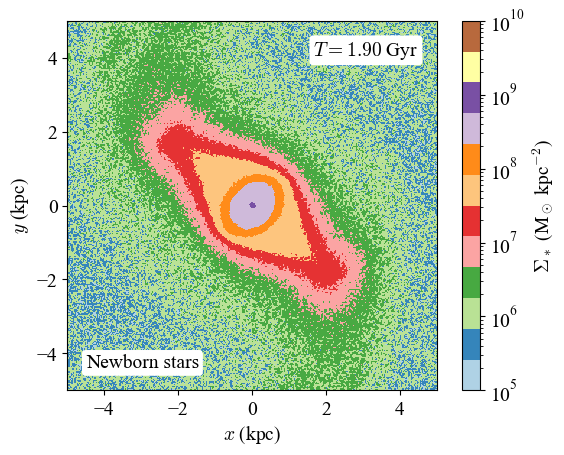
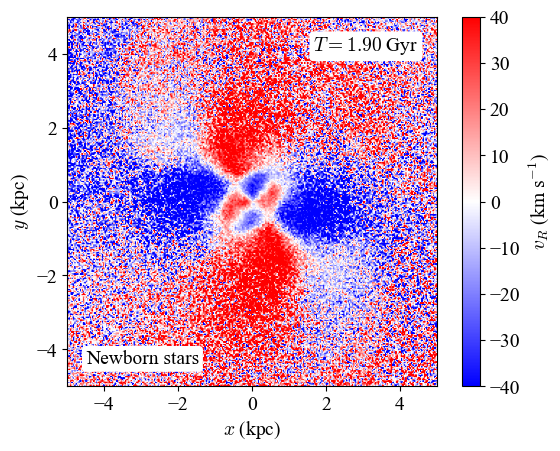
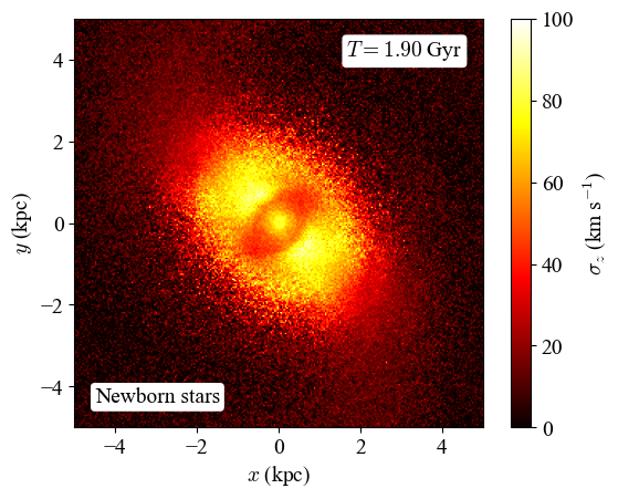
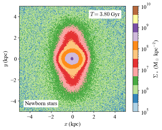
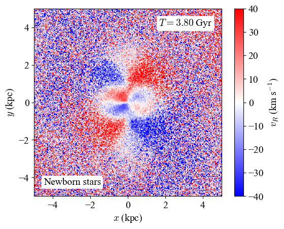
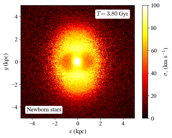
Figure 5: Projected mass density (left), projected radial velocity (centre), and projected vertical velocity dispersion (right) of the pre-existent stars (top), and of the newly formed stars (middle/bottom) after $t\sim 2$ Gyr (top/middle) and $t\sim 4$ Gyr (bottom) of evolution. Note the nested-bar structure in the young stellar component. The outer bar aligns with the bar in the pre-existent stellar component, and precedes the formation of the inner bar (cf. Fig. 8), which appears perpendicular to the outer bar. Notice the difference in scale in the vertical velocity dispersion between the top and the bottom rows, so chosen to avoid colour saturation. The galaxy shows the characteristic kinematic features of nested-bar galaxies: the double quadrupole for mean $v_{R}$ (centre) and humps at the minor axis of the inner bar for $\sigma_{z}$ (right). The central part of the inner bar appears to have collapsed into a bulge by the end of the simulation.

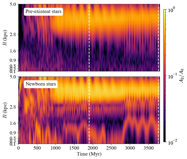
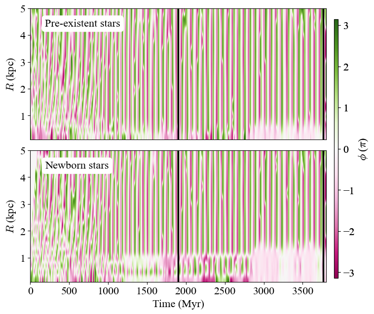
Figure 6: Evolution of the $m=2$ Fourier amplitude ($A_{2}/A_{0}$; left) and its phase ($\phi$; right) across the bar region ($R\leq 5$ kpc) over a period of roughly 3.8 Gyr for each stellar component separately. Top: Pre-existent stars. Bottom: Newly formed stars. Note that the radial range is equally spaced on a logarithmic scale on the left panels, but on a linear scale in the right panels. The bottom panel displays a clear strong signal (i.e. a high $A_{2}/A_{0}$ value as indicated by the colour-bar on the right) both within $0<R/{\>\!{\rm kpc}}\lesssim 2$ and $3\lesssim R/{\>\!{\rm kpc}}<5$, indicating the presence of an inner and of an outer bar, respectively. The top panel indicates the presence of an outer bar only. The inner bar phase appears in lock-step with the outer bar, suggesting they remain perpendicular at all times. Note that all bars persist out to at least $t\sim 2.7$ Gyr, after which it seems to lead to the formation of a central mass concentration (likely a classical bulge). The vertical, dashed lines flag the epoch corresponding to the snapshots underlying Figs. 5 and 8.

Given the putative connection between the presence of nested bars in galaxies and the fuelling of active galactic nuclei (AGN) and black-hole growth (Shlosman et al., 1989; Namekata et al., 2009; Du et al., 2017), it is interesting to look now at the gas flow in and around the galaxy centre. To this end, we proceed as follows. First, we calculate the enclosed mass within two circular apertures with radii $R=5$ kpc and $R=2$ kpc, roughly enclosing the outer bars and the inner bar. We separately look at the enclosed gas mass and the mass of newly formed stars, as well as at their combined mass (since stars form from gas). The latter approach allows assessing the mass change within the respective bar regions. To gain some insight into the mass flow, we calculate the time derivative of the enclosed mass profile, following Li et al. (2023).

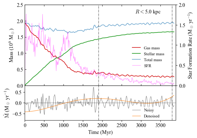
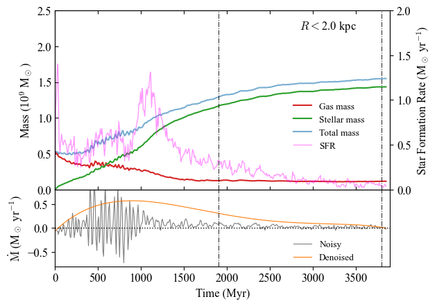
Figure 7: Evolution of the mass (gaseous, stellar, and total, i.e. gaseous and stellar added together) enclosed within two circular apertures: $R<5$ kpc (left) and $R<2$ kpc (right). The total star-formation rate within each of these regions is shown as well (scale is provided on the right $y$-axis and is identical in both panels). The sub-panel at the bottom displays in each case the total mass flow rate, estimated from the derivative with respect to time of the total enclosed mass (see text for details). The vertical, dot-dashed lines flag the epoch corresponding to the snapshots underlying Figs. 5 and 8.

The result is presented in Fig. 7. The main panels display the gas (red curve), stellar (green curve) and total (gas plus stellar; blue curve) mass enclosed within two circular apertures around the centre with radius $R=2$ kpc (left) and 5 kpc (right). The sub-panels in each case display the total mass flow rate, $\dot{M}$ (in units of M_⊙ yr ^-1 ) estimated from the derivative with respect to time of the total enclosed mass. The derivative is calculated both on the total enclosed mass data as is (termed ‘noisy’; grey curve) and a ‘de-noised’ version of it (orange curve). The latter is calculated by interpolating the noisy data with a spline function. The reason is that the derivative of the noisy data may provide information on the periodicity of the mass flow, while the derivative of the de-noised data better estimates the actual net mass flow.

We find that the inner region, which encloses the inner bar, experiences a net mass inflow, while the outer region – which encloses the outer bar – displays a rather flat mass growth on average. This behaviour can be understood by looking at the star-formation rate (SFR) averaged over the aperture, shown by the magenta curve, in each case. Within the larger region (right panel), we observe a clear correlation between enhanced SFR, gas depletion (red), and stellar mass growth (blue) over a period of $t\approx 1.5$ Gyr since the start of the simulation. Overall, the gas depletion dominates over stellar mass growth ($\dot{M}<0$, orange curve) during that time, suggesting that some of the gas is lost to outflows as a result of the vigorous stellar activity. As the latter starts fading, the gas consumption levels off, as does the growth of new stellar mass, and the total mass within the region climbs up to roughly the level it had initially.

The behaviour is somewhat different within the smaller region ($R<2$ kpc). After an initial, nearly instantaneous star-formation burst, the SFR drops dramatically and maintains roughly the same level out to $t\approx 1$ Gyr, at which point it increases significantly. There is a clear net gas mass inflow into the region ($\dot{M}>0$, orange curve), that may in fact lead to the formation of the inner bar.

In either region, the mass flow rate appears quasi-periodic (see sub-panels; grey curves), in agreement with Li et al. (2023), presumably as a result of the bar’s rotation (cf. Fig. 6, right). A full Fourier analysis of the mass inflow to confirm or reject this suspicion is well beyond the scope of this paper and is therefore left for future work.

The delayed mass flow into the inner region suggests that the stars formed there should, on average, be younger compared to the average population of the outer region. In addition, given that the gas is flowing from the outer region and has likely to be enriched by earlier generations of stars, the mean metallicity of the stars within the inner region should, on average, be higher compared to the stars in the outer region.

In Fig. 8 we display at two different epochs, $t=1.9$ Gyr and $t=3.9$ Gyr, the mean projected stellar age (left), the mean projected stellar metallicity (middle), and the star-formation rate density (in a time period of 500 Myr relative to the given epoch) within a region enclosed by $(x,y)\in[-5,5]\times[-5,5]$ kpc.

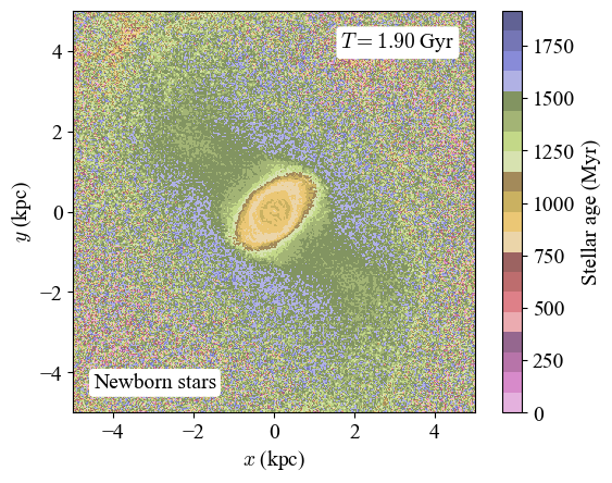
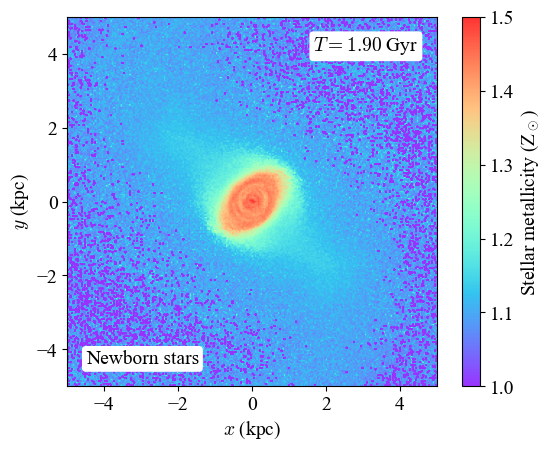
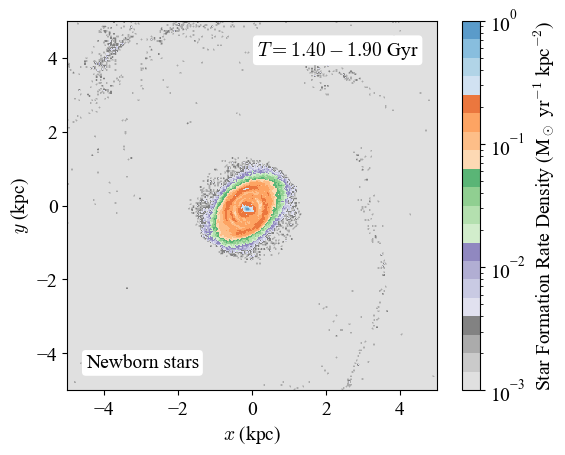
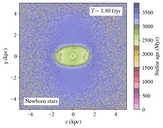
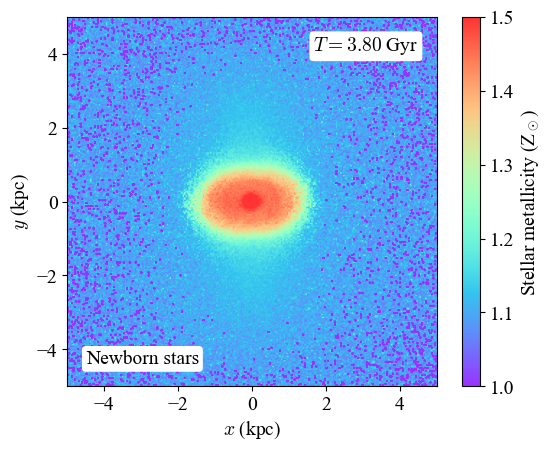
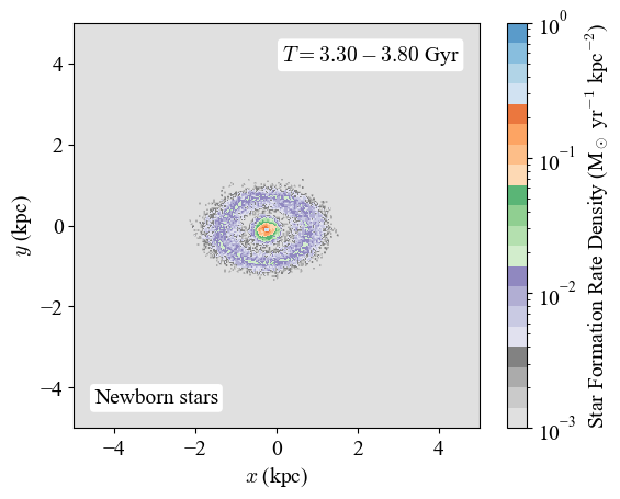
Figure 8: Mean stellar age (left), mean stellar metallicity (middle), and star-formation-rate density (SFRd; right) within the bar region ($R\leq 5$ kpc) after $t\approx 1.9$ Gyr (top) and 3.8 Gyr (bottom) of evolution. Note that the SFRd is calculated taking into account all the stars born in the last 500 Myr with respect to the given epoch. Clearly, the inner bar is younger compared to the outer bar at all times, but their ages both increase with time (note the difference in the colour range between the middle and the bottom panels). Note that the inner bar is more apparent here than it is in terms of its density distribution (Fig. 5), where it appears to have collapsed into a more circular mass concentration by the end of the simulation. Star formation is virtually only taking place within the inner bar region and decreasing rapidly with time, as can be seen by comparing the top and bottom panels in the last column.

As suspected, we find that the stellar population of the inner bar is younger on average than that of the outer bar, implying that the inner bar forms after the outer bar, in agreement with Wozniak (2015). Interestingly, this behaviour of bars formed due to an internal instability is the diametrically opposed behaviour to what is observed in the case where the bar formation is tidally induced (Semczuk et al., 2024). Star formation is virtually only taking place within the inner bar region and decreasing rapidly with time, as can be seen by comparing the top and bottom panels in the last column, consistent with the results displayed in Fig. 7 (magenta curve).

Semczuk et al. (2024, see also ) note that in the case of NGC 1291, star formation can still happen outside the inner bar, after this was formed, and therefore ages of the inner bar can be still older than its surroundings. This is apparent in the top panel of Fig. 8, where an older (brown colour) nuclear stellar ring is surrounded by a younger structure (gold colour). The age distribution is mirrored by a metallicity distribution, as perhaps anticipated: younger stars are on average more enriched and the more enriched stars occupy the regions closer to the centre. The presence of an older ring is also apparent in the metallicity map, visible as ring-like structure with a metallicity which is on average lower compared to its surroundings.

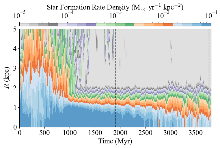
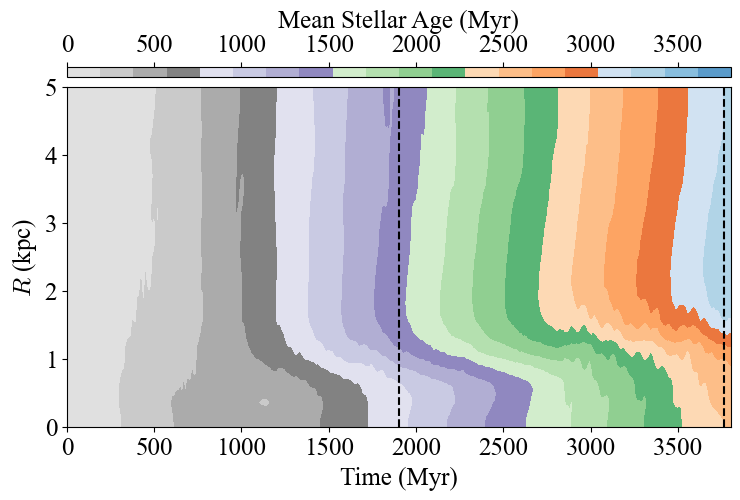
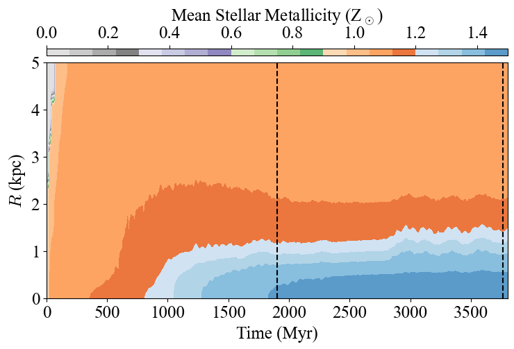
Figure 9: Top: Star-formation rate density within the bar region ($R<5$ kpc). Middle: Stellar age. Bottom: Stellar metallicity. Although not always a good practice, in this case we consciously adopt the same colour scheme across all three panels to emphasise the connection between SFR on the one hand, and stellar age and stellar metallicity on the other. The vertical, dashed lines flag the epoch corresponding to the snapshots underlying Figs. 5 and 8.

A holistic view of the causal connection between SFR, stellar age and their enrichment is provided in Fig, 9. It displays the evolution in space and time of the star-formation rate density (in units of (M_⊙ yr^-1 kpc^-2); top), the mean stellar age (in Myr; middle), and the mean stellar metallicity (in solar units; bottom).

It is apparent that the star-formation rate density decreases radially outwards at any given time, and also decreases with time at any given radius. Correspondingly, he mean stellar age at a given radius increases with time, and at any given time the mean stellar age decreases radially outwards. There is a clear trend separating younger from older populations at $R\approx 1$ kpc, i.e. between the inner and the outer bar regions, consistent with the age and metallicity distribution at the specific snapshots displayed in Fig. 8.

6.2 Discussion

Nested-bar systems (historically referred to as ‘double-barred’ or S2B for short) have been known since de Vaucouleurs (1975); Sandage & Brucato (1979), and they have been studied in some detail both in observations (e.g Moiseev, 2001; Erwin, 2004) and simulations (e.g Debattista & Shen, 2007; Wozniak, 2015). It has been suggested that even the MW may feature a nested bar (Alard, 2001; Namekata et al., 2009). Roughly 20 percent of barred galaxies in the Local Universe feature a second, inner bar, and the frequency of S2B systems increases with stellar mass (Erwin, 2024).

This type of system is not only interesting because of its exotic nature, but it is also of high relevance in the context of black-hole (BH) growth and active galactic nuclei (AGN) fuelling (Shlosman et al., 1989, 1990). The basic idea is that the inner bar promotes the inflow of gas towards the centre beyond the radius that the outer bar usually does. It also has been suggested based on theoretical work that, if short-lived, dissolved inner bars may be the origin of bulges (e.g. Du et al., 2017).

The simulation presented here appears to support both of these beliefs. Indeed, the system undergoes a significant gas mass inflow towards the centre leading to an enhanced star formation, a younger and more enriched stellar population, compared to the surroundings. But the inner bar does not seem to be long-lived, i.e. over $t\gtrsim 1$ Gyr, and rather appears to dissolve, yielding to the formation of a pseudo-spherical mass concentration (‘bulge’), Whether this behaviour and the absence of a central black hole in the galaxy is related to a numerical aspect of our simulation such as the limited spatial resolution, or to a physical one such as the strength of the stellar feedback, is unclear at the moment.

Our simulation features both interesting similarities and differences with respect to earlier, similar simulations. For instance, the synthetic galaxy is bar unstable because it is baryon-dominated in the inner region (Fujii et al., 2018; Bland-Hawthorn et al., 2023). This is in stark contrast to Saha & Maciejewski (2013), who find that a dominant halo and a hot disc and no gas are needed for the system to spontaneously form a nested-bar structure. In comparison to Semczuk et al. (2024), in our simulation, the inner stellar bar appears perpendicular to the outer bar at nearly all times. The latter may be explained by the fact that the nested-bar nature of the galaxy in our simulation and Semczuk et al. (2024)’s forms through diametrically different channels: in their case, it is tidally (i.e. externally) triggered, while in our simulation it is internally triggered. In their case, the outer bar forms after the inner bar. Interestingly, both simulated galaxies show the characteristic kinematic features of nested bars: the double quadrupole for mean $v_{R}$ and humps at the minor axis of the inner bar for $\sigma_{z}$ (see also de Lorenzo-Cáceres et al., 2008).

A notable difference with respect to earlier examples of barred galaxies is that the galaxy in our simulation displays what could be considered to be three independent bar components, which motivates us to define it as a new class of model, i.e. a triple-barred (S3B) galaxy. We are not aware of any previous report of a triple-barred system in either observations or simulations. If such systems do exist, we speculate that a possible formation channel would be the case of a barred disc galaxy with an old disc component that experiences accretion of a significant mass of gas, from which a new disc component forms. This, however, is purely speculative and more work is needed to understand the detailed properties of systems like this, beginning with its frequency.

7 Concluding Remarks: The case for controlled experiments

Controlled experiments of idealised galaxies sit between theoretical models and cosmological simulations, and are complementary to both. They are very useful for isolating processes that are not easily apparent in a cosmological setting. The advantage of a controlled experiment is especially apparent when dealing with highly non-linear processes. Cosmological simulations have the advantage of treating the evolving hierarchy realistically, since mass assembly is largely driven by the dark matter. Once baryons are included, it becomes increasingly difficult to understand the role of interacting processes given the very large number of free parameters, made more difficult by inadequate numerical resolution. In general, the best results have come from re-running a simulation of a specific “local volume” at higher resolution (e.g. Sorce et al., 2016; Ma et al., 2017) but even then, there are many competing processes to unwind.

Famously, some of the earliest (restricted) N-body calculations (Toomre & Toomre, 1972) revealed the emergence of bridges, tails and spiral-like features in galaxy-galaxy interactions. Related phenomena include stellar shells interleaved in radius that are due to an infalling satellite (Quinn, 1984; Barnes & Hernquist, 1992), now detected in cosmological simulations (Pop et al., 2018). In a seminal paper, through controlled simulations, Sellwood & Carlberg (1984) showed how spiral instabilities are triggered by accretion and star formation, and are likely to be transient features of disc galaxies.

There are numerous examples of how controlled N-body experiments have led to new insights in galactic dynamics (Athanassoula, 1992). Typically, these manifestations are preceded by a strong theoretical basis, but not always (Binney & Tremaine, 2008). The discovery of two-dimensional (2D; Hohl, 1971) and three-dimensional (3D; Combes et al., 1990) bar instabilities came from early N-body simulations of isolated discs. Later, it was shown that bars must slow down due to the exchange of energy through dynamical friction with a responsive dark matter halo (Debattista & Sellwood, 1998). A related process also makes a difference to the accretion of satellites in low-eccentricity orbits, and dynamical friction of these systems against the baryon disc can be much more important than against the dark halo (Walker et al., 1996).

After Sellwood & Binney (2002) argued on theoretical grounds that stellar migration was possible, Roškar et al. (2008) realised the same behaviour in an isolated N-body disc, albeit with much higher rates of migration. Inner and outer disc rings and resonances (Sellwood & Wilkinson, 1993), outer disc warps and flares (Binney, 1992; Reshetnikov & Combes, 1998) were first realised in controlled N-body experiments, as were other manifestations like disc heating due to disc-crossing satellites (Quinn et al., 1993). Some of these early experiments used rigid systems that did not conserve momentum and tended to exaggerate the energy exchange. Fully N-body experiments with live dark-matter halos established that the disc heating efficiency needs to be reduced by an order of magnitude (Hopkins et al., 2008).

Controlled experiments continue to reveal new phenomena up to the present time. When Antoja et al. (2018) discovered the remarkable “phase spiral" in the local disc, this was soon realised in a dozen controlled experiments (e.g. Laporte et al., 2019; Khoperskov et al., 2019; Bland-Hawthorn & Tepper-García, 2021; Hunt et al., 2021) before being detected in cosmological simulations (q.v. García-Conde et al., 2022). Aumer et al. (2016) showed that the observed 3D stellar kinematic dispersions in the Milky Way result largely from the collective effects of scattering in both molecular clouds and spiral arms over cosmic time (c.f. Ida et al., 1993). Impressively, these processes are beginning to emerge in the best zoom-in simulations (McCluskey et al., 2024). When a strong impulse (e.g. disc-crossing massive satellite) warps the outer disc, this triggers a bending wave (corrugation) across the inner disc that wraps up with the disc’s differential rotation (Bland-Hawthorn & Tepper-García, 2021). Beyond the Milky Way, corrugations have since been seen in several disc galaxies with outer warps (Urrejola-Mora et al., 2022).

We recognise that upcoming cosmological simulations will find ways to manufacture realistic gas-rich discs at very early times ($z\gtrsim 6$). This is likely to be a very complex and messy process. Yet, synthetic galaxies at any epoch will continue to be highly idealised in the sense that no method is yet able to fully accommodate magneto-hydrodynamical (MHD) dynamos (e.g. Brandenburg & Subramanian, 2005; Federrath, 2016) and diffusion, supra-thermal particle and cosmic ray heating, dust and molecular processes, and so forth. In part, our motivation for the new work is to provide a framework for simplifying what is seen in cosmological simulations with a view to understanding what happens with each added parameter. For instance, our new framework is the ideal setting to understand the long-term relationship between the evolving ISM (governed mainly by the initial gas fraction) and stellar dynamical processes.

In addition to the expansion of our framework’s capabilities in terms of the available halo models, as well as a more refined treatment of the gas chemistry, in upcoming work, we aim to couple our framework to the earliest disc systems emerging in the vintergatan simulations that use, by design, the same star formation and feedback prescriptions (Agertz et al., 2021). The ultimate goal is to create idealised analogues of galaxies that develop within a full cosmological context that can be run under controlled conditions.

References

- Agertz & Kravtsov (2015) Agertz O., Kravtsov A. V., 2015, ApJ, 804, 18
- Agertz & Kravtsov (2016) Agertz O., Kravtsov A. V., 2016, ApJ, 824, 79
- Agertz et al. (2009a) Agertz O., Lake G., Teyssier R., Moore B., Mayer L., Romeo A. B., 2009a, MNRAS, 392, 294
- Agertz et al. (2009b) Agertz O., Teyssier R., Moore B., 2009b, MNRAS, 397, L64
- Agertz et al. (2013) Agertz O., Kravtsov A. V., Leitner S. N., Gnedin N. Y., 2013, ApJ, 770, 25
- Agertz et al. (2015) Agertz O., Romeo A. B., Grisdale K., 2015, MNRAS, 449, 2156
- Agertz et al. (2021) Agertz O., et al., 2021, MNRAS, 503, 5826
- Alard (2001) Alard C., 2001, A&A, 379, L44
- Anderson et al. (2022) Anderson S. R., Debattista V. P., Erwin P., Liddicott D. J., Deg N., Beraldo e Silva L., 2022, MNRAS, 513, 1642
- Andersson et al. (2023) Andersson E. P., Agertz O., Renaud F., Teyssier R., 2023, MNRAS, 521, 2196
- Annem & Khoperskov (2024) Annem B., Khoperskov S., 2024, MNRAS, 527, 2426
- Antoja et al. (2018) Antoja T., et al., 2018, Nature, 561, 360
- Ascasibar et al. (2003) Ascasibar Y., Yepes G., Müller V., Gottlöber S., 2003, MNRAS, 346, 731
- Asplund et al. (2009) Asplund M., Grevesse N., Sauval A. J., Scott P., 2009, ARA&A, 47, 481
- Athanassoula (1992) Athanassoula E., 1992, MNRAS, 259, 345
- Aubert & Teyssier (2010) Aubert D., Teyssier R., 2010, ApJ, 724, 244
- Aumer et al. (2010) Aumer M., Burkert A., Johansson P. H., Genzel R., 2010, ApJ, 719, 1230
- Aumer et al. (2016) Aumer M., Binney J., Schönrich R., 2016, MNRAS, 462, 1697
- Barbani et al. (2023) Barbani F., Pascale R., Marinacci F., Sales L. V., Vogelsberger M., Torrey P., Li H., 2023, MNRAS, 524, 4091
- Barnabè et al. (2006) Barnabè M., Ciotti L., Fraternali F., Sancisi R., 2006, A&A, 446, 61
- Barnes & Hernquist (1992) Barnes J. E., Hernquist L., 1992, ARA&A, 30, 705
- Binney (1977) Binney J., 1977, MNRAS, 181, 735
- Binney (1992) Binney J., 1992, ARA&A, 30, 51
- Binney (2012) Binney J., 2012, Monthly Notices of the Royal Astronomical Society, 426, 1324
- Binney & Tremaine (2008) Binney J., Tremaine S., 2008, Galactic Dynamics: (Second Edition). Princeton Series in Astrophysics, Princeton University Press
- Bland-Hawthorn & Tepper-García (2021) Bland-Hawthorn J., Tepper-García T., 2021, MNRAS, 504, 3168
- Bland-Hawthorn et al. (2023) Bland-Hawthorn J., Tepper-Garcia T., Agertz O., Freeman K., 2023, ApJ, 947, 80
- Bland-Hawthorn et al. (2024) Bland-Hawthorn J., Tepper-Garcia T., Agertz O., Federrath C., 2024, arXiv e-prints, p. arXiv:2402.06060
- Booth et al. (2013) Booth C. M., Agertz O., Kravtsov A. V., Gnedin N. Y., 2013, ApJ, 777, L16
- Brandenburg & Subramanian (2005) Brandenburg A., Subramanian K., 2005, Phys. Rep., 417, 1
- Bregman et al. (2018) Bregman J. N., Anderson M. E., Miller M. J., Hodges-Kluck E., Dai X., Li J.-T., Li Y., Qu Z., 2018, ApJ, 862, 3
- Bullock et al. (2001) Bullock J. S., Dekel A., Kolatt T. S., Kravtsov A. V., Klypin A. A., Porciani C., Primack J. R., 2001, ApJ, 555, 240
- Canivete Cuissa & Teyssier (2022) Canivete Cuissa J. R., Teyssier R., 2022, A&A, 664, A24
- Chabrier (2003) Chabrier G., 2003, ApJ, 586, L133
- Clarke et al. (2019) Clarke A. J., et al., 2019, MNRAS, 484, 3476
- Combes et al. (1990) Combes F., Debbasch F., Friedli D., Pfenniger D., 1990, A&A, 233, 82
- Cuddeford (1991) Cuddeford P., 1991, MNRAS, 253, 414
- D’Ercole & Brighenti (1999) D’Ercole A., Brighenti F., 1999, MNRAS, 309, 941
- D’Onghia & L. Aguerri (2020) D’Onghia E., L. Aguerri J. A., 2020, ApJ, 890, 117
- D’Onghia et al. (2013) D’Onghia E., Vogelsberger M., Hernquist L., 2013, ApJ, 766, 34
- Debattista & Sellwood (1998) Debattista V. P., Sellwood J. A., 1998, ApJ, 493, L5
- Debattista & Shen (2007) Debattista V. P., Shen J., 2007, ApJ, 654, L127
- Deg et al. (2019) Deg N., Widrow L. M., Randriamampandry T., Carignan C., 2019, MNRAS, 486, 5391
- Di Matteo et al. (2005) Di Matteo T., Springel V., Hernquist L., 2005, in A. Merloni, S. Nayakshin, & R. A. Sunyaev ed., Growing Black Holes: Accretion in a Cosmological Context. pp 340–345, doi:10.1007/11403913_65
- Dolag et al. (2017) Dolag K., Mevius E., Remus R.-S., 2017, Galaxies, 5, 35
- Du et al. (2016) Du M., Debattista V. P., Shen J., Cappellari M., 2016, ApJ, 828, 14
- Du et al. (2017) Du M., Debattista V. P., Shen J., Ho L. C., Erwin P., 2017, ApJ, 844, L15
- Dubois & Commerçon (2016) Dubois Y., Commerçon B., 2016, A&A, 585, A138
- Dubois et al. (2016) Dubois Y., Peirani S., Pichon C., Devriendt J., Gavazzi R., Welker C., Volonteri M., 2016, MNRAS, 463, 3948
- Efstathiou & Jones (1979) Efstathiou G., Jones B. J. T., 1979, MNRAS, 186, 133
- Erwin (2004) Erwin P., 2004, A&A, 415, 941
- Erwin (2024) Erwin P., 2024, MNRAS, 528, 3613
- Fall & Efstathiou (1980) Fall S. M., Efstathiou G., 1980, MNRAS, 193, 189
- Federrath (2016) Federrath C., 2016, Journal of Plasma Physics, 82, 535820601
- Federrath & Klessen (2012) Federrath C., Klessen R. S., 2012, ApJ, 761, 156
- Fromang et al. (2006) Fromang S., Hennebelle P., Teyssier R., 2006, A&A, 457, 371
- Fujii et al. (2018) Fujii M. S., Bédorf J., Baba J., Portegies Zwart S., 2018, MNRAS, 477, 1451
- Fukugita & Peebles (2006) Fukugita M., Peebles P. J. E., 2006, ApJ, 639, 590
- García-Conde et al. (2022) García-Conde B., Roca-Fàbrega S., Antoja T., Ramos P., Valenzuela O., 2022, MNRAS, 510, 154
- Girichidis et al. (2018) Girichidis P., Naab T., Hanasz M., Walch S., 2018, MNRAS, 479, 3042
- Grand et al. (2017) Grand R. J. J., et al., 2017, MNRAS, 467, 179
- Grisdale et al. (2017) Grisdale K., Agertz O., Romeo A. B., Renaud F., Read J. I., 2017, MNRAS, 466, 1093
- Grisdale et al. (2018) Grisdale K., Agertz O., Renaud F., Romeo A. B., 2018, MNRAS, 479, 3167
- Grønnow et al. (2018) Grønnow A., Tepper-García T., Bland-Hawthorn J., 2018, ApJ, 865, 64
- Haardt & Madau (1996) Haardt F., Madau P., 1996, ApJ, 461, 20
- Hernquist (1990) Hernquist L., 1990, ApJ, 356, 359
- Hernquist (1993) Hernquist L., 1993, ApJS, 86, 389
- Hobbs et al. (2013) Hobbs A., Read J., Power C., Cole D., 2013, MNRAS, 434, 1849
- Hodges-Kluck et al. (2018) Hodges-Kluck E. J., Bregman J. N., Li J.-t., 2018, ApJ, 866, 126
- Hohl (1971) Hohl F., 1971, ApJ, 168, 343
- Hopkins et al. (2008) Hopkins P. F., Hernquist L., Cox T. J., Younger J. D., Besla G., 2008, ApJ, 688, 757
- Hopkins et al. (2011) Hopkins P. F., Quataert E., Murray N., 2011, MNRAS, 417, 950
- Hopkins et al. (2014) Hopkins P. F., Kereš D., Oñorbe J., Faucher-Giguère C.-A., Quataert E., Murray N., Bullock J. S., 2014, MNRAS, 445, 581
- Hopkins et al. (2018) Hopkins P. F., et al., 2018, MNRAS, 480, 800
- Hopkins et al. (2020) Hopkins P. F., et al., 2020, MNRAS, 492, 3465
- Hoyle et al. (1949) Hoyle F., Burgers J., van De Hulst H., 1949, Central Air Documents Office, Dayton, OH, p. 195
- Hunt et al. (2021) Hunt J. A. S., Stelea I. A., Johnston K. V., Gandhi S. S., Laporte C. F. P., Bédorf J., 2021, MNRAS, 508, 1459
- Hunter (2007) Hunter J. D., 2007, Computing in Science & Engineering, 9, 90
- Ida et al. (1993) Ida S., Kokubo E., Makino J., 1993, MNRAS, 263, 875
- Jeans (1915) Jeans J. H., 1915, MNRAS, 76, 70
- Jubelgas et al. (2008) Jubelgas M., Springel V., Enßlin T., Pfrommer C., 2008, A&A, 481, 33
- Kalberla & Kerp (2009) Kalberla P. M. W., Kerp J., 2009, ARA&A, 47, 27
- Käppeli & Mishra (2016) Käppeli R., Mishra S., 2016, A&A, 587, A94
- Kaufmann et al. (2006) Kaufmann T., Mayer L., Wadsley J., Stadel J., Moore B., 2006, MNRAS, 370, 1612
- Khoperskov et al. (2019) Khoperskov S., Di Matteo P., Gerhard O., Katz D., Haywood M., Combes F., Berczik P., Gomez A., 2019, A&A, 622, L6
- Khoperskov et al. (2021) Khoperskov S., Haywood M., Snaith O., Di Matteo P., Lehnert M., Vasiliev E., Naroenkov S., Berczik P., 2021, MNRAS, 501, 5176
- Kim & Ostriker (2015) Kim C.-G., Ostriker E. C., 2015, ApJ, 802, 99
- Kim et al. (2014) Kim J.-h., et al., 2014, ApJS, 210, 14
- Krause (2019) Krause G., 2019, A&A, 631, A68
- Krishnarao et al. (2022) Krishnarao D., et al., 2022, Nature, 609, 915
- Laporte et al. (2019) Laporte C. F. P., Minchev I., Johnston K. V., Gómez F. A., 2019, MNRAS, 485, 3134
- Lebovitz (1967) Lebovitz N. R., 1967, Annual Review of Astronomy and Astrophysics, 5, 465
- Lehner et al. (2017) Lehner N., Howk J. C., Wakker B. P., 2017, ApJ, 848, 71
- Leitherer et al. (1999) Leitherer C., et al., 1999, ApJS, 123, 3
- Leroy et al. (2009) Leroy A. K., et al., 2009, AJ, 137, 4670
- Li et al. (2023) Li Z., et al., 2023, ApJ, 958, 77
- Lucchini et al. (2020) Lucchini S., D’Onghia E., Fox A. J., Bustard C., Bland-Hawthorn J., Zweibel E., 2020, Nature, 585, 203
- Ma et al. (2017) Ma X., Hopkins P. F., Wetzel A. R., Kirby E. N., Anglés-Alcázar D., Faucher-Giguère C.-A., Kereš D., Quataert E., 2017, MNRAS, 467, 2430
- Marasco et al. (2015) Marasco A., Debattista V. P., Fraternali F., van der Hulst T., Wadsley J., Quinn T., Roškar R., 2015, MNRAS, 451, 4223
- Marinacci et al. (2010) Marinacci F., Binney J., Fraternali F., Nipoti C., Ciotti L., Londrillo P., 2010, MNRAS, 404, 1464
- Mastropietro et al. (2005) Mastropietro C., Moore B., Mayer L., Wadsley J., Stadel J., 2005, MNRAS, 363, 509
- McCluskey et al. (2024) McCluskey F., Wetzel A., Loebman S. R., Moreno J., Faucher-Giguère C.-A., Hopkins P. F., 2024, MNRAS, 527, 6926
- Miller et al. (2016) Miller M. J., Hodges-Kluck E. J., Bregman J. N., 2016, ApJ, 818, 112
- Mitrašinović & Micic (2023) Mitrašinović A., Micic M., 2023, PASA, 40, e024
- Mo et al. (1998) Mo H. J., Mao S., White S. D. M., 1998, MNRAS, 295, 319
- Moiseev (2001) Moiseev A. V., 2001, Bulletin of the Special Astrophysics Observatory, 51, 140
- Naab & Ostriker (2017) Naab T., Ostriker J. P., 2017, ARA&A, 55, 59
- Namekata et al. (2009) Namekata D., Habe A., Matsui H., Saitoh T. R., 2009, The Astrophysical Journal, 691, 1525
- Navarro et al. (1997) Navarro J. F., Frenk C. S., White S. D. M., 1997, ApJ, 490, 493
- Noguchi (1999) Noguchi M., 1999, ApJ, 514, 77
- Nuza et al. (2014) Nuza S. E., Parisi F., Scannapieco C., Richter P., Gottlöber S., Steinmetz M., 2014, MNRAS, 441, 2593
- Oppenheimer (2018) Oppenheimer B. D., 2018, MNRAS, 480, 2963
- Pakmor et al. (2016) Pakmor R., Pfrommer C., Simpson C. M., Springel V., 2016, ApJ, 824, L30
- Peebles (1969) Peebles P. J. E., 1969, ApJ, 155, 393
- Perret (2016) Perret V., 2016, DICE: Disk Initial Conditions Environment, Astrophysics Source Code Library (ascl:1607.002), http://ascl.net/1607.002
- Perret et al. (2014) Perret V., Renaud F., Epinat B., Amram P., Bournaud F., Contini T., Teyssier R., Lambert J.-C., 2014, A&A, 562, A1
- Pezzulli et al. (2017) Pezzulli G., Fraternali F., Binney J., 2017, MNRAS, 467, 311
- Pfrommer et al. (2017) Pfrommer C., Pakmor R., Schaal K., Simpson C. M., Springel V., 2017, MNRAS, 465, 4500
- Pichon et al. (2011) Pichon C., Pogosyan D., Kimm T., Slyz A., Devriendt J., Dubois Y., 2011, MNRAS, 418, 2493
- Pillepich et al. (2018) Pillepich A., et al., 2018, MNRAS, 473, 4077
- Pontzen et al. (2013) Pontzen A., Roškar R., Stinson G., Woods R., 2013, pynbody: N-Body/SPH analysis for python, Astrophysics Source Code Library (ascl:1305.002)
- Pop et al. (2018) Pop A.-R., Pillepich A., Amorisco N. C., Hernquist L., 2018, MNRAS, 480, 1715
- Quinn (1984) Quinn P. J., 1984, ApJ, 279, 596
- Quinn et al. (1993) Quinn P. J., Hernquist L., Fullagar D. P., 1993, ApJ, 403, 74
- Recchi (2014) Recchi S., 2014, Advances in Astronomy, 2014, 750754
- Renaud et al. (2021) Renaud F., Romeo A. B., Agertz O., 2021, MNRAS, 508, 352
- Reshetnikov & Combes (1998) Reshetnikov V., Combes F., 1998, A&A, 337, 9
- Rey & Pontzen (2018) Rey M. P., Pontzen A., 2018, MNRAS, 474, 45
- Rey et al. (2020) Rey M. P., Pontzen A., Agertz O., Orkney M. D. A., Read J. I., Rosdahl J., 2020, MNRAS, 497, 1508
- Romeo et al. (2008) Romeo A. B., Agertz O., Moore B., Stadel J., 2008, ApJ, 686, 1
- Rosen & Bregman (1995) Rosen A., Bregman J. N., 1995, ApJ, 440, 634
- Roth et al. (2016) Roth N., Pontzen A., Peiris H. V., 2016, MNRAS, 455, 974
- Roškar et al. (2008) Roškar R., Debattista V. P., Stinson G. S., Quinn T. R., Kaufmann T., Wadsley J., 2008, ApJ, 675, L65
- Saha & Maciejewski (2013) Saha K., Maciejewski W., 2013, MNRAS, 433, L44
- Salem & Bryan (2014) Salem M., Bryan G. L., 2014, MNRAS, 437, 3312
- Sandage & Brucato (1979) Sandage A., Brucato R., 1979, AJ, 84, 472
- Schaye et al. (2010) Schaye J., et al., 2010, MNRAS, 402, 1536
- Schaye et al. (2015) Schaye J., et al., 2015, Monthly Notices of the Royal Astronomical Society, 446, 521
- Sellwood & Binney (2002) Sellwood J. A., Binney J. J., 2002, MNRAS, 336, 785
- Sellwood & Carlberg (1984) Sellwood J. A., Carlberg R. G., 1984, ApJ, 282, 61
- Sellwood & Wilkinson (1993) Sellwood J. A., Wilkinson A., 1993, Reports on Progress in Physics, 56, 173
- Semczuk et al. (2024) Semczuk M., Łokas E. L., de Lorenzo-Cáceres A., Athanassoula E., 2024, MNRAS, 528, L83
- Semenov et al. (2021) Semenov V. A., Kravtsov A. V., Caprioli D., 2021, ApJ, 910, 126
- Sharma et al. (2012) Sharma S., Steinmetz M., Bland-Hawthorn J., 2012, ApJ, 750, 107
- Shlosman et al. (1989) Shlosman I., Frank J., Begelman M. C., 1989, Nature, 338, 45
- Shlosman et al. (1990) Shlosman I., Begelman M. C., Frank J., 1990, Nature, 345, 679
- Sorce et al. (2016) Sorce J. G., et al., 2016, MNRAS, 455, 2078
- Sormani et al. (2018) Sormani M. C., Sobacchi E., Pezzulli G., Binney J., Klessen R. S., 2018, MNRAS, 481, 3370
- Spitzer (1956) Spitzer Jr. L., 1956, ApJ, 124, 20
- Springel (2005) Springel V., 2005, MNRAS, 364, 1105
- Springel et al. (2005) Springel V., Di Matteo T., Hernquist L., 2005, MNRAS, 361, 776
- Stern et al. (2024) Stern J., Fielding D., Hafen Z., Su K.-Y., Naor N., Faucher-Giguère C.-A., Quataert E., Bullock J., 2024, MNRAS, 530, 1711
- Strickland & Stevens (2000) Strickland D. K., Stevens I. R., 2000, MNRAS, 314, 511
- Sutherland & Bicknell (2007) Sutherland R. S., Bicknell G. V., 2007, ApJS, 173, 37
- Sutherland & Dopita (1993) Sutherland R. S., Dopita M. A., 1993, ApJS, 88, 253
- Tepper-García & Bland-Hawthorn (2018a) Tepper-García T., Bland-Hawthorn J., 2018a, MNRAS, 473, 5514
- Tepper-García & Bland-Hawthorn (2018b) Tepper-García T., Bland-Hawthorn J., 2018b, MNRAS, 478, 5263
- Tepper-García et al. (2015) Tepper-García T., Bland-Hawthorn J., Sutherland R. S., 2015, The Astrophysical Journal, 813, 94
- Tepper-García et al. (2019) Tepper-García T., Bland-Hawthorn J., Pawlowski M. S., Fritz T. K., 2019, MNRAS, 488, 918
- Tepper-Garcia et al. (2021) Tepper-Garcia T., et al., 2021, arXiv e-prints, p. arXiv:2111.05466
- Tepper-García et al. (2022) Tepper-García T., Bland-Hawthorn J., Freeman K., 2022, MNRAS, 515, 5951
- Teyssier et al. (2013) Teyssier R., Pontzen A., Dubois Y., Read J. I., 2013, MNRAS, 429, 3068
- Toomre & Toomre (1972) Toomre A., Toomre J., 1972, ApJ, 178, 623
- Truelove et al. (1997) Truelove J. K., Klein R. I., McKee C. F., Holliman II J. H., Howell L. H., Greenough J. A., 1997, ApJ, 489, L179
- Urrejola-Mora et al. (2022) Urrejola-Mora C., Gómez F. A., Torres-Flores S., Amram P., Epinat B., Monachesi A., Marinacci F., de Oliveira C. M., 2022, ApJ, 935, 20
- Vasiliev (2019) Vasiliev E., 2019, MNRAS, 482, 1525
- Virtanen et al. (2020) Virtanen P., et al., 2020, Nature Methods, 17, 261
- Wada & Norman (2001) Wada K., Norman C. A., 2001, ApJ, 547, 172
- Walker et al. (1996) Walker I. R., Mihos J. C., Hernquist L., 1996, ApJ, 460, 121
- Wang et al. (2010) Wang H.-H., Klessen R. S., Dullemond C. P., van den Bosch F. C., Fuchs B., 2010, MNRAS, 407, 705
- Wetzel et al. (2016) Wetzel A. R., Hopkins P. F., Kim J.-h., Faucher-Giguère C.-A., Kereš D., Quataert E., 2016, ApJ, 827, L23
- White & Rees (1978) White S. D. M., Rees M. J., 1978, MNRAS, 183, 341
- Widrow et al. (2008) Widrow L. M., Pym B., Dubinski J., 2008, ApJ, 679, 1239
- Wilkinson et al. (2023) Wilkinson M. J., Ludlow A. D., Lagos C. d. P., Fall S. M., Schaye J., Obreschkow D., 2023, MNRAS, 519, 5942
- Woosley & Heger (2007) Woosley S. E., Heger A., 2007, Phys. Rep., 442, 269
- Wozniak (2015) Wozniak H., 2015, A&A, 575, A7
- Zeldovich (1970) Zeldovich Y. B., 1970, A&A, 5, 84
- de Lorenzo-Cáceres et al. (2008) de Lorenzo-Cáceres A., Falcón-Barroso J., Vazdekis A., Martínez-Valpuesta I., 2008, ApJ, 684, L83
- de Lorenzo-Cáceres et al. (2019) de Lorenzo-Cáceres A., et al., 2019, MNRAS, 484, 5296
- de Sá-Freitas et al. (2023) de Sá-Freitas C., et al., 2023, A&A, 671, A8
- de Vaucouleurs (1975) de Vaucouleurs G., 1975, ApJS, 29, 193
- van Donkelaar et al. (2022) van Donkelaar F., Agertz O., Renaud F., 2022, MNRAS, 512, 3806