Turnstile $\ell_{p}$ leverage score sampling with applications

Abstract

The turnstile data stream model offers the most flexible framework where data can be manipulated dynamically, i.e., rows, columns, and even single entries of an input matrix can be added, deleted, or updated multiple times in a data stream. We develop a novel algorithm for sampling rows $a_{i}$ of a matrix $A\in\mathbb{R}^{n\times d}$, proportional to their $\ell_{p}$ norm, when $A$ is presented in a turnstile data stream. Our algorithm not only returns the set of sampled row indexes, it also returns slightly perturbed rows $\tilde{a}_{i}\approx a_{i}$, and approximates their sampling probabilities up to $\varepsilon$ relative error. When combined with preconditioning techniques, our algorithm extends to $\ell_{p}$ leverage score sampling over turnstile data streams. With these properties in place, it allows us to simulate subsampling constructions of coresets for important regression problems to operate over turnstile data streams with very little overhead compared to their respective off-line subsampling algorithms. For logistic regression, our framework yields the first algorithm that achieves a $(1+\varepsilon)$ approximation and works in a turnstile data stream using polynomial sketch/subsample size, improving over $O(1)$ approximations, or $\exp(1/\varepsilon)$ sketch size of previous work. We compare experimentally to plain oblivious sketching and plain leverage score sampling algorithms for $\ell_{p}$ and logistic regression.

1 Introduction

When analyzing huge amounts of data, even linear time and space algorithms may require large computing resources or even reach the limits of tractability. When dealing with data streams, or distributed data, we face additional restrictions regarding their accessibility or communication. In massively unordered models, huge amounts of data are stored and need to be processed in arbitrary order. To deal with such situations, it is necessary to preprocess the dataset and reduce its size before classical data analysis algorithms can perform on a compressed substitute data set. Two main techniques can be identified in the literature, referred to as coresets and sketching, that quickly compute some sort of smaller data summary while data is presented under the various restrictions mentioned above, and thereby provide mathematical guarantees on the approximation error obtained from analyzing the proxy (Phillips,, 2017; Munteanu,, 2023).

Coreset constructions often work by importance subsampling or selection of original rows of a data matrix and reweighting them reciprocally to their sampling probability (Munteanu and Schwiegelshohn,, 2018). This yields unbiased and precise estimates using few rows of high importance that are likely to be included, while many low contributions are redundant and can be subsampled in a near uniform way (Langberg and Schulman,, 2010; Feldman et al.,, 2020).

Sketching is often seen as a descendant of random projections and aims at randomly isolating rows that have a very high impact on the objective function (Woodruff,, 2014). The idea behind the type of sketches considered in this paper is that these high impact contributions can be separated with high probability from each other by hashing them randomly into buckets, and collisions with less important data add only little noise (Charikar et al.,, 2004; Woodruff,, 2014; Mahabadi et al.,, 2020).

Coresets admit batch-wise processing of data points using a black-box technique called Merge & Reduce (Bentley and Saxe,, 1980; Geppert et al.,, 2020; Feldman et al.,, 2020; Cohen-Addad et al.,, 2023), and a lot of effort has been put recently into developing on-line algorithms that simulate $\ell_{p}$ norm subsampling in a data stream, when the input points are presented row-by-row (Chhaya et al.,, 2020; Cohen et al.,, 2020; Munteanu et al.,, 2022; Woodruff and Yasuda, 2023b, ). Dynamic data structures, allowing to remove points after their insertion (Frahling and Sohler,, 2005; Frahling et al.,, 2008; Braverman et al.,, 2017), are slightly less common in the coreset literature.

While the above models are often sufficient in practice, massively unordered and distributed data bases require handling so called turnstile data streams (Muthukrishnan,, 2005) that allow multiple additive updates to change single coordinates of a data matrix in an arbitrary order. Starting from an initial zero matrix $A=0$, data is represented as a sequence of updates of the form $(i,j,v)$ meaning that the previous value $A_{ij}$ is updated to $A_{ij}+v$. Note that this model can simply simulate (multiple) row- or column-wise updates and deletions as in the previous models. Allowing the full flexibility of turnstile data streams seems to lie in the domain of linear sketching algorithms, as most known turnstile streaming algorithms can be interpreted as linear sketches. Indeed, under certain conditions, linear sketching (Li et al.,, 2014; Ai et al.,, 2016) is optimal for handling turnstile data streams.

Linearity provides a couple of useful properties. For instance in distributed systems, each computing node can calculate their own sketch $\Pi A_{(i)}$ and the final sketch representing the full data is obtained by summing all sketches $\Pi A=\Pi\sum_{i}A_{(i)}=\sum_{i}\Pi A_{(i)}$ at a central node. Linear sketches allow certain database operations to be applied in the sketch space. For instance, when a time varying signal is sketched at time instances $t_{1}<t_{2}$, then the difference of the two sketches $\Pi A_{(t_{2})}-\Pi A_{(t_{1})}=\Pi A_{(t_{1},t_{2}]}$ represents a sketch of all changes between the two time stamps. Associativity of matrix multiplication also enables projection operations in the sketch space since a sketch of projected data equals the projected sketch: $\Pi(AP)=(\Pi A)P$. Additionally, state of the art sketching techniques make heavy use of sparsity, which allows for fast updates with little, often constant or logarithmic overhead over the time spent on just reading the data. This is commonly referred to as input sparsity time or $\tilde{O}(\texttt{nnz}(A))$, where $\texttt{nnz}(A)$ denotes the number of non-zero entries in the representation of $A$.

For some problems, this flexibility comes at a price, as lower bounds for sketching $\ell_{p}$ related loss functions for $p>2$ indicate near linear $\Omega(n^{1-2/p}\log n)$ sketching size (Andoni et al.,, 2013), while subsampling can produce coresets of size $d^{O(p)}$ (Dasgupta et al.,, 2009; Woodruff and Zhang,, 2013; Munteanu et al.,, 2022; Woodruff and Yasuda, 2023b, ; Woodruff and Yasuda, 2023c, ). The situation is different for $1\leq p\leq 2$, where sketching is more powerful in compressing data.

But recent research again indicates certain limitations. For logistic regression, data oblivious sketches were only known to give constant factor approximations until recently a first $(1+\varepsilon)$-approximation was developed (Munteanu et al.,, 2023), albeit with an exponential dependence on ${1}/{\varepsilon}$. Similarly, a classic result (Indyk,, 2006) on sketching the $\ell_{1}$ norm of vectors had $\exp({1}/{\varepsilon})$ dependencies and this is likely necessary as indicated by impossibility results of Charikar et al., (2004); Li et al., (2021); Wang and Woodruff, (2022). These seem to suggest that sketching cannot yield $(1+\varepsilon)$ approximations for all queries below $\exp{(1/\varepsilon)}$ or $\exp{(\Omega(\sqrt{d}))}$ size. However, we note that these impossibility results are derived under the assumption that the sketch must be taken as a final data approximation, and is not allowed to be post-processed, which is a major difference to our work.

We remark here that Indyk, (2006) gave fully polynomial $(1\pm\varepsilon)$-approximations for $\ell_{p}$ norms, using median operators that turn convex optimization problems to non-convex optimization problems in the sketch space. The considered sort of convex loss functions $f(Az)$ remains convex with respect to $z$ for any fixed dataset $A$ directly by rules of combining convex functions. In particular, if $A$ is replaced by any other fixed $A^{\prime}$ such as a weighted subsample or a sketch, then $f_{w}(A^{\prime}z)$ remains convex. It is probably more instructive to explain the source of non-convexity of previous $\ell_{p}$-norm sketches with $(1+\varepsilon)$ guarantee within polynomial size. This came from the fact that for each query $z$, the estimate came from a different row $a^{\prime}_{i}$ of $A^{\prime}$ (namely the median row among all $|a^{\prime}_{i}z|_{p}^{p}$). Now, imagine this as a dataset that is not fixed, but it is changing in a non-convex way for each query. The median technique is still useful for single estimations, but we avoid to use these methods for the final sketch, so as to preserve convexity and thus the efficient tractability of the optimization problem.

Again, in contrast to sketching, sampling based coresets are known for $\ell_{1}$, and logistic regression within $\operatorname{poly}(d,{1}/{\varepsilon},\log n)$ size and without affecting the efficiency of optimizing over the reduced data. We thus ask the question if it is possible to get the best of the two worlds:

Question 1: Is it possible to obtain the full flexibility of turnstile streaming updates, and fully polynomial sketching/sampling size, while preserving a $(1\pm\varepsilon)$ factor approximation, and convexity of the reduced problem?

In particular, we resolve the above question by developing a new algorithm for $\ell_{p}$ sampling over turnstile data streams.

Definition 1.1 ($L_{p,p}$ sampling).

Let $A\in\mathbb{R}^{n\times d}$ with rows $a_{i}\in\mathbb{R}^{d}$, and $k\in\mathbb{N}$. An $L_{p,p}$ sampler is a turnstile streaming algorithm that returns a subset $S\subseteq[n]$ of size $S=\Theta(k)$, such that the probability that $S$ contains index $i$ is given by

$$\operatorname*{\mathbf{Pr}}[i\in S]\geq\min\left\{1,(1\pm\varepsilon)\frac{k\|a_{i}\|_{p}^{p}}{\|A\|_{p}^{p}}\right\},$$

where $\|A\|_{p}=(\sum_{ij}|A_{ij}|^{p})^{1/p}$ denotes the entry-wise $p$ norm. Moreover, we call it an $\ell_{p}$ leverage score sampler, if the inclusion probabilities satisfy

$$\operatorname*{\mathbf{Pr}}[i\in S]\geq\min\left\{1,{ku_{i}^{(p)}}{}\right\},$$ (1)

where $u_{i}^{(p)}=\sup_{z\in\mathbb{R}^{d}\setminus\{0\}}\frac{|a_{i}z|^{p}}{\|Az\|^{p}_{p}}$ for $i\in[n]$ are the $\ell_{p}$ leverage scores of $A$, see Definition H.1.

We remark that the amount of overestimation in Equation 1 translates into an increase in the sample size, and will thus be controlled by a constant that possibly depends on the dimension $d$, though not on the number of input points $n$.

1.1 Our contributions

We answer Question 1 in the affirmative. We first develop an $L_{p,p}$ sampler that processes data presented in a turnstile data stream. After another stage of postprocessing, it identifies $\Theta(k)$ many indexes $i\in[n]$ whose inclusion probabilities satisfy the requirements of Definition 1.1. We use known $\ell_{p}$ subspace embeddings that can be calculated in parallel while reading the turnstile data stream, and obtain a conditioning matrix $P\in\mathbb{R}^{d\times d}$. Post right-multiplication of the $L_{p,p}$ sampler sketch with $P$ yields a well-conditioned basis so that the sampler becomes an $\ell_{p}$ leverage score sampler. In addition to the row indexes $i\in S$, it returns slightly perturbed rows $\tilde{a}_{i}\approx a_{i}$ such that $\|\tilde{a}_{i}-a_{i}\|_{p}\leq O(\varepsilon)\|a_{i}\|_{p}$, as well as accurate $(1\pm\varepsilon)$-estimates on the sampling probabilities, which translate to $(1\pm\varepsilon)$-approximations of the weights required by various importance sampling coreset constructions.

Our main contributions can be summarized as follows:

1. We simplify and generalize the $L_{2,2}$ sampler of Mahabadi et al., (2020) to arbitrary $L_{p,p},$ for $p\in[1,2]$, by developing new statistical test procedures on the sketch and providing a tailored analysis of our new algorithm.

2. We show how our algorithm can be used to sample with probability approximately proportional to $\frac{\lVert a_{i}\rVert_{p}^{p}}{\lVert A\rVert_{p}^{p}}+1/n$ as well as $\frac{\lVert a_{i}\rVert_{p}^{p}}{\lVert A\rVert_{p}^{p}}+\frac{\lVert a_{i}\rVert_{q}^{q}}{\lVert A\rVert_{q}^{q}}$ for distinct $p,q\in[1,2]$.

3. We apply our algorithm to construct $\varepsilon$-coresets over turnstile data streams for a wide array of regression loss functions including linear-, ReLU-, probit-, and logistic regression, as well as their $\ell_{p}$ generalizations.

4. We provide an experimental comparison to previous reduction algorithms for $\ell_{p}$ and logistic regression that were purely based either on sketching or subsampling.

To our knowledge, we give the first algorithm that returns an $\varepsilon$-coreset for logistic regression and requires only polynomial space in the turnstile data stream setting, improving over the $\exp(1/\varepsilon)$ dependence of Munteanu et al., (2023). Given the impossibility results of (Li et al.,, 2021; Wang and Woodruff,, 2022) mentioned above, it may seem surprising that we can circumvent exponential $1/\varepsilon$ dependence. We can get around these limitations by first sketching obliviously, then post-processing the sketch and selecting the right information. These latter steps of ’cherry-picking’ from the sketch are crucial to obtain our results. In particular, they violate pure obliviousness required by previous impossibility results.

1.2 Comparison to related work

Our work builds upon and extends the work of Mahabadi et al., (2020) on $L_{2,2}$ samplers to arbitrary $L_{p,p}$. The authors claimed that a generalization to other values of $p$ is possible, but out of scope of their paper, which focused on $L_{2,2}$, and the sum of $\ell_{2}$ norms, denoted $L_{1,2}$. We note that Drineas et al., (2012) gave a high level description for the case $p=2$ but required a second pass to collect the samples from the original data instead of extracting samples from the sketch. A similar $L_{1,1}$ sampling technique was developed in Sohler and Woodruff, (2011) in the context of $\ell_{1}$ regression. However, the paper gives only an outline of the proof and the full details apparently never appeared. Other classic literature on $\ell_{p}$ sampling, and recent advances improving the error of the subsampling distribution to zero, focused on the special case of sampling entries from a vector proportional to their $\ell_{p}$ norm contributions (Monemizadeh and Woodruff,, 2010; Andoni et al.,, 2011; Jowhari et al.,, 2011; Jayaram and Woodruff,, 2021; Jayaram et al.,, 2022), rather than sampling rows of a matrix. We refer the interested reader to Cormode and Jowhari, (2019) for a survey on this line of research.

The work of Mahabadi et al., (2020) requires generalizations of the well-known AMS (Alon et al.,, 1999) and CountSketch (Charikar et al.,, 2004) algorithms to estimate the Frobenius norm of their (transformed) input matrices and identify the rows that exceed a certain fraction thereof. Our techniques also rely on the CountSketch but the AMS sketch using Rademacher random variables is a special choice that does not allow to generalize beyond the case $p=2$. There exist alternatives for sketching $\ell_{p}$ norms via $p$-stable random variables, but these distributions are not expressible in closed form except for $p\in\{1,2\}$ and are cumbersome to analyze (Indyk,, 2006; Mai et al.,, 2023). On our quest for a unifying algorithm for all $p\in[1,2]$, we exploit the percentiles of norms sketched in independent repetitions of the CountSketch data structure and do not require additional sketches to estimate the required thresholds. In particular, there is no special treatment across different values of $p\in[1,2]$, which simplifies our algorithms. We note that Li and Woodruff, (2016) developed similar ideas for a subroutine for estimating $\|A\|_{p}^{p}$ in special cases.

Algorithm 1 Finding $\ell_{p}$ heavy hitters.

1:Input: data matrix $A\in\mathbb{R}^{n\times d}$ presented as a turnstile data stream, and parameters $s$, $r$ and $\varepsilon$.;

2:Output: list $L\subseteq[n]\times\mathbb{R}^{d}$ of slightly perturbed rows of $A$ with large $\ell_{p}$ norms, each $(i,\tilde{a}_{i})\in L$ satisfying $\lVert\tilde{a}_{i}-a_{i}\rVert_{p}\leq(\varepsilon/3)\lVert a_{i}\rVert_{p}$;

3:For $i\in[n]$ and $j\in[s]$ generate $h_{i,j}\in[r]$ uniformly at random;

4:For $i\in[n]$ and $j\in[s]$ generate a sign $\sigma_{i,j}\in\{-1,1\}$ uniformly at random;

5://* sketching stage *//

6:For $j\in[s]$ initialize $B_{j}\in\mathbb{R}^{r\times d}$ as $0$-matrix;

7:for $l=1\ldots N$ do

8:     Let update $u_{l}$ be of the form $a_{i}=a_{i}+x_{l}$;

9:     For $j\in[s]$ set $B_{j,h_{i,j}}=B_{j,h_{i,j}}+\sigma_{i,j}x_{l}$;

10://* extraction stage *//

11:Let $L$ be an empty list ;

12:Let $M_{0}:=M_{0}(A)$ be the $0.65$-percentile of the set $\{\lVert B_{j,1}\rVert_{p}^{p}\mid j\in[s]\}$

13:for $i\in[n]$ do

14:     For $j\in[s]$ denote $\tilde{a}_{i,j}=\sigma_{i,j}B_{j,h_{i,j}}$;

15:     Compute $v_{i}=\operatorname*{\mathbf{median}}_{j\in[s]}\lVert\tilde{a}_{i,j}\rVert_{p}^{p}$ ;

16:     if $v_{i}\geq(12/\varepsilon)^{p}M_{0}$ then

17:         Find $j\in[s]$ minimizing

18:    $\operatorname*{\mathbf{median}}_{j^{\prime}\in[s]}\{\lVert\tilde{a}_{i,j}-\tilde{a}_{i,j^{\prime}}\rVert_{p}^{p}\}$ ;

19:         Add $(i,\tilde{a}_{i,j})$ to $L$ ;      

20:RETURN $L$;

As mentioned in the introduction, there are a lot of works on subsampling based on $\ell_{p}$ row norms, in particular using $\ell_{p}$ leverage scores (Drineas et al.,, 2006, 2012; Dasgupta et al.,, 2009; Molina et al.,, 2018; Munteanu et al.,, 2018, 2022; Woodruff and Yasuda, 2023c, ; Frick et al.,, 2024), and related measures such as Lewis weights (Cohen and Peng,, 2015; Mai et al.,, 2021; Woodruff and Yasuda, 2023b, ). Many of the above sampling algorithms can be handled in row-wise insertion data streams using a standard technique called Merge & Reduce (Bentley and Saxe,, 1980; Geppert et al.,, 2020; Feldman et al.,, 2020; Cohen-Addad et al.,, 2023), or via online algorithms (Chhaya et al.,, 2020; Cohen et al.,, 2020; Munteanu et al.,, 2022; Woodruff and Yasuda, 2023b, ).

Our work extends $\ell_{p}$ leverage score sampling to the most flexible and dynamic setting of turnstile data streams. We simulate $\ell_{p}$ norm sampling algorithms by means of first sketching the data obliviously. After postprocessing the sketches, they allow us to extract an approximate sample that satisfies the coreset guarantee. Hereby, we provide a general framework that allows $\ell_{p}$ leverage score sampling based coreset constructions to be simulated almost generically with little overhead compared to the off-line construction. The approximate weights and probabilities are readily of such form as to provide $(1\pm O(\varepsilon))$ factor guarantees. Thus, if we had access to the original data rows once again, our sampler would apply in a black-box manner to any off-line construction that uses $\ell_{p}$ leverage score sampling.

Algorithm 2 $\ell_{p}$ norm sampling.

1:Input: data matrix $A\in\mathbb{R}^{n\times d}$ presented as a turnstile data stream, matrix $P\in\mathbb{R}^{d\times d}$ (identity matrix $P=I_{d}$ if not specified), and parameters $k$, $s$ and $r$.;

2:Output: a sample $S$ consisting of tuples $(i,\tilde{a}_{i},w_{i})$ where for $i\in[n]$, $\tilde{a}_{i}\approx a_{i}$ and $w_{i}$ is roughly the inverse sampling probability of $i$;

3:For $i\in[n]$ generate independent scaling factors $t_{i}\in(0,1)$ uniformly at random;

4:Let $A^{\prime}=TA$ be the matrix where the rows $a_{i}$ of $A$ are multiplied by $t_{i}^{-1/p}$;

5:Forward turnstile updates for $A^{\prime}$ to Algorithm 1;

6:For $j\in[s]$ set $B_{j}=B_{j}P$ in Algorithm 1;

7:Let $L$ be the output of Algorithm 1;

8:Let $S_{k}$ be the set of $k$ elements of $L$ with the largest $\ell_{p}$ norms;

9:Set $\alpha=\min_{i\in S_{k}}\lVert\tilde{a}_{i}^{\prime}\rVert_{p}^{p}$;

10:For $(i,\tilde{a}_{i}^{\prime})\in L$ we set $\tilde{a}_{i}=\tilde{a}_{i}^{\prime}t_{i}^{1/p}$ ;

11:Set $S=\{(i,\tilde{a}_{i}P^{-1},1/\min\{1,\frac{\lVert\tilde{a}_{i}\rVert_{p}^{p}}{\alpha}\})\mid\lVert\tilde{a}_{i}^{\prime}\rVert_{p}^{p}\geq\!\alpha\}$ ;

12:RETURN $S$;

There is only one additional requirement for full turnstile processing, where after seeing the data once, we only have access to the sketches instead of the original data. Namely, the loss function needs to be robust to the small perturbations of the original rows returned by our algorithm. To provide a wide array of applications as a corollary of our methods, we prove the robustness property for wide classes of functions such as the linear regression loss, ReLU loss, logistic regression, probit regression, and their $\ell_{p}$-generalizations.

In particular, we give the first turnstile streaming algorithm for logistic regression that achieves a $(1+\varepsilon)$-approximation with fully polynomial dependence on the input dimensions, improving over the $O(1)$-factor oblivious sketching algorithms of Munteanu et al., (2021, 2023), and over the $(1+\varepsilon)$-approximation of Munteanu et al., (2023) that had an $\exp(1/\varepsilon)$ dependence in its sketching dimension. We point out that their sketches were directly the final approximations and input to the optimization algorithm, in which case the aforementioned impossibility results (Li et al.,, 2021; Wang and Woodruff,, 2022) apply. To circumvent these limitations, our new algorithm uses oblivious sketches as intermediate data structures from which we extract an approximate coreset in a postprocessing stage. This might seem minor, but is actually a crucial point that allows to get below the exponential dependence and yields sketches and coresets of fully polynomial size with respect to all input parameters.

2 Algorithms and technical overview

As we have mentioned above, the sketching algorithm is similar to previous $\ell_{p}$ samplers using the CountSketch and randomized scaling. It is usual in this line of research to analyze the algorithms under the assumption of full independence of generated random numbers. Since this assumption implies $\Omega(n)$ space complexity, we will provide the necessary arguments to reduce this overhead to only a $\log(n)$ factor at the end of the section.

Our sketching matrix can be written as a concatenation of a diagonal $n\times n$ matrix $T=\operatorname{diag}(t_{1}^{-1/p},\ldots,t_{n}^{-1/p})$, where $t_{i}\sim U(0,1)$ and a CountSketch $S$ with $r$ rows and $s$ independent repetitions. Each repetition $S_{j},j\in[s]$ is an $r\times n$ matrix with one single non-zero entry indexed by a uniform random value $h_{i,j}\in[r]$ in each column $i\in[n]$, that takes a uniform value $\sigma_{i,j}\in\{-1,1\}$. Each sketch of an input matrix $A\in\mathbb{R}^{n\times d}$ is then calculated by $B_{j}=\Pi_{j}A=S_{j}TA,$ for $j\in[s]$. The exact update procedure is given in Algorithm 1 resp. Algorithm 2.

The idea behind the CountSketch algorithm (Algorithm 1) is that there cannot be too many large entries $i\in[n]$ and thus they get separated with good probability when they are mapped to the target coordinates by the functions $h$. Collisions still happen, but only with small entries, whose contributions become even smaller by summing them using random signs $\sigma$. This ensures that very large entries $a_{i}$ are approximately preserved not only with respect to their norm but also regarding their orientation, as their sketched approximations $\tilde{a}_{i}$ after bringing them back to the original scale and sign satisfy

$$\|\tilde{a}_{i}-a_{i}\|_{p}\leq O(\varepsilon)\|a_{i}\|_{p}.$$

The purpose of the uniform random values $t_{i}\sim U(0,1)$ is to randomly upscale the contributions to become heavy coordinates with probability proportional to our desired target $\ell_{p}$ distribution. The idea is illustrated by the fact that

$$\operatorname*{\mathbf{Pr}}\left[\bigg{\|}\frac{a_{i}}{t_{i}^{1/p}}\bigg{\|}^{p}_{p}\geq\frac{\|A\|_{p}^{p}}{k}\right]=\operatorname*{\mathbf{Pr}}\left[t_{i}\leq\frac{k\|a_{i}\|_{p}^{p}}{\|A\|_{p}^{p}}\right]=\frac{k\|a_{i}\|_{p}^{p}}{\|A\|_{p}^{p}},$$

which is (up to clipping at $1$) exactly the right distribution for sampling $\Theta(k)$ elements proportional to their $\ell_{p}$ norm contribution with good probability.

Since $\|A\|_{p}^{p}$ is not easy to calculate over a turnstile data stream, previous work approximated the required threshold from an AMS sketch or using a sketch with i.i.d. Cauchy entries, i.e., specific methods designed for the special choices of $p\in\{1,2\}$. The Cauchy sketch is in principle extendable using $p$-stable distributions, which exist for $p\in[1,2]$, but except for the special cases $p\in\{1,2\}$, they do not admit closed form expressions and are cumbersome to analyze (Indyk,, 2006; Mai et al.,, 2023). We thus follow a different statistical idea for extracting the relevant information directly from the CountSketch.

2.1 Idea 1: thresholding the CountSketch

To calculate the required threshold, we select an arbitrary row/bucket out of the independent repetitions of the CountSketch. W.l.o.g., we simply take the first bucket $B_{j,1},j\in[s]$, and we let $M_{0}$ be the $.65$-percentile of the realized $\ell_{p}^{p}$ norm of the sketched buckets, i.e., of the set $\{\|B_{j,1}\|_{p}^{p}\mid j\in[s]\}$. The idea behind this value is that it can be upper bounded in terms of $M=\sum_{i\in S_{R}}\lVert a_{i}\rVert_{p}^{p}$, the $\ell_{p}^{p}$ norm of the tail, ignoring the largest $r/20$ rows in $\ell_{p}^{p}$ norm, divided by the number of rows $r$ of the sketch. $M_{0}$ can also be lower bounded by the theoretical $.6$-percentile of the $\ell_{p}^{p}$ norm contributions of the buckets in the CountSketch, i.e., by $M^{\prime}=\inf\{w\in\mathbb{R}_{\geq 0}\mid P(\|B\|_{p}^{p}\leq w)\geq 0.6\}$. With these quantities in place and choosing sufficiently large number of repetitions $s\gtrsim\log(n/\delta)$, we can give the following bound

$$M^{\prime}\leq M_{0}\leq 4M/r.$$

A direct analysis using $M_{0}$ is not possible but we can estimate this threshold by theoretical upper and lower bounds. The upper bound is used to show that all heavy elements with $\|a_{i}\|_{p}^{p}\gtrsim M/(\varepsilon^{p}r)$ are included in the sample. The lower bound $M^{\prime}$ allows us to prove that the elements whose median $\ell_{p}^{p}$ norm estimates $v_{i}$ in the sketch are large w.r.t. this threshold, are actually large in their original magnitude. It can further be shown for these elements that their median estimates are $(1\pm\varepsilon)$-approximations to their true $\ell_{p}^{p}$ norm and thus that they are in the set of returned large elements. Finally, we show that at least half of the sketches not only preserve the norm up to $(1\pm\varepsilon)$ but also preserve the orientation up to a small relative error perturbation, i.e., $S_{i}:=\{j\in[s]\mid\lVert\tilde{a}_{i,j}-a_{i}\rVert_{p}\leq\varepsilon\|a_{i}\|_{p}/9\}\geq s/2$. Therefore, taking the repetition that minimizes the median $\ell_{p}$ distance to all other repetitions and applying the triangle inequality over the original element, yields an approximation $\tilde{a}_{i}$ that is close to the original element, i.e., it satisfies $\|\tilde{a}_{i}-a_{i}\|\leq(\varepsilon/3)\|a_{i}\|_{p}$.

Now, with these properties in place, we are able to prove that if the number of rows $r$ and repetitions $s$ are chosen sufficiently large, then all the items returned by the algorithm satisfy the desired approximation guarantees. Overall, we conclude that all sufficiently large elements have an approximate representative in the output and all elements in the output are sufficiently close approximations of their respective original input points.

Theorem 2.1.

Let $\varepsilon,\delta\in(0,1/20],\gamma\in(0,1)$. Let $L$ be the list of tuples in the output of Algorithm 1. Further let $S_{R}(r/20)$ be the subset of rows excluding the $r/20$ largest $\ell_{p}$ norms and let $M=\sum_{i\in S_{R}}\lVert a_{i}\rVert_{p}^{p}$. If $r=8\gamma^{-1}\cdot(12/\varepsilon)^{p}$ and $s\geq 3\ln(6n/\delta)/0.025^{3}$ then with probability at least $1-\delta$, the following properties hold: for any element $(i,\tilde{a}_{i})\in L$ it holds that $\lVert\tilde{a}_{i}-a_{i}\rVert_{p}\leq(\varepsilon/3)\lVert a_{i}\rVert_{p}$ and $\lVert\tilde{a}_{i}\rVert_{p}^{p}=(1\pm\varepsilon)\lVert a_{i}\rVert_{p}^{p}$. Further, for any $i\in[n]$ with $\lVert a_{i}\rVert_{p}^{p}\geq\gamma M$ it holds that $i\in L$.

2.2 Idea 2: controlling random rescaling by means of the harmonic series

For the sake of presenting the high level idea, we fix $p=1$ for the moment and consider the matrix $A\in\mathbb{R}^{n\times 1}$ consisting of $n$ copies of the row $a_{i}=1$. If we multiply each row with $t_{i}^{-1}$, where $t_{i}\sim U(0,1)$ are drawn uniformly at random, then the new matrix $A^{\prime}=TA$ with rows $a^{\prime}_{i}=a_{i}/t_{i}$ consists roughly of the entries $n,n/2,n/3,\dots,n/(n-1),1$ in expectation. Summing over these entries forms a harmonic series that yields $\lVert A^{\prime}\rVert_{1}=\Theta(n\log(n))$ and the $k$ largest elements of $A^{\prime}$ are bounded from below by $n/k$.

In other words, the previous threshold becomes $M=\Theta(n\log(n))$, i.e., it increases by a $\log n$ factor and we aim to find all rows with $\ell_{1}$ norm greater or equal to $n/k$. If we now apply Algorithm 1 to $A^{\prime}$ with $r=O(k\log(n)/\varepsilon)$ then all elements with $a_{i}^{\prime}\geq{n/k}=\Theta(M/(k\log(n)))$ will be in $L$ with high probability. The challenge is to control the randomness of the variables $t_{i}$ since by the uniform distribution they have a high variance, and to generalize the idea to arbitrary non-uniform instances and to different $p\in[1,2]$.

In our detailed analysis, Algorithm 2 is slightly modified by applying Algorithm 1 twice in parallel to avoid dependencies between the threshold $\alpha$ and the final sample $S$. The main purpose of this modification is to keep the analysis clean and simple while running time and space complexities remain bounded to within a factor of two. The plain algorithm as presented here in Algorithm 2 is likely to have the same properties up to small constant factors but its analysis would require additional technicalities that distract from understanding the main ideas behind the algorithm. Moreover, we assume that the matrix $P$ equals the default choice of the identity matrix $I\in\mathbb{R}^{d\times d}$; other choices are discussed later in the applications of Section 3.

We summarize the properties of the sample returned by Algorithm 2 as follows:

Theorem 2.2.

If we apply the modified version of Algorithm 2 (see Appendix F) with $0<\varepsilon,\delta\leq 1/20$, $k\geq 160\ln(12/\delta)$, $r\geq 32k\ln(n)\cdot(72/\varepsilon)^{p}$, and $s\geq 3\ln(36n/\delta)/0.025^{3}$, then with probability at least $1-\delta$ it holds that

• $|S|\in[k,2k]$,

• index $i\in S$ is sampled with probability
            $p_{i}:=P(i\in S)\geq\min\left\{1,\frac{k\lVert a\rVert_{p}^{p}}{\lVert A\rVert_{p}^{p}}\right\},$

• if $i\in S$ then $\lVert\tilde{a}_{i}-a_{i}\rVert_{p}\leq(\varepsilon/3)\lVert a_{i}\rVert_{p}$,

• if $i\in S$ then $w_{i}=(1\pm\varepsilon)\frac{1}{p_{i}}$,

• $\sum_{i\in S}w_{i}\lVert\tilde{a}_{i}\rVert_{p}^{p}=(1\pm\varepsilon)\lVert A\rVert_{p}^{p}$.

The first item ensures that the sample size will be within a constant factor to the required size $k$. The second item ensures that the marginal sampling probabilities satisfy the right distribution of Definition 1.1. The third item yields that each sample is a close approximation of their corresponding original input point. The fourth item ensures that the weight corresponds up to $(1\pm\varepsilon)$ to the inverse inclusion probability, which is required to obtain an unbiased estimate of a sum by their weighted importance subsample. Finally, item five shows that the weighted sum over $\ell_{p}^{p}$ norms gives an $(1\pm\varepsilon)$ estimate for the entry-wise $\ell_{p}^{p}$ norm of the full original data.

The proof of Theorem 2.2 is subdivided into several technical lemmas. The full details are in Appendix F. Here, we provide a high level overview:

First, we determine the expected norm of the $k$-th largest row of $A^{\prime}$. Note that $\lVert a_{i}^{\prime}\rVert\geq\lVert a_{i}\rVert$. Instead of assuming that $\lVert a_{i}\rVert_{p}^{p}\geq\lVert A\rVert_{p}^{p}/k$, we define $A(k)\in\mathbb{R}^{n\times d}$ to be the truncated matrix that we get by scaling down the largest rows of $A$ so that all rows $a_{i}(k)$ of $A(k)$ satisfy $\lVert a_{i}(k)\rVert_{p}^{p}\geq\lVert A(k)\rVert_{p}^{p}/k$. The exact value of $\lVert a_{i}\rVert_{p}^{p}$ does not matter but the analysis becomes more complicated for very large values. We use this to show that rows with $\lVert a_{i}\rVert_{p}^{p}\geq\lVert A\rVert_{p}^{p}/k\geq\lVert A(k)\rVert_{p}^{p}/k$ remain large rows after multiplying with $t_{i}$.

After truncating the large rows of $A^{\prime}$ in this way, we show that the total sum $M^{\prime\prime}=\sum_{i\in S_{R}(r/20)}\lVert a_{i}^{\prime}\rVert_{p}^{p}$, excluding the largest contributions is small enough to guarantee that all rows of $A^{\prime}$ with the $k$ largest norms are in $L$. Note that a $\gamma$ fraction of $M^{\prime\prime}$ serves as a threshold for the event $i\in L$ in Theorem 2.1, so we would like $M^{\prime\prime}$ to be not much larger than the original $M$.

When proving that this is indeed the case, we need to take care of one complication. Namely, the expected value of $\lVert a_{i}^{\prime}\rVert_{p}^{p}=\lVert a_{i}\rVert_{p}^{p}/t_{i}$ is unbounded. However, after truncation, we know that $t_{i}>\max\{1/n,\lVert a_{i}\rVert_{p}^{p}/u\}$ for some $u\in\mathbb{R}_{\geq 0}$, which enables to bound the expected value of $\lVert a_{i}^{\prime}\rVert_{p}^{p}$ by $\lVert a_{i}\rVert_{p}^{p}\log(n)$ and the variance by $2u\lVert a_{i}\rVert_{p}^{p}$.

Using these properties, we can prove that the total contribution of the elements that are not large, is bounded by $M^{\prime\prime}=O(M\log(n))$ as already indicated in the introductory example. Then, we show that we can make the same analysis work up to further $(1\pm\varepsilon)$ errors when we only have access to the sketched approximations $\tilde{a}_{i}^{\prime}$ instead of the exact values of $a_{i}^{\prime}$. Finally, we approximate the sampling probabilities, whose inverses serve as $(1\pm\varepsilon)$ approximate weights. Combining these additional uncertainties with the properties of Algorithm 1 provided in Theorem 2.1, we conclude the proof of Theorem 2.2.

2.3 Sublinear space with logarithmic overhead

The hash functions denoted by $h$ as well as the random signs $\sigma$ admit random variables of bounded independence, for which hashing based random number generators are available that require only a seed of size $O(\log n)$ and are able to produce the entries instantly when they are required (Alon et al.,, 1986, 1999; Dietzfelbinger,, 1996; Rusu and Dobra,, 2007). Derandomization of the random scalars $t_{i}$, as well as other random variables used in the applications of the next section, seems more complicated. To this end, we use in a black-box manner, a standard psedorandom number generator of Nisan, (1992) that also produces its random numbers on the fly as required and uses only polylogarithmic overhead to simulate a polynomial amount of independent random bits required in our analysis.

Proposition 2.3 (Nisan, 1992, cf. Jayaram et al., 2022).

Let $\mathcal{A}$ be an algorithm that uses $S=\Omega(\log n)$ space and $R$ random bits. Then there exists a pseudorandom number generator for $\mathcal{A}$ that succeeds with high probability and runs within $O(S\log R)$ bits.

3 Applications

Our algorithms provide a fairly general framework for turnstile streaming algorithms that simulates under mild conditions any off-line coreset construction that builds upon $\ell_{p}$ leverage score sampling, up to little overheads in the sketch resp. subsample size. In this section, we discuss the additional conditions and give a brief overview over the analysis for the loss functions of several important regression problems, showing that they can be handled within our framework. In the presented form, our algorithms simulate – by means of sketching a turnstile data stream – drawing a subsample of the rows from the input matrix proportional to their $\ell_{p}^{p}$ norm contribution, i.e., proportional to $\|a_{i}\|_{p}^{p}/\|A\|_{p}^{p}$. This is commonly referred to as row-norm sampling and usually yields only additive error guarantees. For the desired multiplicative $(1\pm\varepsilon)$ guarantees, the probabilities need to be replaced by (approximate) $\ell_{p}$ leverage scores obtained from a well-conditioned basis $U$ so as to sample proportionally to $\|u_{i}\|_{p}^{p}/\|U\|_{p}^{p}$. In addition, many algorithms require sampling from a mixture of $\ell_{p}$ leverage scores with another, e.g., a uniform distribution. To sample approximately from such distributions, we need some additional ideas.

3.1 Idea 3: sampling from mixture distributions and $\ell_{p}$ conditioning

Say, we would like to sample from a mixture of two distributions $p$ and $q$. Then we can show by simple algebraic manipulations that if $S_{1}\sim p$ and $S_{2}\sim q$ then $S=S_{1}\cup S_{2}$ is a sample whose marginal inclusion probabilities are in $\operatorname*{\mathbf{Pr}}[i\in S]=\Theta(p_{i}+q_{i})$. And if $p$ and $q$ are only known up to $(1\pm\varepsilon)$ factors, as is the case with our $\ell_{p}$ samplers, then $\operatorname*{\mathbf{Pr}}[i\in S]$ can be approximated up to $(1\pm\varepsilon)$ factors, which implies that all properties ensured by the sampler continue to hold for the combined sample. The second distribution is often a simple uniform sample, in which case it can be included into the sketching algorithm for the $\ell_{p}$ distribution by only hashing the entries $i\in[n]$ that satisfy $t_{i}>c/n$ and otherwise including them in the uniform sample.

Corollary 3.1.

Combining a sample $S_{1}$ from Algorithm 2 with parameter $k$ and a uniform sample $S_{2}$ with sampling probability $k/n$ we get a sample $S_{1}\cup S_{2}$ of size $\Theta(k)$ and the sampling probability of $i$ is $\Omega\left(k\left(\frac{\lVert a_{i}\rVert_{p}^{p}}{\lVert A\rVert_{p}^{p}}+1/n\right)\right)$, for any sample $\tilde{a}_{i}$ we have that $\lVert\tilde{a}_{i}-a_{i}\rVert_{p}\leq(\varepsilon/3)\lVert a_{i}\rVert_{p}$. Further, the sampling probability and thus appropriate weights can be approximated up to a factor of $(1\pm\varepsilon)$.

To obtain $(1\pm\varepsilon)$ relative error guarantees by $\ell_{p}$ leverage score sampling, we need to be able to transform the input to a so called well-conditioned basis $U$ for the $\ell_{p}$ column space of $A$ (Dasgupta et al.,, 2009). This is a generalization of the orthonormal basis in $\ell_{2}$ to general $\ell_{p}$ which are not rotationally invariant and therefore require more complicated constructions to ensure low bounded distortions.

Definition 3.2 (Dasgupta et al., 2009).

Let $A$ be an $n\times d$ matrix, let $p\in[1,\infty)$, and let $q\in(1,\infty]$ be its dual norm, satisfying $\frac{1}{p}+\frac{1}{q}=1$. Then an $n\times d$ matrix $V$ is an $(\alpha,\beta,p)$-well-conditioned basis for the column space of $A$ if
(1) $\|V\|_{p}:=\left(\sum_{i\leq n,j\leq d}|V_{ij}|^{p}\right)^{1/p}\leq\alpha$, and
(2) for all $z\in\mathbb{R}^{d}$, $\|z\|_{q}\leq\beta\|Vz\|_{p}$.

We say that $V$ is an $\ell_{p}$-well-conditioned basis for the column space of $A$ if $\alpha$ and $\beta$ are in $d^{O(1)}$, independent of $n$.

The required basis transformations involve right-multiplication of our sketches with a conditioning matrix $P$. To this end, we can simply use the associativity of matrix multiplication to postprocess the sketches. I.e., it holds that $\Pi U=\Pi(AP)=(\Pi A)P$ (see Algorithm 2). To obtain $P$, we run in parallel to the $\ell_{p}$ row-sampler another turnstile sketch $\Pi_{2}A$ that gives an $\ell_{p}$ subspace embedding in low dimensions, from which a $QR$-decomposition yields via $\Pi_{2}A=QR$ the desired conditioning matrix $P=R^{-1}$. This idea goes back to Sohler and Woodruff, (2011); Drineas et al., (2012); Woodruff and Zhang, (2013) and has become a standard technique in recent literature. Using the oblivious $\ell_{p}$ subspace embeddings of Woodruff and Yasuda, 2023a , we get the following result.

Proposition 3.3.

There exists a turnstile sketching algorithm that for a given $p\in[1,2]$ computes an invertible matrix $R$ such that $AR^{-1}$ is $(\alpha,\beta,p)$-well-conditioned with $\alpha=O(d^{2/p-1/2}(\log d)^{1/p-1/2}),$ and $\beta=O((d(\log d)(\log\log d))^{1/p})$, and $(\alpha\beta)^{p}=O(d^{3-p/2}(\log d)^{2-p/2}(\log\log d))$ for $p\in[1,2)$. For $p=2$ it holds that $\alpha=O(\sqrt{2d}),\beta=O(\sqrt{2})$, and $(\alpha\beta)^{p}=O(d)$. Moreover, the $\ell_{p}$ leverage scores $u_{i}^{(p)}$ satisfy $u_{i}^{(p)}\leq\beta^{p}\lVert a_{i}R^{-1}\rVert_{p}^{p}$, and $\sum_{i}u_{i}^{(p)}\leq(\alpha\beta)^{p}=d^{O(1)}$.

Since the above conditioning result uses dense $\ell_{p}$ subspace embedding matrices which come with the computational bottleneck of the current matrix multiplication time, we remark that there exist sparse alternatives for $\ell_{p}$ subspace embeddings given in Wang and Woodruff,, 2022, Theorems 4.2, 5.2 of. However this comes at the cost of slightly larger $d$ dependence resulting in $(\alpha\beta)^{p}=O(d^{2+p/2}(\log d)^{1+p/2}).$

Another interesting aspect is that the proof of (Woodruff and Yasuda, 2023a, ) uses so called $\ell_{p}$ spanning sets, relaxing slightly the dimension of well-conditioned bases, which yields an almost optimal linear $(\alpha\beta)^{p}=O(d\log\log d)$ conditioning. However, their computation is based on repeatedly reweighted $\ell_{2}$ leverage score calculations. Current non-adaptive/adaptive sketching techniques (Mahabadi et al.,, 2020) are limited to post right-multiplication, but re-weighting would require post left-multiplication. It is thus currently unclear whether the direct construction of $\ell_{p}$ spanning sets is possible in our setting of turnstile data streams. It seems even less clear whether recent local search and non-constructive improvements (Bhaskara et al.,, 2023) can be leveraged. Developing a constructive version that operates on turnstile data streams is thus an important and exciting open problem.

3.2 Idea 4: robustness of various loss functions under small perturbations

Our final step before applying our new samplers to provide a framework for approximating a broad array of loss functions studied in previous literature, is to show that they can handle the small perturbations that are introduced by replacing the original data samples $a_{i}$ by their sketched versions $\tilde{a}_{i}$ with $\|\tilde{a}_{i}-a_{i}\|_{p}\leq O(\varepsilon)\|a_{i}\|_{p}$. This is not immediate for the considered loss functions, and needs to be verified on a case-wise basis. We note that the remaining items, i.e., the $(1\pm\varepsilon)$ factor approximations to the sampling probabilities and the corresponding approximations of weights are readily in a form that approximates the entire loss function in the common case where it is simply a summation of single loss functions. We have the following theorem, which uses a data dependent parameter $\mu$ that is standard in the analysis of asymmetric loss functions (Munteanu et al.,, 2018, 2022).

Theorem 3.4.

Let $A\in\mathbb{R}^{n\times d}$ be $\mu$-complex (see Definition H.4). Given a leverage score sampling algorithm that constructs an $\varepsilon$-coreset of size $k$, as for the loss functions below (summarized in Proposition H.5 in Appendix H), there exists a sampling algorithm that works in the turnstile stream setting that with constant probability outputs a weighted $2\varepsilon$-coreset $(A^{\prime},w)\in\mathbb{R}^{k^{\prime}\times d}\times\mathbb{R}_{\geq 1}^{k^{\prime}}$ of size $k^{\prime}=\Theta(k)$, such that

$$\forall z\in\mathbb{R}^{d}\colon\left|\sum_{i\in[k^{\prime}]}w_{i}g(a_{i}^{\prime}z)-\sum_{i=1}^{n}g(a_{i}z)\right|\leq 2\varepsilon\sum_{i=1}^{n}g(a_{i}z).$$

The size of the sketching data structure used to generate the sample is $r\cdot s$, where $s=3\ln(36n/\delta)$ and

$$r=\begin{cases}O\left(k\ln(n)(\alpha^{p}\beta^{p}/\varepsilon)^{p}\right)&\text{if $g(t)=|t|^{p}$},\\ O\left(k\ln(n)(\mu\alpha^{p}\beta^{p}/\varepsilon)^{p}\right)&\text{if $g(t)=\max\{0,t\}^{p},$}\\ O\left(k\ln(n)(\mu\alpha\beta/\varepsilon)\right)&\text{if $g(t)=\ln(1+e^{t})$,}\\ O\left(k\ln(n)(p\mu^{2}\alpha^{p}\beta^{p}/\varepsilon)^{p}\right)&\text{if $g(t)=-\ln(\Phi_{p}(-t))$,}\end{cases}$$

where $\Phi_{p}\colon\mathbb{R}\rightarrow[0,1]$ denotes the CDF of the $p$-generalized normal distribution. In particular if the matrix $P:=R^{-1}$ of Proposition 3.3 is used in Algorithm 2, then the overhead is at most $O(\ln(n)(p\mu^{2}\alpha^{p}\beta^{p}/\varepsilon)^{p})=\operatorname{poly}(\mu d/\varepsilon)\log(n)$.

We would like to add that our algorithm serves as a general framework, that in principle extends beyond the loss functions presented in Theorem 3.4. It likely works for any loss function which is close to the $\ell_{p}$ norm. In particular, any off-line $\ell_{p}$ leverage score algorithm can be simulated with little overhead. If one could access the original rows $a_{i}$ for $i$ in the sample, our algorithm serves as a generic black-box. But to work with the approximated samples $\tilde{a}_{i}$ one needs to show additionally and on a case-wise basis that the loss function is robust to their perturbation. This last item limits Theorem 3.4 to the presented loss functions, since we have proven the robustness property only for those four functions as exemplary applications.

We further note that any improvement of conditioning parameters $\alpha,\beta\in d^{O(1)}$ will reduce the overhead. Additionally, the analysis takes an established subsample size $k$, possibly depending on $d$, and adds $d^{O(1)}$ overhead for the turnstile simulation. Thus, our work conditions the turnstile result on readily available off-line subsampling and matrix conditioning results. It might save some $d$ dependence if all analyses were integrated more directly.

4 Experimental illustration

	CoverType	WebSpam	KddCup
Logistic Regression
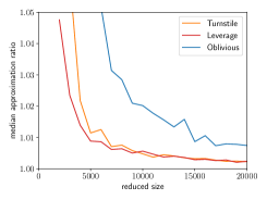
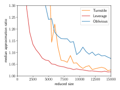
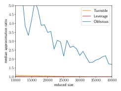
$\ell_{1}$ Regression

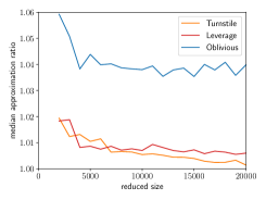
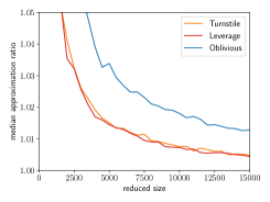
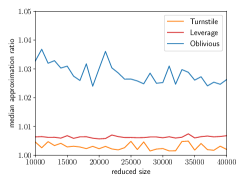
Figure 1: Comparison of the approximation ratios for logistic regression, and $\ell_{1}$ regression on various real-world datasets. The new turnstile data stream sampler (orange) is compared to plain leverage score sampling (red), and to plain oblivious sketching (blue). The plots indicate the median of approximation ratios taken over 21 repetitions for each reduced size. Best viewed in colors, lower is better.

We demonstrate the performance of our novel turnstile $\ell_{p}$ sampler. Recall, that our algorithm is a hybrid between an oblivious sketch and a leverage score sampling algorithm. It thus makes most sense to compare to pure oblivious sketching as well as to pure off-line leverage score sampling. To this end, we implement our new algorithm into the experimental framework of the near-linear oblivious sketch of Munteanu et al., (2023), and add the code of Munteanu et al., (2022) for $\ell_{1}$ leverage score sampling.

Our a priori hypothesis from the theoretical knowledge on the three regimes is that the performance should be somewhere in the middle between the performances of the competitors. Ideally, we would want our algorithm to perform as closely as possible to off-line leverage score sampling.

The following real-world datasets have become standard baselines to measure the performance of data reduction algorithms for logistic regression and $\ell_{1}$ regression: Covertype, Webspam, and KDDCup, see Section I.2 for details. For each dataset, and each of the two problems, we first solve the original large instance to optimality to obtain $z_{opt}$. We then run the data reduction algorithms, for varying target coreset resp. sketch sizes, and solve the reduced and reweighted problem to optimality to obtain the approximation $\tilde{z}$. For each target size, we repeat this process $21$ times and plot in Figure 1 the median of the resulting approximation ratios $f(\tilde{z})/f(z_{opt})$. We experienced convergence problems using the scipy optimizer for the non-differentiable $\ell_{1}$ loss. Thus, for $\ell_{1}$ regression, $z_{opt}$ denotes the best (though not necessarily optimal) solution found. The results are consistent across all settings: our new turnstile sampler outperforms pure oblivious sketching by a large margin. Its performance lies between the two competitors and is very close to off-line leverage score sampling. In some cases, it even performs slightly better for $\ell_{1}$ regression, which is likely due to the reported inaccuracies of the scipy optimizer, rather than the reduction algorithms.

The experiments affirm our hypothesis, and corroborate the usefulness of our novel turnstile $\ell_{p}$ leverage score sampling sketch in practical applications. We refer to Appendix I for more experiments using $p=1.5$, and a mixture of $\ell_{1}+\ell_{2}$ leverage scores, as well as details on data, computing environment, running times, and memory requirements.

5 Conclusion

We generalize the turnstile $\ell_{2}$ row sampling algorithm of Mahabadi et al., (2020) to work for all $p\in[1,2]$ using novel statistical tests that rely only on the CountSketch data structure, rather than requiring auxiliary or $p$-specific sketches. This is used to simulate $\ell_{p}$ leverage score sampling over a turnstile data stream. The combination of different $\ell_{p}$ distributions and uniform sampling extends our methods to logistic regression and $\ell_{p}$ generalizations of linear, ReLU, and probit regression losses. Our experiments show good performance for $\ell_{p}$ and logistic regression as compared to pure oblivious sketching and off-line sampling. The most intriguing open question is whether it is possible to simulate the construction of $\ell_{p}$ spanning sets Woodruff and Yasuda, 2023a ; Bhaskara et al., (2023) in turnstile data streams, which would bring larger powers of $d$ down to near-optimal linear dependence Munteanu and Omlor, (2024).

Appendix A Preliminaries

We are given a data matrix $A\in\mathbb{R}^{n\times d}$ with row vectors $a_{i},\dots a_{n}\in\mathbb{R}^{d}$ presented in a turnstile data stream. We assume that $n\gg d$. Further let $p\in[1,2]$ have a fixed value. Let $s_{i}\geq u_{i}^{(p)}+\frac{1}{n}$ where $u_{i}^{(p)}=\sup_{x\in\mathbb{R}^{d}\setminus\{0\}}\frac{|a_{i}x|^{p}}{\lVert Ax\rVert_{p}^{p}}$ are the $\ell_{p}$ leverage scores (see Definition H.1). Our goal is to develop an algorithm that samples row $i$ with probability $p_{i}\gtrsim\frac{ks_{i}}{S}$ in one pass over a turnstile data stream and determine weights $w_{i}\approx\frac{1}{p_{i}}$. We allow an error controlled by a parameter $\varepsilon>0$ in both, the sampled vector as well as the weight.

Appendix B The algorithms

Our first algorithm (Algorithm 1) determines heavy rows of a matrix $A$. It is a modification of the CountSketch (Charikar et al.,, 2004), that performs additional statistical tests on $s$ repetitions of the sketch to 1) determine a suitable threshold $M_{0}$ using the $0.65$-percentile among the $s$ repetitions, relative to which any row will be considered ’heavy’, 2) estimate the $\ell_{p}$ norm of the current row up to $(1\pm\varepsilon)$ error using the median among the $s$ repetitions, and compares the estimate to the threshold, and 3) find a representative element among the $s$ repetitions using the median again, to find an approximation of the row that lies close to most other approximations. This will ensure that it also lies close to the original input row, which it represents. See the main text for more details.

Our second algorithm (Algorithm 2) multiplies random scaling factors $t_{i}^{-1/p}$, where $t_{i}\sim{U}(0,1)$ to the rows of a matrix $A$ to get a new Matrix $A^{\prime}=TA$, where $T=\operatorname{diag}(t_{1}^{-1/p},\ldots,t_{n}^{-1/p})$ is a diagonal $n\times n$ matrix. Then Algorithm 1 is applied to determine the heavy rows of $A^{\prime}P$. Hereby $A$ is presented in a turnstile data stream, and $P$ is a conditioning matrix that is obtained in a postprocessing step after the stream has reached its end. This can be done using another turnstile sketching primitive applied to the stream that represents $A$ in parallel to our algorithm. The postprocessing step is then completed by right-multiplication of our sketch with $P$ (in most of our analysis $P=I$; other choices are discussed later in the applications of Section 3). If $r$ and $s$ are sufficiently large, then we can guarantee that $A^{\prime}$ has at least a certain number of heavy rows, the (roughly) $k$ largest of which are back transformed to their original sign, scale and basis, and returned as an approximate sample $S$ together with estimated sampling probabilities. This is done by calculating a threshold $\alpha$ which is the smallest approximated $\ell_{p}$ norm of the $k$ largest elements. For $(i,\tilde{a}_{i}P^{-1},w_{i})\in S$ the first entry is the index of a row $a_{i}$ of $A$, the second entry is a slightly perturbed row $\tilde{a}_{i}P^{-1}\approx a_{i}$, and the third entry is a weight which is roughly the inverse of the sampling probabilities $p_{i}\approx\min\{1,{\lVert\tilde{a}_{i}\rVert_{p}^{p}}/{\alpha}\}\approx\min\{1,{\lVert a_{i}P\rVert_{p}^{p}}/{\lVert AP\rVert_{p}^{p}}\}$.

Appendix C Outline of the analysis

• We first prove some technical lemmas that are used multiple times and give intuitions about how parts of the analysis work. In particular, we analyze sums of Bernoulli random variables, medians and other percentiles, as well as the expected $\ell_{p}$ norm of a random bucket.

• We analyze Algorithm 1. Here, we show that there is an upper bound for $M_{0}$ which guarantees that it finds and returns all ’heavy’ rows. Further, we show that there is a lower bound for the threshold $M_{0}$, which guarantees that any element returned by the algorithm is approximated up to a relative error of $\varepsilon$.

• We then proceed by analyzing a slightly modified version of Algorithm 2 (see Appendix F for details). We first give a high level intuition of how the algorithm works. We prove that the probability of sampling row $i$ is greater or equal to $(1-\varepsilon){\lVert a_{i}P\rVert_{p}^{p}}/{\alpha}\approx c\cdot{k\lVert a_{i}P\rVert_{p}^{p}}/{\lVert AP\rVert_{p}^{p}}$ for an appropriate $\alpha$ (and constant $c$) and that the number of samples is in the interval $[k,2k]$. We then use the properties proven in 2) to show that the norm of each row is approximated up to a relative error of $\varepsilon$. Finally, we analyze the weights for which we show that they are roughly the inverse sampling probabilities and that they can be used to approximate $\lVert AP\rVert_{p}^{p}$ up to a factor $(1\pm\varepsilon)$.

• We show that if we can sample from two distributions $p_{i},p_{i}^{\prime}$, we can also sample from a joint distribution where the sampling probability is roughly $\frac{p_{i}+p_{i}^{\prime}}{2}$. In particular, we use this to combine Algorithm 2 with uniform sampling to sample with probability proportional to $\frac{\lVert a_{i}P\rVert_{p}^{p}}{\lVert AP\rVert_{p}^{p}}+\frac{1}{n}$.

• We show how our results can be applied to construct an $\varepsilon$-coresets for the $\ell_{p}$ variants of linear regression, ReLU regression, probit regression, as well as logistic regression.

Appendix D Tools for the analysis

Let us start with some facts following from well known results of probability theory. The first fact is about the median of Bernoulli random variables. The lemma will be crucial for arguments regarding the median or other percentiles and to obtain bounds on the number of samples.

Lemma D.1.

Let $m\in\mathbb{N}$ and $0<\delta<1$. Let $X_{1},\dots,X_{m}$ be a sequence of independent Bernoulli random variables with $P(X_{i}=1)=p>0.075$. If $m\geq 3\ln(2/\delta)/0.025^{3}$ then with probability at least $1-\delta$ it holds that $X=\sum_{i=1}^{m}X_{i}=|\{i\mid X_{i}=1\}|\in(1\pm 0.025)pm$.

Proof.

Let $X=\sum_{i=1}^{m}X_{i}$ be the number of $1$’s in $\{X_{1}\dots X_{m}\}$. Since $X$ is a sum of Bernoulli random variables, the expected value of $X$ equals $\mathbb{E}(\sum_{i=1}^{m}X_{i})=pm$. By Chernoff’s bound it holds that

$$P(|X-pm|>0.025pm)\leq 2\exp\left(-\frac{0.025^{2}pm}{3}\right)\leq 2\exp\left(-\frac{0.025^{3}m}{3}\right)\leq\delta.$$

∎

The next lemma is similar to the previous one but handles Bernoulli random variables with small expected sum.

Lemma D.2.

Let $m\in\mathbb{N}$ and $0<\delta<1$. Let $X_{1},\dots,X_{m}$ be a sequence of independent Bernoulli random variables with $P(X_{i}=1)=p_{i}$ and let $k\geq 20\ln(2/\delta)$. If $\operatorname*{\mathbb{E}}(X)\leq 9k$ then with probability at least $1-\delta$ it holds that

$$X=\sum\nolimits_{i=1}^{m}X_{i}=|\{i\mid X_{i}=1\}|\in[\operatorname*{\mathbb{E}}(X)-k,\operatorname*{\mathbb{E}}(X)+k].$$

Proof.

We will prove this by using Bernstein’s inequality. First, note that $\operatorname*{\mathbb{E}}(\sum_{i=1}^{m}X_{i}^{2})=\operatorname*{\mathbb{E}}(\sum_{i=1}^{m}X_{i})=\operatorname*{\mathbb{E}}(X)\leq 9k$ since $X_{i}$ are Bernoulli random variables. Second, note that $X_{i}\leq 1$. Thus using Bernstein’s inequality we get that

$$P(|X-\operatorname*{\mathbb{E}}(X)|\geq k)\leq 2\exp\left(-\frac{k^{2}/2}{\operatorname*{\mathbb{E}}(X)+k/3}\right)\leq 2\exp\left(-\frac{k}{20}\right)\leq\delta.$$

∎

An important property of a sum with random signs is that it preserves the $\ell_{2}$ norm of the entries. The following lemma uses this fact and shows the relation of the expected value of the $p$th power of a sum with random signs over the elements of a vector $v$ to its $\ell_{p}$ norm $\lVert v\rVert_{p}^{p}$.

Lemma D.3.

Let $v_{1},\dots v_{n}\in\mathbb{R}^{d}$ and let $\sigma_{1},\ldots,\sigma_{n}\in\{-1,1\}$ be uniform and pairwise independent random signs. If $p\leq 2$ then it holds that $\mathbb{E}(\lVert\sum_{i=1}^{n}\sigma_{i}v_{i}\rVert_{p}^{p})\leq\sum_{i=1}^{n}\lVert v_{i}\rVert_{p}^{p}$.

Proof.

First note that for uniform and pairwise independent random signs we have that

$$\operatorname*{\mathbb{E}}\left(\left\|\sum_{i=1}^{n}\sigma_{i}v_{i}\right\|_{p}^{p}\right)=\operatorname*{\mathbb{E}}\left(\sum_{j=1}^{d}\left|\sum_{i=1}^{n}\sigma_{i}v_{ij}\right|^{p}\right)=\sum_{j=1}^{d}\operatorname*{\mathbb{E}}\left(\left|\sum_{i=1}^{n}\sigma_{i}v_{ij}\right|^{p}\right).$$

Khintchine’s inequality (see Haagerup,, 1981) followed by the standard inter-norm inequality yield

$$\mathbb{E}\left(\left|\sum_{i=1}^{n}\sigma_{i}v_{ij}\right|^{p}\right)\leq\lVert v^{(j)}\rVert_{2}^{p}\leq\lVert v^{(j)}\rVert_{p}^{p}$$

where $v^{(j)}\in\mathbb{R}$ is the vector with coordinates $v_{ij}$ for $i\in[n]$. Combining the previous two inequalities we get that

$$\operatorname*{\mathbb{E}}\left(\left\|\sum_{i=1}^{n}\sigma_{i}v_{i}\right\|_{p}^{p}\right)\leq\sum_{j=1}^{d}\lVert v^{(j)}\rVert_{p}^{p}=\sum_{i,j\in[n]\times[d]}|v_{ij}|^{p}=\sum_{i=1}^{n}\lVert v_{i}\rVert_{p}^{p}$$

∎

Some notation

Consider a bucket $B$ consisting of a set of indices together with the corresponding set of random signs we define $G_{p}(B)=\lVert\sum_{i\in B}\sigma_{i}a_{i}\rVert_{p}$. The specific signs $\sigma_{i}=\sigma_{i,j},j\in[s]$ will be clear from the context.

Appendix E Analysis of Algorithm 1

High level idea

For $k\in[n]$ let $S_{L}(k,A)\subset[n]$ be the subset of the $k$ indices of elements with the largest $\ell_{p}$ norm (ties are broken arbitrarily) and let $S_{R}(k,A)=[n]\setminus S_{L}(k,A)$ be the subset of the remaining indices. If $A$ is clear from the context we simply write $S_{L}(k)$ and $S_{R}(k)$. If $k$ is also clear from the context we just write $S_{L}$ and $S_{R}$.

The idea of Algorithm 1 is that if we hash the elements to $r$ buckets, then for $k=r/20$, at least $r-r/20$ buckets, do not contain any large element of $S_{L}(k)$. Further the expected squared $\ell_{2}$ norm of a bucket is $M/r$ for $M=\sum_{i\in S_{R}(k)}\lVert a_{i}\rVert_{p}^{p}$. Using Lemma D.3 and the union bound we can extend this result showing that with probability at least $1-1/4-1/20$, the contribution of a bucket $B$ is $G(B)^{p}\leq 4M/r$.

The argument can also be applied to the buckets containing a certain index $i$, i.e., if we consider a bucket $B_{i}$ containing the element $i$ then with probability at least $1-1/4-1/20$ we have that $\lVert B_{i}-\sigma_{i}a_{i}\rVert_{p}^{p}=\lVert\sum_{j\in B\setminus\{i\}}\sigma_{j}a_{j}\rVert_{p}^{p}\leq 4M/r$. Thus if $\lVert a_{i}\rVert_{p}^{p}\gtrsim\frac{M}{\varepsilon^{p}r}$ then most of the buckets containing element $i$ will be close to $a_{i}$ and using the median, which is the approximation $\tilde{a}_{i}$ calculated by Algorithm 1, we can approximate the large elements exceeding a fraction of $\gamma M$ up to an error of $\varepsilon$ with respect to their $\ell_{p}$ norm by setting $r=O(\frac{1}{\gamma\varepsilon^{p}})$.

In addition to the definitions given in the high level idea, we define

$$M^{\prime}=\inf\{w\in\mathbb{R}_{\geq 0}\mid P(G(B)^{p}\leq w)\geq 0.6\}$$

to be the (theoretical) $.6$-percentile of the $\ell_{p}^{p}$ norm contributions of buckets. The following Lemma yields an upper and a lower bound for $M_{0}$:

Lemma E.1.

If $s\geq 3\ln(2/\delta)/0.025^{3}$, then the value of $M_{0}$ in Algorithm 1 satisfies

$$M^{\prime}\leq M_{0}\leq 4M/r$$

with failure probability at most $2\delta$.

Proof.

Let $S_{L}=S_{L}(r/20)$ be the set of the $r/20$ indices with the largest $\ell_{p}$ norm and $S_{R}=[n]\setminus S_{L}$. Let $M=\sum_{i\in S_{R}}\lVert a_{i}\rVert_{p}^{p}$. Consider any bucket $B$. The probability that $B$ contains any specific element is $1/r$. By a union bound, the probability that $B$ contains an element of $S_{L}$ is bounded by $P(B\cap S_{L}\neq\emptyset)\leq r/20\cdot 1/r=1/20$. Further denoting by $P(S)$ for a set $S$ the probability that $S=B\setminus S_{L}$ and using Lemma D.3 it holds that

$$\operatorname*{\mathbb{E}}(G_{p}(B\setminus S_{L})^{p}) =\sum_{S\subset S_{R}}P(S)\operatorname*{\mathbb{E}}\left(\left\|\sum_{i\in S}\sigma_{i}a_{i}\right\|_{p}^{p}\right)\leq\sum_{S\subset S_{R}}P(S)\left(\sum_{i\in S}\lVert a_{i}\rVert_{p}^{p}\right).$$

Now, by double counting the last term, we also have that

$$\sum_{S\subset S_{R}}P(S)\left(\sum_{i\in S}\lVert a_{i}\rVert_{p}^{p}\right)=\sum_{i\in S_{R}}\lVert a_{i}\rVert_{p}^{p}\left(\sum_{S\subset S_{R},i\in S}P(S)\right)=\sum_{i\in S_{R}}\lVert a_{i}\rVert_{p}^{p}\cdot P(i\in B)=\sum_{i\in S_{R}}\frac{1}{r}\cdot\lVert a_{i}\rVert_{p}^{p}=M/r.$$

Thus using Markov’s inequality we have that $G_{p}(B\setminus S_{L})^{p}\leq 4M/r$ with probability at least $1-1/4$. Using the union bound we have that with probability at least $1-1/4-1/20=0.7$, an arbitrary bucket $B$ contains no element of $S_{L}$ and $G_{p}(B\setminus S_{L})^{p}\leq 4M/r$.

Since $s\geq 3\ln(2/\delta)/0.025^{3}$, Lemma D.1 implies that at least $0.675\cdot s$ many random buckets satisfy these properties with failure probability at most $\delta$, so in particular this holds for the (realized) $.65$-percentile $M_{0}$. We conclude that $M_{0}\leq 4M/r$.

The lower bound also follows by Lemma D.1 for $s\geq 3\ln(2/\delta)/0.025^{3}$, which implies that the (theoretical) $.6$-percentile is not exceeded by more than $.025$. Specifically, this yields $|\{j\in[s]\mid G(B_{j,1})^{p}\leq M^{\prime}\}|\leq 0.625s$. Consequently the (realized) $0.65$-percentile $M_{0}$ is larger than $M^{\prime}$. The failure probability is again bounded by at most $\delta$, and the overall failure probability is bounded by $2\delta$ by another union bound, which concludes the proof. ∎

In the following lemma, these bounds will be used to show that with high probability all elements in the output $L$ of Algorithm 1 are close to the original rows. Further it shows that all rows with large $\ell_{p}$ norm will be in $L$.

Lemma E.2.

If $s\geq 3\ln(2n/\delta)/0.025^{3}$, $r\geq 50$, $0<\varepsilon\leq 1/3$ and $M^{\prime}\leq M_{0}$, then the following holds with failure probability at most $\delta$: For any $i\in[n]$ with $v_{i}\geq(12/\varepsilon)^{p}M^{\prime}$ it holds that $\lVert a_{i}\rVert_{p}^{p}\geq(3/\varepsilon)^{p}M^{\prime}$. Further, for any $i\in[n]$ with $\lVert a_{i}\rVert_{p}^{p}\geq(3/\varepsilon)^{p}M^{\prime}$ it holds that $v_{i}=(1\pm\varepsilon)\lVert a_{i}\rVert_{p}^{p}$. In particular, this implies that for any $i$ with $\lVert a_{i}\rVert_{p}^{p}\geq(12/\varepsilon)^{p}M^{\prime}/(1-\varepsilon)$ it holds $i\in L$. Finally, it holds for $S_{i}:=\{j\in[s]\mid\lVert\tilde{a}_{i,j}-a_{i}\rVert_{p}\leq\varepsilon\|a_{i}\|_{p}/9\}$ that $|S_{i}|\geq s/2$.

Proof.

By Lemma E.1, it holds that $M^{\prime}\leq M_{0}$ with probability $1-\delta$.

We show the first claim by contraposition: rows $a_{i}$ with small norms, i.e., $\lVert a_{i}\rVert_{p}^{p}<(3/\varepsilon)^{p}M^{\prime}$ will not be part of the output $L$. Fix $i\in[n]$ and for each repetition $j\in[s]$ let $B(i,j)$ be the bucket that contains $i$. We set $b_{i,j}=\sum_{l\in B(i,j)\setminus\{i\}}\sigma_{l,j}a_{l}$ to be the content of the bucket after sketching all data, but with the contribution of $a_{i}$ removed. We set

$$M^{\prime\prime}=\inf\{w\in\mathbb{R}_{\geq 0}\mid P(G(B\setminus\{i\})^{p}\leq w)\geq 0.575\}.$$

Note that for any bucket $B$ it holds that $P(i\in B)=1/r\leq 0.02$. Thus, we have that

$$P(G(B\setminus\{i\})^{p}\leq M^{\prime})\geq P(G(B)^{p}\leq M^{\prime})-P(i\notin B)\geq 0.58>0.575.$$

and consequently $M^{\prime\prime}\leq M^{\prime}$.

By definition of the $.575$-percentile $M^{\prime\prime}$ and applying Lemma D.1, we get that

$$\lVert b_{i,j}\rVert_{p}^{p}\leq M^{\prime\prime}\leq M^{\prime}$$

holds for at least half of the indices of $j\in[s]$ up to failure probability at most $\delta/n$ which will be assumed in the remainder of the proof.

For all $i$ and $j$ that satisfy $\lVert b_{i,j}\rVert_{p}^{p}\leq M^{\prime}$, we have that

$$G(B(i,j))^{p} =\lVert\sigma_{i,j}a_{i}+b_{i,j}\rVert_{p}^{p}\leq(\lVert a_{i}\rVert_{p}+M^{\prime 1/p})^{p}$$

$$\leq(2\max\{\lVert a_{i}\rVert_{p},M^{\prime 1/p}\})^{p}\leq\max\{4\lVert a_{i}\rVert_{p}^{p},4M^{\prime}\}.$$

Then it also holds that $v_{i}=\operatorname*{\mathbf{median}}_{j\in[s]}\lVert\tilde{a}_{i,j}\rVert_{p}^{p}\leq\max\{4\lVert a_{i}\rVert_{p}^{p},4M^{\prime}\}$. Thus, we can conclude that if index $i$ satisfies $\lVert a_{i}\rVert_{p}^{p}<(3/\varepsilon)^{p}M^{\prime}\leq(3/\varepsilon)^{p}M_{0}$ then it holds that

$$v_{i}<\max\{(12/\varepsilon)^{p}M_{0},4M^{\prime}\}\leq(12/\varepsilon)^{p}M_{0}$$

and consequently $i\notin L$.

Next, we show that rows with larger norm $\lVert a_{i}\rVert_{p}^{p}\geq(3/\varepsilon)^{p}M^{\prime}$ are well approximated assuming that $\lVert b_{i,j}\rVert_{p}^{p}\leq M^{\prime}$. Let $\gamma:=\frac{M^{\prime}}{\lVert a_{i}\rVert_{p}^{p}}\leq(\varepsilon/3)^{p}$. Then by the triangle inequality it holds that

$$G(B(i,j))^{p}=\lVert\sigma_{i,j}a_{i}+b_{i,j}\rVert_{p}^{p}\leq(1+\gamma^{1/p})^{p}\lVert a_{i}\rVert_{p}^{p}\leq(1+3\gamma^{1/p})\lVert a_{i}\rVert_{p}^{p}\leq(1+\varepsilon)\lVert a_{i}\rVert_{p}^{p}$$

and similarly we have

$$G(B(i,j))^{p}=\|\sigma_{i,j}a_{i}+b_{i,j}\|_{p}^{p}\geq(1-3\gamma^{1/p})\lVert a_{i}\rVert_{p}^{p}\geq(1-\varepsilon)\lVert a_{i}\rVert_{p}^{p}.$$

Since $\|b_{i,j}\|_{p}^{p}\leq M^{\prime}$ holds for at least half of the indices $j\in[s]$ we can conclude that

$$v_{i}=\operatorname*{\mathbf{median}}_{j\in[s]}\lVert\tilde{a}_{i,j}\rVert_{p}^{p}\in\left[(1-\varepsilon)\lVert a_{i}\rVert_{p}^{p},(1+\varepsilon)\lVert a_{i}\rVert_{p}^{p}\right].$$

Finally, we show that for $i$ with $i\in L$ it holds that $\lVert\tilde{a}_{i,j}-a_{i}\rVert_{p}\leq(\varepsilon/9)\lVert a_{i}\rVert_{p}$ and that $|S_{i}|\geq s/2$. Using that $\varepsilon\leq 1/3$ we have for $i\in[n]$ with $v_{i}\geq(12/\varepsilon)^{p}M_{0}$ that

$$\lVert\tilde{a}_{i,j}-a_{i}\rVert_{p}^{p}=\lVert b_{i,j}\rVert_{p}^{p}\leq M^{\prime}\leq M_{0}\leq(\varepsilon/12)^{p}\,v_{i}\leq(\varepsilon/12)^{p}(1+\varepsilon)\lVert a_{i}\rVert_{p}^{p}\leq(\varepsilon/9)^{p}\lVert a_{i}\rVert_{p}^{p}$$

which also yields

$$|\{j\in[s]\mid\lVert\tilde{a}_{i,j}-a_{i}\rVert_{p}\leq\varepsilon\|a_{i}\|_{p}/9\}|\geq s/2.$$

By the union bound, these properties hold for all $i$ simultaneously with probability at least $1-O(\delta)$. Rescaling $\delta$ by a constant concludes the proof. ∎

We are now ready to prove that Algorithm 1 works as intended for the right choice of $r$ and $s$:

Theorem E.3 (copy of Theorem 2.1).

Let $\varepsilon,\delta\in(0,1/20],\gamma\in(0,1)$. Let $L$ be the list of tuples in the output of Algorithm 1. Further let $S_{R}(r/20)$ be the subset of rows excluding the $r/20$ largest $\ell_{p}$ norms and let $M=\sum_{i\in S_{R}}\lVert a_{i}\rVert_{p}^{p}$. If $r=8\gamma^{-1}\cdot(12/\varepsilon)^{p}$ and $s\geq 3\ln(6n/\delta)/0.025^{3}$ then with probability at least $1-\delta$, the following properties hold: for any element $(i,\tilde{a}_{i})\in L$ it holds that $\lVert\tilde{a}_{i}-a_{i}\rVert_{p}\leq(\varepsilon/3)\lVert a_{i}\rVert_{p}$ and $\lVert\tilde{a}_{i}\rVert_{p}^{p}=(1\pm\varepsilon)\lVert a_{i}\rVert_{p}^{p}$. Further, for any $i\in[n]$ with $\lVert a_{i}\rVert_{p}^{p}\geq\gamma M$ it holds that $i\in L$.

Proof of Theorem 2.1/E.3.

The statements of Lemma E.1 and Lemma E.2 hold with failure probability at most $\delta=2(\delta/3)+(\delta/3)$ using the union bound. Then we have that $M^{\prime}\leq M_{0}\leq 4M/r$ and for any $i\in L$ it holds that $v_{i}\geq(12/\varepsilon)^{p}M_{0}\geq(12/\varepsilon)^{p}M^{\prime}$. Lemma E.2 yields that $v_{i}=(1\pm\varepsilon)\lVert a_{i}\rVert_{p}^{p}$. For the set $S_{i}=\{j\in[s]\mid\lVert a_{i}-\tilde{a}_{i,j}\rVert_{p}\leq\varepsilon\lVert a_{i}\rVert_{p}/9\}$ we have that $|S_{i}|\geq s/2$.

For any elements $j,j^{\prime}\in S_{i}$ we have

$$\lVert\tilde{a}_{i,j}-\tilde{a}_{i,j^{\prime}}\rVert_{p}\leq\lVert\tilde{a}_{i,j}-a_{i}\rVert_{p}+\lVert a_{i}-\tilde{a}_{i,j^{\prime}}\rVert_{p}\leq 2\varepsilon\lVert a_{i}\rVert_{p}/9$$

by the triangle inequality. It follows that $\operatorname*{\mathbf{median}}_{j^{\prime}\in[s]}\{\lVert\tilde{a}_{i,j}-\tilde{a}_{i,j^{\prime}}\rVert_{p}\}\leq 2\varepsilon\lVert a_{i}\rVert_{p}^{p}/9$ since $|S_{i}|\geq s/2$.

Let $\tilde{a}_{i}=\tilde{a}_{i,j}$ for $j\in[s]$ minimizing $\operatorname*{\mathbf{median}}_{j^{\prime}\in[s]}\{\lVert\tilde{a}_{i,j}-\tilde{a}_{i,j^{\prime}}\rVert_{p}^{p}\}$. Again since $|S_{i}|\geq s/2$ there must be at least one element in $j^{\prime}\in S_{i}$ with $\lVert\tilde{a}_{i,j}-\tilde{a}_{i,j^{\prime}}\rVert_{p}\leq 2\varepsilon\lVert a_{i}\rVert_{p}/9$. Using the triangle inequality again we get that

$$\lVert\tilde{a}_{i}-a_{i}\rVert_{p}=\lVert\tilde{a}_{i,j}-a_{i}\rVert_{p}\leq\lVert\tilde{a}_{i,j}-\tilde{a}_{i,j^{\prime}}\rVert_{p}+\lVert\tilde{a}_{i,j^{\prime}}-a_{i}\rVert_{p}\leq(2\varepsilon/9+\varepsilon/9)\lVert a_{i}\rVert_{p}\leq\varepsilon\lVert a_{i}\rVert_{p}/3.$$

We note that since $\lVert\tilde{a}_{ij}-a_{i}\rVert_{p}\leq{\varepsilon}\lVert a_{i}\rVert_{p}/3$ holds, we have by the triangle inequality that

$$\lVert\tilde{a}_{ij}\rVert_{p}^{p}\leq(\lVert a_{i}\rVert_{p}+\lVert\tilde{a}_{ij}-a_{i}\rVert_{p})^{p}\leq(1+\varepsilon)\lVert a_{i}\rVert_{p}^{p}$$

and

$$\lVert\tilde{a}_{ij}\rVert_{p}^{p}\geq(\lVert{a_{i}}\rVert_{p}-\lVert\tilde{a}_{ij}-a_{i}\rVert_{p})^{p}\geq(1-\varepsilon)\lVert a_{i}\rVert_{p}^{p}.$$

Finally, since $M^{\prime}\leq M_{0}\leq 4M/r$, or equivalently $M^{\prime}r/4\leq M_{0}r/4\leq M$, we also have for any $i$ with $\lVert a_{i}\rVert_{p}^{p}\geq\gamma M$ that

$$\lVert a_{i}\rVert_{p}^{p}\geq{\gamma M}\geq\gamma rM_{0}/4$$

and thus by Lemma E.2

$$v_{i}\geq(1-\varepsilon)\lVert a_{i}\rVert_{p}^{p}\geq\frac{1}{2}\cdot\frac{\gamma rM_{0}}{4}\geq(12/\varepsilon)^{p}M_{0}.$$

which implies that $i\in L$. ∎

Appendix F Analysis of Algorithm 2

High level idea

Consider the matrix $A\in\mathbb{R}^{n\times 1}$ consisting of $n$ copies of the row $1$. If we multiply each row with $t_{i}^{-1}$ where $t_{i}\in(0,1]$ are drawn uniformly at random then what roughly happens is that the new matrix $A^{\prime}$ with rows $a^{\prime}_{i}=a_{i}/t_{i}$ consists of the rows $n,n/2,n/3,\dots,n/(n-1),1$. We then have that $\lVert A^{\prime}\rVert_{1}=\Theta(n\log(n))$ and the $k$ largest elements of $A^{\prime}$ are bounded from below by $n/k$. Or in other words $M=(n\log(n))$ and we want to find all rows with $\ell_{1}$ norm greater or equal to $n/k$. If we now apply Algorithm 1 to $A^{\prime}$ with $r=O(k\log(n)/\varepsilon)$ then all elements with $a_{i}^{\prime}\geq{n/k}=\Theta(M/(k\log(n)))$ will be in $L$ with high probability. The challenge will be to control the randomness of the variables $t_{i}$ and to generalize the idea to arbitrary instances and different $p$’s.

Instead of analyzing Algorithm 2 as presented, we analyze a slightly modified version, where Algorithm 1 is applied twice in parallel. The main purpose of the modification is to keep the analysis clean and simple. The presented Algorithm 2 is likely to have the same properties up to small constant factors but the analysis would require to work with conditional probabilities which only leads to additional technicalities that distract from understanding the main ideas of our algorithm.

Modification of Algorithm 1

To simplify the analysis, we run Algorithm 1 twice with two independent copies of the scaling random variables $t_{i},i\in[n]$. The first copy is used to compute $\alpha$ and the second generates the sample using the value of $\alpha$ from the first copy. This makes the estimate $\alpha$ independent of the sample and avoids purely technical difficulties in the analysis. However, it is likely not necessary and is therefore not presented in the pseudo code. In the first iteration, we use an increased value of $k^{\prime}=(3/2)k$ and we stop after defining $\alpha$ (line 9). In the second iteration, we skip lines 8-9 and use $\alpha$ from the previous iteration.

We define $S\subseteq L$ to be the set of indices with $\lVert\tilde{a}_{i}\rVert_{p}^{p}\geq\alpha$ returned at the end. We assume that $t_{i}\in(0,1]$ are drawn i.i.d. uniformly at random and $A^{\prime}=TA\in\mathbb{R}^{n\times d}$ is the matrix with rows $a_{i}^{\prime}=t_{i}^{-1/p}a_{i}$.

Our main theorem is that given $k\in[n]$ with an appropriate choice of $r,s$ Algorithm 2 returns a subsample $S\subseteq[n]\times\mathbb{R}^{d}\times\mathbb{R}_{\geq 1}$ such that $|S|\in[k,2k]$, index $i$ is sampled with probability at least $\min\{1,\frac{k\lVert a\rVert_{p}^{p}}{\lVert A\rVert_{p}^{p}}\}$ and for $(i,\tilde{a}_{i},w_{i})\in S$ we have that $\lVert\tilde{a}_{i}-a_{i}\rVert_{p}=(\varepsilon/3)\lVert a_{i}\rVert_{p}$ and $w_{i}=(1\pm\varepsilon)P(i\in S)^{-1}$. Further we can use the weights to approximate $\lVert A\rVert_{p}^{p}$ up to a factor of $(1\pm\varepsilon)$.

Theorem F.1 (copy of Theorem 2.2).

If we apply the modified version of Algorithm 2 (see Appendix F) with $0<\varepsilon,\delta\leq 1/20$, $k\geq 160\ln(12/\delta)$, $r\geq 32k\ln(n)\cdot(72/\varepsilon)^{p}$, and $s\geq 3\ln(36n/\delta)/0.025^{3}$, then with probability at least $1-\delta$ it holds that

• $|S|\in[k,2k]$,

• index $i\in S$ is sampled with probability
            $p_{i}:=P(i\in S)\geq\min\left\{1,\frac{k\lVert a\rVert_{p}^{p}}{\lVert A\rVert_{p}^{p}}\right\},$

• if $i\in S$ then $\lVert\tilde{a}_{i}-a_{i}\rVert_{p}\leq(\varepsilon/3)\lVert a_{i}\rVert_{p}$,

• if $i\in S$ then $w_{i}=(1\pm\varepsilon)\frac{1}{p_{i}}$,

• $\sum_{i\in S}w_{i}\lVert\tilde{a}_{i}\rVert_{p}^{p}=(1\pm\varepsilon)\lVert A\rVert_{p}^{p}$.

To support readability, the proof of Theorem 2.2/F.1 is divided into multiple Lemmas.

Our first Lemma considers the unique number $N(k)\in\mathbb{R}_{\geq 0}$ such that the expected number of elements $i\in[n]$ with $\lVert a_{i}^{\prime}\rVert_{p}^{p}\geq N(k)$ is $k$. The properties that we show in this Lemma will allow to show that the number of elements is $|S|\in[k,2k]$. Further it will be used later to show that the largest $2k$ rows of $A^{\prime}$ have a norm large enough to be in $L$ with failure probability at most $\delta$. Before we state the lemma, we need to give some more definitions:

Recall that $S_{L}(k,A)\subseteq[n]$ is the set of indices of the elements with the $k$ largest norms (of $A$) and $S_{R}(k,A)=[n]\setminus S_{L}$. We set $M(A,k):=\sum_{i\in S_{R}(k,A)}\lVert a_{i}\rVert_{p}^{p}$.

We will show that all indices where $\lVert a_{i}\rVert_{p}^{p}\geq\lVert A\rVert_{p}^{p}/k$ will be sampled with probability at least $1-\delta$. The exact value of $\lVert a_{i}\rVert_{p}^{p}$ does not matter but if it gets large, it makes the analysis more complicated. Since we want to provide a good understanding of our analysis, instead of assuming that $\lVert a_{i}\rVert_{p}^{p}\geq\lVert A\rVert_{p}^{p}/k$ we define $A(k)\in\mathbb{R}^{n\times d}$ to be the truncated matrix that we get by scaling down the largest rows of $A$ so that all rows $a_{i}(k)$ of $A(k)$ satisfy $\lVert a_{i}(k)\rVert_{p}^{p}\geq\lVert A(k)\rVert_{p}^{p}/k$.

Definition F.2.

Let $u_{k}\in\mathbb{R}$ be the solution of the equation

$$\frac{u_{k}}{\sum_{i=1}^{n}\min\{u_{k},\lVert a_{i}\rVert_{p}^{p}\}}=\frac{1}{k}.$$

Then we define $A(k)$ to be the matrix with

$$a_{i}(k)=\begin{cases}\frac{u_{k}^{1/p}}{\lVert a_{i}\rVert_{p}}\cdot a_{i}&\lVert a_{i}\rVert_{p}^{p}>u_{k}\\ a_{i}&\lVert a_{i}\rVert_{p}^{p}\leq u_{k}.\end{cases}$$

In particular note that all elements $\lVert a_{i}\rVert_{p}^{p}>u_{k}$ are truncated to $\lVert a_{i}(k)\rVert_{p}^{p}=u_{k}$.

We already note the following properties of $A(k)$: it holds that $S_{R}(A(k),k)=S_{R}(A,k)$ and $\lVert A(k)\rVert_{p}^{p}\leq 2\cdot\sum_{i\in S_{R}(A,k/2)}\lVert a_{i}\rVert_{p}^{p}$. The first one follows immediately since there can be at most $k$ large rows that contribute $\lVert a_{i}\rVert_{p}^{p}\geq\lVert A\rVert_{p}^{p}/k$ and all others remain unchanged. The second claim will be proven in the following lemma.

Lemma F.3.

For $k\in[n]$ we set $N(k)\in\mathbb{R}_{\geq 0}$ to be the unique number such that the expected number of elements $i\in[n]$ with $\lVert a_{i}^{\prime}\rVert_{p}^{p}\geq N(k)$ is $k$. Then it holds that

$$\min\left\{\frac{\lVert A\rVert_{p}^{p}}{k},2M(A,k/2)\right\}\geq\frac{\lVert A(k)\rVert_{p}^{p}}{k}=N(k)\geq M(A,k)/k.$$

Proof.

We first prove that $N(k)=\frac{\lVert A(k)\rVert_{p}^{p}}{k}$. For $i\in[n]$ define the Bernoulli random variable $X_{i}=1$ if $t_{i}\leq k\lVert a_{i}(k)\rVert_{p}^{p}/\lVert A(k)\rVert_{p}^{p}$ and $X_{i}=0$ otherwise. Note that $X_{i}=1$ iff $\lVert a_{i}^{\prime}(k)\rVert_{p}^{p}=\lVert a_{i}(k)\rVert_{p}^{p}/t_{i}\geq\frac{\lVert A(k)\rVert_{p}^{p}}{k}$. Thus, $X_{i}=1$ holds with probability $p_{i}=\min\{1,k\lVert a_{i}(k)\rVert_{p}^{p}/\lVert A(k)\rVert_{p}^{p}\}=k\lVert a_{i}(k)\rVert_{p}^{p}/\lVert A(k)\rVert_{p}^{p}$ by definition of $A(k)$. Let $X=\sum_{i=1}^{n}X_{i}$. Observe that

$$\operatorname*{\mathbb{E}}(X)=\sum_{i=1}^{n}p_{i}=\sum_{i=1}^{n}k\lVert a_{i}(k)\rVert_{p}^{p}/\lVert A(k)\rVert_{p}^{p}=k.$$

To see this, note that the truncated largest rows satisfy $\lVert a_{i}(k)\rVert_{p}^{p}/\lVert A(k)\rVert_{p}^{p}=1/k$ by Definition F.2. Therefore their probability equals $p_{i}=1$. Now, if we increase their norms back to their original size, then the probabilities remain truncated at $1$, and thus do not change. Therefore $\operatorname*{\mathbb{E}}(X)=k$ holds also for the original matrix $A$. By definition of $N(k)$ we get that $N(k)=\frac{\lVert A(k)\rVert_{p}^{p}}{k}.$

Since $S_{R}(A(k),k)=S_{R}(A,k)$ it holds that

$$\frac{\lVert A\rVert_{p}^{p}}{k}\geq\frac{\lVert A(k)\rVert_{p}^{p}}{k}\geq\frac{M(A(k),k)}{k}=\frac{M(A,k)}{k}.$$

Further since $\frac{\lVert a_{i}(k)\rVert_{p}^{p}}{\lVert A(k)\rVert_{p}^{p}}\leq\frac{1}{k}$ we have that

$$\sum_{i\in S_{L}(A(k),k/2)}\lVert a_{i}(k)\rVert_{p}^{p}=\sum_{i\in S_{L}(A(k),k/2)}\lVert A(k)\rVert_{p}^{p}\cdot\frac{\lVert a_{i}(k)\rVert_{p}^{p}}{\lVert A(k)\rVert_{p}^{p}}\leq\sum_{i\in S_{L}(A(k),k/2)}\lVert A(k)\rVert_{p}^{p}\cdot\frac{1}{k}=\frac{\lVert A(k)\rVert_{p}^{p}}{2}$$

and consequently $M(A(k),k/2)=\sum_{i\in S_{R}(A(k),k/2)}\lVert a_{i}\rVert_{p}^{p}\geq\frac{\lVert A(k)\rVert_{p}^{p}}{2}$. We conclude that

$$\frac{\lVert A(k)\rVert_{p}^{p}}{k}\leq\lVert A(k)\rVert_{p}^{p}\leq 2\cdot M(A(k),k/2)\leq 2\cdot M(A,k/2).$$

∎

Our next Lemma shows that if $k$ is large enough then the number of rows with $\lVert a_{i}^{\prime}\rVert_{p}^{p}\geq N(k)$ is roughly $k$.

Lemma F.4.

Assume that $k\geq 160\ln(2/\delta)$. Then it holds that $||\{i\in L\mid\lVert a_{i}^{\prime}\rVert_{p}^{p}\geq N(k)\}|-k|\leq k/8$ with failure probability at most $\delta$.

Proof.

For $i\in[n]$ define the Bernoulli random variable $X_{i}=1$ if $t_{i}\leq\lVert a_{i}\rVert_{p}^{p}/N(k)$ and $X_{i}=0$ otherwise. Let $X=\sum_{i=1}^{n}X_{i}$. First notice that by definition of $N(k)$ we have that

$$\operatorname*{\mathbb{E}}(X)=k.$$

By Lemma D.2 it holds that $P(|X-k|\geq k/8)\leq\delta$. ∎

After looking at the heavy hitters and large rows of $A^{\prime}$ that we would like to sample, we will now show that the total sum $\sum_{S_{R}(r/20)}\lVert a_{i}^{\prime}\rVert_{p}^{p}$ is small enough to guarantee that the rows of $A^{\prime}$ with the $k$ largest norms are in $L$. When proving that this is indeed the case, we need to take care of one complication. Namely, the expected value of $\lVert a_{i}^{\prime}\rVert_{p}^{p}=\lVert a_{i}/t_{i}^{1/p}\rVert_{p}^{p}=\lVert a_{i}\rVert_{p}^{p}/t_{i}$ is unbounded. However if we know that $t_{i}>\max\{1/n,\lVert a_{i}\rVert_{p}^{p}/u\}$ for some $u\in\mathbb{R}_{\geq 0}$ then we can bound the expected value of $\lVert a_{i}^{\prime}\rVert_{p}^{p}$ by $\ln(n)\lVert a_{i}\rVert_{p}^{p}$ and the variance by $2u\lVert a_{i}\rVert_{p}^{p}$. Using these properties, we can prove that the total contribution of the elements that are not large is bounded by $O(\ln(n))$ times the original value, as already indicated in the introductory example.

The following Lemma shows that with high probability $M(A^{\prime},3k)$ is bounded by $O(\log(n)M(A,k))$.

Lemma F.5.

Assume that $k\geq 160\ln(2/\delta)$. Set $M=M(A^{\prime},3k)=\sum_{i\in S_{R}(3k,A^{\prime})}\lVert a_{i}^{\prime}\rVert_{p}^{p}$ and $M(A)=M(A,k)=\sum_{i\in S_{R}(k,A)}\lVert a_{i}\rVert_{p}^{p}$. Then it holds that $M\leq 2\ln(n)M(A)$ with failure probability at most $2\delta$.

Proof.

We define $S_{0}=\{i\in[n]\mid t_{i}<1/n\}$ and we set $S_{1}=S_{L}((5/2)k,A^{\prime})\cup S_{0}$ and $S_{2}=[n]\setminus S_{1}$.

In this proof we assume that we have $\lVert a_{i}\rVert_{p}^{p}=M(A)/k$ for all $i\in S_{L}(A,k)$: If $\lVert a_{i}\rVert_{p}^{p}<M(A)/k$ then increasing the norm of $a_{i}$ can only increase $M(A^{\prime},3k)$. Further if $\lVert a_{i}\rVert_{p}^{p}>M(A)/k$ then following argumentation shows that $i\in S_{1}$ and thus decreasing the norm of $a_{i}$ has no effect on $S_{2}$: By the upper bound in the first item of Lemma F.3 $N(2k)\leq\lVert A\rVert_{p}^{p}/(2k)\leq M(A)/k$. Further by Lemma F.4 we have that

$$||\{i\in[n]\mid\lVert a_{i}^{\prime}\rVert_{p}^{p}\geq N(2k)\}|-2k|\leq(2k/8)=k/4$$

with probability at least $1-\delta$. Then $S_{L}((5/2)k,A^{\prime})\subseteq S_{1}$ contains all $i\in[n]$ with $\lVert a_{i}^{\prime}\rVert_{p}^{p}\geq M(A)/k\geq N(2k)$.

Notice that $\lVert a_{i}^{\prime}\rVert_{p}^{p}\geq\lVert a_{i}\rVert_{p}^{p}$ and by the above assumption $\lVert a_{i}\rVert_{p}^{p}=M(A)/k$ for all $i\in S_{L}(A,k)$, we get that $S_{L}(A,k)\subseteq S_{1}$ and thus $\sum_{i\in S_{2}}\|a_{i}\|_{p}^{p}\leq M(A,k)$.

Further, note that the expected number of indices $i\in[n]$ with $t_{i}<1/n$ is smaller than one. By Lemma D.2 the number of such indices is bounded above by $k/2$ with failure probability at most $\delta$. Thus $|S_{0}|\leq k/2$ and $|S_{1}|\leq(5/2)k+k/2=3k$.

For $i\in S_{2}$ define the random variable $X_{i}=\lVert a_{i}^{\prime}\rVert_{p}^{p}<M(A)/k=:u$. Recall that $X_{i}=t_{i}^{-1}\lVert a_{i}\rVert_{p}^{p}$ where $t_{i}\in(\max\{\lVert a_{i}\rVert_{p}^{p}/u,1/n\},1)$ is drawn uniformly at random as we already know that $t_{i}>\max\{\lVert a_{i}\rVert_{p}^{p}/u,1/n\}$ for all $i\in S_{2}$. This implies that

$$\operatorname*{\mathbb{E}}(X_{i}) \leq\frac{1}{1-1/n}\cdot\int_{1/n}^{1}\lVert a_{i}\rVert_{p}^{p}t^{-1}~{}dt\leq(3/2)\lVert a_{i}\rVert_{p}^{p}\Big{[}\ln(t)\Big{]}_{1/n}^{1}=(3/2)\lVert a_{i}\rVert_{p}^{p}\ln(n)$$

for any element in $i\in S_{2}$. Consequently we have for $X=\sum_{i\in S_{2}}X_{i}$ that

$$\operatorname*{\mathbb{E}}(X)=\sum_{i\in S_{2}}\operatorname*{\mathbb{E}}(X_{i})\leq\sum_{i\in S_{2}}(3/2)\lVert a_{i}\rVert_{p}^{p}\ln(n)\leq(3/2)M(A)\ln(n).$$

Further since $\lVert a_{i}^{\prime}\rVert_{p}^{p}\leq u$ we have that

$$\operatorname*{\mathbb{E}}(X_{i}^{2}) =\frac{1}{1-\lVert a_{i}\rVert_{p}^{p}/u}\cdot\int_{\lVert a_{i}\rVert_{p}^{p}/u}^{1}\lVert a_{i}\rVert_{p}^{2p}t^{-2}~{}dt$$

$$\leq\frac{1}{1-\lVert a_{i}\rVert_{p}^{p}/u}\cdot\Big{[}(-t)^{-1}\Big{]}_{\lVert a_{i}\rVert_{p}^{p}/u}^{1}\lVert a_{i}\rVert_{p}^{2p}$$

$$=\frac{1}{1-\lVert a_{i}\rVert_{p}^{p}/u}\cdot\lVert a_{i}\rVert_{p}^{p}(u-\lVert a_{i}\rVert_{p}^{p})$$

$$=\frac{u(u-\lVert a_{i}\rVert_{p}^{p})}{u-\lVert a_{i}\rVert_{p}^{p}}\cdot\lVert a_{i}\rVert_{p}^{p}\leq\lVert a_{i}\rVert_{p}^{p}u$$

and thus

$$\sum_{i\in S_{2}}\operatorname*{\mathbb{E}}(X_{i}^{2})\leq\sum_{i\in S_{2}}\lVert a_{i}\rVert_{p}^{p}u\leq M(A)u=2M(A)^{2}/k$$

Using Bernstein’s inequality with $t=M(A)/2$ we get that

$$P(X\geq 4M(A)\ln(n)) \leq P(X\geq(3/2)M(A)\ln(n)+t)$$

$$\leq\exp\left(-\frac{t^{2}/2}{M(A)^{2}/k+tM(A)/(3k)}\right)$$

$$\leq\exp\left(-\frac{k}{6}\right)\leq\delta.$$

This shows with the claimed probability that

$$4M(A)\ln(n)>X=\sum_{i\in S_{2}}\lVert a_{i}^{\prime}\rVert_{p}^{p}\geq\sum_{i\in S_{R}(3k,A^{\prime})}\lVert a_{i}^{\prime}\rVert_{p}^{p}=M,$$

where we have used that $|S_{1}|\leq 3k$, thus $|S_{2}|\geq n-3k$, and the right hand side sums over the smallest possible set of $n-3k$ elements. This concludes the proof. ∎

We do not know the exact value of $a_{i}^{\prime}$, but only have access to their sketched approximations $\tilde{a}_{i}^{\prime}$. Thus, we define $\tilde{N}(k)$ to be the unique number such that the expected number of elements $i\in L$ with $\lVert\tilde{a}_{i}^{\prime}\rVert_{p}^{p}\geq\tilde{N}(k)$ is $k$. The following Lemma shows that there is only a small difference between $N(k)$ and $\tilde{N}(k)$.

Lemma F.6.

Let $\varepsilon>0$ and $k\geq 160\ln(2/\delta)$. Further assume that $\lVert\tilde{a}_{i}^{\prime}\rVert_{p}^{p}=(1\pm\varepsilon)\lVert a_{i}^{\prime}\rVert_{p}^{p}$. Then

$$N((1-\varepsilon)k)\geq\tilde{N}(k)\geq N((1+\varepsilon)k).$$

Proof.

Let $X_{i}=1$ if $\lVert a_{i}\rVert_{p}^{p}/t_{i}\geq\tilde{N}(k)$ and $X_{i}=0$ otherwise.

For the inequality $N((1-\varepsilon)k)\geq\tilde{N}(k)$ notice that by assumption we have that $\lVert\tilde{a}_{i}^{\prime}\rVert_{p}^{p}\geq(1-\varepsilon)\lVert a_{i}^{\prime}\rVert_{p}^{p}$. Let $X_{i}^{\prime}=1$ if $\lVert a_{i}\rVert_{p}^{p}/t_{i}\geq\tilde{N}(k)/(1-\varepsilon)$ and $X_{i}^{\prime}=0$ otherwise. Note that $P(X_{i}^{\prime}=1)\geq P(X_{i}=1)\cdot(1-\varepsilon)$ and that the probability that $t_{i}\in(1-\varepsilon,1)\cdot\frac{\tilde{N}(k)/(1-\varepsilon)}{\lVert a_{i}\rVert_{p}^{p}}$ given that $t_{i}\leq\frac{\tilde{N}(k)/(1-\varepsilon)}{\lVert a_{i}\rVert_{p}^{p}}$ is $\varepsilon$. Thus the expected number of indices with $X_{i}^{\prime}=1$ is at least $(1-\varepsilon)$ times the number of indices with $X_{i}=1$ and consequently $N((1-\varepsilon)k)\geq\tilde{N}(k)$.

Now let $X_{i}^{\prime}=1$ if $\lVert a_{i}\rVert_{p}^{p}/t_{i}\geq\tilde{N}(k)/(1+\varepsilon)$. Note that $P(X_{i}^{\prime}=1)\leq P(X_{i}=1)\cdot(1+\varepsilon)$ and that the probability that $t_{i}\in(1/(1+\varepsilon),1)\cdot\frac{\tilde{N}(k)/(1-\varepsilon)}{\lVert a_{i}\rVert_{p}^{p}}$ is $1-\frac{1}{1+\varepsilon}=\frac{\varepsilon}{1+\varepsilon}\leq\varepsilon$.

Thus the expected number of indices with $X_{i}^{\prime}=1$ is at most $(1+\varepsilon)$ times the number of indices with $X_{i}=1$ and consequently $N((1+\varepsilon)k)\leq\tilde{N}(k)$.

∎

We are now ready to prove the first three statements of Theorem 2.2/F.1 along with some more technical claims.

Corollary F.7.

If $\varepsilon\leq 1/20$, $r\geq\max\{32\ln(n)k\cdot(12/\varepsilon)^{p},120k\},s\geq 3\ln(6n/\delta)/0.025^{3}$ and $k\geq 160\ln(2/\delta)$ then with failure probability at most $5\delta$ it holds that

• $L$ contains all indices $i$ with $\lVert\tilde{a}_{i}\rVert\geq\tilde{N}(2k)$;

• $\frac{\lVert A\rVert_{p}^{p}}{k}\geq\tilde{N}((10/8)k)\geq\alpha\geq\tilde{N}((14/8)k)$;

• $\lVert\tilde{a}_{i}-a_{i}\rVert_{p}\leq(\varepsilon/3)\lVert a_{i}\rVert_{p}$ holds for all elements in $S$

• $|S|\in[k,2k]$;

• $P(i\in S)\in[(1-\varepsilon)\cdot\frac{\lVert a_{i}\rVert_{p}^{p}}{\alpha},(1+\varepsilon)\cdot\frac{\lVert a_{i}\rVert_{p}^{p}}{\alpha}]$ if $(1-\varepsilon)\cdot\frac{\lVert a_{i}\rVert_{p}^{p}}{\alpha}\leq 1$ and $P(i\in S)=1$ otherwise.

• $P(i\in S)\geq\min\{1,\frac{k\lVert a_{i}\rVert_{p}^{p}}{\lVert A\rVert_{p}^{p}}\}$

Proof.

The first part of this corollary is to prove that $L$ contains all the important elements.

By Lemma F.3 we have that

$$N(2k)\geq M(A,2k)/(2k).$$

By Lemma F.5 it holds that $M(A^{\prime},6k)\leq 2\ln(n)M(A,2k)$ with failure probability at most $2\delta$. Applying Theorem E.3 to $A^{\prime}$ with $r=\max\{32\ln(n)k\cdot(12/\varepsilon)^{p},120k\},s\geq 3\ln(n\delta^{-1}/6)/0.025^{3}$ we get that with failure probability at most $\delta$ all indices $i$ with $\lVert a_{i}^{\prime}\rVert_{p}^{p}\geq M(A,2k)/(2k)$ are in $L$ and $\lVert\tilde{a}_{i}-a_{i}\rVert_{p}\leq(\varepsilon/3)\lVert a_{i}\rVert_{p}$ holds for all elements in $L$ and thus in particular for any element in $S\subseteq L$ proving $1)$ and $3)$.

Next we look at the number of elements in $S$. First note that it holds that

$$||\{i\in L\mid\lVert\tilde{a}_{i}^{\prime}\rVert_{p}^{p}\geq\tilde{N}(k^{\prime})\}|-k^{\prime}|\leq k^{\prime}/8$$

with failure probability at mos $\delta$. The proof of this is exactly as the proof of Lemma F.4, just replacing $N$ by $\tilde{N}$. We apply this twice, for $k^{\prime}=(14/8)k$ to see that $\alpha\geq\tilde{N}((14/8)k)$ with failure probability at most $\delta$ and for $k^{\prime}=(10/8)k$ to see that $\alpha\leq\tilde{N}((10/8)k)$ with failure probability at most $\delta$. Combining both results we get that $\alpha=N(k_{\alpha})$ with $k_{\alpha}\in[(10/8)k,(14/8)k]$

As we apply our algorithm the second time with fixed $\alpha$, we apply the same argument to prove that

$$||\{i\in L\mid\lVert\tilde{a}_{i}^{\prime}\rVert_{p}^{p}\geq\tilde{N}(k_{\alpha})\}|-k_{\alpha}|\leq k_{\alpha}/8$$

implying that $|S|\in[k,2k]$. Further by Lemma F.6 and Lemma F.3, and using that $\varepsilon\leq 1/20$, we have that

$$\alpha=\tilde{N}(k_{\alpha})\leq N((1-\varepsilon)(10/8)k)\leq N((9/8)k)\leq\frac{\lVert A\rVert_{p}^{p}}{(9/8)k}$$

Finally, we consider the sampling probabilities. We note that $i$ is sampled if $i\in L$ and $\lVert\tilde{a}_{i}^{\prime}\rVert_{p}^{p}\geq\alpha$. Since $i\in L$, we have that $\lVert\tilde{a}_{i}^{\prime}\rVert_{p}^{p}=(1\pm\varepsilon)\lVert a_{i}^{\prime}\rVert_{p}^{p}$. Thus $i$ is sampled if $\lVert\tilde{a}_{i}^{\prime}\rVert_{p}^{p}\geq\frac{\alpha}{1-\varepsilon}$ and $i$ is not in $S$ if $\lVert\tilde{a}_{i}^{\prime}\rVert_{p}^{p}\leq\frac{\alpha}{1+\varepsilon}$. Thus the probability $P(i\in S)$ is at least $\frac{(1-\varepsilon)\lVert a_{i}\rVert_{p}^{p}}{\alpha}$ and at most $\frac{(1+\varepsilon)\lVert a_{i}\rVert_{p}^{p}}{\alpha}$ proving $5)$. For the $6)$ observe that by our previous arguments, Lemma F.3, and again using $\varepsilon\leq 1/20$, we have that

$$P(i\in S)\geq\frac{(1-\varepsilon)\lVert a_{i}\rVert_{p}^{p}}{\alpha}\geq\frac{(1-\varepsilon)\lVert a_{i}\rVert_{p}^{p}}{N((9/8)k)}\geq\frac{(1-\varepsilon)(9/8)k\lVert a_{i}\rVert_{p}^{p}}{\lVert A\rVert_{p}^{p}}\geq\frac{k\lVert a_{i}\rVert_{p}^{p}}{\lVert A\rVert_{p}^{p}}.$$

∎

The following Lemma completes the proof of Theorem 2.2/F.1:

Lemma F.8.

Assume that the statements of Corollary F.7 hold. For all elements $(i,\tilde{a}_{i},w_{i})$ it holds that $w_{i}=(1\pm\varepsilon)P(i\in S)^{-1}$. Further it holds that $\sum_{i\in S}w_{i}\lVert\tilde{a}_{i}\rVert_{p}^{p}=(1\pm\varepsilon)\lVert A\rVert_{p}^{p}$ with failure probability at most $\delta$.

Proof.

Assuming that for any element $i\in L$ it holds $\lVert\tilde{a}_{i}^{\prime}\rVert_{p}^{p}=(1\pm\varepsilon)\lVert a_{i}^{\prime}\rVert_{p}^{p}$ we have

$$P(i\in S) =P(\lVert\tilde{a}_{i}^{\prime}\rVert_{p}^{p}\geq\alpha)\geq(1/2)P(\lVert a_{i}^{\prime}\rVert_{p}^{p}\geq\alpha)+(1/2)P(\lVert a_{i}^{\prime}\rVert_{p}^{p}\geq\alpha/(1-\varepsilon))$$

$$=(1/2)\cdot\frac{\lVert a_{i}\rVert_{p}^{p}}{\alpha}+(1/2)\cdot\frac{(1-\varepsilon)\lVert a_{i}\rVert_{p}^{p}}{\alpha}$$

$$=(1-\varepsilon/2)\frac{\lVert a_{i}\rVert_{p}^{p}}{\alpha}.$$

Here the first inequality uses the fact that with probability $1/2$ we have that $\lVert\tilde{a}_{i}^{\prime}\rVert_{p}^{p}\geq\lVert a_{i}^{\prime}\rVert_{p}^{p}$, since the vector added to $a_{i}$ in its respective bucket has a $0.5$ chance to point in the same direction as $a_{i}$.

Similarly, we have that

$$P(i\in S) =P(\lVert\tilde{a}_{i}^{\prime}\rVert_{p}^{p}\geq\alpha)\leq(1/2)P(\lVert a_{i}^{\prime}\rVert_{p}^{p}\geq\alpha)+(1/2)P(\lVert a_{i}^{\prime}\rVert_{p}^{p}\geq\alpha/(1+\varepsilon))$$

$$=(1/2)\cdot\frac{\lVert a_{i}\rVert_{p}^{p}}{\alpha}+(1/2)\cdot\frac{(1+\varepsilon)\lVert a_{i}\rVert_{p}^{p}}{\alpha}$$

$$=(1+\varepsilon/2)\frac{\lVert a_{i}\rVert_{p}^{p}}{\alpha}.$$

Since $(1\pm\varepsilon/2)/(1\pm\varepsilon/2)=(1\pm 3\varepsilon)$ this proves that

$$w_{i}=\frac{\alpha}{\lVert\tilde{a}_{i}\rVert_{p}^{p}}=\frac{\alpha}{(1\pm\varepsilon)\lVert a_{i}\rVert_{p}^{p}}=(1\pm 2\varepsilon)\frac{\alpha}{\lVert a_{i}\rVert_{p}^{p}}=\frac{1\pm 2\varepsilon}{(1\pm\varepsilon/2)P(i\in S)}=(1\pm 3\varepsilon)P(i\in S)^{-1}.$$

Now consider the random variable that takes the value $X_{i}=\frac{\lVert a_{i}\rVert_{p}^{p}}{\lVert A\rVert_{p}^{p}}\cdot P(i\in S)^{-1}$ with probability $P(i\in S)$ and $X_{i}=0$ otherwise. Assume without loss of generality that $(1-\varepsilon)\cdot\frac{\lVert a_{i}\rVert_{p}^{p}}{\alpha}\leq 1$ holds for all $i\in[n]$. Indices with $(1-\varepsilon)\cdot\frac{\lVert a_{i}\rVert_{p}^{p}}{\alpha}>1$ we have that $P(i\in S)=1$ and would only add a special case where the variance of $X_{i}$ is zero. Then by Corollary F.7 item 5) we have that

$$\frac{\lVert a_{i}\rVert_{p}^{p}}{\lVert A\rVert_{p}^{p}}\cdot P(i\in S)^{-1}\leq\frac{\lVert a_{i}\rVert_{p}^{p}}{\lVert A\rVert_{p}^{p}}\frac{\alpha}{(1-\varepsilon)\lVert\tilde{a}_{i}\rVert_{p}^{p}}\leq\frac{\lVert a_{i}\rVert_{p}^{p}}{\lVert A\rVert_{p}^{p}}\frac{\alpha}{(1-3\varepsilon)\lVert a_{i}\rVert_{p}^{p}}=\frac{\alpha}{(1-3\varepsilon)\lVert A\rVert_{p}^{p}}\leq\frac{2\alpha}{\lVert A\rVert_{p}^{p}}\leq 2/k.$$

Further we have that $\operatorname*{\mathbb{E}}(\sum_{i=1}^{n}P(i\in S)X_{i})=1$ and

$$\sum_{i=1}^{n}P(i\in S)X_{i}^{2}\leq\frac{2}{k}\cdot\sum_{i=1}^{n}P(i\in S)X_{i}=\frac{2}{k}$$

Using Bernstein’s inequality we get that

$$P(|\sum_{i=1}^{n}P(i\in S)X_{i}~{}-1|\geq\varepsilon)\leq\exp\left(-\frac{\varepsilon^{2}/2}{2/k+2/(3k)}\right)\leq\exp\left(-\frac{k\varepsilon^{2}}{6}\right)\leq\delta.$$

Since we do not know $P(i\in S)^{-1}$ but rather $w_{i}=(1\pm 3\varepsilon)P(i\in S)^{-1}$ we get that

$$\sum_{i\in S}w_{i}\lVert\tilde{a}_{i}\rVert_{p}^{p}=\sum_{i\in S}(1\pm 3\varepsilon)P(i\in S)^{-1}(1\pm\varepsilon)\lVert a_{i}\rVert_{p}^{p}$$

$$=\sum_{i\in[n]}(1\pm 3\varepsilon)(1\pm\varepsilon)X_{i}\lVert A\rVert_{p}^{p}=(1\pm\varepsilon)\lVert A\rVert_{p}^{p}(1\pm 3\varepsilon)(1\pm\varepsilon)=(1\pm 6\varepsilon)\lVert A\rVert_{p}^{p}$$

with failure probability at most $\delta$. ∎

Theorem 2.2/F.1 follows by substituting $\varepsilon$ by $\varepsilon/6$ and $\delta$ by $\delta/6$.

Appendix G Weighted sampling from multiple distributions

Assume that we want to sample an index $i$ with probability $p_{i}+p_{i}^{\prime}$ but we only have access to a sampling algorithm that samples with probability $p_{i}$ and another sampling algorithm that samples with probability $p_{i}^{\prime}$. The question is whether this is sufficient to sample with probability roughly $p_{i}+p_{i}^{\prime}$ for some constants $c_{1}p_{i}+c_{2}p_{i}^{\prime}$.

Lemma G.1.

Let $S_{1}\subseteq[n]$ (resp $S_{2}$) be a sample where index $i\in[n]$ is sampled with probability $p_{i}$ (resp $p_{i}^{\prime}$). Then $S=S_{1}\cup S_{2}$ is a sample where $i$ is sampled with probability $(p_{i}+p_{i}^{\prime})\geq P(i\in S)\geq(1/2)(p_{i}+p_{i}^{\prime})$. Further, if both $p_{i}$ and $p_{i}^{\prime}$ are known up to a factor of $(1\pm\varepsilon)$, i.e., we have $\tilde{p}_{i}=(1\pm\varepsilon)p_{i}$ and $\tilde{p}_{i}^{\prime}=(1\pm\varepsilon)p_{i}^{\prime}$, then we can compute the probability $P(i\in S)$ up to a factor of $(1\pm\varepsilon)$.

Proof.

First note that the probability that $i\notin S$ is given by

$$P(i\notin S)=(1-p_{i})(1-p_{i}^{\prime})=1-p_{i}-p_{i}^{\prime}+p_{i}p_{i}^{\prime}$$

and consequently

$$P(i\in S)=p_{i}+p_{i}^{\prime}-p_{i}p_{i}^{\prime}.$$

Since $0\leq p_{i}p_{i}^{\prime}=\frac{p_{i}p_{i}^{\prime}}{2}+\frac{p_{i}p_{i}^{\prime}}{2}\leq\frac{p_{i}}{2}+\frac{p_{i}^{\prime}}{2}$ this implies that

$$p_{i}+p_{i}^{\prime}\geq P(i\in S)\geq\frac{1}{2}\cdot(p_{i}+p_{i}^{\prime}).$$

Further let $\tilde{p}_{i}=c_{1}{p}_{i}$ and $\tilde{p}_{i}^{\prime}=c_{2}{p}_{i}^{\prime}$. Using elementary calculus and using the fact that $\tilde{p}_{i}^{\prime}\geq 0$ and $\tilde{p}_{i}\geq 0$ one can verify that the probabilities are maximized, respectively minimized at the approximation boundaries, i.e., when $c_{1},c_{2}=(1\pm\varepsilon)$.

We thus get that

$$c_{1}p_{i}+c_{2}p_{i}^{\prime}-c_{1}c_{2}p_{i}p_{i}^{\prime}\leq(1+\varepsilon)(p_{i}+p_{i}^{\prime})-(1+\varepsilon)^{2}p_{i}p_{i}^{\prime}\leq(1+\varepsilon)(p_{i}+p_{i}^{\prime}-p_{i}p_{i}^{\prime})=(1+\varepsilon)P(i\in S).$$

and similarly

$$c_{1}p_{i}+c_{2}p_{i}^{\prime}-c_{1}c_{2}p_{i}p_{i}^{\prime}\geq(1-\varepsilon)(p_{i}+p_{i}^{\prime})-(1-\varepsilon)^{2}p_{i}p_{i}^{\prime}\geq(1-\varepsilon)(p_{i}+p_{i}^{\prime}-p_{i}p_{i}^{\prime})=(1-\varepsilon)P(i\in S).$$

∎

We get the following corollary:

Corollary G.2 (copy of Corollary 3.1).

Combining a sample $S_{1}$ from Algorithm 2 with parameter $k$ and a uniform sample $S_{2}$ with sampling probability $k/n$ we get a sample $S_{1}\cup S_{2}$ of size $\Theta(k)$ and the sampling probability of $i$ is $\Omega\left(k\left(\frac{\lVert a_{i}\rVert_{p}^{p}}{\lVert A\rVert_{p}^{p}}+1/n\right)\right)$, for any sample $\tilde{a}_{i}$ we have that $\lVert\tilde{a}_{i}-a_{i}\rVert_{p}\leq(\varepsilon/3)\lVert a_{i}\rVert_{p}$. Further, the sampling probability and thus appropriate weights can be approximated up to a factor of $(1\pm\varepsilon)$.

For the sake of completeness note that if we want to sample with probability $\Omega\left(k\left(\frac{\lVert a_{i}\rVert_{p}^{p}}{\lVert A\rVert_{p}^{p}}+1/n\right)\right)$ then for this particular sampling probability there is another even simpler approach, which is to not sketch indices with $t_{i}\geq k/n$ in Algorithm 2, but instead include the original rows $a_{i}$ into a separate uniform sample. In this case, their weights $w_{i}$ need to be adapted to $w_{i}=p_{i}^{-1}=(\max\{\frac{k}{n},\frac{\lVert a_{i}\rVert_{p}^{p}}{\alpha}\})^{-1}$.

Appendix H Application to $\ell_{p}$ leverage score sampling for regression loss functions

We now show how Algorithm 2 can be used to get an $\varepsilon$-coreset by simulating known results based on $\ell_{p}$ leverage score sampling. We first need a few more definitions.

Definition H.1 ($\ell_{p}$ leverage scores).

For fixed $p\in[1,2]$ we set $u_{i}^{(p)}=\sup_{z\neq 0}\frac{|a_{i}z|^{p}}{\|Az\|^{p}_{p}}$ to be the $i$-th leverage score of $A$.

Definition H.2 (Dasgupta et al., 2009, copy of Definition 3.2).

Let $A$ be an $n\times d$ matrix, let $p\in[1,\infty)$, and let $q\in(1,\infty]$ be its dual norm, satisfying $\frac{1}{p}+\frac{1}{q}=1$. Then an $n\times d$ matrix $V$ is an $(\alpha,\beta,p)$-well-conditioned basis for the column space of $A$ if
(1) $\|V\|_{p}:=\left(\sum_{i\leq n,j\leq d}|V_{ij}|^{p}\right)^{1/p}\leq\alpha$, and
(2) for all $z\in\mathbb{R}^{d}$, $\|z\|_{q}\leq\beta\|Vz\|_{p}$.

We say that $V$ is an $\ell_{p}$-well-conditioned basis for the column space of $A$ if $\alpha$ and $\beta$ are $d^{O(1)}$, independent of $n$.

Proposition H.3 (copy of Proposition 3.3).

There exists a turnstile sketching algorithm that for a given $p\in[1,2]$ computes an invertible matrix $R$ such that $AR^{-1}$ is $(\alpha,\beta,p)$-well-conditioned with $\alpha=O(d^{2/p-1/2}(\log d)^{1/p-1/2}),\beta=O((d(\log d)(\log\log d))^{1/p})$, and $(\alpha\beta)^{p}=O(d^{3-p/2}(\log d)^{2-p/2}(\log\log d))$ for $p\in[1,2)$. For $p=2$ it holds that $\alpha=O(\sqrt{2d}),\beta=O(\sqrt{2})$, and $(\alpha\beta)^{p}=O(d)$. Moreover, the $\ell_{p}$ leverage scores $u_{i}^{(p)}$ satisfy $u_{i}^{(p)}\leq\beta^{p}\lVert a_{i}R^{-1}\rVert_{p}^{p}$, and $\sum_{i}u_{i}^{(p)}\leq(\alpha\beta)^{p}=d^{O(1)}$.

Proof of Proposition 3.3/H.3.

Let $\Pi\in\mathbb{R}^{r\times n}$ be an $\ell_{p}$ subspace embedding satisfying

$$\forall x\in\mathbb{R}^{d}\colon\|Ax\|_{p}/\eta\leq\|\Pi Ax\|_{p}\leq\gamma\|Ax\|_{p}$$ (2)

We show that if $\Pi A=QR$ is the $QR$ decomposition, then $U=AR^{-1}$ is a $(\eta dr^{1/2},\gamma,p)$-well-conditioned basis for the column space of $A$. Note that $q\geq 2\geq p\geq 1$. Then

$$\|z\|_{q}\leq\|z\|_{2}=\|Qz\|_{2}=\|\Pi AR^{-1}z\|_{2}\leq\|\Pi AR^{-1}z\|_{p}\leq\gamma\|AR^{-1}z\|_{p}=\gamma\|Uz\|_{p}$$

and noting that $Q\in\mathbb{R}^{r\times d}$ has orthonormal columns, we also have that

$$\|U\|_{p}^{p} =\sum_{i=1}^{d}\|AR^{-1}_{i}\|_{p}^{p}\leq\eta^{p}\sum_{i=1}^{d}\|\Pi AR^{-1}_{i}\|_{p}^{p}=\eta^{p}\sum_{i=1}^{d}\|Q_{i}\|_{p}^{p}$$

$$\leq\eta^{p}{d}^{1/2}\left(\sum_{i=1}^{d}\|Q_{i}\|_{p}^{2p}\right)^{1/2}\leq\eta^{p}{d}^{1/2}\left(\sum_{i=1}^{d}({r}^{1/p-1/2})^{2p}\|Q_{i}\|_{2}^{2p}\right)^{1/2}$$

$$\leq\eta^{p}{d}^{1/2}({r}^{1/p-1/2})^{p}\left(\sum_{i=1}^{d}\|Q_{i}\|_{2}^{2p}\right)^{1/2}=\eta^{p}d({r}^{1/p-1/2})^{p}$$

Taking the $p$-th root on both sides yields $\|U\|_{p}\leq\eta d^{1/p}{r}^{1/p-1/2}.$

Next, we choose for $\Pi$ the oblivious subspace embeddings given in Woodruff and Yasuda, 2023a, , Corollary 1.12 of, that allow for the following parameterization: if $1\leq p<2$ then Equation 2 holds with $\eta=O(1),\gamma=O((d(\log d)(\log\log d))^{1/p}),$ and $r=O(d\log d)$. It is thus $(\alpha,\beta,p)$-well-conditioned with $\alpha=\eta d^{1/p}r^{1/p-1/2}=O(d^{2/p-1/2}(\log d)^{1/p-1/2})$, and $\beta=\gamma=O((d(\log d)(\log\log d))^{1/p})$. Thus, $(\alpha\beta)^{p}=O(d^{3-p/2}(\log d)^{2-p/2}(\log\log d))$.

In the special case $p=2$, it is known (Clarkson and Woodruff,, 2017) that the CountSketch directly yields an $(1\pm\varepsilon)$-error oblivious subspace embedding with sparsity $s=1$, thus it can be applied in $O(\texttt{nnz}(A))$ time, and was shown in Munteanu et al.,, 2022, Lemma 2.14 of that it yields a $(\alpha,\beta,2)$-well-conditioned basis with $\alpha=\sqrt{2d},\beta=\sqrt{2}$ using the $QR$ decomposition as above. Thus, $(\alpha\beta)^{p}=4d$ in this case.

Finally, Munteanu et al.,, 2022, Lemma 2.12 of yields that $u_{i}^{(p)}\leq\beta^{p}\|U_{i}\|_{p}^{p}=\beta^{p}\|a_{i}R^{-1}\|_{p}^{p}$, and $\sum_{i}u_{i}^{(p)}\leq(\alpha\beta)^{p}$. ∎

We remark that there exist sparse alternatives for $\ell_{p}$ subspace embeddings given in Wang and Woodruff,, 2022, Theorems 4.2, 5.2 of that admit a sparsity of $s=O(\log d)$. These apply to the data in $O(\texttt{nnz}(A)\log d)$ time (much faster than dense matrix multiplication) where $\texttt{nnz}(A)$ denotes the number of non-zero entries of $A$. However this comes at the cost of slightly larger $(\alpha\beta)^{p}=O(d^{2+p/2}(\log d)^{1+p/2})$.

For asymmetric loss functions (all of Proposition H.5 except $g(t)=|t|^{p}$), we require an additional parameter $\mu$ that has been introduced for logistic regression by Munteanu et al., (2018) and generalized to arbitrary $p$ (Munteanu et al.,, 2022).

Definition H.4 ($\mu$-complexity, Munteanu et al., 2022).

Let $A\in\mathbb{R}^{n\times d}$ be any matrix. For a fixed $p\geq 1$ we define

$$\mu_{p}(A)=\sup_{z\in\mathbb{R}^{d}\setminus\{0\}}\frac{\sum_{a_{i}z>0}|a_{i}z|^{p}}{\sum_{a_{i}z<0}|a_{i}z|^{p}}.$$

We say that $A$ is $\mu$-complex if $\mu_{p}(A)\leq\mu<\infty$.

We summarize a (non-exclusive) list of leverage score sampling results for various loss functions in the following proposition:

Proposition H.5.

Let $A\in\mathbb{R}^{n\times d}$ be $\mu$-complex. If we sample $S\subset[n]$ of a certain size $k:=|S|=\operatorname{poly}(\mu d/\varepsilon)$ proportional to sampling probabilities $p_{i}\geq c(\lVert a_{i}R^{-1}\rVert_{p}^{p}+1/n)$ where $R$ is the matrix from Proposition H.3 and weights $w_{i}=(kp_{i})^{-1}$ then with constant probability the weighted subsample is an $\varepsilon$-coreset, i.e., it holds that

$$\forall z\in\mathbb{R}^{d}\colon\sum_{i\in S}w_{i}g(a_{i}z)=(1\pm\varepsilon)\sum_{i\in[n]}g(a_{i}z)$$

where $g(\cdot)$ denotes one of the following loss functions:

• $g(t)=|t|^{p}$ (here $k=\operatorname{poly}(d/\varepsilon)$ is independent of $\mu$),

• $g(t)=\max\{0,t\}^{p}$,

• $g(t)=-\ln(\Phi_{p}(-t))$, where $\Phi_{p}\colon\mathbb{R}\rightarrow[0,1]$ denotes the CDF of the $p$-generalized normal distribution,

• $g(t)=\ln(1+e^{t})$.

Proof.

For the first item, $g(t)=|t|^{p}$, which is known as the loss function for linear $\ell_{p}$ regression, the result is known for $p=2$ (Drineas et al.,, 2006), and has been generalized to general $p\in[1,2]$ (Dasgupta et al.,, 2009), and improved using sketching techniques (Sohler and Woodruff,, 2011; Drineas et al.,, 2012; Woodruff and Zhang,, 2013).

For the second item, we refer to (Munteanu et al.,, 2022) who solved the problem for $g(t)=\max\{0,t\}^{p}$ as a means to approximate the third item, i.e., the $p$-generalized probit regression problem.

The fourth item $g(t)=\ln(1+e^{t})$ is known as logistic regression (Munteanu et al.,, 2018; Mai et al.,, 2021), that can be handled by means of $\ell_{1}$ leverage score sampling (Munteanu et al.,, 2022). ∎

Using these results we show that we can construct an $\varepsilon$-coreset in the turnstile stream setting using our algorithm with only $\operatorname{poly}(\mu d/\varepsilon)\log n$ overhead. The main challenge here is to show that the perturbation incurred from the fact that $\tilde{a}_{i}$ is not exactly $a_{i}$, does not cause a large error for the loss function.

Theorem H.6 (copy of Theorem 3.4).

Let $A\in\mathbb{R}^{n\times d}$ be $\mu$-complex (see Definition H.4). Given a leverage score sampling algorithm that constructs an $\varepsilon$-coreset of size $k$, as for the loss functions below (summarized in Proposition H.5), there exists a sampling algorithm that works in the turnstile stream setting that with constant probability outputs a weighted $2\varepsilon$-coreset $(A^{\prime},w)\in\mathbb{R}^{k^{\prime}\times d}\times\mathbb{R}_{\geq 1}$ of size $k^{\prime}=Theta(k)$, such that

$$\forall z\in\mathbb{R}^{d}\colon\left|\sum_{i\in[k^{\prime}]}w_{i}g(a_{i}^{\prime}z)-\sum_{i=1}^{n}g(a_{i}z)\right|\leq 2\varepsilon\sum_{i=1}^{n}g(a_{i}z).$$

The size of the sketching data structure used to generate the sample is $r\cdot s$, where $s=3\ln(36n/\delta)$ and

$$r=\begin{cases}O\left(k\ln(n)(\alpha^{p}\beta^{p}/\varepsilon)^{p}\right)&\text{if $g(t)=|t|^{p}$},\\ O\left(k\ln(n)(\mu\alpha^{p}\beta^{p}/\varepsilon)^{p}\right)&\text{if $g(t)=\max\{0,t\}^{p},$}\\ O\left(k\ln(n)(\mu\alpha\beta/\varepsilon)\right)&\text{if $g(t)=\ln(1+e^{t})$,}\\ O\left(k\ln(n)(p\mu^{2}\alpha^{p}\beta^{p}/\varepsilon)^{p}\right)&\text{if $g(t)=-\ln(\Phi_{p}(-t))$,}\end{cases}$$

where $\Phi_{p}\colon\mathbb{R}\rightarrow[0,1]$ denotes the CDF of the $p$-generalized normal distribution. In particular if the matrix $P:=R^{-1}$ of Proposition 3.3 is used in Algorithm 2, then the overhead is at most $O(\ln(n)(\mu^{2}\alpha^{p}\beta^{p}/\varepsilon)^{p})=\operatorname{poly}(\mu d/\varepsilon)\log(n)$.

Proof of Theorem 3.4/H.6.

We use the algorithm from Proposition H.3 and Algorithm 2 in parallel. From the algorithm of Proposition H.3 we get a matrix $R$ such that $u_{i}^{(p)}\leq c_{R}\lVert a_{i}R^{-1}\rVert_{p}^{p}$. Using Algorithm 2 with the modification described in Section G and parameters $r\geq\max\{32k\ln(n)\cdot(72/\varepsilon^{\prime})^{p},120k\}$, $s\geq 3\ln(36n/\delta)/0.025^{3}$, and $\varepsilon^{\prime}=\varepsilon/(\alpha\beta)^{p}$, we get a sample $S$ of size $2k\geq|S|\geq k$ by Theorem 2.2/F.1 resp. Corollary G.2. Thus $S$ consists of $\Theta(k)$ (weighted) samples $(i,\tilde{a}_{i},\tilde{w}_{i})$, where $\lVert\tilde{a}_{i}R-a_{i}\rVert_{p}\leq(\varepsilon^{\prime}/3)\lVert a_{i}\rVert_{p}$ and $\tilde{w}_{i}=(1\pm\varepsilon^{\prime})w_{i}=(1\pm\varepsilon^{\prime})P(i\in S)^{-1}$ with $P(i\in S)\geq c(u_{i}^{(p)}+1/n)$.

Using Proposition H.5, with constant probability it holds that

$$\sum_{i\in S}w_{i}g(a_{i}z)=(1\pm\varepsilon^{\prime})^{2}\sum_{i\in[n]}g(a_{i}z).$$

Here, the additional factor of $(1\pm\varepsilon^{\prime})$ comes from the approximation of the weights in the output of our algorithm, up to which we can assume in the following we have the exact weights of Proposition H.5. The remaining part of the proof is to show that the error incurred by replacing $a_{i}$ with the output rows $\tilde{a}_{i}P^{-1}=\tilde{a}_{i}R$ is small.

$\bullet$ First we consider $g(t)=|t|^{p}$. Recall that $AR^{-1}$ is an $(\alpha,\beta,p)$-well-conditioned basis. We aim to use a variant of Bernoulli’s inequality in the following form, which follows using the mean value theorem: $(|a|+|b|)^{p}-|a|^{p}\leq p|b|(|a|+|b|)^{p-1}$. We also use that $\lVert\tilde{a}_{i}-a_{i}R^{-1}\rVert_{p}\leq(\varepsilon^{\prime}/3)\lVert a_{i}R^{-1}\rVert_{p}$. For $\varepsilon^{\prime}=\varepsilon/(\alpha\beta)^{p}$ this yields

$$\left|\sum_{i\in S}w_{i}g(\tilde{a}_{i}Rz)-\sum_{i\in S}w_{i}g(a_{i}z)\right| =\left|\sum_{i\in S}w_{i}|\langle\tilde{a}_{i}R,z\rangle|^{p}-|\langle a_{i},z\rangle|^{p}\right|$$

$$\leq\sum_{i\in S}w_{i}\left||\langle\tilde{a}_{i}R,z\rangle|^{p}-|\langle a_{i},z\rangle|^{p}\right|$$

$$=\sum_{i\in S}w_{i}\left||\langle\tilde{a}_{i},Rz\rangle|^{p}-|\langle a_{i}R^{-1},Rz\rangle|^{p}\right|$$

$$\leq\sum_{i\in S}w_{i}\left||\langle a_{i}R^{-1}+\tilde{a}_{i}-a_{i}R^{-1},Rz\rangle|^{p}-|\langle a_{i}R^{-1},Rz\rangle|^{p}\right|$$

$$\leq\sum_{i\in S}w_{i}\left|\left(|\langle a_{i}R,R^{-1}z\rangle|+|\langle\tilde{a}_{i}-a_{i}R^{-1},Rz\rangle|\right)^{p}-|\langle a_{i}R^{-1},Rz\rangle|^{p}\right|$$

$$\leq\sum_{i\in S}w_{i}p\left|\langle\tilde{a}_{i}-a_{i}R^{-1},Rz\rangle\right|\left(|\langle a_{i}R^{-1},Rz\rangle|+|\langle\tilde{a}_{i}-a_{i}R^{-1},Rz\rangle|\right)^{p-1}$$

$$\leq\sum_{i\in S}w_{i}p\lVert\tilde{a}_{i}-a_{i}R^{-1}\rVert_{p}\lVert Rz\rVert_{q}\left(\lVert a_{i}R\rVert_{p}\lVert R^{-1}z\rVert_{q}+\lVert\tilde{a}_{i}-a_{i}R^{-1}\rVert_{p}\lVert Rz\rVert_{q}\right)^{p-1}$$

$$\leq\sum_{i\in S}w_{i}p(\varepsilon^{\prime}/3)\lVert a_{i}R^{-1}\rVert_{p}\lVert Rz\rVert_{q}\left((1+\varepsilon^{\prime}/3)\lVert a_{i}R\rVert_{p}\lVert R^{-1}z\rVert_{q}\right)^{p-1}$$

$$\leq\sum_{i\in S}w_{i}p(2\varepsilon^{\prime}/3)\lVert a_{i}R^{-1}\rVert_{p}^{p}\lVert Rz\rVert_{q}^{p}$$

$$\leq\sum_{i\in S}w_{i}\lVert a_{i}R^{-1}\rVert_{p}^{p}(4\varepsilon^{\prime}/3)\beta^{p}\lVert AR^{-1}Rz\rVert_{p}^{p}$$

$$\leq(1+\varepsilon^{\prime}/3)\lVert AR^{-1}\rVert_{p}^{p}(4\varepsilon^{\prime}/3)\beta^{p}\lVert AR^{-1}Rz\rVert_{p}^{p}$$

$$\leq(1+\varepsilon^{\prime}/3)(4\varepsilon^{\prime}/3)(\alpha\beta)^{p}\lVert Az\rVert_{p}^{p}$$

$$\leq 2\varepsilon\lVert Az\rVert_{p}^{p}=\sum\limits_{i\in[n]}|a_{i}z|^{p}.$$

$\bullet$ Now let $g(t)=\max\{0,t\}^{p}$. Using $\varepsilon^{\prime}=\varepsilon/((\mu+1)(\alpha\beta)^{p})$, we have very similarly to the case $|t|^{p}$ above (the $\ldots$ indicate that these steps are verbatim). Consider the cases where $\max\{\tilde{a}_{i}Rz,a_{i}z\}\leq 0$, or $\min\{\tilde{a}_{i}Rz,a_{i}z\}\geq 0$. In both cases we have that

$$\left|\sum_{i\in S}w_{i}g(\tilde{a}_{i}Rz)-\sum_{i\in S}w_{i}g(a_{i}z)\right| \leq\sum_{i\in S}w_{i}\left|\max\{0,\tilde{a}_{i}Rz\}^{p}-\max\{0,a_{i}z\}^{p}\right|$$

$$\leq\sum_{i\in S}w_{i}\left||\langle\tilde{a}_{i}R^{-1},z\rangle|^{p}-|\langle a_{i},z\rangle|^{p}\right|$$

$$\leq\ldots\text{(verbatim to the previous calculation)}$$

$$\leq 2\varepsilon\lVert Az\rVert_{p}^{p}/(\mu+1)$$

$$=2\varepsilon\sum\limits_{a_{i}z>0}|a_{i}z|^{p}=2\varepsilon\sum\limits_{i\in[n]}\max\{0,a_{i}z\}^{p}\leq 2\varepsilon\sum\limits_{i\in[n]}g(a_{i}z).$$ (3)

Consider the remaining case where $\max\{\tilde{a}_{i}Rz,a_{i}z\}\geq 0\geq\min\{\tilde{a}_{i}Rz,a_{i}z\}$. By Hölder’s inequality we have that

$$\left|\langle\tilde{a}_{i},Rz\rangle-\langle a_{i},z\rangle\right| \leq\left|\langle\tilde{a}_{i},Rz\rangle-\langle a_{i}R^{-1},Rz\rangle\right|$$

$$=\left|\langle\tilde{a}_{i}-a_{i}R^{-1},Rz\rangle\right|$$

$$\leq\lVert\tilde{a}_{i}-a_{i}R^{-1}\rVert_{p}\lVert Rz\rVert_{q}$$

$$\leq(\varepsilon^{\prime}/3)\lVert a_{i}R^{-1}\rVert_{p}\beta\lVert Az\rVert_{p}.$$ (4)

Consequently, we get the same overall bound in this case

$$\left|\sum_{i\in S}w_{i}g(\tilde{a}_{i}Rz)-\sum_{i\in S}w_{i}g(a_{i}z)\right| \leq\sum_{i\in S}w_{i}\left|\max\{0,\tilde{a}_{i}Rz\}^{p}-\max\{0,a_{i}z\}^{p}\right|$$

$$\leq\sum_{i\in S}w_{i}\max\{\tilde{a}_{i}Rz,a_{i}z\}^{p}$$

$$\leq\sum_{i\in S}w_{i}\left|\langle\tilde{a}_{i},Rz\rangle-\langle a_{i},z\rangle\right|^{p}$$

$$\leq\sum_{i\in S}w_{i}(\varepsilon^{\prime}/3)\lVert a_{i}R^{-1}\rVert_{p}^{p}\beta\lVert Az\rVert_{p}^{p}$$

$$\leq(1+\varepsilon^{\prime}/3)(\varepsilon^{\prime}/3)(\alpha\beta)^{p}\lVert Az\rVert_{p}^{p}$$

$$\leq 2\varepsilon\lVert Az\rVert_{p}^{p}/(\mu+1)$$

$$=2\varepsilon\sum\limits_{a_{i}z>0}|a_{i}z|^{p}=2\varepsilon\sum\limits_{i\in[n]}\max\{0,a_{i}z\}^{p}\leq 2\varepsilon\sum\limits_{i\in[n]}g(a_{i}z).$$ (5)

$\bullet$ Now let $g(t)=\ln(1+\exp(t))=\ln(\exp(t)(1+\exp(-t)))=t+g(-t)$. Note that $g(t)\geq\max\{0,t\}$. For the derivative, we have that $0\leq g^{\prime}(t)=\frac{\exp(t)}{1+\exp(t)}\leq 1$ for all $t\in\mathbb{R}$. Let $p=1$, and $\varepsilon^{\prime}=\varepsilon/((\mu+1)(\alpha\beta))$. Using Appendix H again with $p=1$, we get the following overall bound

$$\left|\sum_{i\in S}w_{i}g(\tilde{a}_{i}Rz)-\sum_{i\in S}w_{i}g(a_{i}z)\right| \leq\sum_{i\in S}w_{i}\left|\int_{\tilde{a}_{i}Rz}^{a_{i}z}g^{\prime}(t)\,dt\right|\leq\sum_{i\in S}w_{i}\left|\int_{\tilde{a}_{i}Rz}^{a_{i}z}1\,dt\right|$$

$$=\sum_{i\in S}w_{i}\left|\langle\tilde{a}_{i},Rz\rangle-\langle a_{i},z\rangle\right|$$

$$\leq\sum_{i\in S}w_{i}(\varepsilon^{\prime}/3)\lVert a_{i}R^{-1}\rVert_{1}\beta\lVert Az\rVert_{1}$$

$$\leq(1+\varepsilon^{\prime}/3)(\varepsilon^{\prime}/3)(\alpha\beta)\lVert Az\rVert_{1}$$

$$\leq 2\varepsilon\lVert Az\rVert_{1}/(\mu+1)$$

$$=2\varepsilon\sum\limits_{a_{i}z>0}|a_{i}z|=2\varepsilon\sum\limits_{i\in[n]}\max\{0,a_{i}z\}\leq 2\varepsilon\sum\limits_{i\in[n]}g(a_{i}z).$$ (6)

$\bullet$ Finally, consider $g(t)=-\ln(\Phi_{p}(-t))$. For this loss function, we run Algorithm 2 twice in parallel, once with the given parameter $p$ and once with $p=1$. We combine the samples using Lemma G.1, and add a uniform component using Corollary G.2.

By (Munteanu et al.,, 2022, Lemma 2.8), we have that $f(Az)=\sum\nolimits_{i\in[n]}g(a_{i}z)\geq\frac{n}{\mu}$. Further by (Munteanu et al.,, 2022, Lemma 2.6) it holds that $g(t)$ is monotonically non-decreasing and convex, and further for any $t\geq 1$ it holds that $t^{p-1}\leq g^{\prime}(t)\leq t^{p-1}+\frac{p-1}{t}$. The lower bounds of the cited lemma also imply that $g(t)\geq\max\{0,t\}^{p}/p$. Note that for $t\leq 1$ convexity yields $0\leq g^{\prime}(t)\leq g^{\prime}(1)\leq 2$, and for $t\geq 1$, we get $0<t^{p-1}\leq g^{\prime}(t)\leq t^{p-1}+2$.

Then, we get for $\varepsilon^{\prime}=\varepsilon/(6p\mu(\mu+1)(\alpha\beta)^{p})$ that

$$\left|\sum_{i\in S}w_{i}g(\tilde{a}_{i}Rz)-\sum_{i\in S}w_{i}g(a_{i}z)\right| \leq\sum_{i\in S}w_{i}\left|\int_{\tilde{a}_{i}Rz}^{a_{i}z}g^{\prime}(t)\,dt\right|$$

$$\leq\sum_{i\in S}w_{i}\left(\left|\int_{\tilde{a}_{i}Rz}^{a_{i}z}2\,dt\right|+\left|\int_{\max\{1,\min\{\tilde{a}_{i}Rz,a_{i}z\}\}}^{\max\{1,\max\{\tilde{a}_{i}Rz,a_{i}z\}\}}t^{p-1}\,dt\right|\right)$$ (7)

Note, that the first integral is the same up to a factor of $2$ as the one we used to handle logistic regression, and $\varepsilon^{\prime}$ is smaller by a factor of $6p\mu$ now. We thus get verbatim to Appendix H that

$$\sum_{i\in S}w_{i}\left|\int_{\tilde{a}_{i}Rz}^{a_{i}z}2\,dt\right|\leq 4\varepsilon/(6p\mu)\sum\limits_{i\in[n]}\max\{0,a_{i}z\}.$$

Next, note that the second integral satisfies $|\int_{b}^{a}t^{p-1}~{}dt|\leq|a^{p}-b^{p}|$, and we see that it can be handled verbatim to the case distinction for the $\ell_{p}$ ReLU function, i.e., as in Appendices H and H. Recall that $\varepsilon^{\prime}$ is smaller by a factor of $6p\mu$. Thus

$$\sum_{i\in S}w_{i}\left|\int_{\max\{1,\min\{\tilde{a}_{i}Rz,a_{i}z\}\}}^{\max\{1,\max\{\tilde{a}_{i}Rz,a_{i}z\}\}}t^{p-1}\,dt\right| \leq\sum_{i\in S}w_{i}\left|\max\{1,\max\{\tilde{a}_{i}Rz,a_{i}z\}\}^{p}-\max\{1,\min\{\tilde{a}_{i}Rz,a_{i}z\}\}^{p}\right|$$

$$\leq 2\varepsilon/(6p\mu)\sum\limits_{i\in[n]}{\max\{0,a_{i}z\}^{p}}$$

To conclude, we note that for all $t\in\mathbb{R}\setminus(0,1)$ we have that $\max\{0,t\}\leq\max\{0,t\}^{p}$, and for $t\in(0,1)$ it holds that $\max\{0,t\}\leq 1$. Thus $\max\{0,t\}\leq\max\{0,t\}^{p}+1$. Consequently, we can resume our calculation of Appendix H

$$\eqref{eq:combinedintegral} \leq 4\varepsilon/(6p\mu)\sum\limits_{i\in[n]}\max\{0,a_{i}z\}+2\varepsilon/(6p\mu)\sum\limits_{i\in[n]}\max\{0,a_{i}z\}^{p}$$

$$\leq\varepsilon/\mu\sum\limits_{i\in[n]}\frac{\max\{0,a_{i}z\}^{p}}{p}+\varepsilon n/\mu$$

$$\leq\varepsilon\sum\limits_{i\in[n]}g(a_{i}z)+\varepsilon\sum\limits_{i\in[n]}g(a_{i}z)=2\varepsilon\sum\limits_{i\in[n]}g(a_{i}z).$$

∎

Appendix I Additional details on experiments and data

I.1 Computing environment

All experiments were run on a workstation with AMD Ryzen Threadripper PRO 5975WX, 32 cores at 3.6GHz, 512GB DDR4-3200.

I.2 Details on datasets

The datasets were automatically downloaded and preprocessed by the Python code. We give a short description of the data for completeness of presentation. These descriptions were copied from Munteanu et al., (2022, 2023): the Covertype  data consists of $581,012$ cartographic observations of different forests with $54$ features. The task is to predict the type of trees at each location ($49\%$ positive). The Webspam  data consists of $350,000$ unigrams with $127$ features from web pages, which have to be classified as spam or normal pages ($61\%$ positive). The Kddcup  data consists of $494,021$ network connections with $41$ features and the task is to detect network intrusions ($20\%$ positive).

I.3 Experimental focus

We demonstrate the performance of our novel turnstile $\ell_{p}$ sampler. Recall, that our algorithm is a hybrid between an oblivious sketch and a leverage score sampling algorithm. It thus makes most sense to compare to pure oblivious sketching as well as to pure off-line leverage score sampling. We refer to (Mai et al.,, 2021; Munteanu et al.,, 2022) for comparisons between $\ell_{p}$ leverage scores and Lewis weights, which are not the focus of this paper.

We implement our new algorithm into the experimental framework of the near-linear oblivious sketch of Munteanu et al., (2023), and add the code of Munteanu et al., (2022) for $\ell_{1}$ leverage score sampling. Our new and combined code is available at https://github.com/Tim907/turnstile-sampling.

Our a priori hypothesis from the theoretical knowledge on the three regimes is that the performance should be somewhere in the middle between the performances of the competitors. Ideally, we would want our algorithm to perform as closely as possible to off-line leverage score sampling.

I.4 Details on space requirements and running times

The required space is $r\cdot s\cdot d$ to store the $r\cdot s$ many $d$-dimensional vectors, where the values of $r$ and $s$ are as stated in all theorems. In bit complexity, we need to add another $\log(n)$ factor under the standard assumption that all values considered in the data stream are polynomially bounded in $n$ and $d$, and $n>d$. Oblivious sketching uses exactly $k$ rows of $d$-dimensional vectors. Leverage score sampling uses $\Theta(n)$ space, since we compute all $n$ leverage scores in main memory, before sampling. In our implementation, the values of $r$ and $s$ were initially evaluated and fixed to $r=\left\lceil k\cdot\max\{30,\log(n)\}\right\rceil$, and $s=2\cdot\left\lceil\max\{5,\log(n)/2\}\right\rceil$

For turnstile sketching, the running time is $O(nnz(A)\log n)$ where $nnz(A)$ denotes the number of non-zero entries in the representation of $A$. Oblivious sketching requires $O(nnz(A)\log d)$. Offline leverage scores require $O(nd^{2})$. However, our turnstile sampler requires an additional extraction which dominates the running time requiring $O(nds+ks^{2}+kd^{2})$. The main goal is to get turnstile updates, $(1+\varepsilon)$ error, and poly$(d,\varepsilon,\log n)$ space, which the comparison methods cannot provide. However, this comes at the cost of increased running time. Clearly, the oblivious sketch cannot be outperformed but it has limitations in terms of accuracy. In our experimants, the sketching and extraction time of the turnstile sampler is larger than the other methods by a factor of 8-15. However the total running time including optimization is usually increased by only a factor 3-6.

I.5 Experiments for logistic regression

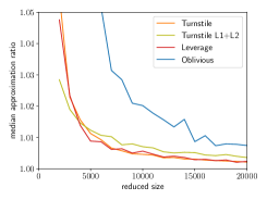
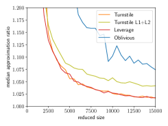
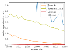
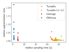
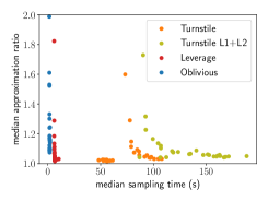
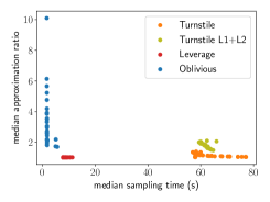
Logistic Regression
     CoverType      WebSpam      KddCup Approx. Ratio Sampling Time Total Time

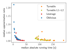
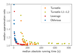
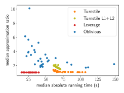
Figure 2: Comparison of the approximation ratios and running times for logistic regression on various real-world datasets. The new turnstile data stream sampler for $p=1$ (orange) and a mixture $p=1,q=2$ (lime) is compared to plain leverage score sampling (red), and to plain oblivious sketching (blue). The plots indicate the median of approximation ratios taken over 21 repetitions for each reduced size. Best viewed in colors, lower is better.

I.6 Experiments for $\ell_{1}$ regression

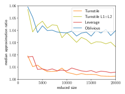
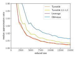
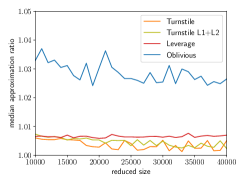
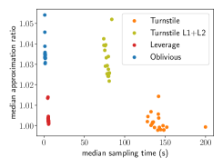
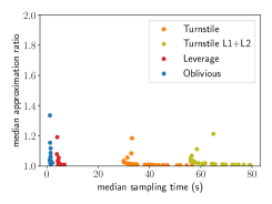
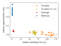
Linear $\ell_{1}$ Regression
     CoverType      WebSpam      KddCup Approx. Ratio Sampling Time Total Time

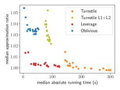
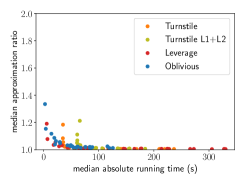
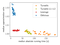
Figure 3: Comparison of the approximation ratios and running times for $\ell_{1}$ regression on various real-world datasets. The new turnstile data stream sampler for $p=1$ (orange) and a mixture $p=1,q=2$ (lime) is compared to plain leverage score sampling (red), and to plain oblivious sketching (blue). The plots indicate the median of approximation ratios taken over 21 repetitions for each reduced size. Best viewed in colors, lower is better.

I.7 Experiments for $\ell_{1.5}$ regression

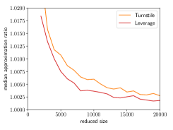
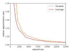
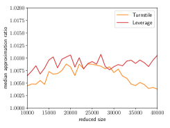
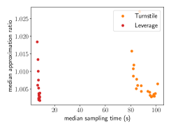
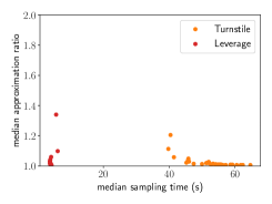
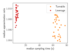
Linear $\ell_{1.5}$ Regression
     CoverType      WebSpam      KddCup Approx. Ratio Sampling Time Total Time

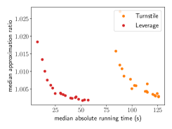
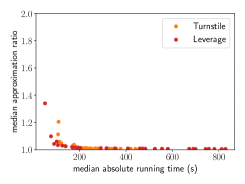
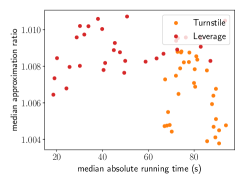
Figure 4: Comparison of the approximation ratios and running times for $\ell_{1.5}$ regression on various real-world datasets. The new turnstile data stream sampler for $p=1.5$ (orange) is compared to plain leverage score sampling for $p=1.5$ (red). The plots indicate the median of approximation ratios taken over 21 repetitions for each reduced size. Best viewed in colors, lower is better.

References

- Ai et al., (2016) Ai, Y., Hu, W., Li, Y., and Woodruff, D. P. (2016). New characterizations in turnstile streams with applications. In 31st Conference on Computational Complexity (CCC), pages 20:1–20:22.
- Alon et al., (1986) Alon, N., Babai, L., and Itai, A. (1986). A fast and simple randomized parallel algorithm for the maximal independent set problem. J. Algorithms, 7(4):567–583.
- Alon et al., (1999) Alon, N., Matias, Y., and Szegedy, M. (1999). The space complexity of approximating the frequency moments. J. Comput. Syst. Sci., 58(1):137–147.
- Andoni et al., (2011) Andoni, A., Krauthgamer, R., and Onak, K. (2011). Streaming algorithms via precision sampling. In IEEE 52nd Annual Symposium on Foundations of Computer Science (FOCS), pages 363–372.
- Andoni et al., (2013) Andoni, A., Nguyên, H. L., Polyanskiy, Y., and Wu, Y. (2013). Tight lower bound for linear sketches of moments. In Proceedings of the 40th International Colloquium on Automata, Languages, and Programming (ICALP), pages 25–32.
- Bentley and Saxe, (1980) Bentley, J. L. and Saxe, J. B. (1980). Decomposable searching problems I: Static-to-dynamic transformation. J. Algorithms, 1(4):301–358.
- Bhaskara et al., (2023) Bhaskara, A., Mahabadi, S., and Vakilian, A. (2023). Tight bounds for volumetric spanners and applications. In Advances in Neural Information Processing Systems 36 (NeurIPS).
- Braverman et al., (2017) Braverman, V., Frahling, G., Lang, H., Sohler, C., and Yang, L. F. (2017). Clustering high dimensional dynamic data streams. In Proceedings of the 34th International Conference on Machine Learning (ICML), pages 576–585.
- Charikar et al., (2004) Charikar, M., Chen, K. C., and Farach-Colton, M. (2004). Finding frequent items in data streams. Theor. Comput. Sci., 312(1):3–15.
- Chhaya et al., (2020) Chhaya, R., Choudhari, J., Dasgupta, A., and Shit, S. (2020). Streaming coresets for symmetric tensor factorization. In Proceedings of the 37th International Conference on Machine Learning (ICML), pages 1855–1865.
- Clarkson and Woodruff, (2017) Clarkson, K. L. and Woodruff, D. P. (2017). Low-rank approximation and regression in input sparsity time. Journal of the ACM, 63(6):1–45.
- Cohen et al., (2020) Cohen, M. B., Musco, C., and Pachocki, J. (2020). Online row sampling. Theory Comput., 16:1–25.
- Cohen and Peng, (2015) Cohen, M. B. and Peng, R. (2015). row sampling by Lewis weights. In Proceedings of the Forty-Seventh Annual ACM on Symposium on Theory of Computing (STOC), pages 183–192.
- Cohen-Addad et al., (2023) Cohen-Addad, V., Woodruff, D. P., and Zhou, S. (2023). Streaming euclidean k-median and k-means with o(log n) space. In IEEE 64th Annual Symposium on Foundations of Computer Science (FOCS), pages 883–908.
- Cormode and Jowhari, (2019) Cormode, G. and Jowhari, H. (2019). samplers and their applications: A survey. ACM Comput. Surv., 52(1):16:1–16:31.
- Dasgupta et al., (2009) Dasgupta, A., Drineas, P., Harb, B., Kumar, R., and Mahoney, M. W. (2009). Sampling algorithms and coresets for regression. SIAM J. Comput., 38(5):2060–2078.
- Dietzfelbinger, (1996) Dietzfelbinger, M. (1996). Universal hashing and k-wise independent random variables via integer arithmetic without primes. In Proc. of the 13th Annual Symposium on Theoretical Aspects of Computer Science (STACS), pages 569–580.
- Drineas et al., (2012) Drineas, P., Magdon-Ismail, M., Mahoney, M. W., and Woodruff, D. P. (2012). Fast approximation of matrix coherence and statistical leverage. J. Mach. Learn. Res., 13:3475–3506.
- Drineas et al., (2006) Drineas, P., Mahoney, M. W., and Muthukrishnan, S. (2006). Sampling algorithms for regression and applications. In Proceedings of the 17th Annual ACM-SIAM Symposium on Discrete Algorithms (SODA), pages 1127–1136.
- Feldman et al., (2020) Feldman, D., Schmidt, M., and Sohler, C. (2020). Turning Big Data into tiny data: Constant-size coresets for k-means, pca, and projective clustering. SIAM J. Comput., 49(3):601–657.
- Frahling et al., (2008) Frahling, G., Indyk, P., and Sohler, C. (2008). Sampling in dynamic data streams and applications. Int. J. Comput. Geom. Appl., 18(1/2):3–28.
- Frahling and Sohler, (2005) Frahling, G. and Sohler, C. (2005). Coresets in dynamic geometric data streams. In Proceedings of the 37th Annual ACM Symposium on Theory of Computing (STOC), pages 209–217.
- Frick et al., (2024) Frick, S., Krivosija, A., and Munteanu, A. (2024). Scalable learning of item response theory models. In International Conference on Artificial Intelligence and Statistics (AISTATS), pages 1234–1242.
- Geppert et al., (2020) Geppert, L. N., Ickstadt, K., Munteanu, A., and Sohler, C. (2020). Streaming statistical models via Merge & Reduce. Int. J. Data Sci. Anal., 10(4):331–347.
- Haagerup, (1981) Haagerup, U. (1981). The best constants in the Khintchine inequality. Studia Mathematica, 70(3):231–283.
- Indyk, (2006) Indyk, P. (2006). Stable distributions, pseudorandom generators, embeddings, and data stream computation. J. ACM, 53(3):307–323.
- Jayaram and Woodruff, (2021) Jayaram, R. and Woodruff, D. P. (2021). Perfect sampling in a data stream. SIAM J. Comput., 50(2):382–439.
- Jayaram et al., (2022) Jayaram, R., Woodruff, D. P., and Zhou, S. (2022). Truly perfect samplers for data streams and sliding windows. In International Conference on Management of Data (PODS), pages 29–40.
- Jowhari et al., (2011) Jowhari, H., Saglam, M., and Tardos, G. (2011). Tight bounds for samplers, finding duplicates in streams, and related problems. In Proceedings of the 30th ACM SIGMOD-SIGACT-SIGART Symposium on Principles of Database Systems (PODS), pages 49–58.
- Langberg and Schulman, (2010) Langberg, M. and Schulman, L. J. (2010). Universal -approximators for integrals. In Proceedings of the Twenty-First Annual ACM-SIAM Symposium on Discrete Algorithms (SODA), pages 598–607.
- Li et al., (2014) Li, Y., Nguyen, H. L., and Woodruff, D. P. (2014). Turnstile streaming algorithms might as well be linear sketches. In Symposium on Theory of Computing (STOC), pages 174–183.
- Li and Woodruff, (2016) Li, Y. and Woodruff, D. P. (2016). On approximating functions of the singular values in a stream. In Proceedings of the 48th Annual ACM SIGACT Symposium on Theory of Computing (STOC), pages 726–739.
- Li et al., (2021) Li, Y., Woodruff, D. P., and Yasuda, T. (2021). Exponentially improved dimensionality reduction for : Subspace embeddings and independence testing. In Conference on Learning Theory (COLT), pages 3111–3195.
- Mahabadi et al., (2020) Mahabadi, S., Razenshteyn, I. P., Woodruff, D. P., and Zhou, S. (2020). Non-adaptive adaptive sampling on turnstile streams. In Proccedings of the 52nd Annual ACM SIGACT Symposium on Theory of Computing (STOC), pages 1251–1264.
- Mai et al., (2023) Mai, T., Munteanu, A., Musco, C., Rao, A. B., Schwiegelshohn, C., and Woodruff, D. P. (2023). Optimal sketching bounds for sparse linear regression. In Proceedings of the 26th International Conference on Artificial Intelligence and Statistics (AISTATS).
- Mai et al., (2021) Mai, T., Musco, C., and Rao, A. (2021). Coresets for classification - simplified and strengthened. In Advances in Neural Information Processing Systems 34 (NeurIPS), pages 11643–11654.
- Molina et al., (2018) Molina, A., Munteanu, A., and Kersting, K. (2018). Core dependency networks. In Proceedings of the Thirty-Second AAAI Conference on Artificial Intelligence (AAAI), pages 3820–3827.
- Monemizadeh and Woodruff, (2010) Monemizadeh, M. and Woodruff, D. P. (2010). 1-pass relative-error -sampling with applications. In Proceedings of the Twenty-First Annual ACM-SIAM Symposium on Discrete Algorithms (SODA), pages 1143–1160.
- Munteanu, (2023) Munteanu, A. (2023). Coresets and sketches for regression problems on data streams and distributed data. In Machine Learning under Resource Constraints, Volume 1 - Fundamentals, pages 85–98. De Gruyter, Berlin, Boston.
- Munteanu and Omlor, (2024) Munteanu, A. and Omlor, S. (2024). Optimal bounds for sensitivity sampling via augmentation. In Proceedings of the 41st International Conference on Machine Learning (ICML).
- Munteanu et al., (2022) Munteanu, A., Omlor, S., and Peters, C. (2022). -Generalized probit regression and scalable maximum likelihood estimation via sketching and coresets. In Proceedings of the 25th International Conference on Artificial Intelligence and Statistics (AISTATS), pages 2073–2100.
- Munteanu et al., (2021) Munteanu, A., Omlor, S., and Woodruff, D. P. (2021). Oblivious sketching for logistic regression. In Proceedings of the 38th International Conference on Machine Learning (ICML), pages 7861–7871.
- Munteanu et al., (2023) Munteanu, A., Omlor, S., and Woodruff, D. P. (2023). Almost linear constant-factor sketching for and logistic regression. In The Eleventh International Conference on Learning Representations, (ICLR).
- Munteanu and Schwiegelshohn, (2018) Munteanu, A. and Schwiegelshohn, C. (2018). Coresets-methods and history: A theoreticians design pattern for approximation and streaming algorithms. Künstliche Intell., 32(1):37–53.
- Munteanu et al., (2018) Munteanu, A., Schwiegelshohn, C., Sohler, C., and Woodruff, D. P. (2018). On coresets for logistic regression. In Advances in Neural Information Processing Systems 31 (NeurIPS), pages 6562–6571.
- Muthukrishnan, (2005) Muthukrishnan, S. (2005). Data streams: Algorithms and applications. Found. Trends Theor. Comput. Sci., 1(2).
- Nisan, (1992) Nisan, N. (1992). Pseudorandom generators for space-bounded computation. Comb., 12(4):449–461.
- Phillips, (2017) Phillips, J. M. (2017). Coresets and sketches. In Handbook of Discrete and Computational Geometry, pages 1269–1288. Chapman and Hall/CRC, 3rd edition.
- Rusu and Dobra, (2007) Rusu, F. and Dobra, A. (2007). Pseudo-random number generation for sketch-based estimations. ACM Transactions on Database Systems, 32(2):1–48.
- Sohler and Woodruff, (2011) Sohler, C. and Woodruff, D. P. (2011). Subspace embeddings for the -norm with applications. In Proceedings of the 43rd ACM Symposium on Theory of Computing (STOC), pages 755–764.
- Wang and Woodruff, (2022) Wang, R. and Woodruff, D. P. (2022). Tight bounds for oblivious subspace embeddings. ACM Trans. Algorithms, 18(1):8:1–8:32.
- Woodruff, (2014) Woodruff, D. P. (2014). Sketching as a tool for numerical linear algebra. Found. Trends Theor. Comput. Sci., 10(1-2):1–157.
- (53) Woodruff, D. P. and Yasuda, T. (2023a). New subset selection algorithms for low rank approximation: Offline and online. In Proceedings of the 55th Annual ACM Symposium on Theory of Computing (STOC), pages 1802–1813.
- (54) Woodruff, D. P. and Yasuda, T. (2023b). Online Lewis weight sampling. In Proceedings of the 2023 ACM-SIAM Symposium on Discrete Algorithms (SODA), pages 4622–4666.
- (55) Woodruff, D. P. and Yasuda, T. (2023c). Sharper bounds for sensitivity sampling. In International Conference on Machine Learning (ICML), pages 37238–37272.
- Woodruff and Zhang, (2013) Woodruff, D. P. and Zhang, Q. (2013). Subspace embeddings and -regression using exponential random variables. In The 26th Annual Conference on Learning Theory (COLT), pages 546–567.