Magnetic ground state of monolayer CeI₂: occupation matrix control and DFT+U calculations

Abstract

The magnetic ground state is crucial for the applications of the two-dimension magnets as it decides fundamental magnetic properties of the material, such as magnetic order, magnetic transition temperature, and low-energy excitation of the spin waves. However, the simulations for magnetism of local-electron systems are challenging due to the existence of metastable states. In this study, occupation matrix control (OMC) and density functional theoryplus Hubbard $U$ calculations are applied to investigate the magnetic ground state of monolayer CeI₂. Following the predicted ferrimagnetic (FM) order, the FM ground state and the FM metastable states are identified and found to have different values of the magnetic parameters. Based on the calculated magnetic parameters of the FM ground state, the Curie temperature is estimated to be $128$ K for monolayer CeI₂. When spin-orbit coupling (SOC) is considered, the FM ground state is further confirmed to contain both off-plane and in-plane components of magnetization. SOC is shown to be essential for reasonably describing not only magnetic anisotropy but also local electronic orbital state of monolayer CeI₂.

I Introduction

The two-dimension(2D) magnetsexhibit magnificent potential in spintronic devices and magnetic storage devices due to their unique properties and the nanoscale size. Although Mermin-Wagner theorem Mermin denies the possibility of long-range magnetic order in 2D systems at non-zero temperature, a series of experimental studies Jiang2021 ; Huang2017 ; Tian2019 ; Cai2019 ; Zhang2019 ; Banerjee2017 ; Zhou2019 ; Bonilla2018 ; Li2018 ; Hara2018 ; Gong2017 ; Wang2016 ; Kim2019 ; Flem1982 ; Fei2018 ; May2019 have confirmedthe presence of magnetic orders in 2D materials. These findings encourage people to further explore 2D magnetic materials with superior properties, such as robust dynamic stability, high magnetic transition temperature, and unique magnetic anisotropy.

The magnetic ground state (GS) of a 2D material issignificant. It not only dominates the behaviour about magnetism at low temperature, but decides the low-energy excitation of the spin waves at finite temperature. For magnetic crystals, a comprehensive description of the magnetic GS should contain the information of two aspects: the specific magnetic structure and the electronic states of the magnetic sites. For the former part, Spin-polarized scanning tunneling microscope (SP-STM), Ramam spectroscopy, and the observation of anomalous Hall effect have been adopted to examine the magnetic order of 2D magnetic insulators and 2D magnetic metals Huang2017 ; Gong2017 ; May2019 ; Lee2016 ; Tian2016 ; Deng2018 . For the latter part, x-ray magnetic circular dichroism (XMCD) and x-ray magnetic linear dichroism(XMLD) are two techniques which help to obtain the local electronic configuration Liu2016 ; Laan1999 . Nonetheless, exploring magnetic ground states of 2D materials experimentally is still challenging. The limitations include the acquirement of high quality samples, strict experimental conditions, and even expensive costs on economy and time. From this point of view, exploring 2D magnetic materials by using density functional theory (DFT) calculations is another feasible scheme. The DFT tool gives the prediction of the magnetic ground state without synthesizing actual samples. It has been applied to study a series of 2D magnetic materials such as layered $\alpha$-RuCl₃, VSe(Te)₂, CrGe(Si)Te₃, etc. Sarikurt2018 ; Kim20161 ; Sandilands2015 ; Li2014 ; Ataca2012 ; Chen2020 ; Fuh2016 ; Pan2014 ; Kan2014 ; Lin2017 ; Lin2016 For 2D CrI₃ and CrBr₃, DFT calculations give quite consistent prediction of magnetic features with the experiments, including the magnetic structure and Curie temperature ($T_{\text{C}}$) Wang20162 ; Zhang2015 ; Liu20162 ; Jiang20212 . With the assistance of DFT calculations, the studying progress of 2D magnetic materials has been accelerated significantly.

In 2D magnetic insulators and semiconductors, the spin moments are commonly contributed by polarized electrons from partially filled $d$ or f atomic shells. These electrons are localized around the lattice sites and need extra corrections for strong electronic correlation. Therefore, the density functional theory plus Hubbard $U$ (DFT+U) scheme Liechtenstein ; Dudarev is widely applied to give reasonable electronic structures of the correlated systems. In fact, the conventional DFT+U computational scheme faces challenges in locating the ground state of the localized electrons due to the presence of metastable states, especially when the d and f shells are less filled. In other words, although a specific magnetic ordered state can be determined by DFT+U calculations, however, the obtained electronic state of the localized electrons may be not identical for different researchers. This phenomenon has appeared in the DFT+U studies of Ti-based systems Watson , Ce-based systems Watson ; Shick , U-based systems Miskowiec ; Dorado ; Dorado1 ; Dorado2 ; Matthew ; Claisse , cubic fluorite PuO₂ Jomard ; Hou2022 , etc., and the metastable states can originate from 3$d$, 4$f$, or 5$f$ localized electrons (not found in 4$d$ or 5$d$ electronic systems yet, to our knowledge). Moreover, these works have also shown that the occurrence of trapping into metastable states is not relevant to the form of adopted exchange-correlation functional. Local density approximation (LDA) Shick , generalized gradient approximation (GGA) Watson ; Miskowiec ; Dorado ; Dorado1 , strongly constrained appropriate normed (SCAN) type meta-GGA Hou2022 , and HSE06 type hybrid Jollet ; Ratcliff functionals have been adopted in the studies but this accident still happens constantly. To solve the problem, a few techniques have been developed including U-ramping Claisse ; Meredig , quasi-annealing Geng , occupation matrix control (OMC) Watson ; Dorado ; Claisse ; Amadon ; Zhou2011 ; Zhou2022 , DFT+DMFT Amadon2012 and even the combination of them Rabone . These techniques help to reduce the probability of trapping into metastable states to some extent. However, it remains an open question as to how the ground state of the localized electrons can be accurately obtained.

Recently, the monolayer CeI₂ was predicted to be an in-plane ferrimagnetic (FM) semiconductor with a high $T_{\text{C}}$ of $374$ K by DFT+U calculations Sheng . The dynamic stability of the monolayer CeI₂ was supported by both phonon calculations and a molecular dynamics simulation at room temperature. In the monolayer CeI₂, two 6s electrons of the Ce atom move away to form the Ce-I bond, leaving a $4f^{1}5d^{1}$ electronic configuration for the Ce²⁺ ion. According to above analysis, a number of metastable states originated from the highly localized $4f$ electrons should be expected. Owing to the importance for both basic physics and potential applications, it is necessary to provide a systematic analysis of the magnetic GS of monolayer CeI₂.

In this study, we perform DFT+U calculations combined with OMC to investigate the magnetic GS of monolayer CeI₂. The magnetic structure is once again confirmed to be FM. The FM GS as well as twenty-three FM metastable states of monolayer CeI2 with different local electronic states are identified. Our results show that the calculated isotropy exchange parameter and magnetic anisotropy energy are distinguishable for the GS and metastable states. Based on the exchange parameters of the magnetic GS, the $T_{\text{C}}$ is estimated to be about $128$ K by using Monte Carlo simulations. To reasonably analyze the contributions to the total energies, the Coulomb potential energies of the 4f electron with different occupied electronic orbitals in the crystal field are discussed. Furthermore, we take spin-orbit coupling (SOC) into consideration. The magnetic structure of monolayer CeI₂ then becomes FM with both in-plane and off-plane components of magnetic moments and the easy axis of magnetization is coupled with the crystal structure. The single Ce-$4f$ electron occupies another distinguishable electronic orbital compared to the situation without SOC, which illustrates that SOC is essential to describe the magnetic GS of monolayer CeI₂. A fully off-plane FM state is confirmed to be a metastable state of monolayer CeI₂ whose total energy is just slightly higher than the magnetic GS. We anticipate that achieving saturation magnetization in the off-plane direction for monolayer CeI₂ is feasible under appropriate external conditions.

II Computational Methods

The DFT+U calculations are carried out by employing the Vienna abinitiosimulation package (VASP) code Kresse . OMC is implemented by applying the patch of Allen et al. tailored for VASP Watson . The adopted atomic pseudo potentials are constructed by the project augmented wave (PAW) method Blochl ; Kresse2 ; Blochl2 . The cut-off energy of the plane wave bases is set to $600$ eV. The first Brillouin Zone is sampled by a $\Gamma$-center $11\times 11\times 1$ $k$-point mesh. The convergence of both cut-off energy and $k$-point mesh has been carefully examined. The crystal structures are relaxed until the Feynman-Hellman force on each atom is smaller than $0.005$ eV/Å The optimizing of the charge density is ended when the energy difference is smaller than $10^{-6}$ eV between the current two steps of the iteration. We make use of the DFT+U method of Dudarev et al. Dudarev with a form of

$$E_{\text{DFT+U}}=E_{\text{DFT}}+\frac{U-J}{2}\sum_{\sigma}\left[\left(\sum_{m_{1}}n_{m_{1},m_{1}}^{\sigma}\right)-\left(\sum_{m_{1},m_{2}}n_{m_{1},m_{2}}^{\sigma}n_{m_{2},m_{1}}^{\sigma}\right)\right],$$ (1)

where $n_{m_{1},m_{2}}^{\sigma}$ is the matrix element of the occupation matrix with spin $\mathit{\sigma}$. The standard DFT part here is handled by the Perdew-Burke-Ernzerhof (PBE) type GGA exchange-correlation functional Perdew The Hubbard $U$ and Hund $J$ for the Ce-$4f$ electron are set to be $7.47$ eV and $0.99$ eV, respectively, which have been applied in previous study Sheng ; Larson . To be cautious, a discussion is also made to demonstrate the rationality of the $U$ parameter (see Section B of the Supporting information). Based on the calculated Bloch states by plane waves bases, Wannier90 code Mostofi is used to construct the tight-binding Hamiltonian. TB2J code He is used to calculate the Green’s function and then the isotropic exchange parameter for magnetic properties is obtained. The $T_{\text{C}}$ is gained by Monte Carlo simulations based on the heat bath algorithms Miyatake . The visualizations of the crystal structure and spin densities in this work is achieved by VESTA Momma . The VASPKIT code is used to process the data of the DFT calculations Wang2021 .

III OMC of the $4f^{1}$ electronic state

A quantum state of a single electron can be express as a linear combination of a group of complete and orthogonal bases in the Hilbert space. In the limitation of localized electrons of an isolated atom, the dimension of the space is equal to $2l+1$, where $l$ is the angular quantum number of that electron. In monolayer CeI₂, $l$ is no longer a good quantum number for the $5d$ electron of Ce²⁺ since the $5d$ electron is not well localized. Additionally, the delocalized $5d$ electron has a more plane-wave-like charge density rather than the atomic-orbital-like charge density of the $4f$ electron. Hence only the $4f$ electron is accompanied by high risks of falling into metastable states in DFT+U calculations. Its electronic orbital requires careful control and observation.

The occupation matrix is the density matrix in particle-number representation and a $14\times 14$ occupation matrix is sufficient to represent the electronic state of the single $4f$ electron exactly. Here the general set of 4f atomic orbitals is used as the bases, which are $f_{y(3x^{2}-y^{2})^{\uparrow}}$, $f_{xyz^{\uparrow}}$, $f_{yz^{2\uparrow}}$, $f_{z^{3\uparrow}}$, $f_{xz^{2\uparrow}}$, $f_{z(x^{2}-y^{2})^{\uparrow}}$, $f_{x(x^{2}-3y^{2})^{\uparrow}}$, $f_{y(3x^{2}-y^{2})^{\downarrow}}$, $f_{xyz^{\downarrow}}$, $f_{yz^{2\downarrow}}$, $f_{z^{3\downarrow}}$, $f_{xz^{2\downarrow}}$, $f_{z(x^{2}-y^{2})^{\downarrow}}$, and $f_{x(x^{2}-3y^{2})^{\downarrow}}$, respectively. The spin-quantization axis is chosen to be along $z$ direction of the Cartesian coordinate system. We firstly do not take SOC into consideration. Since there is only one localized electron in the $4f$ shell of Ce²⁺, any quantum state of the single electron with both spin up and spin down components is unphysical. We thus neglect the spin index and a quantum state of the single $4f$ electron can be written as

$$\psi_{4f}=c_{1}f_{y(3x^{2}-y^{2})}+c_{2}f_{xyz}+c_{3}f_{yz^{2}}+c_{4}f_{z^{2}}+c_{5}f_{xz^{2}}+c_{6}f_{z(x^{2}-y^{2})}+c_{7}f_{x\left(x^{2}-3y^{2}\right)},$$ (2)

where $c_{i}$ ($i=1,2,\cdots,7$) is the complex expansion coefficient of the basis. There should be

$$\sum_{i}c_{i}=1.$$ (3)

For simplicity, we mark the quantum state as ($c_{1}$, $c_{2}$, $c_{3}$, $c_{4}$, $c_{5}$, $c_{6}$, $c_{7}$) for the following part of this paper. The eigenvectors and eigenvalues of the occupation matrix are actually quantum states and the corresponding occupation numbers, respectively.

An OMC procedure is to set a initial occupation matrix artificially for the localized electrons in the DFT+U calculations. The initial occupation matrix has also been called the starting point Zhou2022 . Different starting points may access to different final states of the localized electrons. In our calculations, we make our starting points for the Ce-$4f$ electron all diagonal with a average occupation on several orbital bases. The down spin block and the two off-diagonal blocks of the $14\times 14$ occupation matrix are null matrices. The up spin block of the occupation matrix has a form of

$$\left(\begin{array}[c]{cccc}a_{1}&0&\cdots&0\\ 0&a_{2}&\cdots&0\\ \cdots&\cdots&\cdots&\cdots\\ 0&0&\cdots&a_{7}\end{array}\right)$$ (4)

with

$$a_{i}=0\text{, or }\frac{1}{n}\text{ (}i,n=1,2,\cdots,7\text{),}$$ (5)

where $n$ is the number of orbital bases whose occupation number is non-zero. The trace of the up spin block is the number of occupying electrons, which is equal to $1$ for the Ce-$4f$ shell here. Hence there is

$$\sum_{i}a_{i}=1.$$ (6)

Based on Eqs. (4)-(6), we have $\sum\nolimits_{i=1}^{7}C_{7}^{i}=127$ different starting points for the DFT+U calculations. After the self-consistence iteration processes based on different starting points, we obtain twenty-four final states of monolayer CeI₂, whose $4f$ electronic states are different with each other. A detailed discussion of the OMC procedure for the SOC situation is provided in Section C of the Supporting information.

IV Magnetic properties of the GS and metastable states

The optimized crystal structure of monolayer CeI₂ is shown in Fig. 1(a). Each Ce²⁺ ion is surrounded by six nearest I^- ions which form a regular triangle prism (RTP). The distance between two nearest Ce²⁺ ions is $4.28$ Å which makes the direct exchange from different Ce sites negligible. The main reason that causes the magnetic order should be the superexchange interaction mediated by I-$p$ electrons. Since both Ce-$4f$ and Ce-$5d$ electrons contribute to the superexchange interaction, the total inter-site exchange strength can be decomposed to $J^{d-d}$, $J^{d-f}$, and $J^{f-f}$, as shown in Fig. 1(b). These are the exchange parameter between $5d$ shell and $5d$ shell, $5d$ shell and $4f$ shell, and $4f$ shell and $4f$ shell from different sites, respectively. Meanwhile, with the help of coordinated I^- ions, the $d-f$ hybridization on each Ce site should be considered. This on-site $d-f$ exchange parameter is denoted by $J^{\text{site}}$, as shown in Fig. 1(b). For the inter-site exchange parameters, we only consider the first nearest exchange parameter $J_{1}$ and second nearest exchange parameter $J_{2}$ as shown in Fig. 1(a). Hence the total Hamiltonian of CeI₂ can be express as

$$\hat{H}_{\text{tot}}=\delta-J_{1}\sum_{\left\langle i,j\right\rangle}\vec{S}_{i}\cdot\vec{S}_{j}-J_{2}\sum_{\left\langle\left\langle i,j\right\rangle\right\rangle}\vec{S}_{i}\cdot\vec{S}_{j}-J^{\text{site}}\sum_{i}\vec{S}_{i}^{d}\cdot\vec{S}_{i}^{f}$$ (7)

with

$$J_{1}=J^{d-d}+J^{d-f}+J^{f-f},$$ (8)

where $\mathit{\delta}$ is the spin-independent part of the total energy. $i$ and $j$ denote different sites in the unit cell.

All the following discussions for monolayer CeI₂ are based on the fact that the magnetic structure of the GS is FM no matter which orbital the localized electron is occupying. This feature of CeI₂ has been verified by our calculations for the total energy and exchange parameters as introduced in the following section. With OMC applied, the relative energies of the GS and the metastable states of FM CeI₂ are listed in Table I. It is noteworthy that the FM state studied by the former study Sheng is confirmed to be a metastable state (S₂₀) in our work.

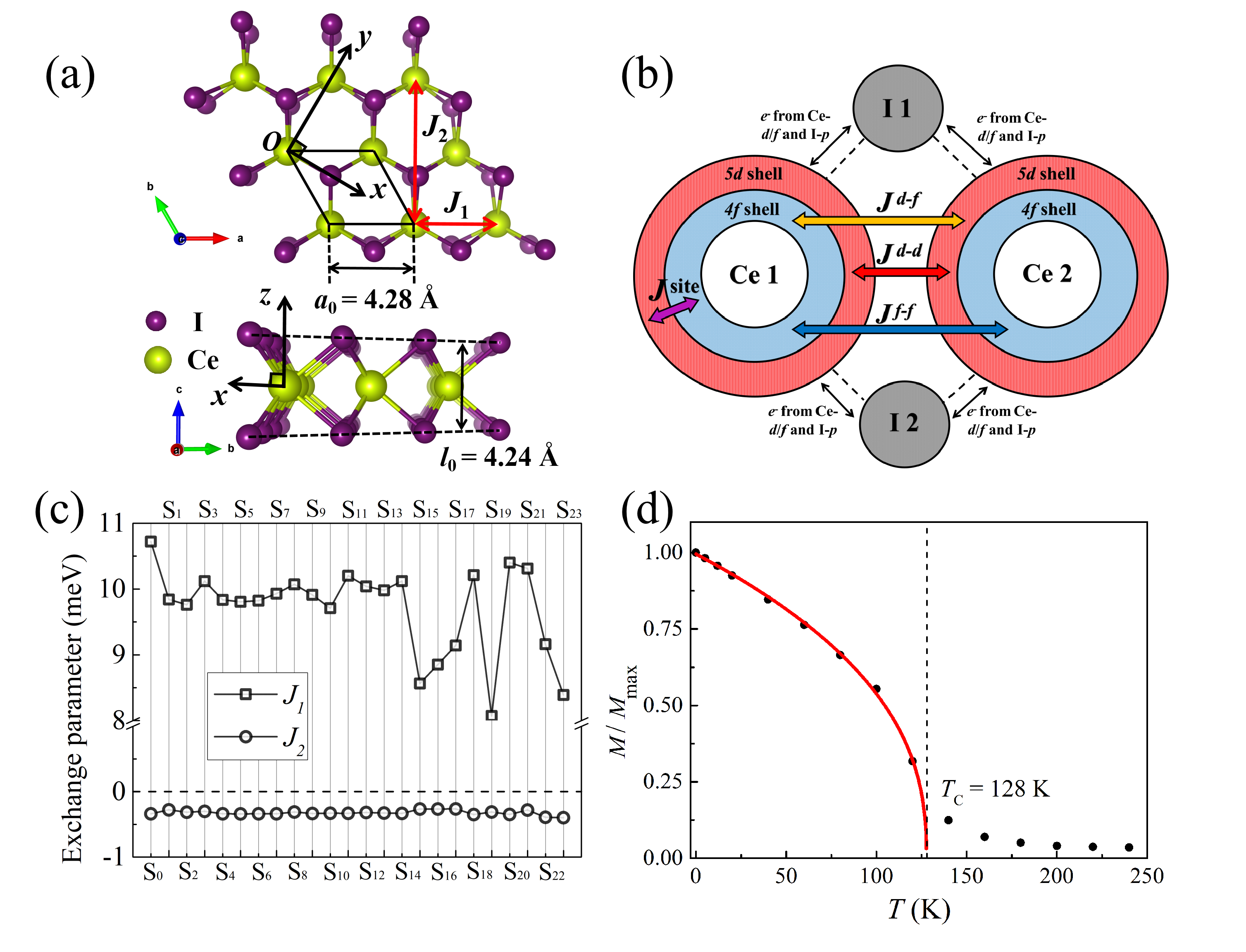
Figure 1: (Color online) (a) The optimized crystal structure of monolayer CeI₂. $a_{0}$ and $l_{0}$ are the lattice parameter and thickness of monolayer CeI₂. (b) The components ($J^{d-d}$, $J^{d-f}$, and $J^{f-f}$) of the first nearest inter-site exchange parameter and the on-site $d-f$ exchange parameter ($J^{\text{site}}$) in monolayer CeI₂. (c) The values of first nearest exchange parameter $J_{1}$ and second nearest exchange parameter $J_{2}$ for the GS and metastable states. (d) The temperature dependent magnetization intensity of monolayer CeI₂ with a quenching at $128$ K predicted by Monte-Carlo simulations.

By using a model Hamiltonian of spin interactions like Eq. (7) in combination with the DFT total energies of different magnetic structures, one can fit the values of the exchange parameters. However, this scheme is invalid for monolayer CeI₂ because the exchange parameter is not identical for different magnetic structures. A detailed discussion about it is given in Section D of the Supporting information. Here, we make use of the obtained Bloch states by a self-consistence calculation to construct tight-binding Hamiltonian and calculate the exchange parameter by using Green’s function method He . The values of $J_{1}$ and $J_{2}$ for monolayer CeI₂ with different local electronic states are shown in Fig. 1(c). One can find that $J_{1}$ is always positive and $J_{2}$ is always negative for all the states. The absolute value of $J_{1}$ is far greater than $J_{2}$, which favors FM order of monolayer CeI₂. Note that $J_{1}$ is quite sensitive to the $4f$ electronic states.

The exchange parameters of the ground state S₀ are used to simulate the $T_{\text{C}}$ of monolayer CeI₂. There are $J_{1}=10.7$ meV and $J_{2}=-0.34$ meV. Monte-Carlo method is used and $T_{\text{C}}$ is estimated to be about $128$ K as shown in Fig. 1(d). It is important to note that the presence of metastable states of monolayer CeI₂ can lead to different values of the inter-site exchange parameters, potentially affecting the reliability of the predicted $T_{\text{C}}$ for the material. Therefore, it is also recommended to exclude the metastable states before conducting further calculations for other local-electron systems, in addition to monolayer CeI₂.

Table 1: The 1${}^{\text{st}}$ column lists the GS (S₀) and the metastable states (S₁-S₂₃). The 2${}^{\text{nd}}$ column gives the DFT total energies of all the FM states relative to the GS denoted as $\Delta E$ (in unit of meV). The 3${}^{\text{rd}}$ column shows the specific representations of the calculated $4f^{1}$ states with $f_{y(3x^{2}-y^{2})}$, $f_{xyz}$, $f_{yz^{2}}$, $f_{z^{3}}$, $f_{xz^{2}}$, $f_{z(x^{2}-y^{2})}$, and $f_{x(x^{2}-3y^{2})}$ as bases. The 4${}^{\text{th}}$ to the 6${}^{\text{th}}$ columns give the relative energies of $x$, $y$, and $z$ directions of spin polarization for each state (in unit of $\mu$eV). The 7${}^{\text{th}}$ to the 10${}^{\text{th}}$ columns give the values of $J^{\text{site}}$, $J^{d-d}$, $J^{d-f}$, and $J^{f-f}$ for each state (in unit of meV).

	$\Delta E$	$4f^{1}$ electronic state	$x$	$y$	$z$	$J^{\text{site}}$	$J^{d-d}$	$J^{d-f}$	$J^{f-f}$
S0	$0$	$(0.66,0,0,-0.74,0,0,0)$	$0$	$0$	$393$	$116.1$	$10.2$	$0.30$	$0.22$
S1	$4.4$	$(0,0,0,-0.74,0,0,0.66)$	$0$	$0$	$381$	$113.9$	$9.18$	$0.38$	$0.28$
S2	$5.0$	$(0.62,0,0.4,0.6,0,-0.3,0)$	$0$	$0$	$409$	$104.3$	$9.10$	$0.49$	$0.17$
S3	$5.0$	$(0.38,0.1,0.33,-0.61,0.29,0,-0.53)$	$0$	$6$	$406$	$107.4$	$8.60$	$1.42$	$0.10$
S4	$6.6$	$(0.62,0,-0.79,0,0,0,0)$	$0$	$24$	$461$	$97.3$	$9.04$	$0.56$	$0.24$
S5	$6.6$	$(0.61,0,0.38,0,-0.69,0,0)$	$9$	$0$	$455$	$97.3$	$9.58$	$0.20$	$0.03$
S6	$7.3$	$(0.54,0,0.28,0,0.73,0,0.29)$	$27$	$0$	$460$	$96.9$	$9.22$	$0.40$	$0.21$
S7	$7.6$	$(0.5,0,-0.77,0,0.16,0,-0.34)$	$0$	$25$	$458$	$96.7$	$9.33$	$0.50$	$0.10$
S8	$7.6$	$(0.24,0.1,0.5,-0.45,0.37,0,-0.58)$	$0$	$13$	$425$	$101.6$	$8.78$	$1.14$	$0.15$
S9	$8.3$	$(0.43,0,-0.76,0,0.2,0,-0.43)$	$0$	$25$	$456$	$96.3$	$9.22$	$0.70$	$0.01$
S10	$8.4$	$(0.42,0,0.19,0,-0.76,0,-0.45)$	$17$	$0$	$462$	$96.2$	$8.34$	$1.24$	$0.13$
S11	$8.5$	$(0.4,0,0.57,0,0.54,0,-0.47)$	$0$	$12$	$449$	$96.2$	$8.70$	$1.32$	$0.18$
S12	$9.9$	$(0,0,0,0,0.79,0,0.61)$	$46$	$0$	$460$	$95.4$	$8.86$	$0.67$	$0.51$
S13	$9.9$	$(0,0,-0.68,0,-0.4,0,0.61)$	$0$	$23$	$450$	$95.4$	$9.16$	$0.60$	$0.22$
S14	$24.1$	$(0.33,0,0.6,0,-0.52,0,0.52)$	$0$	$15$	$449$	$80.8$	$8.25$	$1.49$	$0.38$
S15	$33.3$	$(0,1,0,0,0,0,0)$	$44$	$0$	$428$	$49.0$	$7.83$	$0.50$	$0.24$
S16	$33.3$	$(0,0,0,0,0,1,0)$	$0$	$43$	$427$	$49.0$	$7.99$	$0.60$	$0.26$
S17	$33.3$	$(0,-0.92,0,0,0,0.4,0)$	$29$	$0$	$421$	$49.0$	$7.14$	$1.38$	$0.62$
S18	$188.9$	$(0.8,0,0.6,0,0,0,0)$	$0$	$144$	$363$	$103.2$	$9.50$	$0.46$	$0.25$
S19	$190.1$	$(0,0,0,-1,0,0,0)$	$0$	$0$	$619$	$109.9$	$6.86$	$1.19$	$0.02$
S20	$276.5$	$(1,0,0,0,0,0,0)$	$0$	$0$	$101$	$114.8$	$9.92$	$0.38$	$0.10$
S21	$276.0$	$(0,0,0,0,0,0,1)$	$0$	$0$	$75$	$111.3$	$10.0$	$0.34$	$-0.03$
S22	$279.2$	$(0.25,0,0.97,0,0,0,0)$	$0$	$183$	$698$	$89.8$	$7.73$	$1.40$	$0.03$
S23	$280.2$	$(0,0,0,0,0.97,0,-0.25)$	$175$	$0$	$692$	$88.5$	$6.89$	$1.14$	$0.36$

In the case of weak SOC (common in $3d$ electronic systems), the orbital state of localized electrons is primarily decided by on-site Coulomb interactions and the crystal field. Thus, SOC can be treat as an additional perturbation. In other words, the SOC energy can be safely gained based on the simulated charge density which does not include SOC effect. The SOC Hamiltonian is written as

$$H_{\text{SOC}}=-\lambda\vec{L}\cdot\vec{S},$$ (9)

where $\mathit{\lambda}$ parameter denotes the strength of SOC. Applying this approximation to FM monolayer CeI₂, the relative energies of different spin directions are calculated. As shown in Table I, all the states have the highest energy when the spin is along $z$ direction. The easy axis of spin polarization varies depending on the specific orbital state of the 4f electron. For S₀ (the GS), both $x$ and $y$ directions are the easy axes which are $390$ $\mu$eV lower in energy than the $z$ direction. Hence, monolayer CeI₂ is recognized as an isotropic in-plane FM material within the theoretical framework of weak SOC.

In order to better understand the origin of the FM order in monolayer CeI₂, the components of $J_{1}$ are calculated and listed in Table I. It is observed that the values of $J^{d-d}$, $J^{d-f}$, and $J^{f-f}$ are always in the order of $J^{d-d}>J^{d-f}>J^{f-f}$ for different states. $J_{1}$ is primarily contributed by $J^{d-d}$, which is similar to the situation in GdI₂ (Gd²⁺: $4f^{7}5d^{1}$) Wang2020 . According to Eq. (7), $J^{\text{site}}$ can be obtained from the energy difference of two spin configurations: $4f^{\uparrow}5d^{\uparrow}$ and $4f^{\uparrow}5d^{\downarrow}$ for each state, i.e. $J^{\text{site}}=1/2\left(E_{\text{tot}}^{\uparrow\uparrow}-E_{\text{tot}}^{\downarrow\downarrow}\right)$. The calculated values of $J^{\text{site}}$ for different states are listed in Table I. The positive value of $J^{\text{site}}$ helps to stabilize the saturated spin moment of Ce²⁺, i.e. $4f^{\uparrow}5d^{\uparrow}$ spin configuration is favorable in energy for monolayer CeI₂ rather than $4f^{\uparrow}5d^{\downarrow}$ spin configuration, although the spin singlet state (¹G${}_{0}^{4}$)has been recommended by laser spectroscopy for Ce atoms Worden . Note that S₀ has the largest value of $J^{\text{site}}$, which is one of the reason why it leads to the lowest total energy referring to Eq. (7).

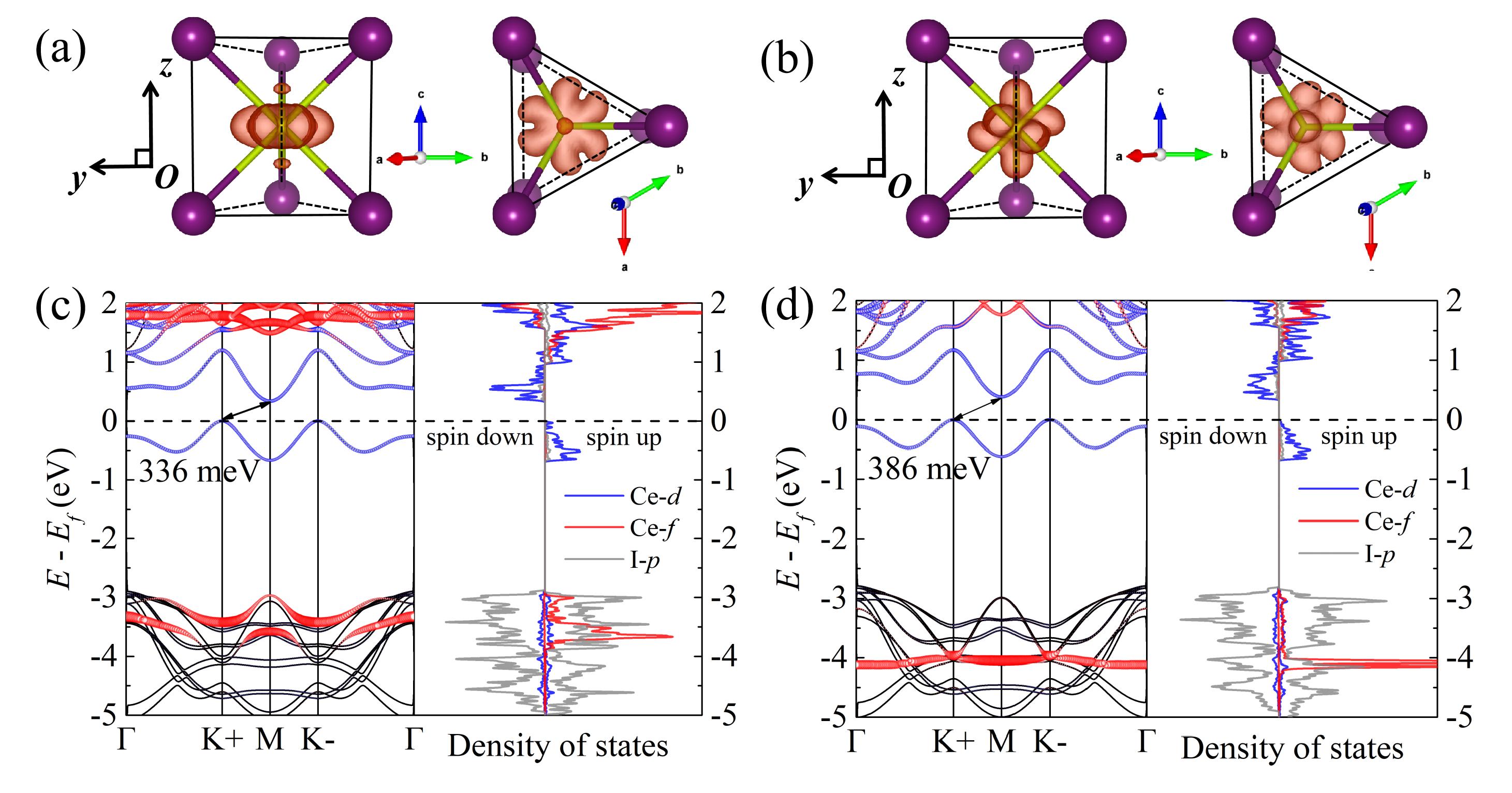
Figure 2: (Color online) The isosurfaces of spin densities for (a): S₂₀ and (b): S₀. The energy bands and density of states of (c): S₂₀ and (d): S₀. The contributions of Ce-$d$ and Ce-$f$ orbitals to the bands are represented by the blue and red bubbles, respectively.

The spin densities and electronic structures of S₂₀ and S₀ are illustrated in Fig. 2. The significant difference between the two states can be noticedby inspecting the spin densities. Meanwhile, S₀ exhibits more low-energy contributions to the bands from $4f$ orbitals than that of S₂₀. The $E-k$ dispersion of the $4f$ electron is much more weak for S₀, almost forming a flat band at $-4.1$ eV. Since there is $d-f$ hybridization on each Ce site mediated by I^- ions, the $5d$ electronic states are slightly affected by the $4f$ electronic states as well. The energy gaps of S₀ and S₂₀, which are caused by the spin splitting of the $5d$ electrons, are $386$ meV and $336$ meV, respectively. The spin densities and electronic structures of all the other states are also shown in Section F of the Supporting information.

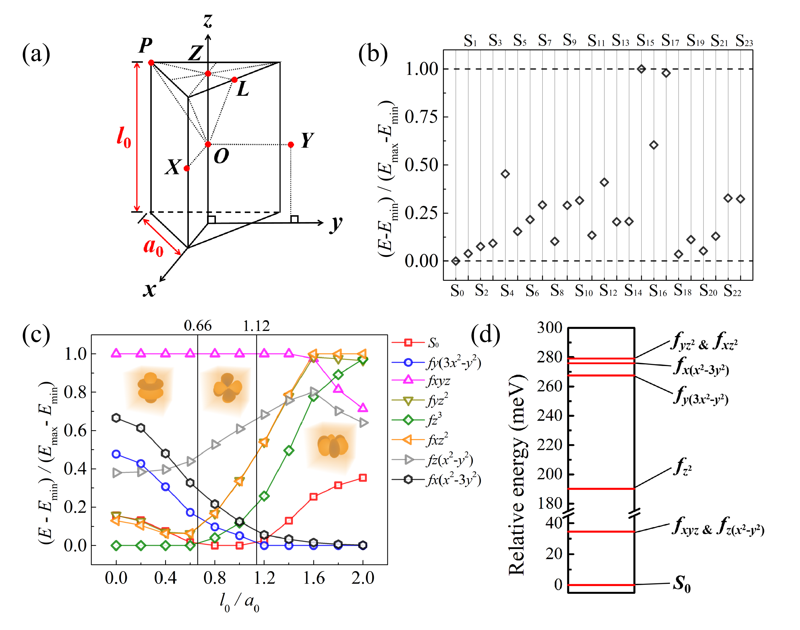
Figure 3: (Color online) (a) The RTP crystal field model in monolayer CeI₂ with the first nearest I^- ions being considered only. (b) The relative $4f$ electronic orbital energies in the RTP crystal field of the $24$ identified FM states. The lowest orbital energy is set to $0$. (c) The relative crystal field orbital energies of several $4f$ electronic orbitals with variable shape of the RTP. Here S₀ represents the single electronic orbital: $0.66f_{y(3x^{2}-y^{2})}-0.74f_{z^{3}}$. For the three ranges of $l_{0}/a_{0}$, the corresponding electronic orbital with the lowest energy is visualized. The rest of these orbitals are visualized in Section A of the Supporting information. (d) The relative DFT total energies of monolayer CeI₂ with the $4f$ electron occupying different orbitals which are discussed in (c).

V Electronic orbital energy in the RTP crystal field

In order to have a better understanding of the ground state of FM monolayer CeI₂, we calculate the electronic orbital energies of the single $4f$ electron occupying different orbitals in RTP crystal field. This so-called orbital energy is originated from pure Coulomb interactions. As shown in Fig. 3(a), the single $4f$ electron is located at $O$, with six surrounding anions located at $R_{i}$ ($x_{i}$, $y_{i}$, $z_{i}$) ($i=1,2,\cdots,6$) in the Cartesian coordinate system. The height of the RTP is denoted as $l_{0}$ and the edge length of the bottom surface is denoted as $a_{0}$. $l_{0}$ and $a_{0}$ are taken to be $4.24$ Å and $4.28$ Å, respectively, which are based on the relaxed monolayer CeI₂ by DFT calculations. The orbital energy can be expressed as

$$\left\langle E_{4f}\right\rangle=\left\langle\psi_{4f}\right|V_{\text{CF}}\left|\psi_{4f}\right\rangle,$$ (10)

where $\psi_{4f}$ is the wave function of the single $4f$ electron and $V_{\text{CF}}$ is the crystal field potential energy with a from of

$$V_{\text{CF}}=\sum_{i=1}^{6}\frac{1}{\sqrt{\left(x-x_{i}\right)^{2}+\left(y-y_{i}\right)^{2}+\left(z-z_{i}\right)^{2}}},$$ (11)

in which the constant term has been set to be unity for simplicity in the calculations. The charge densities of the six I^- ions are treated as point charges. The orbital energies of all the identified $4f^{1}$ electronic states listed in Table I are calculated. As shown in Fig. 3(b), the $4f$ electronic state for S₀ has the lowest orbital energy in the RTP crystal field. Now we can see that besides the largest value of $J^{\text{site}}$, the RTP crystal field in monolayer CeI₂ also helps to stabilize the ground state S₀ by attaching the lowest $4f$ electronic orbital energy.

We explore how the orbital energies are influenced by the shape of the RTP. The $4f$ electronic orbital of S₀ and the seven general $4f$ atomic orbitals are examined, as shown in Fig. 3(c). Keeping $a_{0}$ unchanged and $l_{0}/a_{0}$ can be taken as the unique variable. For $0<l_{0}/a_{0}<0.66$, $f_{z^{3}}$ has the lowest orbital energy. Especially when $l_{0}/a_{0}$ is equal to $0$, the crystal field is a 2D regular triangle crystal field. For $0.66<l_{0}/a_{0}<1.12$, i.e. the RTP becomes taller, the $4f$ orbital state of S₀ has the lowest orbital energy. Note that $l_{0}/a_{0}$ is equal to $0.99$ when no strain is imposed to monolayer CeI₂. For $l_{0}/a_{0}>1.12$, $f_{y(3x^{2}-y^{2})}$ has the lowest orbital energy. Now we can conclude that an appropriate shape of the RTP crystal field is indeed necessary for S₀ to maintain its lowest $4f$ electronic orbital energy. In fact, $l_{0}/a_{0}$ can only vary in a small range in monolayer CeI₂. The value of $l_{0}/a_{0}$ varies from $0.83$ (for $10\%$ tensile strain) to $1.08$ (for $5\%$ compressive strain) according to our simulations. This implies the lowest 4f electronic orbital energy for S₀ is robust in monolayer CeI₂ even if some external forces are imposed.

Since OMC is applied, the DFT total energy of the system with the $4f$ electron occupying arbitrary orbital is able to be gained as long as that $4f$ electronic state is metastable. Due to the high symmetry of the crystal field in monolayer CeI₂, the seven general $4f$ atomic orbitals are all metastable to be occupied individually. The corresponding DFT total energies are excerpted from Table I and shown in Fig. 3(d). The FM states of CeI₂ with the $4f$ electron occupying $f_{xz^{2}}$ and $f_{yz^{2}}$, respectively, are nearly degenerate and they also have equal orbital energy for the $4f$ electron referring to Fig. 3(c). However, the two states with the $4f$ electron occupying $f_{xyz}$ and $f_{z(x^{2}-y^{2})}$, respectively, are degenerate but with unequal orbital energies for the 4f electron. Since these two states also have the same value of $J^{\text{site}}$ (refer to Table I, S₁₅ and S₁₆), there should be extra factors that balance the energy difference caused by the $4f$ orbital energies. This reminds us the corresponding $5d$ electronic states should also be responsible for the total energies. A detailed discussion about this part is given in Section E of the Supporting information. In short, a complete understanding of the ground state of monolayer CeI₂ requires both $4f$ and $5d$ electronic characters although OMC is only necessary for $4f$ electrons in the DFT+U calculations.

VI The magnetic GS with strong SOC

In the more realistic situation, the electronic state of the localized 4f electron in monolayer CeI₂ is not only decided by electronic interactions, but also decided by strong SOC. Thus, the acquirement of the magnetic GS requires fully unconstrained noncollinear self-consistence calculations Worden with SOC included in the DFT+U energy functional. Here OMC is once again applied to exclude metastable states. With SOC being considered, the magnetic ground state of monolayer CeI₂ still favors FM order but the magnetic moments are with components of both $y$ and $z$ directions, as shown in Fig. 4(a). The easy axis of magnetization is coupled with the crystal field, which makes the magnetic moments point toward certain directions of the crystal structure. The ratio of the off-plane ($z$) and in-plane ($y$) components of the total magnetic moment is $0.65:1$. The net magnetic moment for each Ce is about $1.92$ $\mu$B.

Although the crystal structure of monolayer CeI₂ is only triply rotationally invariant, the magnetic GS is recommended to be six-fold degenerate by our DFT calculations. Here it is assumed that there is no difference between $z$ and $\mathtt{-}z$ directions. As displayed in Fig. 4(b), the magnetization density of magnetic GS is chiral. For two directions of magnetization marked by either two “$+$” or two “$-$”, the magnetization densities overlap completely with each other after a $\pm 2/3\pi$ rotation along $z$-axis, which are with the same chirality. For two directions of magnetization marked by “$+$” and “$-$”, respectively, the magnetization densities overlap completely with each other after a mirror-like inversion by the “$x-z$” type plane, which are with opposite chirality. As all these six magnetization densities have the equal and lowest total energy, we expect this six-fold symmetry of magnetization could be verified by the measurements of magnetic susceptibility experimentally. The SOC bands of monolayer CeI₂ is shown in Fig. 4(c). No significant and qualitative changes are detected for the electronic structure near the fermi level when compared with the situation without SOC. In spite of this, SOC is essential to reasonably describe the magnetic anisotropy in monolayer CeI₂.

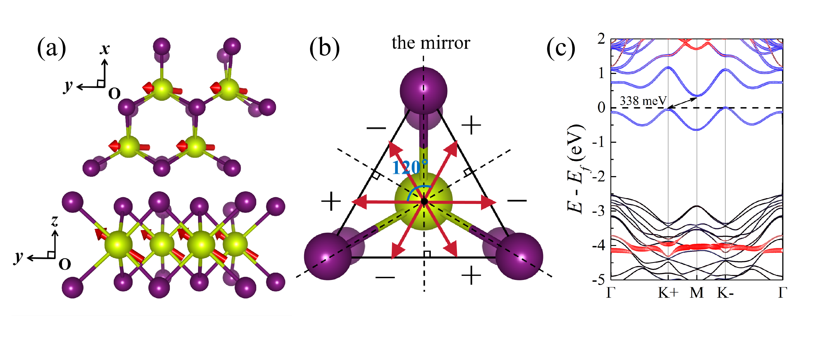
Figure 4: (Color online) (a) The FM structure of the GS of monolayer CeI₂ with SOC included. The component of x direction for the magnetic moment is strictly equal to $0$. (b) The six-fold symmetry of the magnetic GS of monolayer CeI₂ with SOC included. The red arrows only represent the in-plane component of the magnetic moments. (c) The SOC energy bands of the GS of monolayer CeI₂. The contributions of Ce-$d$ and Ce-$f$ orbitals to the bands are represented by the blue and red bubbles, respectively.

When searching for the magnetic GS of monolayer CeI₂ with SOC, a fully off-plane FM metastable state is confirmed. A comparison between this metastable state and the GS is shown in Table II. The included angle of the magnetic momentsfrom the two FM states is 57^∘ The fully off-plane FM state is $0.94$ meV per unit cell higher in total energy than the FM GS. This energy difference is obtained with the Jahn-Teller distortion of the crystal structure being considered in the simulation. If the Jahn-Teller distortion is removed, the energy difference becomes $0.72$ meV without other qualitative changes. Since the energy difference between the metastable state and the GS is small, it is expected that the monolayer CeI₂ could be easily tuned to a fully off-plane FM state with an external magnetic field. ($\sim 8.2$ T for $0.94$ meV).

Table 2: The comparison between the FM GS ($G_{\text{FM}}^{0}$) and the fully off-plane FM metastable state ($G_{\text{FM}}^{z}$) of monolayer CeI₂ with SOC included. The $2^{\text{nd}}$ column shows the magnetic moment vectors $\vec{S}$ of the two states. The $3^{\text{rd}}$ column shows the relative energies of the two states $\Delta E$ (in unit of meV). The $4^{\text{th}}$ and $5^{\text{th}}$ columns are the lattice parameters $a_{0}$ and thicknesses $l_{0}$ of monolayer CeI₂ with Jahn-Teller distortions being imposed. The $6^{\text{th }}$column shows the specific representation of the 4$f^{1}$ electronic states with $f_{y(3x^{2}-y^{2})}$, $f_{xyz}$, $f_{yz^{2}}$, $f_{z^{3}}$, $f_{xz^{2}}$, $f_{z(x^{2}-y^{2})}$, and $f_{x(x^{2}-3y^{2})}$ as bases. $\uparrow$ and $\downarrow$ denote the status of spin.

	$\vec{S}$	$\Delta E$ (meV)	$a_{0}$ (Å)	$l_{0}$ (Å)	$4f^{1}$ electronic states
$G_{\text{FM}}^{z}$	$(0,0,1)$	$0.94$	$4.28$	$4.23$	$(0.61,0,0,-0.72,0,0,0.267i)^{\uparrow}$
					$+(0,0,-0.11i,0,-0.11,0,0)^{\downarrow}$
$G_{\text{FM}}^{0}$	$(0,0.84,0.55)$	$0$	$4.29$	$4.22$	$(0.57,0,-0.15i,0.6,0,0,0.19i)^{\uparrow}$
					$+(-0.23+0.15i,0,0.14i,-0.3+0.18i,0.1,0,0)^{\downarrow}$

VII Conclusions

In this work, the ab-initio DFT+U calculations combined with OMC are performed to investigate the magnetic GS of monolayer CeI₂. The FM GS and FM metastable states are identified. It is shown that the metastable states have different magnetic properties with the magnetic GS. Thus, we recommend that something ought to be done to prevent the metastable states from producing errors when predicting the magnetic properties of such local-electron systems by DFT calculations. The $T_{\text{C}}$ of monolayer CeI₂ is simulated to be about $128$ K based on the magnetic ground state, not above room temperature as mentioned before. The calculations of on-site $d-f$ exchange parameter and $4f$ electronic orbital energy point out that the GS of monolayer CeI₂ with FM order requires the harmony of both $4f$ and $5d$ electronic states to minimize the total energy. With SOC included, the easy axis of magnetization is found to be coupled with the crystal structure. The FM GS with both in-plane and off-plane components of magnetic moments, and a fully off-plane FM metastable state of monolayer CeI₂ are confirmed to be close in total energy. Our work shows it is necessary to absorb SOC into the energy functional to allow SOC to affect the electronic state of the local electrons during the self-consistence calculations. Only in this way could the reliable magnetic GS of monolayer CeI₂ be obtained and the magnetic anisotropy be reliably described.

For other systems with local-electron magnetism, the identification of the local electronic states are also significant. However, the phenomenon of trapping into metastable states during the calculations is quite common and it causes confusions if no extra information is given. Here it is recommended to give the specific representation of the calculated local electronic state in one’s research. This action helps to enhance the repeatability and normalization of the computational studies for magnetic materials. (All the representations of the used starting points and corresponding final states in our work have been shown in Section G of the Supporting information.)

- (1) N. D. Mermin and H. Wagner, Phys. Rev. Lett. 17, 1133 (1966).
- (2) X. Jiang, Q. Liu, J. Xing, N. Liu, Y. Guo, Z. Liu, and J. Zhao, Appl. Phys. Rev. 8, 031305 (2021).
- (3) B. Huang, G. Clark, E. Navarro-Moratalla, D. R. Klein, R. Cheng, K. L. Seyler, D. Zhong, E. Schmidgall, M. A. McGuire, D. H. Cobden, W. Yao, D. Xiao, P. Jarillo-Herrero, and X. Xu, Nature 546, 270 (2017).
- (4) S. Tian, J.-F. Zhang, C. Li, T. Ying, S. Li, X. Zhang, K. Liu, and H. Lei, J. Am. Chem. Soc.141, 5326 (2019).
- (5) X. Cai, T. Song, N. P. Wilson, G. Clark, M. He, X. Zhang, T. Taniguchi, K. Watanabe, W. Yao, D. Xiao, M. A. McGuire, D. H. Cobden, and X. Xu, Nano Lett. 19, 3993 (2019).
- (6) Z. Zhang, J. Shang, C. Jiang, A. Rasmita, W. Gao, and T. Yu, Nano Lett. 19, 3138 (2019).
- (7) A. Banerjee, J. Yan, J. Knolle, C. A. Bridges, M. B. Stone, M. D. Lumsden, D. G. Mandrus, D. A. Tennant, R. Moessner, and S. E. Nagler, Science 356, 1055 (2017).
- (8) B. Zhou, Y. Wang, G. B. Osterhoudt, P. Lampen-Kelley, D. Mandrus, R. He, K. S. Burch, and E. A. Henriksen, J. Phys. Chem. Solids 128, 291 (2019).
- (9) M. Bonilla, S. Kolekar, Y. Ma, H. C. Diaz, V. Kalappattil, R. Das, T. Eggers, H. R. Gutierrez, M.-H. Phan, and M. Batzill, Nature Nanotechnol. 13, 289 (2018).
- (10) J. Li, B. Zhao, P. Chen, R. Wu, B. Li, Q. Xia, G. Guo, J. Luo, K. Zang, Z. Zhang, H. Ma, G. Sun, X. Duan, and X. Duan, Adv. Mater. 30, 1801043 (2018).
- (11) D. J. O’Hara, T. Zhu, A. H. Trout, A. S. Ahmed, Y. K. Luo, C. H. Lee, M. R. Brenner, S. Rajan, J. A. Gupta, D. W. McComb, and R. K. Kawakami, Nano Lett. 18, 3125 (2018).
- (12) C. Gong, L. Li, Z. Li, H. Ji, A. Stern, Y. Xia, T. Cao, W. Bao, C. Wang, Y. Wang, Z. Q. Qiu, R. J. Cava, S. G. Louie, J. Xia, and X. Zhang, Nature 546, 265 (2017).
- (13) X. Wang, K. Du, Y. Y. F. Liu, P. Hu, J. Zhang, Q. Zhang, M. H. S. Owen, X. Lu, C. K. Gan, P. Sengupta, C. Kloc, and Q. Xiong, 2D Mater. 3, 031009 (2016).
- (14) K. Kim, S. Y. Lim, J. Kim, J.-U. Lee, S. Lee, P. Kim, K. Park, S. Son, C.-H. Park, J.-G. Park, and H. Cheong, 2D Mater. 6, 041001 (2019).
- (15) G. Le Flem, R. Brec, G. Ouvard, A. Louisy, and P. Segransan, J. Phys. Chem. Solids 43, 455 (1982).
- (16) Z. Fei, B. Huang, P. Malinowski, W. Wang, T. Song, J. Sanchez, W. Yao, D. Xiao, X. Zhu, A. F. May, W. Wu, D. H. Cobden, J. H. Chu, and X. Xu, Nat. Mater. 17, 778 (2018).
- (17) A. F. May, D. Ovchinnikov, Q. Zheng, R. Hermann, S. Calder, B. Huang, Z. Fei, Y. Liu, X. Xu, and M. A. McGuire, ACS Nano 13, 4436 (2019).
- (18) J.-U. Lee, S. Lee, J. H. Ryoo, S. Kang, T. Y. Kim, P. Kim, C.-H. Park, J.-G. Park, and H. Cheong, Nano Lett. 16, 7433 (2016).
- (19) Y. Tian, M. J. Gray, H. Ji, R. J. Cava, and K. S. Burch, 2D Mater. 3, 025035 (2016).
- (20) Y. Deng, Y. Yu, Y. Song, J. Zhang, N. Z. Wang, Z. Sun, Y. Yi, Y. Z. Wu, S. Wu, J. Zhu, J. Wang, X. H. Chen, and Y. Zhang, Nature 563, 94 (2018).
- (21) W. Liu, Y. Xu, S. Hassan, J. Weaver, and G. van der Laan, in Handbook of Spintronics, edited by Y. Xu, D. D. Awschalom, and J. Nitta (Springer, Dordrecht, Netherlands, 2016), pp. 709–756.
- (22) G. van der Laan, Phys. Rev. Lett. 82, 640 (1999).
- (23) S. Sarikurt, Y. Kadioglu, F. Ersan, E. Vatansever, O. U. Akturk, Y. Yuksel, U. Akıncı, and E. Akturk, Phys. Chem. Chem. Phys. 20, 997 (2018).
- (24) H.-S. Kim and H.-Y. Kee, Phys. Rev. B 93, 155143 (2016).
- (25) L. J. Sandilands, Y. Tian, K. W. Plumb, Y.-J. Kim, and K. S. Burch, Phys. Rev. Lett. 114, 147201 (2015).
- (26) F. Li, K. Tu, and Z. Chen, J. Phys. Chem. C 118, 21264 (2014).
- (27) C. Ataca, H. Sahin, and S. Ciraci, J. Phys. Chem. C 116, 8983 (2012).
- (28) W. Chen, J.-m. Zhang, Y.-z. Nie, Q.-l. Xia, and G.-h. Guo, J. Magn. Magn. Mater. 508, 166878 (2020).
- (29) H.-R. Fuh, C.-R. Chang, Y.-K. Wang, R. F. L. Evans, R. W. Chantrell, and H.- T. Jeng, Sci. Rep. 6, 32625 (2016).
- (30) H. Pan, J. Phys. Chem. C 118, 13248 (2014).
- (31) M. Kan, S. Adhikari, and Q. Sun, Phys. Chem. Chem. Phys. 16, 4990 (2014).
- (32) G. T. Lin, H. L. Zhuang, X. Luo, B. J. Liu, F. C. Chen, J. Yan, Y. Sun, J. Zhou, W. J. Lu, P. Tong, Z. G. Sheng, Z. Qu, W. H. Song, X. B. Zhu, and Y. P. Sun, Phys. Rev. B 95, 245212 (2017).
- (33) M.-W. Lin, H. L. Zhuang, J. Yan, T. Z. Ward, A. A. Puretzky, C. M. Rouleau, Z. Gai, L. Liang, V. Meunier, B. G. Sumpter, P. Ganesh, P. R. C. Kent, D. B. Geohegan, D. G. Mandrus, and K. Xiao, J. Mater. Chem. C 4, 315 (2016).
- (34) H. Wang, F. Fan, S. Zhu, and H. Wu, Europhys. Lett. 114, 47001 (2016).
- (35) W.-B. Zhang, Q. Qu, P. Zhu, and C.-H. Lam, J. Mater. Chem. C 3, 12457 (2015).
- (36) J. Liu, Q. Sun, Y. Kawazoe, and P. Jena, Phys. Chem. Chem. Phys. 18, 8777 (2016).
- (37) W. Jiang, Y. Hou, S. Li, Z. Fu, and P. Zhang, Chinese Phys. B 30, 127501 (2021).
- (38) A. I. Liechtenstein, V. V. Anisimov, J. Zaanen,Phys. Rev. B 52, R5467 (1995).
- (39) S. L. Dudarev, G. A. Botton, S. Y. Savrasov, C. J. Humphreys and A. P. Sutton, Phys. Rev. B 57, 1505 (1998).
- (40) Jeremy P. Allen and Graeme W. Watson, Phys. Chem. Chem. Phys. 16, 21016-21031 (2016).
- (41) A. B. Shick, W. E. Pickett, and A. I. Liechtenstein, Journal of Electron Spectroscopy and Related Phenomena 114–116, 753-758 (2001).
- (42) A. Miskowiec, Phys. Chem. Chem. Phys. 20, 10384-10395 (2018).
- (43) B. Dorado, B. Amadon, M. Freyss, and M. Bertolus, Phys. Rev. B 79, 235125 (2009).
- (44) B. Dorado, G. Jomard, M. Freyss, and M. Bertolus, Phys. Rev. B 82, 035114 (2010).
- (45) B. Dorado, M. Freyss, B. Amadon, M. Bertolus, G. Jomardand P. Garcia, J. Phys.: Condens. Matter 25, 333201 (2013).
- (46) M. S. Christian, E. R. Johnson,and Theodore M. Besmann,J. Phys. Chem. A 125, 2791-2799 (2021).
- (47) A. Claisse, M. Klipfel, N. Lindbom, M. Freyss, and P. Olsson, Journal of Nuclear Materials 478, 119-124 (2016).
- (48) G. Jomard, B. Amadon, F. Bottin, and M. Torrent, Phys. Rev. B 78, 075125 (2008).
- (49) Y. Hou, W. Jiang, S. Li, Z. Fu, and P. Zhang, Chinese Phys. B 32, 027103 (2022).
- (50) F. Jollet, G. Jomard, and B. Amadon, Phys. Rev. B 80, 235109 (2009).
- (51) L. E Ratcliff, L. Genovese, H. Park, P. B Littlewood and Alejandro Lopez-Bezanilla, J. Phys.: Condens. Matter 34, 094003 (2022).
- (52) B. Meredig, A. Thompson, H. A. Hansen, and C. Wolverton, Phys. Rev. B 82, 195128 (2010).
- (53) H. Y. Geng, Y. Chen, Y. Kaneta, M. Kinoshita, and Q. Wu, Phys. Rev. B 82, 094106 (2010).
- (54) B. Amadon, F. Jollet, and M. Torrent, Phys. Rev. B 77, 155104 (2008).
- (55) F. Zhou and V. Ozolins, Phys. Rev. B 83, 085106 (2011).
- (56) S. Zhou, H. Ma, E. Xiao, K. Gofryk, C. Jiang, M. E. Manley, D. H. Hurley, and C. A. Marianetti, Phys. Rev. B 106, 125134 (2022).
- (57) B. Amadon, J. Phys.: Condens. Matter 24, 075604 (2012).
- (58) J. Rabone, and M. Krack, Computational Materials Science 71, 157–164 (2013).
- (59) K. Sheng, Q. Chen, H. Yuan, and Z. Wang, Phys. Rev. B 105, 075304 (2022).
- (60) Kresse G. and Furthmuller J., Phys. Rev. B 54, 11169 (1996).
- (61) Blöchl P. E., Phys. Rev. B 50, 17953 (1994).
- (62) Kresse G., Joubert D., Phys. Rev. B 59, 1758 (1999).
- (63) Blöchl P. E., Först C. J., and Schimpl J. B., Bull. Mater. Sci. 26, 33 (2003).
- (64) Perdew J. P., Burke K., and Wang Y., Phys. Rev. B 54, 16533 (1996).
- (65) P. Larson, W. R. L. Lambrecht, A. Chantis, and M. van Schilfgaarde, Phys. Rev. B 75, 045114 (2007).
- (66) A. A. Mostofi, J. R. Yates, Y. Lee, I. Souza, D. Vanderbilt, N. Marzari, Computer Physics Communications 178, 685–699 (2008).
- (67) X. He, N. Helbig, M. J. Verstraete, and E. Bousquet, Computer Physics Communications 264, 107938 (2021).
- (68) Y. Miyatake, M. Yamamoto, J. J. Kim, M. Toyonaga and O. Nagai, J. Phys. C: Solid State Phys. 19, 2539 (1986).
- (69) K. Momma and F. Izumi, J. Appl. Cryst. 41, 653-658 (2008).
- (70) V. Wang, N. Xu, J. Liu, G. Tang, and W. Geng, Computer Physics Communications 267, 108033 (2021).
- (71) B. Wang, X. Zhang, Y. Zhang, S. Yuan, Y. Guo, S. Dong and J. Wang, Mater. Horiz. 7, 1623-1630 (2020).
- (72) E. F. Worden, R. W. Solarz, and J. A. Paisner, J. Opt. Soc. Am. 68 (1978).