Optimal bounds for sensitivity sampling via augmentation
Abstract
Data subsampling is one of the most natural methods to approximate a massively large data set by a small representative proxy. In particular, sensitivity sampling received a lot of attention, which samples points proportional to an individual importance measure called sensitivity. This framework reduces in very general settings the size of data to roughly the VC dimension times the total sensitivity while providing strong guarantees on the quality of approximation. The recent work of Woodruff and Yasuda, 2023c improved substantially over the general bound for the important problem of subspace embeddings to for . Their result was subsumed by an earlier bound which was implicitly given in the work of Chen and Derezinski, (2021). We show that their result is tight when sampling according to plain sensitivities. We observe that by augmenting the sensitivities by sensitivities, we obtain better bounds improving over the aforementioned results to optimal linear sampling complexity for all . In particular, this resolves an open question of Woodruff and Yasuda, 2023c in the affirmative for and brings sensitivity subsampling into the regime that was previously only known to be possible using Lewis weights (Cohen and Peng,, 2015). As an application of our main result, we also obtain an sensitivity sampling bound for logistic regression, where is a natural complexity measure for this problem. This improves over the previous bound of Mai et al., (2021) which was based on Lewis weights subsampling.
1 Introduction
Massive data sets have become ubiquitous in recent years and standard machine learning approaches reach the limits of tractability when these large data need to be analyzed. Given a data matrix where the number of data points exceeds the number of features by a large margin, i.e., , a popular approach to address the computational limitations is to subsample the data (Munteanu,, 2023). While uniform sampling is widely used in practice, it can be associated with large loss of approximation accuracy for various machine learning models. Thus, a lot of work has been dedicated to the design of importance sampling schemes, to subsample points proportional to some sort of importance measure for the contribution of individual points, such that important points become more likely to be in the sample, while less important or redundant points are sampled with lower probability (Munteanu and Schwiegelshohn,, 2018).
General setting. The arguably most general and popular importance sampling approach is called the sensitivity framework (Feldman and Langberg,, 2011; Feldman et al.,, 2020). It aims at approximating functions applied to data that can be expressed in the following way: consider an individual non-negative loss function for each row vector of the data matrix , more precisely we set for some function . The problem we consider is approximating
| (1) |
over all in the domain , by subsampling and reweighting the individual contributions. Formally, we obtain with , and for all and define
| (2) |
to be the surrogate loss, that given an approximation parameter should be a pointwise -approximation for the original loss function. More specifically, we require that
| (3) |
The surrogate function (2) can then be used in downstream machine learning tasks, such as optimization, with very little bounded errors, and can be processed much more efficiently than the original loss. Note, that most empirical risk minimization problems or negative log-likelihood functions can be expressed as in Equation 1.
Importance subsampling. The sensitivity framework provides a way of obtaining the guarantee of Equation 3 by first computing individual sensitivities for
| (4) |
where we let when the denominator is zero. We note that computing the sensitivity is usually intractable, but it suffices to obtain close approximations, which can be done efficiently for many important problems.
Then, subsampling with probabilities proportional to and reweighting the individual contributions by , preserves the objective function in expectation and when , we obtain by a concentration result that the -approximation defined in Equation 3 holds with constant probability. Here, is the VC dimension of a set system associated with the functions , and denotes their total sensitivity.
Subspace embeddings for . In this paper, we focus on applying the above framework to the more specific, yet very versatile problem of constructing a so-called subspace embedding via subsampling. Given a data matrix with row-vectors , and a norm parameter , our goal is to calculate probabilities , and weights for each , such that a small random subsample according to this distribution satisfies
| (5) |
with probability at least .
We remark at this point that since the norms are absolutely homogeneous, previous work usually includes the weights by folding them into the data, i.e., becomes . This usually allows to simplify large parts of the technical analysis by reducing to the unweighted case. We explicitly do not use this trick for reasons to be discussed later.
With the definition of our main problem in place, we next define the sensitivity measure associated with this loss function and note that they are also called leverage scores in our scope.
Definition 1.1 (-sensitivities/-leverage scores).
Let , and . We define the -th -sensitivity or -leverage score of to be
and the total sensitivity as .
It can be shown in some settings, that the total sensitivity is a lower bound on the required number of samples (cf. Tolochinsky et al.,, 2022), and is a natural lower bound for our problem because this number of samples is required to even preserve the rank of under subsampling. It is also known that for all (cf. Woodruff and Yasuda, 2023c, ). Thus, a natural question to ask is whether it is possible to obtain the guarantee of Equation 5 within roughly samples.
A plain application of the sensitivity framework requires samples, and a lower bound of was given by Li et al., (2021) in a broader setting against any data structure that answers subspace queries. The sensitivity sampling upper bound thus seems off by a factor , and the recent work of Woodruff and Yasuda, 2023c has made significant progress by showing that one can do better for all . They obtained near optimal bounds when becomes close to . In this particular case, a bound was known before to be possible by leverage score sampling (Mahoney,, 2011). However, near the boundary (and for ) the bounds of Woodruff and Yasuda, 2023c are again off by a factor . In the case , the previous work of Chen and Derezinski, (2021) gave better results that were achieved implicitly by relating leverage scores to Lewis weights. Again, these bounds become worse when and are off by a factor for . See below for a more detailed comparison between these works, and our work.
This brings us to the main open question in this line of research, which is also the central question studied in our paper:
Question 1.2.
Is it possible to achieve a sampling complexity of for constructing an subspace embedding, see Equation 5, via sensitivity sampling?
1.1 Our contribution
Our first contribution is an lower bound against pure leverage score sampling, i.e., when the sampling probabilities are proportional to .
Theorem 1.3 (Informal restatement of Theorem B.1).
There exists a matrix , for sufficiently large , such that if we sample each row with probability for some , then with high probability, the subspace embedding guarantee (see Equation 5) does not hold unless .
The proof in the appendix is conducted by constructing a matrix with two parts. Subsampling at least rows of each part is necessary to even preserve the rank. However, the total sensitivity of one part is significantly larger than the total sensitivity of the other part, roughly by a factor of . This implies that leverage score sampling requires oversampling by that factor to collect the required rows from both parts, which yields the lower bound.
In particular, Theorem 1.3 proves that the upper bounds implied by Chen and Derezinski, (2021) for pure leverage score sampling are optimal in the worst case, settling the complexity of pure sampling up to polylogarithmic factors. It also proves that we necessarily need to change the sampling probabilities to get below the lower bound towards optimal linear dependence. We note that augmentation by uniform sampling does not help, since the size of the high sensitivity part can be increased to give the same imbalance between the number of rows of the two parts as between their sampling probabilities in pure sampling.
Our main result is the following sensitivity sampling bound that is achieved by augmenting with sensitivities, a new technique that we call “ augmentation”. The theorem answers 1.2 in the affirmative for all , improving over Chen and Derezinski, (2021); Woodruff and Yasuda, 2023c , and settling the complexity of subspace embeddings via sensitivity sampling in this regime. We leave the case as an open question, where our work resembles the same bounds as Woodruff and Yasuda, 2023c .
Our theorem is generalized to also hold for the variant of the ReLU function where . For this loss function, we also require a data dependent mildness parameter to be bounded.
Definition 1.4 (-complexity, Munteanu et al.,, 2018, 2022, slightly modified).
Given a data set we define the parameter as
where , and are the vectors comprising only the positive resp. negative entries of and all others set to .111To see that the suprema are equal, one can flip signs: for any the suprema range over, we have that .
For the main problem where , we can remove this parameter or equivalently set .
Theorem 1.5 (Informal restatement of Theorem G.1).
Let . Let , . Consider for , where we set , or , in which case , see Definition 1.4. Set Let be a sample of size
where the probability for any satisfies
and the corresponding weight is set to . Then with probability at least it holds for all simultaneously that
As an application, we extend our main result to hold for the logistic loss function as well. This improves over the previous bound of Mai et al., (2021) which was based on Lewis weights subsampling.
Theorem 1.6 (Informal restatement of Theorem H.4).
Let . Let with , see Definition 1.4. Consider with the logistic loss . Further assume that we sample with probabilities for , where the number of samples is
Then with probability at least it holds for all simultaneously that
1.2 Comparison to related work
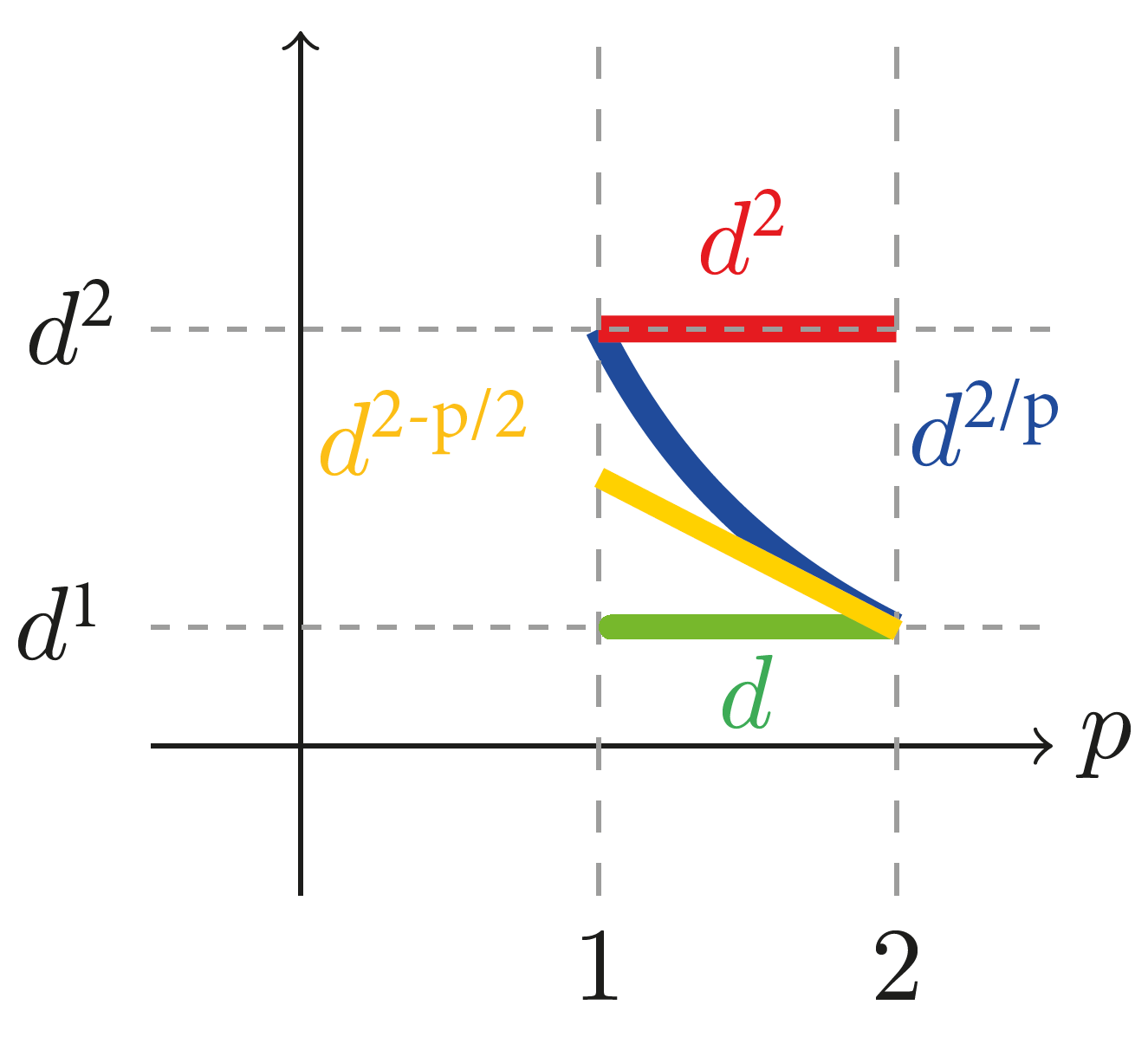
For subspace embeddings, the total sensitivity is bounded by , for , and by for , (cf. Woodruff and Yasuda, 2023c, ). It is known that using so-called Lewis weights, we can subsample a nearly optimal amount respectively of rows to obtain the subspace embedding guarantee of Equation 5, (see Cohen and Peng,, 2015; Woodruff and Yasuda, 2023b, ). Recent work of Jambulapati et al., (2023) recovers matching bounds via a novel sampling distribution, and for a broad array of semi-norms. On the other hand, using sensitivity sampling in a plain application of the sensitivity framework requires , which is off by a factor in the worst case for any value of .
Recently improved sensitivity sampling bounds of Woodruff and Yasuda, 2023c are for and for . These bounds are much better than the standard bounds when is close to the case , but they deteriorate towards and , where the gap is again a factor of . For their worst case bounds are even worse than the plain sensitivity framework. We note that Woodruff and Yasuda, 2023c gave an improved bound for this regime as well, albeit not with a direct sensitivity sampling approach. Instead, they gave an algorithm that recursively ’flattens and samples’ heavy rows with respect to their sensitivities for and .
Although improving over the standard bounds for as well, the main improvement of Woodruff and Yasuda, 2023c lies in the case . This is because prior to their results, Chen and Derezinski, (2021) implicitly showed a bound of by relating sensitivities to Lewis weights up to an additional factor of . Oversampling the sensitivity scores by this amount guarantees that the increased scores exceed the Lewis weights, which in turn implies a sampling complexity of to be sufficient. We show in Theorem 1.3 that their bound is tight up to polylogarithmic factors in the worst case, when , if we sample according to pure leverage scores.
This leads us to our main result, Theorem 1.5, which samples for any value of a number of many samples according to a mixture of , and sensitivities with a uniform distribution . This technique relies only on sensitivity sampling and in the worst case, the number of samples amounts to for all . We note that this matches up to polylogarithmic factors the optimal complexities obtained by Lewis weights, and by other novel sampling probabilities (Cohen and Peng,, 2015; Woodruff and Yasuda, 2023b, ; Jambulapati et al.,, 2023). See Figure 1 for a visual comparison of our bounds with previous sensitivity sampling bounds.
Sample complexity bounds for sensitivity sampling
In particular, note that our bounds improve the respectively dimension dependence of previous bounds for to linear. This allows an application to logistic regression (Theorem 1.6), obtaining up to polylogarithmic factors a sampling bound of . Previously, the linear dependence on was only known to be possible using Lewis weights (Mai et al.,, 2021; Woodruff and Yasuda, 2023b, ). In fact our result even improves over their bound by a factor of , a complexity parameter introduced by Munteanu et al., (2018, 2022) for compressing data in the scope of logistic regression and other asymmetric functions. We note that linear and (near-)linear dependence was recently achieved in the sketching regime, though at the cost of constant approximation factors Munteanu et al., (2023). We remark that our polylogarithmic dependencies hidden in the notation are only and do not depend on , which is also a minor improvement compared to almost all mentioned previous works.
Our paper assumes that we have access to sensitivity scores, without giving details on how to compute or approximate them. We refer to (Dasgupta et al.,, 2009; Woodruff and Zhang,, 2013; Clarkson et al.,, 2016; Munteanu et al.,, 2022) for classic techniques such as ellipsoidal rounding and well-conditioned bases, as well as to recent advances in constructing improved well-conditioned bases (Wang and Woodruff,, 2022), novel spanning sets (Woodruff and Yasuda, 2023a, ; Bhaskara et al.,, 2023), or direct sensitivity approximations (Padmanabhan et al.,, 2023). We also refer to (Mahabadi et al.,, 2020; Munteanu and Omlor,, 2024) for sensitivity sampling in data streams.
One might argue that the sensitivity sampling approach is not very interesting for , since Lewis weights, among others, already obtain optimal bounds in this regime. However, leverage scores are usually simpler to calculate or to approximate. For instance Cohen and Peng, (2015); Mai et al., (2021) calculate an approximation to Lewis weights by recursively reweighting the data and computing leverage scores times over and over again. While the factor overhead seems minor from a theoretical perspective, this slows down computations by a non-negligible amount. We refer to (Mai et al.,, 2021; Munteanu et al.,, 2022) for details, where computational issues have been discussed and demonstrated in experiments.
The experiments in (Mai et al.,, 2021; Munteanu et al.,, 2022) also suggest that sensitivity sampling works much better than indicated by upper bounds, sometimes even better than Lewis weights. It is thus very important to find a theoretical explanation for the success of sensitivity sampling and to find out whether they also achieve the optimal complexity or if there are lower bounds preventing them from achieving optimality. This is the motivation behind our work.
We would like to mention that very similar findings have been observed in the center-based clustering regime, where group sampling was known to produce subsamples of optimal size (Cohen-Addad et al.,, 2021, 2022; Huang et al.,, 2022). But group sampling was often outperformed by the conceptually and computationally simpler sensitivity sampling approach on practical and on hard instances (Schwiegelshohn and Sheikh-Omar,, 2022). Independently of our work, this was explained in Bansal et al., (2024) by proving that sensitivity sampling also achieves optimal subsample size for -means and -median clustering.
Further, sensitivity sampling has already been studied for a plethora of problems such as regression (Dasgupta et al.,, 2009), -estimators (Clarkson and Woodruff, 2015b, ; Clarkson and Woodruff, 2015a, ), near-convex functions (Tukan et al.,, 2020), logistic regression (Munteanu et al.,, 2018), other generalized linear models such as probit regression (Munteanu et al.,, 2022), Poisson and graphical models (Molina et al.,, 2018), IRT models in educational sciences and psychometrics (Frick et al.,, 2024). Also, some seemingly more distant works have strong connections to sensitivity sampling, such as graph sparsification using effective resistances (Spielman and Srivastava,, 2011). Our new optimal bounds for all cover the most common regime encountered in all of these works and will thus be useful in obtaining improved bounds for a broad array of applications as well.
2 New sensitivity subsampling bounds
Our analysis uses several results of Woodruff and Yasuda, 2023c , and our main argumentation follows their general outline. Since our analysis is in wide parts a strict generalization, the worst possible outcome of our investigations would simply resemble their exact same bounds. As we have indicated previously, this is actually the case for in which our techniques do not improve over their bounds. The corresponding part of the analysis is therefore not contained in our paper and we focus on the regime in the remainder.
One main technical argument in this regime is that by monotonicity of maximal sensitivities, the largest leverage score upper bounds the largest leverage score. To leverage this fact, previous analyses relied on an auxiliary subspace embedding for obtaining a constant factor subspace embedding that required overhead.
In our analysis, we bypass this problem by adding the leverage scores to the sensitivity upper bound that defines our sampling probabilities. Intuitively, this allows us to obtain the subspace embedding guarantee for and simultaneously: the subspace embedding is known to hold already for small sample size . Taking it from here, it enables the subspace embedding to work with little more samples. Fortunately, this overhead is negligible compared to the small sample already taken, and also smaller compared to the previous bounds to obtain the subspace embedding directly. Note that also reversely, the data matrix might have much smaller total sensitivity than . In this case, augmenting the sample to at least the rank preserving lower bound can be accomplished with the least number of additional samples by sensitivity sampling.
The main reason why the previous analyses do not admit a simultaneous and subspace embedding, is that they tend to fold the weights into the data (or into the sampling matrix), rather than keeping the weights separately. This is a nice trick which simplifies wide parts of previous analyses by reducing the weighted case to the unweighted case. However, it prevents from our goals as we show in the following simple, yet instructive example for simultaneous and embedding, which requires to store the weights separately:
Take to be the matrix consisting of copies of the row vector . Note that for we have that and . We wish to construct a subspace embedding, preserving both norms up to a factor of two. To this end, assume that we have a reduced and reweighted matrix with . Then we also have that . Now, we also require that . Combining both inequalities implies that which is equivalent to . We conclude that any subspace embedding without auxiliary weights that preserves both, the , and the norm up to a factor of requires at least rows.
In stark contrast to this impossibility result, using probabilities , standard sensitivity sampling allows us to take samples and reweight them by such that , and hold simultaneously.
To leverage this fact and improve the sampling complexity to linear, we need to open up and generalize large parts of the work of Woodruff and Yasuda, 2023c to deal with weighted norms, which we define as follows:
Definition 2.1.
Given a vector , and weights , we let
For the norm, we also let
and
2.1 Outline of the analysis
The full formal details can be found in the appendix. Here we provide an outline for the proofs of our main results. We note that some definitions or notation might slightly differ from the appendix for the sake of a clean and concise presentation. The proof consists of several main steps for which we give high level descriptions:
2.1.1 Bounding by a Gaussian process
The first step is to bound the approximation error by a Gaussian process. Note that the subspace embedding guarantee of Equation 3 will be achieved when
where , and is a sampling matrix with exactly one non-zero entry in each row such that consists of rows out of from the data matrix . By homogeneity of the loss functions, we can restrict the analysis to the case that , and our goal is to bound the above term by .
To this end, we bound higher moments of the expected error using a standard symmetrization and Gaussianization argument by
where the expectation is taken over the random subsample, represented by , and on the right hand side additionally over i.i.d. standard Gaussians .
The sum on the right hand side is a Gaussian process that induces a pseudo metric, such that for all , we have
acting in the reduced and reweighted space.
For bounding the Gaussian process, we use a slightly adapted moment bound of Woodruff and Yasuda, 2023c
which follows from a tail bound due to Sudakov, which is sometimes attributed to Dudley. See (Dudley,, 2016; Ledoux and Talagrand,, 1991) for bibliographical discussion and references.
Here, is a sufficiently large absolute constant, is an upper bound on the entropy of the Gaussian process, and is an upper bound on the diameter of the set according to the pseudo-metric, i.e.,
Note, that we can accomplish our goal by using the moment bound for an appropriately large choice of and applying Markov’s inequality. Our remaining task thus reduces to bounding the diameter, and the entropy, and to quantify the required value of , which will also determine a sufficient subsample size.
2.1.2 Bounding the diameter
We bound the diameter by relating it to the approximation error and to the largest possible coordinate in the reduced and reweighted norm vector among all vectors that satisfy . More specifically, let
Note that is similar to the largest leverage score. Also define
Then we prove that the diameter with respect to the pseudo metric is bounded by
We remark here, that this requires special care when treating the -ReLU function so not to loose additional factors unnecessarily. But in the final step, it can simply be upper bounded by the proper norm function since for all . Thus, the same diameter bound applies to both functions without additional dependence.
2.1.3 Bounds on covering numbers
Before we can proceed with bounding the entropy of the Gaussian process, we first need to bound the smallest number of (weighted) balls of certain radius that are required to cover balls, for various values of .
To this end, we define balls according to the weighted norms. Given a Matrix , a weight vector and , we set
For any and , let the covering number denotes the minimum cardinality of a set of balls of radius required to cover the unit ball. That is, is chosen such that for any there exists with . This enables chaining arguments to construct a sequence of -nets at different scales, which can be smaller than using one single -net, i.e., one fixed scale for the entire space. See Nelson, (2016) for a survey on chaining techniques and applications.
To bound the covering numbers, we aim at applying a so-called Dual-Sudakov-minoration result (see Bourgain et al.,, 1989). Let be a norm, and let denote the Euclidean unit ball in dimensions. Then,
where denotes the Lévy mean
It is well known that the denominator is , therefore the previous bound reduces to
A very important step in the proof is thus the following bound, which also required to be reproved to account for the weighted norm for .
Consider an orthonormal matrix and . Let be the largest weighted leverage score. Then we have that
Here is also where the leverage scores play a role in our bounds, and will later be used together with the leverage scores in order to balance the diameter bound with the entropy bound.
This bound allows us to control the covering numbers for various norms, including the norm for the respective weighted balls. In particular, we obtain bounds on the number of weighted balls required to cover weighted balls, by first covering using balls and then covering each ball again with balls. Applying a chaining technique using a telescoping sum over varying scales, yields a bound of roughly
| (6) |
2.1.4 Bounding the entropy
For bounding the entropy, we need to control the following quantity
To this end, we first derive the following final covering bounds: one for small with a logarithmic dependence on and a different bound for larger with a squared dependence on but lower dependence on .
The first item follows by relating to the unweighted case, where a simple net construction suffices, i.e.,
In fact, this is the only place in our proof where the weighted case can simply be reduced to the unweighted case. The second bound follows by applying the previous Equation 6.
We split the entropy integral at an appropriate point into
where the latter can be cut off at our previous diameter bound because when the integral exceeds the diameter, it becomes .
The two parts of the integral can now be bounded using the covering bounds respectively from above. That is, for small radii less than we use the first bound and for radii larger than , we use the the second bound.
Choosing the right value for so as to keep both terms appropriately small, we obtain the following entropy bound:
Note, in particular the dependence on the weighted largest leverage score which will be crucial to balance the diameter with the entropy bound in the main proof.
2.1.5 Outline of the main proof
We have now worked out all pieces that we need in order to prove our main result given in Theorem 1.5. Again, we refer to the appendix for the full technical details. Here, we present a sketch of the final proof:
Let us begin with the sample size . This is handled in a standard way by defining an indicator random variable that attains if row is in the sample and otherwise it attains . The expected size equals
Since , , and , we can thus bound the expected size by
An application of Chernoff’s bounds yields in particular that holds with probability at least .
Next, note that by our choice of it holds that , and each sample is taken with probability . This is sufficient to achieve the norm subspace embedding up to a factor with probability at least (Mahoney,, 2011).
It allows us to relate to the largest weighted leverage score of the original matrix, rather than the subsample, i.e.,
We assume without loss of generality that and thus noting that , we have that and thus . A very similar argument yields . Consequently, we have that
Plugging this into our diameter bound, we obtain
where for a suitable constant.
Plugging this into the entropy integral bound, we obtain
Finally, we found bounds for , and which are suitably balanced and allow us to apply the moment bound of Woodruff and Yasuda, 2023c , which yields
for suitably large absolute constants .
Using this higher moment bound in an application of Markov’s inequality, we get that holds with probability at least , since
This concludes the proof by taking a union bound over the three probabilistic events, and rescaling and respectively.
3 Application to logistic regression
Here we provide an outline and some high level intuition behind the proof of our second result given in Theorem 1.6.
The logistic loss function is given by
so in our previous notation we have to deal with individual loss functions .
Unfortunately, does not fully satisfy the assumptions of our main theorem. Therefore, we cannot apply Theorem 1.5 directly. Instead, we observe that can be rewritten in terms of the coordinate-wise ReLU function and the remainder.
We thus split into two parts as follows:
Using this split, we show that taking a sample with probabilities where preserves the logistic loss function for all up to a relative error of at most . Note, that we oversample only by a linear factor .
Indeed, this allows the -ReLU function , with to be handled by a direct application of our main result, which yields
The remaining part is a bounded function, and can be handled by the uniform part of our sample. We note that this can be proven by a simple additive concentration bound, and charging the additive error by the optimal cost.
We take a slight detour using the standard sensitivity framework, which allows us to draw from existing previous work and saves a lot of technicalities. To this end, we restrict the function to the negative domain to obtain with .
Now, observe that can be rewritten as
where
and
Next, we observe that since , and , we have that each sensitivity for both of the two functions is bounded by , and the total sensitivity is .
Using the strict monotonicity of both functions, we can relate the VC dimension of a set system associated with the two functions to the VC dimension of affine hyperplane classifiers. Using a thresholding and rounding trick, this yields a final VC dimension bound of . These arguments are standard from recent literature, see Munteanu et al., (2018, 2022) for details.
Putting the VC dimension and sensitivity bounds into the standard sensitivity framework and defining the approximate functions
and similarly
yields for both separately that
each with probability at least .
Now, by a union bound, and using the triangle inequality we can put all three approximations together, which yields
with probability at least . We conclude the proof by rescaling , and .
As a final remark, previous work aimed at approximating the coordinate-wise ReLU function by bounding the error additively to within an fraction of the norm and then using a rescaled to relate the norm back to the ReLU function.
Since the dependence on is typically quadratic, this approach is prone to a factor in the final sample size. Our direct approximation of the ReLU function handled via Theorem 1.5 requires oversampling by only , which results in a linear dependence for logistic regression as well.
4 Conclusion and open directions
In this paper, we resolve the sample complexity of subspace embedding via sensitivity sampling for all .
Specifically, our work establishes new lower bounds against pure leverage score sampling, showing that upper bounds implied by previous work of Chen and Derezinski, (2021) are tight in the worst case up to polylogarithmic factors.
By generalizing the approach of Woodruff and Yasuda, 2023c to deal with weighted norms and augmenting sampling probabilities with leverage scores, our work strengthens previous upper bounds of Chen and Derezinski, (2021); Woodruff and Yasuda, 2023c for all to linear sample complexity, matching known lower bounds by Li et al., (2021) in the worst case.
In particular, this resolves an open question of Woodruff and Yasuda, 2023c in the affirmative for and brings the conceptually and computationally simple sensitivity subsampling approach into the regime that was previously only known to be possible using Lewis weights (Cohen and Peng,, 2015), or other alternatives Jambulapati et al., (2023).
As an application of our results, we also obtain the first fully linear bound for approximating logistic regression, obtained via a special treatment of the -generalization of the ReLU function, and improving over a previous bound (Mai et al.,, 2021) as well as over bounds with . Our -generalization of the ReLU function suggests similar improvements for -generalized probit regression (Munteanu et al.,, 2022), which we leave as an open problem.
We note that in the case of , our generalization does not yield an improvement over the previous bounds of Woodruff and Yasuda, 2023c . Therefore, obtaining bounds or any improvement towards that goal remains an important open problem for future research. Further, we hope that our methods will help to improve sensitivity sampling bounds for other, more general loss functions, and distance based loss functions beyond norms.
Acknowledgements
The authors would like to thank the anonymous reviewers of ICML 2024 for very valuable comments and discussion. This work was supported by the German Research Foundation (DFG), grant MU 4662/2-1 (535889065), and by the Federal Ministry of Education and Research of Germany (BMBF) and the state of North Rhine-Westphalia (MKW.NRW) as part of the Lamarr-Institute for Machine Learning and Artificial Intelligence, Dortmund, Germany. Alexander Munteanu was additionally supported by the TU Dortmund - Center for Data Science and Simulation (DoDaS).
References
- Bansal et al., (2024) Bansal, N., Cohen-Addad, V., Prabhu, M., Saulpic, D., and Schwiegelshohn, C. (2024). Sensitivity sampling for -means: Worst case and stability optimal coreset bounds. CoRR, abs/2405.01339.
- Bhaskara et al., (2023) Bhaskara, A., Mahabadi, S., and Vakilian, A. (2023). Tight bounds for volumetric spanners and applications. In Advances in Neural Information Processing Systems 36 (NeurIPS).
- Bourgain et al., (1989) Bourgain, J., Lindenstrauss, J., and Milman, V. (1989). Approximation of zonoids by zonotopes. Acta Math, 162(1-2):73–141.
- Chen and Derezinski, (2021) Chen, X. and Derezinski, M. (2021). Query complexity of least absolute deviation regression via robust uniform convergence. In Conference on Learning Theory (COLT), pages 1144–1179.
- Clarkson et al., (2016) Clarkson, K. L., Drineas, P., Magdon-Ismail, M., Mahoney, M. W., Meng, X., and Woodruff, D. P. (2016). The fast Cauchy transform and faster robust linear regression. SIAM Journal on Computing, 45(3):763–810.
- (6) Clarkson, K. L. and Woodruff, D. P. (2015a). Input sparsity and hardness for robust subspace approximation. In Guruswami, V., editor, IEEE 56th Annual Symposium on Foundations of Computer Science (FOCS), pages 310–329.
- (7) Clarkson, K. L. and Woodruff, D. P. (2015b). Sketching for M-estimators: A unified approach to robust regression. In Proceedings of the 26th Annual ACM-SIAM Symposium on Discrete Algorithms (SODA), pages 921–939.
- Cohen and Peng, (2015) Cohen, M. B. and Peng, R. (2015). row sampling by Lewis weights. In Proceedings of the Forty-Seventh Annual ACM on Symposium on Theory of Computing (STOC), pages 183–192.
- Cohen-Addad et al., (2022) Cohen-Addad, V., Larsen, K. G., Saulpic, D., Schwiegelshohn, C., and Sheikh-Omar, O. A. (2022). Improved coresets for Euclidean k-means. In Advances in Neural Information Processing Systems 35 (NeurIPS).
- Cohen-Addad et al., (2021) Cohen-Addad, V., Saulpic, D., and Schwiegelshohn, C. (2021). A new coreset framework for clustering. In 53rd Annual ACM SIGACT Symposium on Theory of Computing (STOC), pages 169–182.
- Dasgupta et al., (2009) Dasgupta, A., Drineas, P., Harb, B., Kumar, R., and Mahoney, M. W. (2009). Sampling algorithms and coresets for regression. SIAM J. Comput., 38(5):2060–2078.
- Dudley, (2016) Dudley, R. M. (2016). V.N. Sudakov’s work on expected suprema of Gaussian processes. In Houdré, C., Mason, D. M., Reynaud-Bouret, P., and Rosiński, J., editors, High Dimensional Probability VII, pages 37–43. Springer International Publishing.
- Feldman and Langberg, (2011) Feldman, D. and Langberg, M. (2011). A unified framework for approximating and clustering data. In Proceedings of the 43rd ACM Symposium on Theory of Computing (STOC), pages 569–578.
- Feldman et al., (2020) Feldman, D., Schmidt, M., and Sohler, C. (2020). Turning Big Data into tiny data: Constant-size coresets for k-means, PCA, and projective clustering. SIAM J. Comput., 49(3):601–657.
- Frick et al., (2024) Frick, S., Krivosija, A., and Munteanu, A. (2024). Scalable learning of item response theory models. In International Conference on Artificial Intelligence and Statistics (AISTATS), pages 1234–1242.
- Huang et al., (2022) Huang, L., Li, J., and Wu, X. (2022). Towards optimal coreset construction for (k,z)-clustering: Breaking the quadratic dependency on k. CoRR, abs/2211.11923.
- Jambulapati et al., (2023) Jambulapati, A., Lee, J. R., Liu, Y. P., and Sidford, A. (2023). Sparsifying sums of norms. In 64th IEEE Annual Symposium on Foundations of Computer Science (FOCS), pages 1953–1962.
- Langberg and Schulman, (2010) Langberg, M. and Schulman, L. J. (2010). Universal -approximators for integrals. In Proceedings of the Twenty-First Annual ACM-SIAM Symposium on Discrete Algorithms (SODA), pages 598–607.
- Ledoux and Talagrand, (1991) Ledoux, M. and Talagrand, M. (1991). Probability in Banach Spaces: isoperimetry and processes, volume 23. Springer Science & Business Media.
- Li et al., (2021) Li, Y., Wang, R., and Woodruff, D. P. (2021). Tight bounds for the subspace sketch problem with applications. SIAM J. Comput., 50(4):1287–1335.
- Mahabadi et al., (2020) Mahabadi, S., Razenshteyn, I. P., Woodruff, D. P., and Zhou, S. (2020). Non-adaptive adaptive sampling on turnstile streams. In Proccedings of the 52nd Annual ACM SIGACT Symposium on Theory of Computing (STOC), pages 1251–1264.
- Mahoney, (2011) Mahoney, M. W. (2011). Randomized algorithms for matrices and data. Found. Trends Mach. Learn., 3(2):123–224.
- Mai et al., (2021) Mai, T., Musco, C., and Rao, A. (2021). Coresets for classification - simplified and strengthened. In Advances in Neural Information Processing Systems 34 (NeurIPS), pages 11643–11654.
- Molina et al., (2018) Molina, A., Munteanu, A., and Kersting, K. (2018). Core dependency networks. In Proceedings of the Thirty-Second AAAI Conference on Artificial Intelligence (AAAI), pages 3820–3827.
- Munteanu, (2023) Munteanu, A. (2023). Coresets and sketches for regression problems on data streams and distributed data. In Machine Learning under Resource Constraints, Volume 1 - Fundamentals, pages 85–98. De Gruyter, Berlin, Boston.
- Munteanu and Omlor, (2024) Munteanu, A. and Omlor, S. (2024). Turnstile leverage score sampling with applications. In Proceedings of the 41st International Conference on Machine Learning (ICML).
- Munteanu et al., (2022) Munteanu, A., Omlor, S., and Peters, C. (2022). -Generalized probit regression and scalable maximum likelihood estimation via sketching and coresets. In Proceedings of the 25th International Conference on Artificial Intelligence and Statistics (AISTATS), pages 2073–2100.
- Munteanu et al., (2021) Munteanu, A., Omlor, S., and Woodruff, D. P. (2021). Oblivious sketching for logistic regression. In Proceedings of the 38th International Conference on Machine Learning (ICML), pages 7861–7871.
- Munteanu et al., (2023) Munteanu, A., Omlor, S., and Woodruff, D. P. (2023). Almost linear constant-factor sketching for and logistic regression. In The Eleventh International Conference on Learning Representations (ICLR).
- Munteanu and Schwiegelshohn, (2018) Munteanu, A. and Schwiegelshohn, C. (2018). Coresets-methods and history: A theoreticians design pattern for approximation and streaming algorithms. Künstliche Intell., 32(1):37–53.
- Munteanu et al., (2018) Munteanu, A., Schwiegelshohn, C., Sohler, C., and Woodruff, D. P. (2018). On coresets for logistic regression. In Advances in Neural Information Processing Systems 31 (NeurIPS), pages 6562–6571.
- Nelson, (2016) Nelson, J. (2016). Chaining introduction with some computer science applications. Bull. EATCS, 120.
- Padmanabhan et al., (2023) Padmanabhan, S., Woodruff, D. P., and Zhang, R. (2023). Computing approximate sensitivities. In Advances in Neural Information Processing Systems 36 (NeurIPS).
- Schwiegelshohn and Sheikh-Omar, (2022) Schwiegelshohn, C. and Sheikh-Omar, O. A. (2022). An empirical evaluation of k-means coresets. In 30th Annual European Symposium on Algorithms (ESA), pages 84:1–84:17.
- Spielman and Srivastava, (2011) Spielman, D. A. and Srivastava, N. (2011). Graph sparsification by effective resistances. SIAM J. Comput., 40(6):1913–1926.
- Tolochinsky et al., (2022) Tolochinsky, E., Jubran, I., and Feldman, D. (2022). Generic coreset for scalable learning of monotonic kernels: Logistic regression, sigmoid and more. In International Conference on Machine Learning (ICML), pages 21520–21547.
- Tukan et al., (2020) Tukan, M., Maalouf, A., and Feldman, D. (2020). Coresets for near-convex functions. In Advances in Neural Information Processing Systems 33 (NeurIPS).
- Wang and Woodruff, (2022) Wang, R. and Woodruff, D. P. (2022). Tight bounds for oblivious subspace embeddings. ACM Trans. Algorithms, 18(1):8:1–8:32.
- (39) Woodruff, D. P. and Yasuda, T. (2023a). New subset selection algorithms for low rank approximation: Offline and online. In Proceedings of the 55th Annual ACM Symposium on Theory of Computing (STOC), pages 1802–1813.
- (40) Woodruff, D. P. and Yasuda, T. (2023b). Online Lewis weight sampling. In Proceedings of the 2023 ACM-SIAM Symposium on Discrete Algorithms (SODA), pages 4622–4666.
- (41) Woodruff, D. P. and Yasuda, T. (2023c). Sharper bounds for sensitivity sampling. In International Conference on Machine Learning (ICML), pages 37238–37272.
- Woodruff and Zhang, (2013) Woodruff, D. P. and Zhang, Q. (2013). Subspace embeddings and -regression using exponential random variables. In The 26th Annual Conference on Learning Theory (COLT), pages 546–567.
Appendix A Setting
We are given some dataset consisting of points for where . We set to be the matrix with rows . Further we are given a possibly weighted function for some function that measures the contribution of each point. We drop the subscript if the weights are uniformly for all
Specifically, we consider in this paper and for . We will also extend the latter case for to logistic regression .
Our goal is to show that when sampling with probability proportional to a mixture of the -leverage scores, the -leverage scores and , then with a sample of elements we can guarantee with failure probability at most that it holds that
| (7) |
where is a sampling matrix with exactly one non-zero entry in each row such that extracts rows out of from the data matrix , see Definition C.6.
We first prove a lower bound against pure leverage score sampling. The remainder is dedicated to proving our main results, namely optimal upper bounds for sensitivity sampling with augmentation.
Appendix B Lower bound against pure leverage score sampling
Theorem B.1.
There exists a matrix , for sufficiently large , such that if we sample each row with probability for some , then with high probability, the subspace embedding guarantee (see Equation 5) does not hold unless .
Proof.
Theorem 1.6 of (Woodruff and Yasuda, 2023c, ) implies the existence of an matrix of full-rank , where the dimensions are sufficiently large and has total sensitivity .
Let be an matrix, where is divisible by , that consists of the identity matrix stacked times. Note, that it has total sensitivity by construction. We let .
We combine the two matrices to get . Note that by construction, has full rank and its total sensitivity is .
Obtaining an subspace embedding for requires to preserve the rank, which requires at least rows from each matrix, and , to be sampled.
Sampling via pure scores as defined in the theorem, the probability to hit a row from is bounded above by for some absolute constant .
Thus, if we sample less than rows of , the expected number of rows that we collect from is bounded by
By a standard application of Chernoff’s bound, our sample will thus comprise less than rows from with high probability, implying that the subsample is rank deficient.
This proves an lower bound against subspace embeddings via pure leverage score sampling. ∎
Appendix C Preliminaries
C.1 Covering numbers
Covering numbers are the minimum numbers to cover one shape or body using multiple (possibly overlapping) copies of another shape or body. A prominent example is the minimum number of Euclidean balls of radius to cover the unit radius Euclidean ball.
More generally, if the second body is an -ball with respect to a certain metric then the covering number corresponds to the minimum size of an -net.
Given two convex bodies , we define the covering number by
where denotes the Minkowski sum.
Further, given a metric and , we define the ball of radius , denoted , by
Further we define to be the minimum cardinality of any -net of with respect to , formally
If for any it holds that then it holds that .
Given we say that is an -net of with respect to if for any point there exists a point such that . In particular, it holds for any -net that .
Dual Sudakov Minoration
The following result will help us bounding covering numbers for the case where is the Euclidean ball.
Definition C.1 (Lévy mean).
Let be a norm. Then, the Lévy mean of is defined as
Bounds on the Lévy mean imply bounds for covering the Euclidean ball by -balls using the following result:
Theorem C.2 (Dual Sudakov minoration, Proposition 4.2 of Bourgain et al.,, 1989).
Let be a norm, and let denote the Euclidean unit ball in dimensions. Then,
C.2 Dudleys theorem
The following moment bound follows from the so-called Dudley’s theorem and is one of the main tools we use in our analysis:
Lemma C.3 (Woodruff and Yasuda, 2023c, , slightly modified).
Let be a Gaussian process with pseudo-metric . Further let be a bound on the diameter of on and be a bound on the entropy. Then, there is a constant such that for
it holds that
The only modification is that we consider a more general than Woodruff and Yasuda, 2023c . However, we stress that their proof remains unchanged.
The moment bound can be used for a suitably large choice of to obtain low failure probability bounds using Markov’s inequality. The moment parameter has two functions: first, it allows us to remove the dependence on the term , more precisely to replace it by which holds whenever . Second, by choosing we can bound the failure probability by while having only an additive in the sample size. The task then reduces to obtaining best possible bounds for the diameter and the entropy to allow a small sample size.
C.3 Definitions
Let and be either the function with or . Further given a data set consisting of rows and a weight vector and we set
Definition C.4 (-complex,Munteanu et al.,, 2018, 2022, slightly modified).
Given a data set we define the parameter as
where , and are the vectors comprising only the positive resp. negative entries of and all others set to .
Definition C.5 (-leverage scores).
Given a data set we define the -th leverage score of by
Definition C.6 (sampling).
For let . Then sampling with probability is the following concept: We sample point with probability and set its weight to . This sampling process can also be described using a matrix where is the number of sampled elements and if and only if is the -th sample. The weight vector is then defined by . We slightly overload the notation and identify with either the sampling matrix or the set of sampled indices.
Note that, different to most previous work, we do not put the weights into the matrix .
The following definition extends norms to work with (auxiliary) weights.
Definition C.7 (weighted norms).
Given a vector , and weights , we let
For the norm, we also let
Appendix D Outline of the analysis
The proof consists of several main steps, where the goal is to apply Lemma C.3 to bound the deviation of the weighted subsample from the original function:
-
1)
First, we show that the deviation of the weighted subsample from the original function can be bounded by a Gaussian process.
-
2)
We give a bound on the diameter of the Gaussian process of step 1).
-
3)
To bound the entropy, we first generalize some of the theory presented in (Woodruff and Yasuda, 2023c, ) to cope with auxiliary weights.
-
4)
Using the results of 2) and 3), we are able to bound the entropy of the Gaussian process of step 1).
-
5)
We then put everything together and proceed by proving the main theorem.
Appendix E Bounding by a Gaussian process
We will analyze the following term:
| (8) |
for some integer . Since both functions and are absolutely homogeneous, and we are interested in a relative error approximation, it suffices to consider points with . Towards applying Lemma C.3, we first bound above term by a Gaussian process:
Lemma E.1.
For it holds that
where are independent standard Gaussians.
Proof.
We first note that is a convex function for any and the over convex functions is again convex. Thus by applying Jensen’s inequality twice, we have that
where are a second realization of our sampling matrix, and the corresponding weights.
The last term is bounded by
where are uniform random signs indicating whether are sampled by or . Terms that are sampled by both cancel and can thus only decrease the expected value. We may thus assume that no index is sampled in both copies . Further note that two copies of the same process can at most increase the expected value by a factor of two. Thus, we get that
Finally, note that
where are independent standard Gaussians, using a comparison between Rademacher and Gaussian variables (see, e.g., Lemma 4.5, and Equation 4.8 of Ledoux and Talagrand,, 1991). ∎
Given a realization we set
. Then, we have that . We thus get the following corollary
Corollary E.2.
For it holds that
Our goal is now to bound the right hand side of Corollary E.2 using Lemma C.3. To this end, we will dedicate the following sections to bounding the diameter and the entropy of the Gaussian process .
Appendix F Analyzing the Gaussian pseudo metric
In the following sections we consider a fixed realization . We set
| (9) |
and for we define
and . Further we set
F.1 Bounding the diameter
Before bounding the diameter we prove the following lemma:
Lemma F.1.
If for any holds that
and
Proof.
Let . For note that , and in the following calculation . We thus have that
Assuming without loss of generality that , we can apply this followed by a triangle inequality to get
Similarly, if , we have that
or, if or holds, then
∎
The following lemma bounds by the weighted infinity norm for . It allows us to deduce a bound on the diameter and we will later need it to bound the entropy as well.
Lemma F.2.
Let and let . For any it holds that
| (10) |
Further we have that
| (11) |
Proof.
First note that since we have that
Thus we have that
For the second part of the lemma note that
∎
We will now move our attention to .
Lemma F.3.
Let and let . For any , let denote the vector that contains only the non-negative entries of and all others are set to . Then, it holds that
| (12) |
Further we have that
| (13) |
Proof.
First note that since we have that
Thus we have that
For the second part of the lemma note that
∎
We thus conclude the following bound on the diameter.
Lemma F.4.
Let It holds that where .
Proof.
Let . First note that there exist with and . We thus have by Equation 9 that
Next note that
Similarly, we have that and . By Lemma F.2 and using the triangle inequality we have that
∎
F.2 Bounds on covering numbers
Next, we aim to bound the entropy. To this end, we first need to bound the log of the covering numbers . We will use two bounds, one for small with a small dependence on and a different bound for larger with larger dependence on but smaller dependence on . For bounding the covering numbers we will use an approach similar to Woodruff and Yasuda, 2023c . Given a Matrix , a weight vector and , we set .
We will start with the following simple lemma that helps to gain a better understanding of covering numbers:
Lemma F.5.
Let with and and let . Further let and be a metric. Then it holds that
Further, let be a metric with for all . Then it holds that
Proof.
The first equality follows by homogeneity. For the second, notice that
For the inequality, observe that
Thus, we need more -balls with respect to norm sets to cover than we need -balls with respect to and consequently . ∎
We will now bound the number of -balls we need to cover the Euclidean ball for .
We note that since , Theorem C.2 implies
We thus proceed with a bound on the enumerator:
Lemma F.6.
Let and let and . Let . Then,
Proof.
We have for each row that is distributed as a Gaussian random variable with zero mean and standard deviation . By a known bound for their -th absolute moment, and applying the known upper bound on Stirling’s approximation , we obtain
Then by Jensen’s inequality and linearity of expectation, we get
∎
By combining the above calculation with Theorem C.2, we obtain the following bound.
Corollary F.7.
Let and let be orthonormal with respect to the weighted norm. Let . Then,
Proof.
Since is orthonormal with respect to the weighted norm, is isometric to the Euclidean ball in dimensions, and thus Theorem C.2 applies. ∎
We also get a similar result for . To this end it suffices to apply Corollary F.7 with .
Corollary F.8.
Let be orthonormal with respect to the weighted norm. Let . Then,
Proof.
We take a cover, for , of whose size is bounded in Corollary F.7 by at most
for an absolute constant . Now we replace every -ball with an -ball with the same center and radius . Note that for any we have that . This implies that for any fixed radius . By this subset relation, the set of -balls is a cover of of the same size. ∎
By interpolation, we can improve the bound in Corollary F.7:
Lemma F.9.
Let and let be orthonormal with respect to the weighted norm, for weights . Let . Let . Then,
Proof.
Lemma F.10.
Let and let be orthonormal with respect to the weighted norm. Let and . Then,
Further if then we have that
Proof.
In order to bound a covering of by , we first cover by , and then use Corollary F.8 to cover by .
We will first bound using Lemma F.9. For each , let be a maximal subset of of minimum size such that for every pair of distinct , , and for we define . Note that
Since for any point in and thus in particular for any point in there exists a point in by averaging, for each , there exists such that if
then
We now use this observation to construct an -packing of , where is the Hölder conjugate of . Let
Then, and since for it holds that we also have that . Further since it holds that for every distinct . Then by Hölder’s inequality,
so which implies that the sets and are disjoint for any different . Thus any maximal subset such that for each distinct , must have at least one point in for any . Consequently
| (14) |
Using that
and summing over gives
| (14) | ||||
where we take for . Combining this with Lemma F.5 and Corollary F.8, we now bound
for any . We choose satisfying
which gives
which implies that . Further we get that
so we obtain a bound of
For the final part of the lemma, first note that and thus by Corollary F.8 and using that we have that
Thus if then we have that . ∎
To deal with very small we will need another lemma. We set , i.e., the case where the weights are uniformly .
Lemma F.11.
For any , any weight vector and any it holds that
Proof.
Assume that for it holds that for any point in there exists a point such that . Given we define by and we set . Now let . We define by . Recall that , since any probabilities satisfy . We thus have that
since . Thus and there exists such that . Notice that
Then we have that
and thus it holds that and is a suitable net proving that
∎
F.3 Bounding the entropy
Recall the original setting where , and , and . Further let be the number of rows of and thus also of .
Using the results from previous section we can deduce following bounds for the covering numbers of with respect to :
Lemma F.12.
Let . Then for any it holds that
where is the maximum weighted -leverage score of and for and for .
Proof.
By Lemma F.2 and Lemma F.3 it holds for all that for and for . For any we thus have that . We set to be the matrix we get by replacing each entry at column with . For it holds that as
since . For it holds that and by Lemma F.3 it suffices to restrict to in this case. Thus, rather than just covering the -ball of , we need to cover the -ball which is the same as covering the -ball with an adjusted instead of . Thus, we have by Lemma F.5 that
Next, to prove the claimed inequalities, we combine these bounds with bounds for the covering number .
For the first part of the lemma, it holds that . To see this, take an orthonormal basis of . Then is a -net of with respect to the norm. By Lemma F.11 it holds that . Consequently we have that .
The second bound follows immediately by combining above argumentation with Lemma F.10 as . ∎
For bounding the entropy, we will slightly adapt the proof of Woodruff and Yasuda, 2023c and use their following lemma.
Lemma F.13 (Woodruff and Yasuda, 2023c, ).
Let . Then,
Finally we are ready to bound the entropy:
Lemma F.14.
Let and let be orthonormal with respect to the weighted norm. Let and let . Then if ,
where for and for .
Proof.
Note that it suffices to integrate the entropy integral to rather than , since
for and recall that the diameter is at most by Lemma F.4, and since .
For small radii less than for a parameter to be chosen, we use the first bound of Lemma F.12, i.e.
so by using Lemma F.13 we get that
On the other hand, for radii larger than , we use the the second bound of Lemma F.12, which gives
so the entropy integral gives a bound of
We choose , which yields the claimed conclusion. ∎
Appendix G Proof of the main theorem
Theorem G.1.
Let , and let where or . If and for all it holds that .
Then with failure probability at most it holds that
and the number of samples is bounded by
where and are constructed as in Definition C.6 (this corresponds to sampling point with probability and setting ), if and if and for and for .
Proof.
First, without loss of generality we assume that for any we have .
Second, note that since for all we have for any that .
Third, without loss of generality we assume that since increasing can only reduce the failure probability for obtaining the same approximation bound.
By definition we have that where . Assume the constants are large enough.
We want to bound the number of samples . To this end, we define the random variable if and otherwise. Note that is a Bernoulli random variable and using that the sum of sensitivities is bounded by for all and equal to for (cf. Woodruff and Yasuda, 2023c, ), we get that
and similarly, it also holds that
An application of Chernoff bounds yields
with failure probability at most .
We proceed with proving the correctness of our claim: by Corollary E.2 we have that
For fixed we set We bound this quantity by Lemma C.3 to get
In the following we use the results of the previous sections to bound the entropy and the diameter . To this end, we determine the parameters and .
Taking samples with probability preserves the norm up to a factor with failure probability at most (Mahoney,, 2011). We thus have that
Now since we have that and thus . Similarly, since we also have that
Thus, by Lemma F.14, using that and choosing the constants for large enough, we have that the entropy is bounded by
Thus, we get by Lemma F.4 a bound on the diameter of
Consequently, we get that
Recall that . Thus, we get in expectation over the sample that
Rearranging the terms we get that
Dividing both sides of the inequality by and using that yields
Using Markov’s inequality we get that with failure probability at most .
To finish the proof, we recall that we need three events to hold: preserving the norm, the number of samples is and . The total failure probability for these events to hold is at most by applying the union bound. Rescaling and completes the proof. ∎
Appendix H Application to logistic regression
H.1 Sensitivity framework
We use the standard sensitivity framework (Langberg and Schulman,, 2010) to handle a uniform sample. This requires first some terminology for the VC-dimension.
Definition H.1.
The range space for a set is a pair where is a family of subsets of . The VC-dimension of is the size of the largest subset such that is shattered by , i.e.,
Definition H.2.
Let be a finite set of functions mapping from to . For every and , let , and , and be the range space induced by .
Proposition H.3.
(Feldman et al.,, 2020) Consider a family of functions mapping from to and a vector of weights . Let . Let . Let . Given one can compute in time a set of
weighted functions such that with probability , we have for all simultaneously
where each element of is sampled i.i.d. with probability from , denotes the weight of a function that corresponds to , and where is an upper bound on the VC-dimension of the range space induced by obtained by defining to be the set of functions , where each function is scaled by .
H.2 Sensitivity sampling for logistic regression
The logistic loss function is given by
where . Since does not satisfy our assumptions, we cannot apply our main theorem directly. Instead we split into two parts:
| (15) |
Using this split we show that sampling with probabilities where preserves the logistic loss function for all up to a relative error of at most .
Theorem H.4.
Let be -complex some and let . Further assume that we sample with probabilities for , where the number of samples is
Then we have that
with failure probability at most .
Proof.
Note that by applying our main result given in Theorem G.1 for , we get with failure probability at most that
This handles the second term in our split of Equation 15 within our framework.
Further consider for the first sum of Equation 15, the functions , , and .
Our goal is to apply Proposition H.3 to and .
We first note that and and thus the sensitivities are bounded for both functions by . The total sensitivity is consequently bounded by .
Next observe that the VC dimension of the range spaces of and are bounded by since is an increasing function which allows to relate to the VC dimension of affine hyperplane classifiers by a standard argument, (cf. Munteanu et al.,, 2018, 2021).
Further, applying a thresholding and rounding trick to the sensitivities (Munteanu et al.,, 2022), the VC dimension of the weighted range spaces are bounded by .
Since and we have by Proposition H.3 with failure probability at most
Similarly with failure probability at most it holds that
Now combining everything by triangle inequality, and using the union bound, we get with failure probability at most that
The last inequality follows from the lower bound of Munteanu et al., (2021). Rescaling concludes the proof. ∎