Far beyond day-ahead with econometric models for electricity price forecasting

Abstract

The surge in global energy prices during the recent energy crisis, which peaked in 2022, has intensified the need for mid-term to long-term forecasting for hedging and valuation purposes. This study analyzes the statistical predictability of power prices before, during, and after the energy crisis, using econometric models with an hourly resolution. To stabilize the model estimates, we define fundamentally derived coefficient bounds. We provide an in-depth analysis of the unit root behavior of the power price series, showing that the long-term stochastic trend is explained by the prices of commodities used as fuels for power generation: gas, coal, oil, and emission allowances (EUA). However, as the forecasting horizon increases, spurious effects become extremely relevant, leading to highly significant but economically meaningless results. To mitigate these spurious effects, we propose the ”current” model: estimating the current same-day relationship between power prices and their regressors and projecting this relationship into the future. This flexible and interpretable method is applied to hourly German day-ahead power prices for forecasting horizons up to one year ahead, utilizing a combination of regularized regression methods and generalized additive models.

Keywords: Electricity price, power price, forecasting, mid-term, long-term, energy crisis, econometric models, spurious effects, unit roots, portfolio effects, current, same-day, relationship, structure, lasso, elastic net, generalized additive models, regularized regression.

1 Introduction

The recent global energy crisis which started in 2021 and lead to record high power prices in 2022 (Figure 1) has heightened interest in mid to long-term forecasts among industrial customers, producers, investors, and asset managers, particularly for PPA contracting, hedging and valuation purposes.

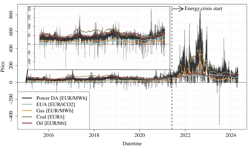
Figure 1: Price times series of German day-ahead power prices and front-month futures of EUA, gas, coal, oil.

1.1 Literature review

While there is an abundance of literature on short-term electricity price forecasting, research on mid to long-term forecasting remains relatively scarce, especially for an hourly resolution and for the energy crisis period in 2021-2023. [Ziel and Steinert, 2018] compiled an exhaustive list of papers covering econometric short, mid and long-term power price forecasting published between 2011 and 2017. Among these, only four papers, including the cited one, addressed long-term forecasting, while thirteen papers focused on mid-term forecasting. Here, mid-term refers to forecasting horizons from one month to one year ahead, while long-term refers to horizons beyond one year. We will be using this definition in this paper as well. Since then, more papers in this area have been published, but the literature remains notably limited.

For a new systematic literature overview, Tables 1 and 2 summarize papers found on mid-term to long-term forecasting since 2018. The papers were found using the Scopus search engine with queries as in [Ziel and Steinert, 2018], which can be found in the Appendix 6.1. We report five key aspects of each paper: the market, the forecasting horizon, the period covered, the regressors used, and the forecasting method. The tables show that the most common forecasting methods are autoregressive models, neural networks, and support vector machines. The most common regressors are autoregressive terms, with many papers not including external regressors at all. The markets covered are mainly European and US markets, with the most commonly ones being the PJM and ISO-NE regions in the US, Germany and the Iberian Electricity Market (MIBEL). The forecasting horizons range from one day to five years, with most papers focusing on horizons between one week and one month ahead. The periods covered range from 2002 to 2023, with most papers focusing on the years 2016-2021. Even recent papers tend to use data from before the 2021-2023 energy crisis.

Paper	Market	Horizon	Period	Regressors	Method
[Abroun et al., 2024]	Bulgaria, Greece, Hungary, Romania	1-7 months	2021-2022	Autoregressive	Nonlinear regression, neural networks, support vector regression
[Niafenderi and Mandal, 2023]	PJM (US)	1 day, 1 week	2006	Autoregressive	LSTM, convolutional neural networks
[Foroni et al., 2023]	Germany, Italy	1-28 days	2013-2020	Autoregressive, industrial production index, manufacturing performance indices, oil and gas prices	MIDAS regression
[Lee and Mandal, 2023]	PJM (US)	1 day, 1 week	2006	Autoregressive	Temporal convolutional neural networks
[Gomez et al., 2023]	PJM (US), Australia	2, 10, and 30 days	2020-2021	Autoregressive	LSTM, ensemble empirical mode decomposition
[Sgarlato and Ziel, 2022]	Germany	1-10 days	2020-2021	Autoregressive, coal, EUA, gas, meteorological data, weekday dummies	Lasso
[Wagner et al., 2022]	Germany	1 day, 4 years	2015-2019	Autoregressive, temperature, renewables infeed (for day-ahead only), weekdays, holidays	Neural networks
[Gabrielli et al., 2022]	UK, Germany, Sweden, Denmark	1 year	2015-2019	Autoregressive, power demand, generation, imports, renewables infeed, production from conventional plants, commodity prices	Linear regression, gaussian process regression, neural networks
[Karmakar et al., 2022]	Germany	1-17 weeks	2013-2014	Autoregressive	Robust Bayes, exponential smoothing state space models, neural networks, ARMAX
[Iqbal et al., 2022]	Australia	1,2 weeks	2020-2021	Autoregressive, load, infeed from renewables	Gated recurrent unit, bagged trees ensemble
[Irfan et al., 2022]	ISO-NE (US)	1 week	2017-2020	Autoregressive, load, temperature, weather	DenseNet neural networks,
[Ciarreta et al., 2022]	Germany, Austria	1-7 days	2016-2018	Autoregressive, weekday dummies, jump dummies	Lasso
[Aslam et al., 2021]	ISO-NE (US)	1-3 days, 1 week	2012-2020	Autoregressive, load, temperature, weather	Convolutional neural networks, XGBoost, Adaboost
[Matsumoto and Endo, 2021]	Japan	1 week	2016-2020	Autoregressive, temperature	Quantile regression, GARCH
[Teixeira et al., 2021]	MIBEL (Iberian Electricity Market)	1 month	2019-2020	Autoregressive	Artificial neural networks, extreme learning machines
[Imani et al., 2021]	Italy	1 hour, 1 day, 1 week	2020	Autoregressive, Load, natural gas	Support vector machines, tree-based methods, multilayer perceptron, gaussian process regression
[Spiliotis et al., 2021]	Belgium	1 week	2012-2016	Autoregressive, load, generation capacity, hour, year	Exponential smoothing, linear regression, multi-layer perceptron, random forest
[Ribeiro et al., 2020a], [Ribeiro et al., 2020b]	Brazil	1-3 months	2015-2020	Autoregressive, supply, demand	Coyote optimization, empirical mode decomposition, extreme learning machine, gaussian process, support vector regression, gradient boosting machine

Table 1: Papers covering mid and long-term forecasting of electricity prices from 2018 to 2020. Continued on Table 2.

Paper	Market	Horizon	Period	Regressors	Method
[Monteiro et al., 2020]	Iberian Electricity Market (MIBEL)	1-6 months	2018-2019	Autoregressive, delivery month, time to maturity, baseload physical power futures prices, spot price	Multilayer perceptron
[Yeardley et al., 2020]	UK	4 weeks	2017-2018	Autoregressive, demand, generation from conventional plants, renewables infeed	Gaussian process, clustering
[Česnavičius, 2020]	Lithuania	1 month	2020	Autoregressive	ARIMA, SARIMA
[Hammad-Ur-Rehman and Javaid, 2019]	NYISO (US)	1 day, 1 week	2016	Autoregressive	LDA, random forest, deep convoluted neural networks
[Windler et al., 2019]	Germany, Austria	1-29 days	2016	Autoregressive, hour/ day/ week/ month/ year dummies	Weighted nearest neighbors, exponential smoothing state space model, box-cox transformation, ARMA errors, trend and seasonal components (TBATS), deep neural networks
[de Marcos et al., 2019]	Iberian Electricity Market (MIBEL)	1 day, 1 week	2016	Autoregressive, fundamentally estimated market price, load, renewables infeed, seasonality dummies	Linear programming, artificial neural networks
[Razak et al., 2019]	Ontario (Canada)	1 month	2012	Autoregressive	Least square support vector machine, bacterial foraging optimization
[Ferreira et al., 2019]	Iberian Electricity Market (MIBEL)	1 month	2017	Autoregressive, electricity consumption/ imports/ exports, heating degree days, cooling degree days, macroeconomic indices, oil, renewables infeed	Linear regression
[Steinert and Ziel, 2019]	Germany	28 days	2016-2017	Autoregressive, base and peak daily/weekly/weekend/month futures, weekday dummies, periodic splines	Lasso
[Ali et al., 2019]	NYISO (US)	1 week	2014	Autoregressive, weather data, load	SVM, KNN, decision trees
[Yousefi et al., 2019]	California (US)	3, 5 years	2012-2017	Autoregressive, gas consumption, coal consumption, power generation/ imports, GDP, renewables infeed	LSTM, SARIMA
[Ubrani and Motwani, 2019]	India	1 day, 1 week	2017	Autoregressive	LSTM, gated recurrent unit
[Ma et al., 2018]	ERCOT (US)	1 month	2016	Autoregressive, prices of gas, nuclear, coal, renewables infeed, load, weather, power import/export, calendar days	Support vector machines
[Campos et al., 2018]	Spain, PJM (US)	1 day - 1 week	2002, 2006	Autoregressive	Wavelet transform, hybrid particle swarm optimization, adaptive neuro-fuzzy inference systems
[Razak et al., 2018]	Ontario (Canada)	1 month	2009-2010	Autoregressive	SVM, LSSVM, generic algorithm
[Marín et al., 2018]	Colombia	1 month	2014-2016	Autoregressive, hydro, availability	ARMAX, artifical neural networks
[Ziel and Steinert, 2018]	Germany	3 years	2015-2016	Autoregressive, temperature, renewables infeed, production from conventional plants, electricity load, auction data, day/week/season/holiday dummies	Lasso, supply and demand curve modeling

Table 2: Papers covering mid and long-term forecasting of electricity prices from 2018 to 2024. Continued from Table 1.

Some results of the query include papers that forecast day-ahead prices but refer to them as mid-term forecasts such as [Najafi et al., 2023], or as weekly forecasts as in [Aruldoss Albert Victoire et al., 2021]. Other papers do not focus on market power prices, such as [Yang, 2022] who analyze company-level prices, and other papers forecast day-ahead prices but analyze the long-term components as in [Jedrzejewski et al., 2021] and [Marcjasz et al., 2019], which is why they were returned by the query. We removed such papers from the list in the tables above and only included those that forecast market power prices for horizons higher than one day ahead.

The majority of papers focus on mid-term forecasting with forecasting horizons under a year, many under a month. Many studies model average monthly, weekly or yearly prices. None of the papers tackle forecasting power prices on an hourly basis around the energy crisis in 2021-2023 and the period thereafter.

1.2 Forecasting beyond day-ahead

Electricity price forecasting methods can be broadly classified into two categories: fundamental and data-driven models [Weron, 2014, Ziel and Steinert, 2016].

Fundamental models simulate the expected market conditions and power plant fleet within a geographic zone from which power prices are derived for example as shadow prices of the demand constraint. These models are typically used for long-term forecasting, as they require detailed information on the power plant fleet, fuel costs, and other market conditions. They are computationally expensive and deliver forecasts with low granularity, typically on a monthly or yearly basis. Furthermore, when employed for short-term forecasting, they are generally too flat and do not capture the high volatility of power prices [de Marcos et al., 2019], [Beran et al., 2021].

Econometric, machine-learning or, more generally, data-driven models utilize historical data to forecast power prices and are primarily employed for short-term forecasting, offering fine granularity ranging from minutes to hours [Weron, 2014, Ziel and Steinert, 2018, Narajewski and Ziel, 2020]. Having been extensively researched with various modelling approaches, important explanatory variables have been identified over the years. These include autoregressive terms that capture the recent past and inputs that can only be accurately forecasted in the short-term, such as renewables infeed. Such variables are crucial for day-ahead forecasting, but their explanatory power diminishes over longer horizons, making them less suitable for mid to long-term forecasting.

To illustrate, consider the following power price model, which includes variables that have been established to be most significant for day-ahead forecasting [Chai et al., 2023, Billé et al., 2023, Marcjasz et al., 2023, Maciejowska et al., 2020, Fezzi and Mosetti, 2020, Ziel and Weron, 2018, Uniejewski et al., 2017]:

$$\text{Price}_{t+h}= \beta_{0}+\underbrace{\beta_{1}\text{Mon}_{t+h}+\beta_{2}\text{Fri}_{t+h}+\beta_{3}\text{Sat}_{t+h}+\beta_{4}\text{Sun}_{t+h}}_{\text{Weekly seasonality}}$$ (1)

$$+\underbrace{\beta_{5}\text{Winter}_{t+h}+\beta_{6}\text{Spring}_{t+h}+\beta_{7}\text{Summer}_{t+h}}_{\text{Annual seasonality}}$$

$$+\underbrace{\beta_{8}\text{Price}_{t}+\beta_{9}\text{Price}_{t-1}+\beta_{10}\text{Price}_{t-6}+\beta_{11}\text{PriceLastHour}_{t}}_{\text{Autoregressive terms}}$$

$$+\underbrace{\beta_{12}\widehat{\text{RES}}_{t+1}+\beta_{13}\widehat{\text{Load}}_{t+1}}_{\text{Power market forecasts}}+\underbrace{\beta_{14}\text{EUA}_{t}+\beta_{15}\text{Gas}_{t}+\beta_{16}\text{Coal}_{t}+\beta_{17}\text{Oil}_{t}}_{\text{Commodity prices}}+\epsilon_{t}$$

where $h=1$ corresponds to forecasting one day ahead.

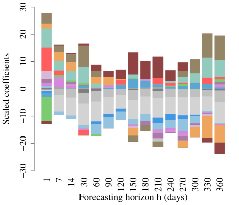
((a))

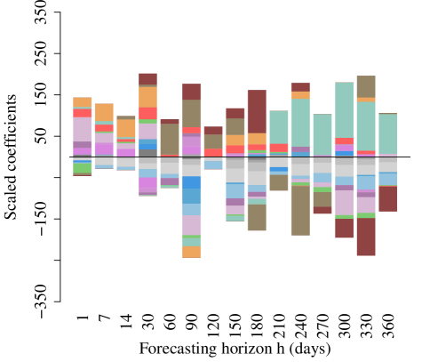
((b))

Figure 2: Scaled coefficients of model (1) for hour 9, for forecasting horizons from 1 to 360 days ahead, estimated using elastic net. Data from two periods were used to fit each model, before and after the energy crisis. Similar results were observed for all other hours.

Figure 2 depicts the estimated coefficients of this model across various forecasting horizons, ranging from one day to 360 days ahead, considering a representative day before and after the energy crisis. The estimates exhibit instability, particularly following the energy crisis and with increasing forecasting horizon $h$. For shorter horizons, the effects of renewables infeed, load, and autoregressive terms diminish rapidly, in line with expectations. However, they intermittently resurface at higher horizons without a discernible pattern. The coefficients of the commodity futures prices, representing fuel costs for conventional power plants, display strong offsetting effects. This phenomenon, where one coefficient is positive while the other is negative, thus partially offsetting each other, is a characteristic typical of highly correlated variables. Such effects are considered spurious, lacking a fundamental rationale. The only stable coefficients in the model are the deterministic terms, namely the weekly and annual seasonalities.

The research questions we aim to address in this paper are:

• What are the primary drivers of power prices beyond the day-ahead?

• How effectively do econometric models perform in such settings?

• What challenges do they encounter, and what are their limitations?

In doing so, we had to address the problems outlined above which resulted in three main novelties that our paper brings to the literature:

1. Inclusion of short-term regressors, such as renewables infeed, in long-term forecasts

2. Incorporating fundamental information based on energy economics theory

3. Addressing the unit root behavior of the power price, its drivers and implications for forecasting

From Tables 1 and 2 we can see that while some of these issues are addressed in a few papers, they are not considered as a whole. The provided solutions are often very specific to the pre-crisis period or the considered forecasting horizon, making it questionable if they remain robust when varying these two factors.

Regarding the inclusion of short-term regressors, [Ziel and Steinert, 2018] simulate wind and solar generation averages for long-term forecasts. [Gabrielli et al., 2022] use yearly wind and solar data. [Wagner et al., 2022] include renewables in short-term but not long-term forecasts. Other studies that focus on relatively short horizons up to a month simply use renewables as lagged regressors. We provide a method to incorporate short-term factors like renewables by estimating same-day relationships and projecting them arbitrarily far into the future using expected seasonal levels.

For incorporating fundamental information, [Gonzalez et al., 2011], [de Marcos et al., 2019], [Beran et al., 2021], and [Gabrielli et al., 2022] use hybrid models combining fundamental and econometric approaches. They generate power prices using market models and input these into econometric models. We incorporate fundamentally-derived information by setting coefficient bounds, stabilizing the model and reducing spurious effects.

Studies such as [Nowotarski and Weron, 2016], [Marcjasz et al., 2019], and [Jedrzejewski et al., 2021] examine long-term seasonal components of power prices for day-ahead forecasts, but do not address unit root behavior drivers and their implications for mid to long-term forecasting. We show that unit root behavior is explained by fuel commodity prices (gas, coal, oil, and emission allowances), though this diminishes with longer horizons, leading to spurious effects, especially during volatile periods like the energy crisis.

This paper is organized as follows. In the next section 2, we provide a brief overview of the data used in this study. In Section 2, we first present the basic electricity price model and the study design. We then analyse each of the aspects presented above and offer extensions of the basic model to address them. In Section 4 we summarize the considered models and report their forecasting accuracy. Based on these results, for forecasting horizons beyond 1 month ahead, we propose a model which we refer to as the ”current” model, which captures the same-day relationship between power price and its explanatory variables and projects it into the future. We conclude with a discussion of our findings and present directions for further research.

2 Data

The data we use for the model include hourly German day-ahead power prices, renewables infeed, load data, and commodity futures closing prices for EUA, gas, coal, and oil. The data spans 2015 to 2024 and is freely available on the ENTSOE Transparency platform, with the exception of the futures prices which were provided by the information platform Refinitiv Eikon. Figure 1 illustrates the day-ahead power and futures prices during this period, while Figure 3 presents the averages and standard deviations of power prices by year, season, week and hour.

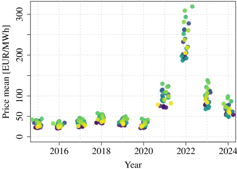
((a))

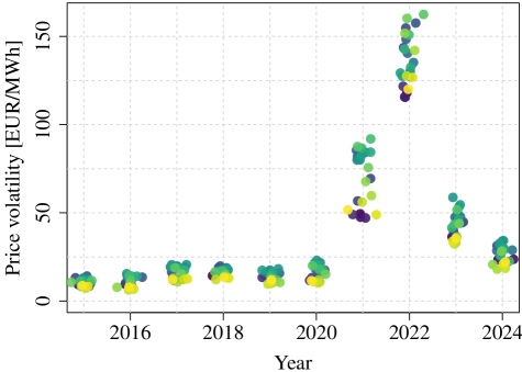
((b))

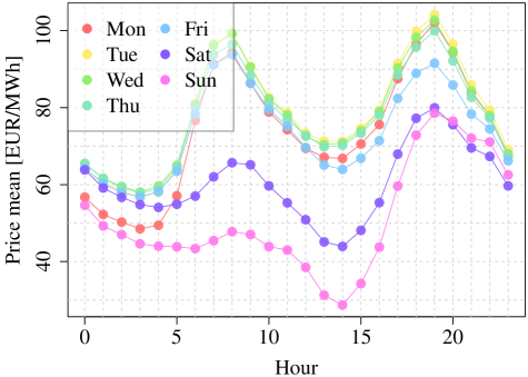
((c))

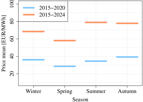
((d))

Figure 3: Statistics of German day-ahead power prices.

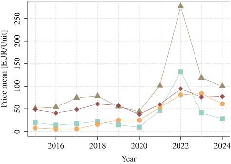
((a))

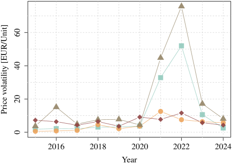
((b))

Figure 4: Statistics for front-month commodity futures prices: EUA, gas, coal, oil. (a) Mean and (b) standard deviation by year.

It is evident that, until 2020, power prices remained relatively stable around a mean of 40 EUR/MWh with their characteristic hourly, daily, weekly and annual seasonalities, as well as positive and negative price spikes. Prior to 2020, prices were characterized by lower volatility. However, during the energy crisis in 2021-2022, they experienced a significant surge, reaching over 800 EUR/MWh, before subsiding to a mean of around 100 EUR/MWh in 2023. It is widely documented in the literature that the crisis was triggered by a scarcity of gas supply in Europe, which in turn resulted from a combination geopolitical and economic events, such as the post-pandemic recovery, the Russia’s reduction of gas supply to Europe and the unfolding of the European Green Deal [Di Bella et al., 2022, Medzhidova, 2022, Szpilko and Ejdys, 2022, Emiliozzi et al., 2023].

Although price volatility reduced notably in 2023 compared to the heightened levels of 2021-2022, it still remains significantly elevated compared to pre-2020 levels. A similar pattern is observed in Figure 4 for the futures prices of EUA, gas, coal, and oil, which are highly correlated with power prices. As these commodities are used as fuels in the generation of electricity, their prices are key drivers of power prices. Indeed, their co-movement with the power prices is evident in the time series, especially for gas and coal. All data is available in hourly resolution, except for futures prices which are in daily resolution. We apply standard clock-change adjustment to the hourly data (interpolation in spring, averaging in fall).

3 Models

3.1 Basic model and study design

Model structures for short-term power price forecasting are well-researched and regressors with high explanatory power have been identified in the literature [Chai et al., 2023, Billé et al., 2023, Marcjasz et al., 2023, Maciejowska et al., 2020, Fezzi and Mosetti, 2020, Ziel and Weron, 2018, Uniejewski et al., 2017]. These models are referred to as expert models as they are current state-of-the art models with proven solid theoretic background and empirical backup [Weron and Ziel, 2019]. For day-ahead forecasts variables with high explanatory power include:

1. Deterministic terms: these include dummy variables and smooth periodic functions to capture daily, weekly and annual seasonal patterns,

2. Autoregressive terms: important lags were identified to be lags 1, 2 and 7, but complex models use autoregressive terms up to 30 days in the past,

3. Cross-period and non-linear price effects: these represent prices hours different than the one modelled, e.g. the last price of the previous day, or the highest and lowest prices of the previous day,

4. Day-ahead forecasts for infeed from renewable energy sources (RES),

5. Day-ahead forecasts of load,

6. Futures prices of gas, coal, emission allowances and oil.

Model (1) is a representative expert model which all of these regressors, except for the highest and lowest prices of the previous day.

The problems with model (1) were shown in the introduction and are obvious from Figure 2. The coefficients are as expected for the day-ahead forecast, but become unstable with increasing horizons and many apparently spurious effects can be observed. Hence the performance of the expert model is expected to decline drastically with increasing forecasting horizons. This prompts the question to what extend can an expert model structure be used for higher horizons. In the following sections we will discuss these problems and propose solutions to mitigate them.

Throughout this study we consider variations of model (1). For every considered model we conduct a rolling window forecasting study with a window size of $365\times 3$. Here the window size refers to the number of rows of the regressor matrix. In the $h=1$ case with autoregressive terms this corresponds to using the past 3 years of data for the model estimation. The window is rolled forward by one day after each forecast for an evaluation set of 6 years from April 2018 to April 2024. For each day 24 models are used, one for each hour of the day. Hence, at every rolling window step 24 models and sets of coefficients are estimated. We fit the models on normalized data using elastic net as implemented in the glmnet R package [Friedman et al., 2010, Simon et al., 2011, Tay et al., 2023]. The elastic net regularization parameter $\alpha$ is set to 0.5, which is a balanced mix of LASSO and ridge regression. The regularization parameter $\lambda$ is chosen using the Bayesian information criterion (BIC) from an exponential grid of $\lambda$. The models are evaluated using the mean absolute error (MAE) and the root mean squared error (RMSE) as performance measures.

3.2 Fundamental constraints for coefficients

One of the main problems with model (1) is that the sign of some estimated coefficients are not plausible from a theoretical point of view. For example, the coefficients of the commodity futures prices are expected to have a positive sign, as an increase in the price of the fuel used to generate electricity should lead to an increase in the power price [Everts et al., 2016, Bublitz et al., 2017, Hirth, 2018]. For the autoregressive terms positive coefficients are also expected, since high previous power prices should translate to high power prices in the short-term future, and low past prices to low future prices. Furthermore, according to the supply-stack model [He et al., 2013, Beran et al., 2019] the power supply curve is given by the marginal costs of available power plants sorted from lowest to highest. The power price is determined by the intersection of this supply curve with the inelastic power demand (load). Since renewables have marginal costs close to zero, power infeed from renewables effectively shifts the supply curve to the right thus decreasing the intersection price. Hence, the coefficient of renewable infeed should be negative. This is also referred to as the merit-order effect of renewables [Paraschiv et al., 2014, Dillig et al., 2016, Kolb et al., 2020, Gonçalves and Menezes, 2022]. Standard economic theory states that increasing demand increases the equilibrium price, hence the load coefficient should be positive. Figure 2 shows that, while these effects are as expected for short horizons, they are not consistent for longer horizons. This is especially obvious for the period that includes the energy crisis, where we see negative oil and coal coefficients even for the day-ahead forecast $h=1$.

Imposing this fundamentally motivated structure on the coefficients seems plausible and is straight-forward, as the coefficients have to be constrained to either positive or negative values as mentioned above. However, for the fuels coefficients we can not only set the lower bound to $0$ but also derive upper bounds. This is because the fuel coefficients essentially represent the conversion factors of the corresponding power plant. Since the units of the fuels differ from the unit of the power price the coefficients have an implicit unit that bridges the two. These are summarized in Table 3. Note that the units of the coefficients was chosen in such a way that the unit of the variable multiplied by the unit of the coefficient equals the unit of the power price (EUR/MWh). These units can now be used in combination with power plant efficiencies, CO2 intensity factors, and fuel conversion rates to derive upper bounds for the coefficients. These are summarized in Table 3 and are based on expert estimations from [Beran et al., 2019]. The efficiency factor $\eta$ is defined as the ratio of the electrical output power to the thermal input power, and the CO2 intensity factor $\varepsilon$ is defined as the ratio of the CO2 emissions to the thermal input power. The resulting bounds are summarized in Table 4.

Type	Units		Power Plant Characteristics
	Variable	Coefficient	Efficiency		CO2 factor	Ratio
			$\eta$ $\left[\frac{MWh_{el}}{MWh_{th}}\right]$		$\varepsilon$ $\left[\frac{tCO_{2}}{MWh_{th}}\right]$	$\frac{\varepsilon}{\eta}$ $\left[\frac{tCO_{2}}{MWh_{el}}\right]$
			Old	New		Old	New
Power	$\frac{\text{EUR}}{\text{MWh}_{el}}$	-	0.3	0.43	0.4	1.33	0.99
Lignite	$\frac{\text{EUR}}{\text{t}}$	-	0.3	0.43	0.4	1.33	0.99
Coal	$\frac{\text{EUR}}{\text{t}}$	$\frac{\text{t}}{\text{MWh}_{el}}$	0.35	0.46	0.3	0.86	0.65
Gas	$\frac{\text{EUR}}{\text{MWh}_{th}}$	$\frac{\text{MWh}_{th}}{\text{MWh}_{el}}$	0.25	0.4	0.2	0.8	0.5
Oil	$\frac{\text{EUR}}{\text{bbl}}$	$\frac{\text{bbl}}{\text{MWh}_{el}}$	0.24	0.44	-	-	-
EUA	$\frac{\text{EUR}}{\text{tCO}_{2}}$	$\frac{\text{tCO}_{2}}{\text{MWh}_{el}}$	-	-	-	-	-
Coal conversion	$1\ \text{t coal}=8,141\ \text{MWh}_{th}$
Oil conversion	$1,000\ \text{bbl oil}=1,700\ \text{MWh}_{th}$

Table 3: Units of variables and coefficients used in model (1). Power plant characteristics including efficiency and CO2-intensity factors for old and new power plants. Conversion factors for coal and oil. $\text{MWh}_{el}$ and $\text{MWh}_{th}$ stand for output and input power, respectively.

	Lags	Load	RES	EUA	Gas	Coal	Oil
Lower bound	$0$	$0$	$-\infty$	$0$	$0$	$0$	$0$
Upper bound	$\infty$	$\infty$	$0$	$1.33$	$4$	$0.123$	$0.588$

Table 4: Fundamentally-derived bounds for the coefficinets of selected regressors. All other coefficients are unbounded. The derivations can be found in the Appendix 6.2.

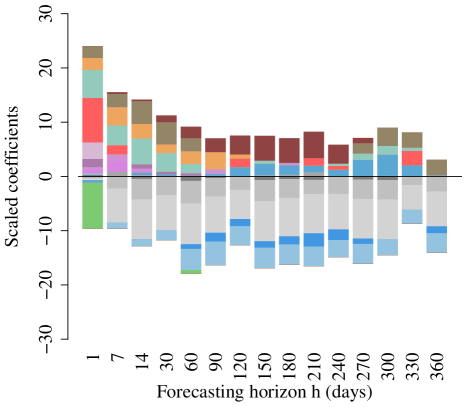
((a))

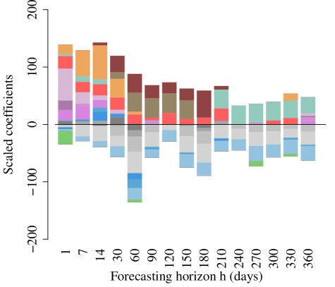
((b))

Figure 5: Scaled coefficients of the constrained model, i.e. model (1) with coefficient constraints in Table 4 for hour 9. Similar results were observed for all other hours.

Estimating model 1 using these bounds immediately results in more stable coefficients, in-line with the expected signs. These can be seen in Figure 5. The resulting stability is especially obvious for the right-hand side plot which includes the energy crisis. Some interesting dynamics can be observed. First, the coefficients of short-term regressors renewables, load and autoregressive terms diminish with increasing forecasting horizon as expected. Renewables becomes zero for 7 days ahead, while load becomes zero after 14 or 30 days for the pre- and post-crisis period respectively. The autoregressive terms vanish after 60 days for both periods. However, these terms still reappear at some higher horizons without clear patterns or magnitudes, hinting towards still remaining spurious effects. The coefficient estimates for commodity prices show distinct patterns. For shorter horizons, gas is predominant up to 120 days in the pre-crisis period and up to 30 days in the post-crisis period. As the horizon increases, coal becomes more relevant, particularly between 30 and 90 days. Oil gains importance for horizons between 90 and 210 days. The EUA coefficient is significant for short horizons, up to 60 days pre-crisis and 14 days post-crisis, then fades for mid horizons, and reemerges for horizons beyond 8 months pre-crisis and 6 months post-crisis. To summarize, gas, coal and EUA seem to be relevant for short forecasting horizons, while oil becomes relevant for mid to longer horizons up to 8 months ahead, after which only EUA is constantly active. For horizons beyond 8 months ahead the fuels seem to appear randomly without clear pattern, again indicating spurious effects.

3.3 Portfolio effects

In model (1), a single price for the commodities EUA, gas, coal, and oil was utilized, specifically the front-month futures closing prices. These prices represent the most recent monthly future closest to the time of forecasting. However, it’s crucial to note that various futures contracts exist for each commodity, spanning different maturities, including monthly, quarterly, and yearly futures. Figure 6 shows the price time series of futures for EUA, gas, coal, and oil with maturities from 1 to 12 months. It is immediately apparent that the futures are highly correlated, with lower maturity periods reacting more strongly to market changes and higher maturities following suit.

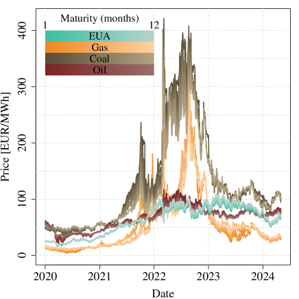
Figure 6: Price times series of 1 to 12-month futures.

Market participants, including electricity producers and buyers, do not only deal with front-month futures, but they also engage in longer-term futures. In practice, they often manage a portfolio of futures with various maturities for hedging or speculation purposes [Caldana et al., 2017, Steinert and Ziel, 2019].

For example, A power producer might hedge against potential gas price increases by taking a long position in a one-year future contract, thus securing a fixed price for future gas procurement. Often dynamic hedging is used, where producers adjust their fuel cost hedging as the delivery period approaches to mitigate price fluctuation risks. For instance, they might secure a 12-month gas future for 50% of their needs, a 6-month contract for another 25%, and a 3-month contract for the remaining 25%.

To examine portfolio effects, we extend model (1) by incorporating futures contracts with maturities up to 12 months ahead for each commodity. We include futures contracts with delivery periods $D$ corresponding to the forecast horizon’s month $m$. Additionally, we include futures contracts for the trailing month $D=m-1$ (one month before the delivery month) and the leading month $D=m+1$ (one month after the delivery month). The resulting model is the same as (1) but we replace each fuel price with the corresponding average lags, for example for gas we have:

$$\text{Price}_{t+h} =\beta_{0}+\dots+\sum_{i=m}^{12}\beta_{\text{Gas}D0,i}\overline{\text{Gas}}^{(D=m)}_{t-30i}+\sum_{i=m-1}^{12}\beta_{\text{Gas}D-1,i}\overline{\text{Gas}}^{(D=m-1)}_{t-30i}$$ (2)

$$+\sum_{i=m+1}^{12}\beta_{\text{Gas}D+1,i}\overline{\text{Gas}}^{(D=m+1)}_{t-30i}+\dots+\varepsilon_{t}$$

and for EUA, coal and oil equivalently, where $D$ indicates the delivery month of the future as of $t$ and $m=h/30$ is the delivery month corresponding to forecasting horizon $h$. The bar in $\overline{Gas}$ indicates that we take the monthly average of the futures prices where available. By calculating these averages, we presume that market participants hedge their fuel costs by continuously entering futures contracts throughout the month. Therefore, all futures prices within a given month influence the power price at delivery. It is important to note that the availability of futures contracts varies depending on the forecasting horizon and delivery period. For instance, when forecasting 30 days or 1 month ahead, the most recent available future for the delivery period in 1 month would be the front-month future with a lag of 1 month. For the trailing month, the most recent available price would be the front-month future with a lag of 2 months. For the leading month, the most recent available price would be the 2-month future with a lag of 1 month. Table 5 summarizes the lag structure of futures used for a specific forecasting horizon and their corresponding delivery month and lag.

Table 6 displays the resulting coefficients for pre- and post-energy crisis periods, respectively, for selected forecasting horizons. A noticeable pattern emerges with a preference for the most recent futures prices and lowest time to maturity for the pre-crisis period. Especially for day-ahead forecasts, the front-month futures, corresponding to a delivery period of the next month ($D+1$), are predominantly selected. Conversely, the most recent available futures for the current month ($D0$), with a lag of $0$, are almost entirely diminished to zero. Similar trends are observed for other forecasting horizons, where the most recent values, irrespective of their correspondence to the delivery period, are favored. While the effects in the post-crisis period are less pronounced, they remain discernible. Generally, the leading month seems most relevant for day-ahead forecasts, the delivery month for 30 days ahead, and the trailing month for other horizons. This finding is somewhat unexpected, as one would anticipate the delivery month to be most influential for all horizons due to physical fuel delivery. However, the results suggest that the most recent futures, regardless of their delivery period, hold more relevance for forecasting power prices. This observation aligns with the concept of an efficient market, where all available information is rapidly incorporated into the latest prices, resembling a Markov chain dynamic.

Horizon (days)	1	30	120	180	360	1	30	120	180	360	1	30	120	180	360
Horizon (months)	0	1	4	6	12	0	1	4	6	12	0	1	4	6	12
Lag	Delivery D0 maturity (months)					Delivery D-1 maturity (months)					Delivery D+1 maturity (months)
0											1
1	1	1									2	2
2	2	2				1	1				3	3
3	3	3				2	2				4	4
4	4	4	4			3	3	3			5	5	5
5	5	5	5			4	4	4			6	6	6
6	6	6	6	6		5	5	5	5		7	7	7	7
7	7	7	7	7		6	6	6	6		8	8	8	8
8	8	8	8	8		7	7	7	7		9	9	9	9
9	9	9	9	9		8	8	8	8		10	10	10	10
10	10	10	10	10		9	9	9	9		11	11	11	11
11	11	11	11	11		10	10	10	10		12	12	12	12
12	12	12	12	12	12	11	11	11	11	11

Table 5: Futures and their lag structure used as regressors for the portfolio model. They include the actual delivery period $D0$ in months, which corresponds to the forecast horizon, trailing delivery period $D-1$ and leading delivery period $D+1$.

Horizon (days)			1				30				120				180				360
Horizon (months)			0				1				4				6				12
Period	Delivery	Lag	Gas	Coal	EUA	Oil	Gas	Coal	EUA	Oil	Gas	Coal	EUA	Oil	Gas	Coal	EUA	Oil	Gas	Coal	EUA	Oil
2015-2019	D0	0	-	-	-	-	-	-	-	-	-	-	-	-	-	-	-	-	-	-	-	-
	D0	1	$0$	$0.019$	$0$	$0$	$0$	$0.332$	$0.076$	$0$	-	-	-	-	-	-	-	-	-	-	-	-
	D0	2	$0$	$0$	$0$	$0$	$0.046$	$0.015$	$0$	$0$	-	-	-	-	-	-	-	-	-	-	-	-
	D0	3	$0$	$0.003$	$0$	$0.004$	$0$	$0$	$0$	$0.044$	-	-	-	-	-	-	-	-	-	-	-	-
	D0	4	$0$	$0$	$0$	$0$	$0$	$0$	$0$	$0$	$0.059$	$0$	$0.002$	$0.018$	-	-	-	-	-	-	-	-
	D0	5	$0$	$0$	$0$	$0$	$0$	$0$	$0$	$0$	$0$	$0$	$0$	$0$	-	-	-	-	-	-	-	-
	D0	6	$0$	$0$	$0$	$0.003$	$0$	$0$	$0$	$0$	$0$	$0$	$0$	$0$	$0$	$0$	$0.009$	$0.001$	-	-	-	-
	D0	7	$0$	$0$	$0.003$	$0.002$	$0$	$0$	$0$	$0$	$0$	$0$	$0$	$0$	$0$	$0$	$0$	$0$	-	-	-	-
	D0	8	$0$	$0$	$0$	$0.001$	$0$	$0$	$0$	$0$	$0$	$0$	$0$	$0$	$0$	$0$	$0$	$0$	-	-	-	-
	D0	9	$0$	$0$	$0.047$	$0$	$0$	$0$	$0$	$0$	$0$	$0$	$0$	$0$	$0$	$0$	$0$	$0$	-	-	-	-
	D0	10	$0$	$0$	$0$	$0$	$0$	$0$	$0$	$0$	$0$	$0$	$0$	$0$	$0$	$0$	$0$	$0$	-	-	-	-
	D0	11	$0$	$0$	$0.006$	$0$	$0$	$0$	$0.007$	$0$	$0$	$0$	$0$	$0$	$0$	$0$	$0$	$0$	-	-	-	-
	D0	12	$0$	$0$	$0.185$	$0$	$0$	$0$	$0.456$	$0$	$0$	$0$	$0$	$0$	$0$	$0$	$0$	$0$	$0$	$0.004$	$0$	$0$
	D-1	0	-	-	-	-	-	-	-	-	-	-	-	-	-	-	-	-	-	-	-	-
	D-1	1	-	-	-	-	-	-	-	-	-	-	-	-	-	-	-	-	-	-	-	-
	D-1	2	$0$	$0.067$	$0$	$0$	$0$	$0.223$	$0$	$0.001$	-	-	-	-	-	-	-	-	-	-	-	-
	D-1	3	$0$	$0$	$0$	$0.001$	$0$	$0$	$0$	$0.123$	-	-	-	-	-	-	-	-	-	-	-	-
	D-1	4	$0$	$0$	$0$	$0$	$0$	$0$	$0$	$0$	$0.317$	$0$	$0.028$	$0.326$	-	-	-	-	-	-	-	-
	D-1	5	$0$	$0$	$0$	$0$	$0$	$0$	$0$	$0$	$0$	$0$	$0$	$0$	-	-	-	-	-	-	-	-
	D-1	6	$0.039$	$0$	$0$	$0.003$	$0$	$0$	$0$	$0$	$0$	$0$	$0$	$0$	$0$	$0$	$0.075$	$0.296$	-	-	-	-
	D-1	7	$0.14$	$0$	$0$	$0.006$	$0$	$0$	$0$	$0.01$	$0$	$0$	$0$	$0$	$0$	$0$	$0$	$0.021$	-	-	-	-
	D-1	8	$0.015$	$0$	$0$	$0.005$	$0$	$0$	$0$	$0$	$0$	$0$	$0$	$0$	$0$	$0$	$0$	$0$	-	-	-	-
	D-1	9	$0$	$0$	$0$	$0$	$0$	$0$	$0$	$0$	$0$	$0$	$0$	$0$	$0$	$0$	$0$	$0$	-	-	-	-
	D-1	10	$0$	$0$	$0$	$0$	$0$	$0$	$0$	$0$	$0$	$0$	$0$	$0$	$0$	$0$	$0$	$0$	-	-	-	-
	D-1	11	$0$	$0$	$0.003$	$0$	$0$	$0$	$0$	$0$	$0$	$0$	$0$	$0$	$0$	$0$	$0$	$0$	-	-	-	-
	D-1	12	$0$	$0$	$0.085$	$0$	$0$	$0$	$0.153$	$0$	$0$	$0$	$0$	$0$	$0$	$0.049$	$0$	$0$	$0$	$0.273$	$0$	$0$
	D+1	0	$0.479$	$0.14$	$0.197$	$0.008$	-	-	-	-	-	-	-	-	-	-	-	-	-	-	-	-
	D+1	1	$0$	$0$	$0$	$0.026$	$0$	$0.099$	$0.08$	$0.098$	-	-	-	-	-	-	-	-	-	-	-	-
	D+1	2	$0$	$0$	$0$	$0.007$	$0.04$	$0$	$0$	$0.026$	-	-	-	-	-	-	-	-	-	-	-	-
	D+1	3	$0$	$0.02$	$0$	$0.155$	$0$	$0$	$0$	$0.111$	-	-	-	-	-	-	-	-	-	-	-	-
	D+1	4	$0.002$	$0$	$0$	$0$	$0$	$0$	$0$	$0$	$0.124$	$0$	$0$	$0$	-	-	-	-	-	-	-	-
	D+1	5	$0$	$0$	$0$	$0$	$0$	$0$	$0$	$0$	$0$	$0$	$0$	$0$	-	-	-	-	-	-	-	-
	D+1	6	$0.02$	$0$	$0$	$0.036$	$0$	$0$	$0$	$0$	$0$	$0$	$0$	$0$	$0$	$0$	$0$	$0$	-	-	-	-
	D+1	7	$0.029$	$0$	$0$	$0.005$	$0$	$0$	$0$	$0$	$0$	$0$	$0$	$0$	$0$	$0.007$	$0$	$0$	-	-	-	-
	D+1	8	$0.003$	$0$	$0$	$0.022$	$0$	$0$	$0$	$0$	$0$	$0$	$0$	$0$	$0$	$0.022$	$0$	$0$	-	-	-	-
	D+1	9	$0$	$0$	$0.007$	$0.001$	$0$	$0$	$0$	$0$	$0$	$0$	$0$	$0$	$0$	$0$	$0$	$0$	-	-	-	-
	D+1	10	$0$	$0$	$0$	$0$	$0$	$0$	$0$	$0$	$0$	$0$	$0$	$0$	$0$	$0$	$0$	$0$	-	-	-	-
	D+1	11	$0$	$0$	$0$	$0$	$0$	$0$	$0.072$	$0$	$0$	$0$	$0$	$0$	$0$	$0$	$0$	$0$	-	-	-	-
	D+1	12	-	-	-	-	-	-	-	-	-	-	-	-	-	-	-	-	-	-	-	-
2020-2024	D0	0	-	-	-	-	-	-	-	-	-	-	-	-	-	-	-	-	-	-	-	-
	D0	1	$0$	$0$	$0.014$	$0.008$	$0.307$	$0.024$	$0.033$	$1.617$	-	-	-	-	-	-	-	-	-	-	-	-
	D0	2	$0$	$0$	$0$	$0$	$0$	$0$	$0$	$0$	-	-	-	-	-	-	-	-	-	-	-	-
	D0	3	$0$	$0$	$0$	$0$	$0$	$0$	$0$	$0$	-	-	-	-	-	-	-	-	-	-	-	-
	D0	4	$0$	$0$	$0$	$0$	$0$	$0$	$0$	$0$	$0$	$0$	$0$	$0.212$	-	-	-	-	-	-	-	-
	D0	5	$0$	$0$	$0$	$0$	$0$	$0$	$0$	$0$	$0$	$0$	$0$	$0$	-	-	-	-	-	-	-	-
	D0	6	$0$	$0$	$0$	$0$	$0$	$0$	$0$	$0$	$0$	$0$	$0$	$0$	$0$	$0$	$0$	$0.019$	-	-	-	-
	D0	7	$0$	$0$	$0.027$	$0$	$0$	$0$	$0$	$0$	$0$	$0$	$0$	$0$	$0$	$0$	$0$	$0$	-	-	-	-
	D0	8	$0$	$0$	$0$	$0$	$0$	$0$	$0$	$0$	$0$	$0$	$0$	$0$	$0$	$0$	$0$	$0$	-	-	-	-
	D0	9	$0$	$0$	$0$	$0$	$0$	$0$	$0$	$0$	$0$	$0$	$0$	$0$	$0$	$0$	$0$	$0$	-	-	-	-
	D0	10	$0$	$0$	$0$	$0$	$0$	$0$	$0$	$0$	$0$	$0$	$0$	$0$	$0$	$0$	$0$	$0$	-	-	-	-
	D0	11	$0$	$0$	$0$	$0$	$0$	$0$	$0$	$0$	$0$	$0$	$0$	$0$	$0$	$0$	$0$	$0$	-	-	-	-
	D0	12	$0.021$	$0.002$	$0$	$0$	$0$	$0$	$0$	$0$	$0$	$0$	$0$	$0$	$0$	$0$	$0$	$0$	$0$	$0$	$0.882$	$0$
	D-1	0	-	-	-	-	-	-	-	-	-	-	-	-	-	-	-	-	-	-	-	-
	D-1	1	-	-	-	-	-	-	-	-	-	-	-	-	-	-	-	-	-	-	-	-
	D-1	2	$0$	$0$	$0$	$0$	$0$	$0.164$	$0$	$0.416$	-	-	-	-	-	-	-	-	-	-	-	-
	D-1	3	$0$	$0$	$0$	$0$	$0$	$0$	$0$	$0$	-	-	-	-	-	-	-	-	-	-	-	-
	D-1	4	$0$	$0$	$0$	$0$	$0.001$	$0$	$0$	$0$	$0$	$0.229$	$0$	$1.306$	-	-	-	-	-	-	-	-
	D-1	5	$0$	$0$	$0$	$0$	$0$	$0$	$0$	$0$	$0$	$0.003$	$0$	$0$	-	-	-	-	-	-	-	-
	D-1	6	$0$	$0$	$0.01$	$0$	$0$	$0$	$0$	$0$	$0$	$0$	$0$	$0$	$0$	$0$	$0.02$	$1.212$	-	-	-	-
	D-1	7	$0$	$0$	$0.018$	$0$	$0$	$0$	$0$	$0$	$0$	$0$	$0$	$0$	$0$	$0$	$0.566$	$0$	-	-	-	-
	D-1	8	$0$	$0$	$0$	$0$	$0$	$0$	$0$	$0$	$0$	$0$	$0$	$0$	$0$	$0$	$0$	$0$	-	-	-	-
	D-1	9	$0$	$0$	$0$	$0$	$0$	$0$	$0$	$0$	$0$	$0$	$0$	$0$	$0$	$0$	$0$	$0$	-	-	-	-
	D-1	10	$0$	$0$	$0$	$0$	$0$	$0$	$0$	$0$	$0$	$0$	$0$	$0$	$0$	$0$	$0$	$0$	-	-	-	-
	D-1	11	$0$	$0$	$0$	$0$	$0$	$0$	$0$	$0$	$0$	$0$	$0$	$0$	$0$	$0$	$0$	$0$	-	-	-	-
	D-1	12	$0.002$	$0$	$0$	$0$	$0$	$0$	$0$	$0$	$0$	$0$	$0$	$0$	$0$	$0$	$0$	$0$	$0$	$0$	$1.3$	$0$
	D+1	0	$0.357$	$0$	$0.185$	$0$	-	-	-	-	-	-	-	-	-	-	-	-	-	-	-	-
	D+1	1	$0$	$0$	$0.012$	$0$	$0$	$0$	$0$	$0$	-	-	-	-	-	-	-	-	-	-	-	-
	D+1	2	$0$	$0$	$0$	$0$	$0$	$0$	$0$	$0$	-	-	-	-	-	-	-	-	-	-	-	-
	D+1	3	$0$	$0$	$0$	$0$	$0$	$0$	$0$	$0$	-	-	-	-	-	-	-	-	-	-	-	-
	D+1	4	$0$	$0$	$0$	$0$	$0$	$0$	$0$	$0$	$0$	$0$	$0$	$0$	-	-	-	-	-	-	-	-
	D+1	5	$0$	$0$	$0$	$0$	$0$	$0$	$0$	$0$	$0$	$0$	$0$	$0$	-	-	-	-	-	-	-	-
	D+1	6	$0$	$0$	$0$	$0$	$0$	$0$	$0$	$0$	$0$	$0$	$0$	$0$	$0$	$0$	$0$	$0$	-	-	-	-
	D+1	7	$0$	$0$	$0$	$0$	$0$	$0$	$0$	$0$	$0$	$0$	$0$	$0$	$0$	$0$	$0$	$0$	-	-	-	-
	D+1	8	$0$	$0$	$0$	$0$	$0$	$0$	$0$	$0$	$0$	$0$	$0$	$0$	$0$	$0$	$0$	$0$	-	-	-	-
	D+1	9	$0$	$0$	$0$	$0$	$0$	$0$	$0$	$0$	$0$	$0$	$0$	$0$	$0$	$0$	$0$	$0$	-	-	-	-
	D+1	10	$0$	$0$	$0$	$0$	$0$	$0$	$0$	$0$	$0$	$0$	$0$	$0$	$0$	$0$	$0$	$0$	-	-	-	-
	D+1	11	$0.005$	$0$	$0$	$0$	$0$	$0$	$0$	$0$	$0$	$0$	$0$	$0$	$0$	$0$	$0$	$0$	-	-	-	-
	D+1	12	-	-	-	-	-	-	-	-	-	-	-	-	-	-	-	-	-	-	-	-

Table 6: Average fuels coefficients of the portfolio model for two periods. $D0$, $D-1$, and $D+1$ are the actual, trailing and leading delivery periods.

3.4 Short-term regressors

As evident in Figure 5, the coefficients of renewable energy infeed and load in model (1) decrease rapidly with increasing forecasting horizons. This is particularly evident for the pre-2020 period in Figure 5.a, aligning with fundamental expectations. In the post-2020 period illustrated in Figure 5.b, load appears relevant until approximately 60 days ahead after which the coefficient becomes unstable. Consequently, these short-term explanatory variables become ineffective for forecasting purposes as their corresponding coefficients become essentially zero. However, solar and wind production as well as load demonstrate robust annual seasonalities, the expected levels of which can be forecasted. These seasonal patterns are illustrated in Figure 7. The forecasts were generated using Generalized Additive Models (GAMs) as implemented in the mgcv R package [Wood, 2011, Wood et al., 2016, Wood, 2004, 2017, 2003] with formulas as shown in Equation (6.3) in the Appendix.

Figure 7.a depicts the renewables infeed modeled and forecasted as the sum of wind and solar production. The impact of solar infeed is immediately evident: first, in the daily cycle with higher values during the day and lower values during the night hours, and second, in the annual cycle with higher values during the summer months and lower values during the winter months. The wind infeed exhibits less pronounced daily and annual cycles but still demonstrates a clear pattern with a peak in winter and spring, and during nighttime hours. These interactions of wind and PV seasonalities result in complex multi-modal fit curves that can nevertheless be extrapolated arbitrarily far into the future. A linear trend component is included in the model to capture the expected expansion of renewables capacity. Figure 7.b shows the daily, weekly, and annual cycles of the load, with higher values during working hours and during winter, and lower values during the night, weekends, holidays, and summer. This pattern is also expected to persist into the future. The fact that the linear trend component for load has a negative slope could indicate increasing power efficiency in the market or the outsourcing of industrial processes outside of Germany. Comparing the two figures, it is evident that renewables infeed fluctuates significantly more than load, with extreme jumps from one day to the next. This is due to the fact that renewables infeed is highly dependent on weather conditions, which can change rapidly [Sgarlato and Ziel, 2022]. In contrast, load is more stable, primarily driven by human behavior.

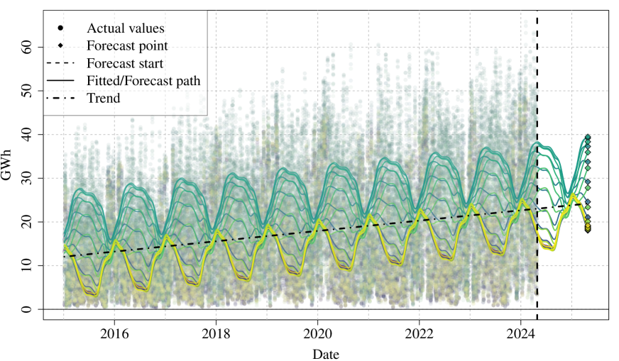
((a))

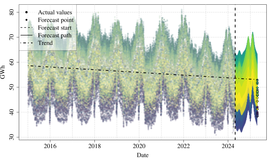
((b))

Figure 7: The forecast was generated using Generalized Additive Models (GAMs).

It is reasonable to assume that the power price is influenced by these seasonal changes. For instance, higher solar irradiation during summer is likely to exert a greater downward pressure on power prices compared to winter, when irradiance levels are substantially lower. Therefore, a model with estimated zero coefficients for load and renewables would fail to capture such effects. While zero-coefficient estimations are theoretically accurate, as day-ahead renewables infeed and load forecasts are not expected to have significant explanatory power for forecasts beyond the day-ahead, they the overlook seasonal impact. Ideally, we would have $h$-ahead forecasts of renewables infeed and load to incorporate into the model. However, such forecasts are unavailable, and even if they were, they would only provide seasonal expectations and would not capture unforeseen shocks, particularly for renewables infeed. Consequently, the estimation algorithm tends to shrink the corresponding coefficients toward zero, especially for longer forecasting horizons.

Therefore, we propose a method to integrate the anticipated levels of renewables infeed and load for all forecasting horizons into the model. This is achieved by initially estimating the relationship between the power price and renewables infeed/load for the same day. Consequently, for the estimation, model (1) is adapted to:

$$\text{Price}_{t+h}=\beta_{0}+\dots+\underbrace{\beta_{12}\text{RES}_{\color[rgb]{0.8,0,0}{t+h}}+\beta_{13}\text{Load}_{\color[rgb]{0.8,0,0}{t+h}}}_{\text{Power market forecasts}}+\dots$$ (3)

and the corresponding forecast is calculated as:

$$\widehat{\text{Price}}_{T+h}=\beta_{0}+\dots+\underbrace{\beta_{12}\widehat{\text{RES}}_{\color[rgb]{0.8,0,0}{T+h}}+\beta_{13}\widehat{\text{Load}}_{\color[rgb]{0.8,0,0}{T+h}}}_{\text{Power market forecasts}}+\dots$$ (4)

This effectively captures the impact of renewables infeed and load levels on the power price, as if we had perfect forecasts for estimation. As observed in Figure 8, the coefficients of renewables infeed and load become highly relevant for all forecasting horizons. Consequently, in some cases, the coefficients for weekend dummies may become positive. Initially, this may seem counterintuitive since prices typically decrease on Saturdays and Sundays compared to weekdays. However, this weekend effect primarily arises from load, as demand is lower on weekends. Since load is controlled for in this model, the weekend effect is implicitly captured, thus the weekend variables must be interpreted as capturing a weekend effect not solely driven by the demand side. The observation that the coefficients for weekend dummies are mostly zero or close to zero suggests that the weekend effect is predominantly driven by the demand side, with no additional effect on the supply side. Moreover, weekends and load are negatively correlated, as load is consistently lower on weekends than on weekdays. Therefore, the presence of positive weekend dummies could potentially represent another spurious effect arising from highly correlated variables.

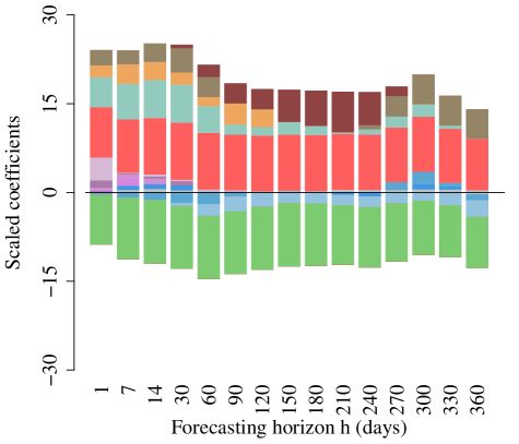
((a))

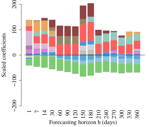
((b))

Figure 8: Scaled coefficients of the ”short-term” model 3 for hour 9. Similar results were observed for all other hours.

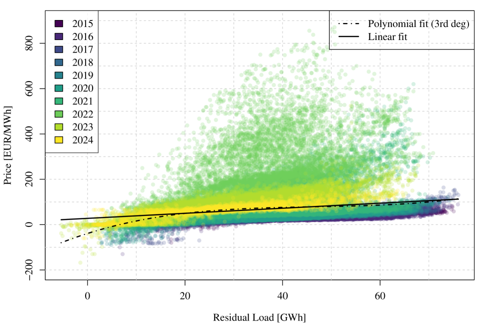
Figure 14: Residual load and day-ahead power prices in Germany by year. The fitted curve is a third-degree polynomial of residual load: $\text{Price}_{t}=\beta_{0}+\beta_{1}\text{ResLoad}_{t}+\beta_{2}\text{ResLoad}_{t}^{2}+\beta_{3}\text{ResLoad}_{t}^{3}+\varepsilon_{t}$. Linear fit for comparison. Note that the linear fit approximates the non-linear fit well, except for the portion of extreme negative prices.

It is evident that $\text{RES}_{T+h}$ and $\text{Load}_{T+h}$ are unavailable when forecasting the power price $\text{Price}_{T+h}$. Therefore, for forecasting purposes, we replace renewables infeed and load with their forecasts $h$ days ahead, which are seasonal expectations as shown in Figure 7, while keeping the coefficients estimated on same-day data. Consequently, the power price is trained on actual data while the forecast is conditioned on the expected seasonal level of renewables. This approach offers the advantage of capturing the actual effects of renewables infeed and load on the price while also incorporating future developments such as expansion of renewables capacity or power efficiency improvements. The relationship between Price and residual load is non-linear in nature (see Figure 14), however incorporating non-linear effects such as second and third degree polynomials leads to a small impact of the non-linear parts and do not seem to improve the power price forecasting accuracy.

3.5 Unit root behavior

3.5.1 Effects of stochastic trends

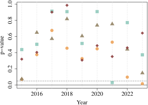
((a))

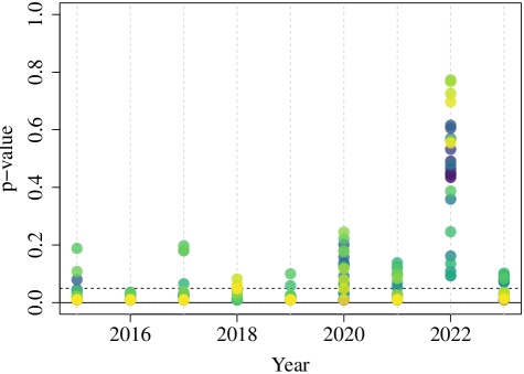
((b))

Figure 17: p-values of augmented Dickey-Fuller (ADF) unit root test with the alternative hypothesis ”stationarity”, for (a) EUA, gas, coal and oil front month futures prices by year and for (b) German day-ahead power prices by hour and year. The dashed horizontal line represents the 0.05 significance level. The results must be interpreted with care as the underlying assumptions of the ADF test might be questionable for the data at hand.

A widely accepted fact in finance is that stock prices exhibit unit root behavior, indicating that they are non-stationary and possess a stochastic trend to some degree. This assumption is evident in the modeling of stocks as Brownian motions, also referred to as Gaussian or Wiener processes, or functions thereof for structuring and valuation purposes, such as pricing derivatives [Black and Scholes, 1973, Schwartz and Smith, 2000, Hull, 2009]. This unit-root behavior extends to commodities like EUA, gas, coal, and oil [Schwartz and Smith, 2000]. In fact, unit root tests for these futures prices fail to reject the null hypothesis of having a unit root (see Figure 17) [Berrisch et al., 2023].

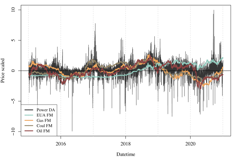
Figure 13: Scaled price times series of German day-ahead power prices and front-month futures for EUA, gas, coal, oil for the period 2015-2020.

Since these commodities lack obvious seasonalities or deterministic effects, forecasting them differs from renewables or load. Futures prices thus provide the only available future-oriented information. Additionally, as fuels for power generation, it is reasonable to assume that the power price inherits some unit root behavior from them, particularly visible in the long run (see Figure 13 in the Appendix). Indeed, visual inspection of power price time series in Figure 1 suggests some stochastic trend, which towards the end of 2021 broke out of its historic mean-reverting behavior. However, unlike other commodity prices, the electricity price also manifests strong deterministic components, such as daily, weekly, and yearly seasonalities (see Figure 3), alongside well-known causal effects like the merit order effect of renewables.

Moreover, the challenge intensifies with increasing forecasting horizons due to two main simultaneously occurring effects:

Firstly, the stochastic component gains prominence. With a higher forecasting horizon, the price can deviate more from its current value due to its stochastic trend. In such cases, it becomes feasible to forecast only the deterministic components, such as trend and seasonality. However, if the stochastic component is exceptionally volatile, it could potentially obscure such deterministic effects, especially if they are weak. Some evidence of this phenomenon can be observed in Figure 3.(d), where, on average, the price in summer appears slightly lower than in winter and autumn due to higher PV infeed. Indeed, this effect is noticeable when examining the seasonal averages before 2021. However, due to the power price surge that commenced in mid-2021 and peaked in mid-2022, when considering the average inclusive of this period, summer prices appear to be the highest, leading to the loss of the annual effect. Indeed, in the short run the trend of the power price is well captured by the fuels prices, but with an increasing forecasting horizon, the fuels can not explain the trend anymore, since the trend is driven by future values of the fuels prices which are not known at the time of forecasting.

Secondly, we encounter a loss of explanatory variables. Short-term causal variables, such as renewables infeed and load, lose their predictive power with increasing forecasting horizon [Weron and Ziel, 2019]. This effectively creates a gap in explaining the response, thereby leaving the estimation procedure struggling to filter out causal effects, that could be partly or completely obscured by a stochastic trend, with even less explanatory power.

3.5.2 Effects of unit-root regressors

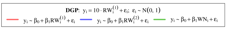
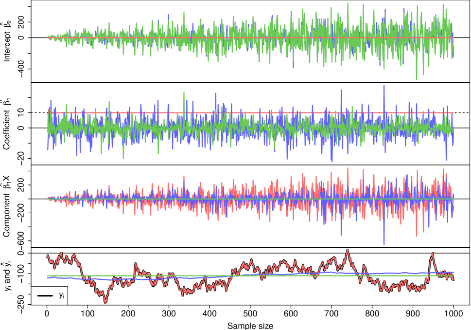
Figure 16: Estimated coefficients, components and a sample path, for increasing sample size showcasing 3 cases when the response $y$ has a random walk component: a. regression on a random walk $RW^{(1)}$ that is part of the data generating process (DGP) (red); 2. regression on a random walk $RW^{(2)}$ that is not part of the DGP (blue); and 3. regression on white noise $WN$ that is not part of the DGP (green).

Furthermore, the inclusion of commodity futures prices as explanatory variables for the power price carries important statistical implications. Specifically, if regressors lacking explanatory power are included, the chance of spurious effects is considerably higher compared to non-unit root regressors [Granger and Newbold, 1974, Lütkepohl, 2005]. It can be demonstrated that when regressing a random walk on an unrelated regressor, the OLS estimator becomes inconsistent both in terms of intercept and slope. This inconsistency arises because the martingale difference condition is violated by the error term. This is illustrated in a simple simulation in Figure 16. Moreover, if the regressor is also a random walk, the resulting component $X\beta$ will exhibit increasing variance with the sample size, hence a larger sample size would not be beneficial. In contrast, if a white noise is used as a regressor, most of the fit will be captured by the intercept, and the corresponding component will not have a variance increasing with the sample size.

Indeed, this effect can be observed in our real-life setting in Figure 9. If we include randomly generated discrete brownian motions and white noises into model (1), we observe that the corresponding coefficients are not always shrunk to zero, especially for higher horizons and for the period after the energy crisis. In the second plot this effect is apparently highly significant, as the coefficients of the brownian motions are very high. This is a clear indication that the model is struggling to filter out the stochastic trend from the regressors, and the resulting coefficients are not only spurious, but also inconsistent. Intuitively, when the coefficients of the brownian motions have at least the same magnitute as those of the non-deterministic components, the relevance of those components is highly questionable.

It could be considered that the power price and fuels prices are cointegrated, as they do seem to move together in the long run to a certain extend [Moutinho et al., 2022]. However, the cointegration relationship might be complex and might change both over time due to complex effects such as fuel switches and supply-stack non-linearities. Furthermore, with an increasing forecasting horizon the model approaches the case of a classical spurious regression case when a unit root process is regressed on another independent unit root process [Granger and Newbold, 1974]. In such a case, where the forecasting horizon is large, it is unlikely that a long-term equilibrium relationship even exists between power price and fuels. Lastly, our 24-dimensional model structure, where we model each hour individually, and the usage of external regressors does not fit in the classical framework of cointegration and vector error correction models, making standard statistical tests and theory unapplicable in our context.

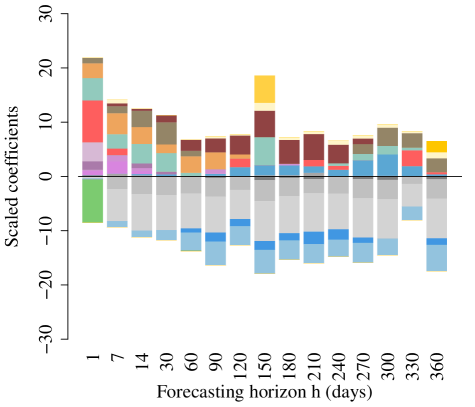
((a))

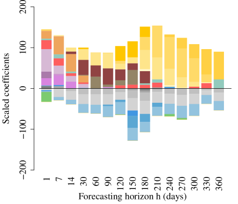
((b))

Figure 9: Scaled coefficients of the constrained model (1) with 4 randomly generated brownian motions and white noises as regressors, for hour 9.

3.5.3 Differentiation

Differencing is a well-known technique in time series analysis used to eliminate a unit root trend and render the time series stationary [Brockwell and Davis, 2002, Hamilton, 2020]. This technique forms the basis for ARIMA-based models. Differencing model (1) implies applying the difference operator $\Delta$, where $\Delta y_{t}=y_{t}-y_{t-1}$, to the whole equation, including the response and all regressors. The model is then estimated as:

$$\Delta\text{Price}_{t+h} =\beta_{1}\Delta\text{Mon}_{t+h}+\dots+\beta_{8}\Delta\text{Price}_{t}+\dots$$ (5)

$$\Leftrightarrow(\text{Price}_{t+h}-\text{Price}_{t+h-1}) =\beta_{1}(\text{Mon}_{t+h}-\text{Mon}_{t+h-1})+\dots+\beta_{8}(\text{Price}_{t}-\text{Price}_{t-1})+\dots$$

and forecasted as

$$\widehat{\Delta\text{Price}}_{T+h} =\widehat{\beta}_{1}\Delta\text{Mon}_{T+h}+\dots+\widehat{\beta}_{8}\Delta\text{Price}_{T}+\dots$$ (6)

$$\widehat{\text{Price}}_{T+h} =\text{Price}_{T}+\widehat{\Delta\text{Price}}_{T+h}.$$

We note that $\Delta$ represents the one-period differencing operator, yet the forecasting gap between the response and regressors remains the forecasting horizon $h$.

Indeed, if the power price exhibits an unexplained unit root trend, differencing could potentially improve the forecast. However, if the unit root behavior in the price is accounted for by at least one of the regressors, differencing is not expected to yield significant improvement. Empirical results seem to confirm this hypothesis. Table 7 displays the forecasting accuracies in terms of yearly RMSE for selected forecasting horizons with and without differencing, when fuels prices are included as regressors compared to when they are not. Table 11 in the Appendix also shows the corresponding MAE (see section 4). Similar results are observed for both RMSE and MAE. To isolate the unit-root regressors from the non-unit ones, we omitted the annual components and load for this comparison, recognizing that load might have an underlying stochastic trend [Smyth, 2013].

Horizon	1				90				180				360
Model	No fuels		Fuels		No fuels		Fuels		No fuels		Fuels		No fuels		Fuels
Diff	No	Yes	No	Yes	No	Yes	No	Yes	No	Yes	No	Yes	No	Yes	No	Yes
2018	8.84	7.75	7.17	7.77	20.25	21.72	17.65	21.64	22.34	26.67	21.62	26.55	23.99	26.28	24.00	26.27
2019	9.37	9.32	8.55	9.33	13.73	21.44	16.48	21.35	13.68	23.68	17.43	23.63	14.34	22.79	14.51	22.79
2020	8.38	8.73	7.94	8.72	16.36	22.40	19.97	22.28	17.25	25.25	20.28	25.20	16.15	22.36	17.30	22.37
2021	29.98	30.19	29.11	30.23	71.53	67.79	62.81	67.75	91.38	83.37	92.62	83.35	92.76	95.41	97.60	95.43
2022	55.72	55.96	54.60	55.94	213.56	201.35	159.06	202.02	186.59	178.01	165.02	178.06	253.16	199.91	245.72	199.91
2023	25.80	25.03	24.32	24.94	73.03	94.74	105.49	94.70	280.55	179.53	247.55	179.21	609.41	197.80	576.04	197.93
2024	22.91	26.64	25.67	26.52	58.23	54.84	77.64	54.78	71.60	58.26	138.29	57.98	119.13	68.55	162.18	68.44

Table 7: Yearly RMSE (EUR/MWh) out-of-sample showing effect of differencing with and without fuels as regressors for selected forecasting horizons.

The findings indicate that differencing sometimes enhances forecasting accuracy when fuels are not included, particularly for short forecasting horizons such as day-ahead. When fuels are included, differencing does not add any benefit for day-ahead forecasts. This provides evidence that power prices indeed exhibit some unit root behavior, as they benefit from differencing. Moreover, it suggests that this stochastic trend is explained by fuels prices. For longer horizons, differencing begins to improve forecasting accuracy even when unit-root regressors are included. This is expected as the stochastic trend becomes more pronounced with increasing forecasting horizon, and there is a lack of explanatory variables. Even including fuels futures cannot fully explain the stochastic trend between the last known value at $T$ and the forecast $T+h$.

3.5.4 Current fit

We have seen that the presence of a gap between the response and regressors poses a significant challenge when extending forecasts beyond the day ahead. This gap allows the stochastic trend to influence the relationship, complicating estimation and potentially leading to spurious correlations, particularly evident during periods of strong stochastic trends like in 2022. While day-ahead forecasts are less affected due to the limited time for price drift and the explanatory power of fuel prices, addressing spurious effects and maintaining causal relationships becomes paramount when extending forecasts. One approach to mitigate this issue involves separating the estimation and forecasting processes, akin to what was done for short-term regressors in (3). In this approach, estimation utilizes current-day values to capture the structural relationship between price and regressors. Then, in a subsequent step, the response is forecasted by substituting the regressors with their forecasts. Precisely, the temporal relationship between the response and regressors during training differs from that during forecasting. During training, same-day values are utilized to establish the relationship, while forecasting involves incorporating the temporal aspect into the relationship. Essentially, the same-day relationship is implicitly expected to persist into the future. This method helps maintain causal relations and reduces the chance of spurious effects in extended forecasts.

Thus, for the estimation, model (1) is modified to:

$$\text{Price}_{t+h}=\dots+\underbrace{\beta_{14}\text{EUA}^{\text{(01)}}_{\color[rgb]{0.8,0,0}{t+h}}+\beta_{15}\text{Gas}^{\text{(01)}}_{\color[rgb]{0.8,0,0}{t+h}}+\beta_{16}\text{Coal}^{\text{(01)}}_{\color[rgb]{0.8,0,0}{t+h}}+\beta_{17}\text{Oil}^{\text{(01)}}_{\color[rgb]{0.8,0,0}{t+h}}}_{\text{Commodity prices}}+\epsilon_{t}$$ (7)

where $(01)$ represents the front-month future, which is the most recent price. The corresponding forecast is calculated as:

$$\widehat{\text{Price}}_{T+h}=\dots+\underbrace{\beta_{14}\text{EUA}_{T}^{\color[rgb]{0.8,0,0}{\text{(m)}}}+\beta_{15}\text{Gas}_{T}^{\color[rgb]{0.8,0,0}{\text{(m)}}}+\beta_{16}\text{Coal}_{T}^{\color[rgb]{0.8,0,0}{\text{(m)}}}+\beta_{17}\text{Oil}_{T}^{\color[rgb]{0.8,0,0}{\text{(m)}}}}_{\text{Commodity prices}}+\epsilon_{t}$$ (8)

where $m=h/30$ represents the delivery month corresponding to the forecasting horizon.

Hence, we always use the front month to estimate the coefficients for EUA, gas, coal, and oil. For generating forecasts, we plug in the front-month futures into the model for a 30-day ahead forecast, the second-month future price for a 60-day ahead forecast, and so forth, while keeping the estimated coefficients unchanged. The coefficients estimated from this model are depicted in Figure 10. Notably, oil is not present in any of the horizons, and coal is absent from the right-hand-side plot. This contrasts with previous models where coal and oil were relevant for mid to long-term horizons. The absence of oil aligns with the scarcity of oil power plants in Germany. Gas, on the other hand, emerges as a significant factor, particularly evident in the second plot, signifying its pivotal role as a price-setting technology during the power price surge in the energy crisis. Although coal also surged during 2021-2022, its correlation with the power price appears weaker compared to gas.

These findings suggest that gas functions as a short-term regressor with substantial explanatory power in the short run. Moreover, the relevance of oil only becomes apparent as we introduce the temporal dimension between response and regressor, indicating that oil may serve as a proxy for gas in the long run, suggesting a potential predictive relationship between oil and gas prices.

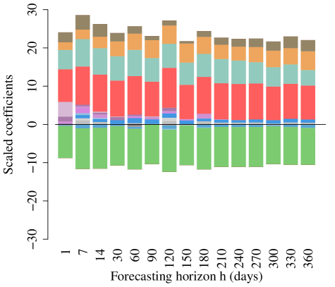
((a))

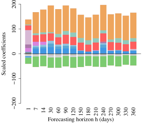
((b))

Figure 10: Scaled coefficients of the ”current” model 7 for hour 9. Similar results were observed for all other hours.

4 Results

In the previous section we introduced several models for forecasting power prices. These are summarized in Table 8.

Model	Model equation	Summary
No constraints	Eq. (1)	Expert model with no constraints.
Constrained	Eq. (1) & Table 4	Expert model with fundamental constraints on coefficients.
Constrained diff	Eq. (1) & Eq. (5)	Constrained model with differenced response and regressors.
Portfolio	Eq. (1) & Eq. (2)	Constrained model with up to 12 fuels futures for delivery, trailing and leading month to forecasting horizon.
Short-term	Eq. (1) & Eq. (3)	Constrained model with same-day coefficient estimates for RES and Load, and seasonal expectations for prediction.
Current	Eq. (1) & Eq. (3) & Eq. (7)	Short-term model with same-day regressors for fuels futures, with futures corresponding to the forecasting horizon for prediction.

Table 8: Models considered.

For evaluation we use the mean absolute error (MAE) and the root mean squared error (RMSE) as performance metrics. They are defined as:

$$\text{MAE}(\varepsilon)=\frac{1}{24N}\sum_{i=1}^{N}\sum_{h=1}^{24}|\widehat{\varepsilon}_{T+i,h}|\text{ and }\text{RMSE}(\varepsilon)=\sqrt{\frac{1}{24N}\sum_{i=1}^{N}\sum_{h=1}^{24}\widehat{\varepsilon}_{T+i,h}^{2}}$$

where $\widehat{\varepsilon}_{t,h}$ is the forecasting error at time $t$ for hour $h$.

Model/Horizon	1	7	14	30	60	90	120	150	180	210	240	270	300	330	360
No constr	24.17	$41.80$	$48.09$	$60.54$	$61.65$	$74.79$	$78.44$	$90.10$	$109.35$	$133.67$	$144.68$	$147.96$	$183.76$	$208.04$	$187.91$
Constr	$24.18$	41.13	46.96	$56.00$	60.14	$70.16$	$79.17$	$88.18$	$102.57$	$113.28$	$130.57$	$141.83$	$155.23$	$169.16$	$178.46$
Constr diff	$26.68$	$50.68$	$56.10$	$65.31$	$72.64$	$77.20$	$80.69$	$87.39$	$91.38$	$91.98$	$93.19$	$94.56$	$98.19$	$97.42$	$101.30$
Portfolio	$24.22$	$43.05$	$52.10$	$63.20$	$70.94$	$84.13$	$91.14$	$94.61$	$104.06$	$112.67$	$124.37$	$133.84$	$150.27$	$152.68$	$173.51$
Short-term	$29.09$	$43.70$	$49.43$	$57.22$	$61.28$	$70.43$	$80.05$	$91.68$	$104.85$	$116.07$	$129.96$	$140.33$	$157.15$	$176.12$	$186.45$
Current	$29.09$	$43.59$	$47.80$	54.36	$60.37$	66.34	72.86	76.16	80.56	86.16	90.07	88.68	94.17	96.37	97.29

Table 9: RMSE (EUR/MWh) for the evaluation period April/2018-April/2023 for all considered models and forecasting horizons over all 24 hours.

Year	Model/Horizon	1	7	14	30	60	90	120	150	180	210	240	270	300	330	360
2018	No constr	$6.44$	$13.06$	$13.07$	$14.06$	$17.08$	$20.81$	$27.98$	$24.49$	$28.56$	$28.53$	$24.58$	$23.61$	$26.17$	$24.63$	$24.39$
	Constr	$6.43$	12.95	12.98	13.62	15.40	17.46	18.90	19.91	$21.12$	$21.55$	21.86	$21.99$	$22.42$	$22.03$	21.71
	Constr diff	$7.35$	$17.33$	$18.04$	$17.99$	$20.75$	$21.67$	$20.87$	$24.74$	$26.61$	$26.87$	$27.23$	$27.07$	$26.96$	$25.75$	$26.38$
	Portfolio	6.37	$13.64$	$14.20$	$16.20$	$19.67$	$22.26$	$19.72$	$20.16$	20.70	21.33	$21.92$	21.91	22.04	21.77	$21.71$
	Short-term	$10.83$	$13.41$	$13.59$	$14.34$	$15.97$	$18.44$	$20.49$	$21.87$	$22.78$	$23.40$	$23.87$	$24.32$	$24.34$	$24.28$	$24.07$
	Current	$10.83$	$13.51$	$13.86$	$14.86$	$16.36$	$17.54$	$19.41$	$20.83$	$21.46$	$22.02$	$22.35$	$22.49$	$22.58$	$22.82$	$22.90$
2019	No constr	7.65	$12.48$	$12.94$	$13.11$	$13.52$	14.66	$17.39$	$26.46$	$22.65$	$23.13$	$27.82$	$29.76$	$30.90$	$40.79$	$29.47$
	Constr	$7.65$	12.44	12.93	13.07	13.30	$14.71$	$16.04$	$17.55$	$17.93$	$17.00$	$18.69$	$17.53$	15.35	14.17	13.89
	Constr diff	$9.52$	$17.76$	$18.37$	$19.77$	$20.79$	$21.44$	$21.11$	$24.25$	$23.65$	$22.79$	$23.59$	$24.43$	$23.45$	$21.84$	$22.94$
	Portfolio	$7.81$	$13.16$	$14.14$	$15.10$	$15.63$	$19.22$	$19.50$	$21.19$	$21.15$	$28.13$	$23.90$	$18.41$	$16.51$	$14.71$	$14.34$
	Short-term	$11.47$	$13.36$	$13.67$	$13.95$	$14.15$	$15.57$	$17.32$	$18.70$	$18.29$	$18.21$	$18.96$	$18.32$	$16.22$	$14.88$	$15.32$
	Current	$11.47$	$13.31$	$13.65$	$13.75$	$14.30$	$14.82$	15.21	15.94	16.07	15.54	15.62	15.67	$15.73$	$15.80$	$15.85$
2020	No constr	$7.32$	$12.23$	$12.71$	$13.38$	14.64	$16.72$	$19.03$	$18.77$	$19.16$	$19.93$	$18.55$	$19.60$	$21.65$	$31.91$	$39.15$
	Constr	7.26	12.20	12.67	13.30	$14.66$	$16.68$	$18.62$	$17.93$	$17.67$	$17.17$	$16.91$	$16.99$	$16.56$	16.29	15.06
	Constr diff	$8.89$	$16.75$	$17.69$	$19.44$	$21.35$	$22.35$	$21.72$	$24.90$	$25.22$	$24.52$	$23.98$	$24.06$	$22.06$	$18.97$	$22.44$
	Portfolio	$7.49$	$12.92$	$13.62$	$14.83$	$16.65$	$17.41$	$18.44$	17.48	17.48	16.93	16.81	16.67	16.49	$16.62$	$16.12$
	Short-term	$11.65$	$13.24$	$13.68$	$14.43$	$15.99$	$18.16$	$18.54$	$19.43$	$19.41$	$18.55$	$17.69$	$17.42$	$17.53$	$17.80$	$16.31$
	Current	$11.65$	$13.27$	$13.74$	$14.53$	$15.31$	16.34	17.65	$18.13$	$19.10$	$19.41$	$19.35$	$19.56$	$19.54$	$19.42$	$19.93$
2021	No constr	28.46	$51.95$	$52.99$	$55.38$	46.76	54.09	63.53	$79.53$	$97.29$	$101.18$	$100.35$	$100.18$	$97.81$	$96.70$	$96.40$
	Constr	$28.65$	$48.23$	$51.41$	$52.84$	$48.42$	$58.07$	$69.43$	$82.97$	$90.70$	$91.81$	$92.11$	$92.37$	$93.30$	$94.08$	$95.18$
	Constr diff	$31.13$	$56.69$	$59.04$	$57.45$	$64.11$	$67.74$	$77.46$	$79.95$	$83.37$	$86.91$	$88.83$	$91.52$	90.83	92.14	$95.43$
	Portfolio	$28.47$	47.10	48.24	47.82	$47.32$	$57.82$	$70.36$	$85.26$	$91.27$	$92.29$	$92.54$	$92.57$	$92.79$	$92.15$	91.79
	Short-term	$34.20$	$48.96$	$52.33$	$54.56$	$51.41$	$61.71$	$72.35$	$85.86$	$93.96$	$95.48$	$95.84$	$95.57$	$95.86$	$96.66$	$97.73$
	Current	$34.20$	$48.85$	$52.04$	$55.04$	$57.98$	$67.92$	$75.10$	78.77	82.20	84.69	87.45	89.28	$91.23$	$92.45$	$93.52$
2022	No constr	52.77	$106.09$	$127.55$	$151.04$	$152.97$	149.65	143.58	$171.23$	$151.19$	$176.08$	$219.28$	$259.91$	$327.38$	$327.53$	$254.37$
	Constr	$53.32$	105.07	$124.73$	144.68	152.78	$159.26$	$168.33$	$161.13$	$168.15$	$190.28$	$208.52$	$208.74$	$214.88$	$223.28$	$229.21$
	Constr diff	$57.87$	$119.59$	$141.00$	$171.84$	$197.96$	$201.85$	$189.49$	$173.30$	$178.09$	$173.30$	179.82	178.59	194.18	195.90	199.86
	Portfolio	$53.84$	$113.99$	$141.30$	$160.43$	$179.79$	$167.42$	$152.10$	150.36	148.65	159.29	$185.98$	$218.16$	$231.29$	$224.93$	$229.02$
	Short-term	$61.95$	$105.56$	$124.47$	$145.32$	$153.90$	$156.13$	$164.41$	$157.02$	$163.76$	$188.80$	$206.83$	$203.88$	$214.70$	$224.50$	$231.59$
	Current	$61.95$	$107.40$	123.39	$148.17$	$174.89$	$178.71$	$172.98$	$151.63$	$159.36$	$171.54$	$179.99$	$192.19$	$205.56$	$210.60$	$214.53$
2023	No constr	$24.34$	$41.70$	$51.91$	$86.43$	$92.27$	$138.91$	$159.99$	$184.79$	$209.19$	$228.56$	$248.81$	$301.81$	$423.87$	$563.42$	$450.42$
	Constr	23.76	41.14	$50.35$	$74.04$	$81.62$	$107.31$	$138.71$	$191.30$	$234.20$	$282.84$	$359.04$	$425.41$	$496.39$	$557.25$	$576.03$
	Constr diff	$25.16$	$53.86$	$56.48$	$83.83$	$84.17$	$94.85$	$115.74$	$160.98$	$179.64$	$186.09$	190.78	$193.27$	$204.16$	$199.63$	$198.74$
	Portfolio	$23.82$	$43.78$	$65.06$	$103.62$	$121.17$	$171.25$	$207.97$	$218.06$	$237.80$	$260.66$	$297.31$	$329.26$	$395.10$	$386.38$	$486.66$
	Short-term	$31.60$	$45.38$	$54.23$	$73.90$	$80.93$	$104.48$	$134.91$	$189.14$	$235.19$	$287.71$	$363.54$	$426.95$	$511.01$	$602.18$	$618.62$
	Current	$31.60$	$42.58$	45.91	55.50	61.44	80.32	113.90	146.90	159.18	179.36	$195.34$	168.87	182.06	187.28	180.66
2024	No constr	$24.46$	26.34	$30.44$	$43.90$	$49.72$	$74.73$	$67.09$	$59.81$	$156.62$	$253.16$	$253.26$	$176.51$	$200.97$	$187.88$	$257.62$
	Constr	$24.46$	$27.71$	29.68	$38.05$	$50.07$	$64.90$	$63.89$	$58.21$	$86.75$	$80.58$	$88.18$	$89.93$	$94.92$	$109.86$	$141.36$
	Constr diff	$27.52$	$39.41$	$44.03$	$39.56$	$47.47$	$55.00$	$58.60$	$60.93$	$58.31$	$58.27$	$52.15$	$55.52$	$54.46$	$56.05$	$68.36$
	Portfolio	$23.87$	$27.34$	$30.22$	37.42	$45.11$	$71.64$	$78.49$	$75.30$	$108.00$	$118.71$	$129.70$	$127.99$	$149.45$	$181.27$	$203.14$
	Short-term	23.69	$35.69$	$38.20$	$41.15$	$51.28$	$66.51$	$72.76$	$79.94$	$98.47$	$87.65$	$76.91$	$79.82$	$87.60$	$100.70$	$139.12$
	Current	$23.69$	$36.13$	$38.07$	$39.16$	38.27	39.96	42.30	45.57	47.45	46.43	42.68	46.49	50.88	52.69	59.27

Table 10: Yearly RMSE (EUR/MWh) for the evaluation period April/2018-April/2023 for all considered models and forecasting horizons over all 24 hours.

The overall evaluation RMSE is shown in Table 9. The MAE is shown in the appendix in Table In Tables 12. It becomes evident that the current model consistently outperforms all other models for forecasting horizons beginning at 30 days or one month ahead. This marks the point where capturing the relationship between variables becomes more important than incorporating the temporal dimension. Essentially, the information between $T+h$ and $T$ ceases to enhance the forecast compared to solely extrapolating the current relationship between the response and regressor into the future. This signifies a manifestation of the martingale property for the power price, where the last available value proves to be the best forecast.

However, when examining the errors for each year individually in Tables 10 for RMSE and 13 for MAE, the distinction is less clear. During periods of stable prices, such as in 2018-2020, the constrained model often performs the best. Conversely, during the energy crisis in 2022, the differentiated constrained model excels for higher horizons. This suggests that the ability of an econometric model to extract information from the temporal relationship between response and regressors depends on the stability of power price dynamics. Nonetheless, the outperformance of the current model compared to others on average indicates that the martingale property is a characteristic of power price dynamics. Given that we have seen the tendency of the models to fit spurious effects for higher horizons, the results suggest that the current model is the most robust choice.

Additionally, we can analyze the drivers of the power price by examining the components of the forecasts. Figure 11 displays the contributions of the regressors to the forecasts, i.e. the regressor multiplied by the coefficient, for two selected weeks before and after the energy crisis. The sum of the components at each time point equals the forecast. The upper two graphs illustrate the day-ahead forecasts and their components for the ”constrained” model, which performed the best in the day-ahead setting. The middle and lower graphs depict the forecasts based on the ”current” model. Various expected effects are observable, such as the night-hours and weekend effects, with lower prices during the night and weekends driven mainly by lower load. The impact of the last hour of yesterday is most relevant for early night hours due to its temporal closeness. Furthermore, the merit order effect is evident, where high renewables infeed, especially wind, leads to small or even negative prices. The typical lower prices during mid-day, driven by high solar infeed, are also observable. Additionally, we can see the price-setting powerplant effect, with gas usually being the more expensive fuel. Gas power plants are price-setting during peak hours, resulting in lower contributions of gas during base hours and higher contributions during peak hours. In the post-energy crisis period, we observe no contribution from coal, indicating that the gas price was the main driver for the power price dynamics during that time. For horizons beyond day-ahead, accurately forecasting renewables shocks is not possible. Therefore, the renewables area always represents the expected seasonal infeed. The same applies for load.

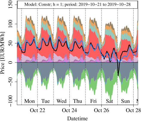
((a))

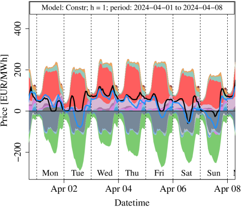
((b))

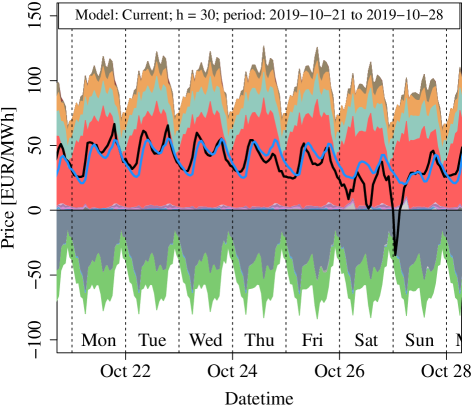
((c))

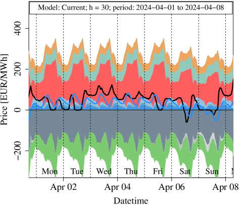
((d))

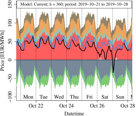
((e))

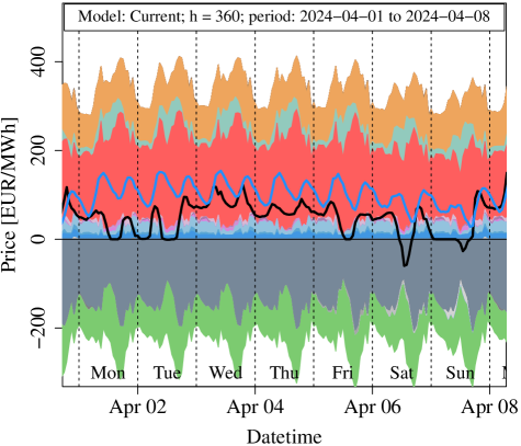
((f))

Figure 11: Price forecasts and their components for selected models and periods.

To better understand why some models perform better than others for certain horizons we can look at the forecasts of the considered models for the period 2021-2024, as shown in Figure 12. The left plot depicts day-ahead forecasts, while the right one displays year-ahead forecasts, showing both ends of the considered forecasting spectrum. For the day-ahead forecasts, the models exhibit some similarities, but the current model appears to have difficulty capturing the range and volatility as effectively as the others. This is because, similar to the short-term model and unlike the rest of the models, it does not make use of day-ahead forecasts for renewables and load thus failing to predict price spikes both positive and negative. Table 12 confirms that the current model performs relatively poorly for day-ahead forecasts, while the model using fundamental constraints performs the best.

However, in the right plot, we observe that all models except for the differencing and current models significantly overshoot the prices in 2023. For instance, the constrained and short-term models predict prices exceeding 2000 EUR/MWh in the summer of 2023. This discrepancy arises because these forecasts were generated in the summer of 2022, a year prior, when prices were very high. Due to the substantial temporal gap between response and regressor, the estimation procedure had to explain this price surge using data from 2021, which were substantially lower. Extrapolating this trend into the future leads to the observed overshooting effect. We note that this effect is not a-priori undesirable or incorrect, as at the time of forecasting it was not known that the prices would drop in 2023. At that time the scenario where prices would have continued to rise up to the possible limits set by the fundamental constraints was not implausible, which would have made such forecasts more accurate.

Differentiation mitigates the overshooting effect to a significant extent, yet the model displays marked volatility, extrapolating the high volatility observed in 2022 into 2023. On the other hand, the current model does not exhibit these effects, as it only captures the current relationship between response and regressor and projects it into the future. Consequently, the current model returns forecasts resembling a rightward shift of the true price time series.

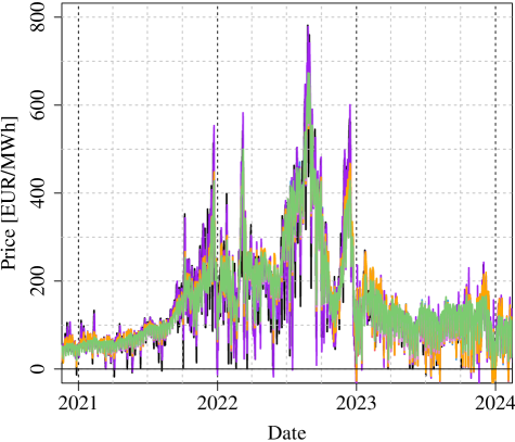
((a))

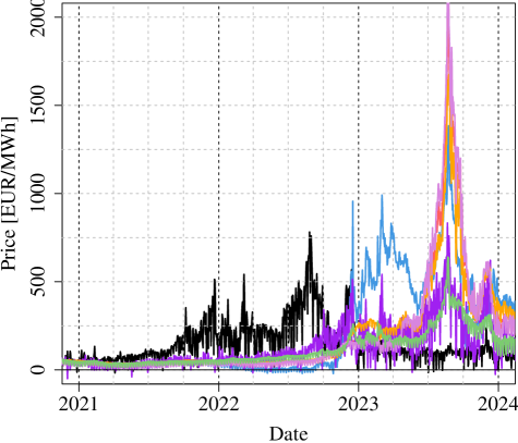
((b))

Figure 12: Forecasts of considered models for 2021-2024 for hour 9. Similar results were observed for all other hours.

5 Summary and conclusion

We presented the challenges associated with mid-term and long-term power price forecasting using econometric models, highlighting issues such as coefficient instability and the increasing importance of the stochastic component with longer forecasting horizons. Notably, we showed that the long-term unit root behavior of power prices can be explained by prices of commodities that are used as fuels to produce power, including emission allowances (EUA), gas, coal, and oil. However, the explanatory power of these commodities diminishes significantly as the forecasting horizon extends. During unstable periods, such as the 2022 energy crisis, we demonstrated that including randomly generated Brownian motions as explanatory variables can result in them being incorrectly identified as highly relevant. This indicates spurious effects and overfitting due to the unit root behavior of both the power price and the regressors.

To mitigate coefficient instabilities, we proposed a constrained model that restricts the coefficients within fundamental bounds derived from power plant efficiencies, CO2 intensity factors, and fuel conversion rates. We also examined the portfolio effects of different futures contracts and found that power prices are most influenced by the most recent contracts, without clearly discernible portfolio patterns.

To address the spurious effects caused by the stochastic trend of power prices, we proposed the ”current” model. In this model, the price is fitted to current-day values of the regressors, and for forecasting, this relationship is extrapolated into the future by inputting expected future values of the regressors. This model outperformed all other models for forecasting horizons starting from 30 days ahead on average, suggesting that beyond approximately one month ahead, capturing the actual relationship between the response and the regressor becomes more important than incorporating the temporal dimension by lagging the response and regressors. This finding aligns with the martingale property of efficient market theory, where the last available value is the best forecast. However, performance varies by year: the constrained model often performed best during stable periods, while the differentiated constrained model excelled during the 2022 energy crisis. The current model provided good forecasts for 2023 and 2024, indicating that the best model depends on the current regime of power prices.

The model could be extended to include probabilistic forecasts. This could be done by simulating future values of the regressors, particularly commodity prices, while accounting for their correlation or cointegration relationships, and calculating the resulting power price distribution. Sampling residuals conditioned on specific values of the regressors could also generate probabilistic forecasts.

Further research could focus on extending the model to incorporate more complex relationships between the regressors and power prices, such as interactions between different fuels. This would account for effects like fuel switches, where two or more fuels change order in the supply stack model. Achieving this would require an in-depth exploration of fundamental power market theory and its intersection with econometric models, along with a detailed analysis of the merit order model and its estimation. Another area of further reasearch could be the expansion of cointegration theory and vector error correction models to allow for a 24-hour model, where each hour is modelled in a separate equation, as well as for the usage of external regressors. This could allow better capturing of the relationship between power price and fuel commodities, and potentially offer deeper insight into unit root behavior for longer forecasting horizons.

Declaration of Generative AI and AI-assisted technologies

During the preparation of this work the authors used GitHub Copilot and OpenAI ChatGPT-3.5 in order to generate rephrasing suggestions to improve the language and readability of this paper. After using this tool/service, the authors reviewed and edited the content as needed and take full responsibility for the content of the publication.

6 Appendix

6.1 Scopus Queries

• Scopus query for papers covering mid-term forecasting:

(TITLE(((((”electric*” OR ”energy market” OR ”power price” OR ”power market” OR ”power system” OR pool OR”market clearing” OR ”energy clearing”) AND (price OR prices OR pricing)) OR lmp OR ”locational marginal price”) AND (forecast OR forecasts OR forecasting OR prediction OR predicting OR predictability OR ”predictive densit*”)) OR (”price forecasting” AND ”smart grid*”)) OR TITLE-ABS(”electricity price forecasting” OR ”forecasting electricity price” OR ”day-ahead price forecasting” OR ”day-ahead mar* price forecasting” OR (gefcom2014 AND price) OR ((”electricity market” OR ”electric energy market”) AND ”price forecasting”) OR (”electricity price” AND (”prediction interval” OR ”interval forecast” OR ”density forecast” OR ”probabilistic forecast”))) AND NOT TITLE (”unit commitment”)) AND ( TITLE(”mid-term”) OR TITLE(”mid term”) OR TITLE(”medium-term”) OR TITLE(”medium term”) OR TITLE(”long-term”) OR TITLE(”long term”) OR TITLE-ABS-KEY(”mid-term electric*”) OR TITLE-ABS-KEY(”mid term electric*”) OR TITLE-ABS-KEY(”medium-term electric*”) OR TITLE-ABS-KEY(”medium term electric*”) OR TITLE-ABS-KEY(”long-term electric*”) OR TITLE-ABS-KEY(”long term electric*”) OR TITLE-ABS-KEY(”mid-term price*”) OR TITLE-ABS-KEY(”mid term price*”) OR TITLE-ABS-KEY(”medium- term price*”) OR TITLE-ABS-KEY(”medium term price*”) OR TITLE-ABS-KEY(”weeks-ahead”) OR TITLE-ABS-KEY(”weeks ahead”) OR TITLE-ABS-KEY(”month-ahead”) OR TITLE-ABS-KEY(”month ahead”) OR TITLE-ABS-KEY(”mid term* horizon”) OR TITLE-ABS-KEY(”mid-term* horizon”) OR TITLE-ABS-KEY(”medium term* horizon”) OR TITLE-ABS-KEY(”medium-term* horizon”))

• Scopus query for papers covering long-term forecasting:

(TITLE(((((”electric*” OR ”energy market” OR ”power price” OR ”power market” OR ”power system” OR pool OR”market clearing” OR ”energy clearing”) AND (price OR prices OR pricing)) OR lmp OR ”locational marginal price”) AND (forecast OR forecasts OR forecasting OR prediction OR predicting OR predictability OR ”predictive densit*”)) OR (”price forecasting” AND ”smart grid*”)) OR TITLE-ABS(”electricity price forecasting” OR ”forecasting electricity price” OR ”day-ahead price forecasting” OR ”day-ahead mar* price forecasting” OR (gefcom2014 AND price) OR ((”electricity market” OR ”electric energy market”) AND ”price forecasting”) OR (”electricity price” AND (”prediction interval” OR ”interval forecast” OR ”density forecast” OR ”probabilistic forecast”))) AND NOT TITLE (”unit commitment”)) AND ( TITLE(”long-term”) OR TITLE(”long term”) OR TITLE-ABS-KEY(”long-term electric*”) OR TITLE-ABS-KEY(”long term electric*”) OR TITLE-ABS-KEY(”long-term price*”) OR TITLE-ABS-KEY(”long term price*”) OR TITLE-ABS-KEY(”year-ahead”) OR TITLE-ABS-KEY(”year ahead”) OR TITLE-ABS-KEY(”long term* horizon”) OR TITLE-ABS-KEY(”long-term* horizon”) )

6.2 Derivation of fundamental bounds for coefficients

The coefficients $\beta$ for EUA, Gas, Coal and Oil from Table 3 are derived in such a way as to get the units using power plant efficiencies, CO2 intensity factors, and fuel conversion rates as follows:

$$\beta_{EUA}\left[\frac{tCO2}{MWh_{el}}\right] \leq\max\left(\frac{\varepsilon}{\eta}\right)=\frac{0.4}{0.3}=1.33$$

$$\beta_{gas}\left[\frac{MWh_{th}}{MWh_{el}}\right] \leq\max\left(\frac{1}{\eta_{gas}}\right)=\frac{1}{0.25}=4$$

$$\beta_{coal}\left[\frac{t}{MWh_{el}}\right] \leq\max\left(\frac{1}{\eta_{coal}}\right)\frac{1}{8.141}\left[\frac{t}{MWh_{th}}\right]=\frac{0.123}{0.35}=0.35$$

$$\beta_{oil}\left[\frac{bbl}{MWh_{el}}\right] \leq\max\left(\frac{1}{\eta_{oil}}\right)\frac{1000}{1700}\left[\frac{bbl}{MWh_{th}}\right]=\frac{0.588}{0.24}=2.45$$

6.3 Model formulas for renewables and load forecasts

The hourly forecasts for renewable infeed and load, and for horizons ranging from 1 day to 365 days ahead as shown in Figure 7 were generated using Generalized Additive Models (GAMs) as implemented in the mgcv R package [Wood, 2011, Wood et al., 2016, Wood, 2004, 2017, 2003]. The regressors consist of only deterministic terms including a linear trend component, daily, weekly and annual seasonalities as well as interactions. The corresponding models are:

$$\text{Load}_{t} \sim t+ps(\text{HoD}_{t},24)+ps(\text{DoW}_{t},7)+cp(\text{SoY}_{t},12)$$

$$+ti(ps(\text{HoD}_{t},12),cp(\text{SoY}_{t},6))+ti(ps(\text{HoD},12),ps(\text{DoW}_{t},6))$$ (9)

$$\text{RES}_{t} \sim t+ps(\text{HoD}_{t},24)+cp(\text{SoY}_{t},12)+ti(ps(\text{HoD}_{t},12),cp(\text{SoY}_{t},6))$$

where HoD stands for Hour of the Day, DoW for Day of the Week, and SoY for Season of the Year which refers to an index covering the meteorological year of $365.24$ days on an hourly basis, i.e. $\text{SoY}\in\{0,1,\dots,8765,0.24,1.24,\dots,\}$. $h\in\{0,\dots,23\}$ is the hour of the day and $t$ represents the hourly time index. $ps(\cdot,k)$ represents a fit using penalized cubic splines using $k$ knots, $cp(\cdot,k)$ represents a periodic cubic spline with $k$ knots and $ti(\cdot,\cdot)$ represents a tensor interaction, which models the interaction effects between two variables. The model is fitted using an expanding window with actual data from 2015 to 2024. At least 3 years of data is used for every model. Hence, the first window is from 2015 to 2018, to produce forecasts for 2018.

6.4 Plots and tables

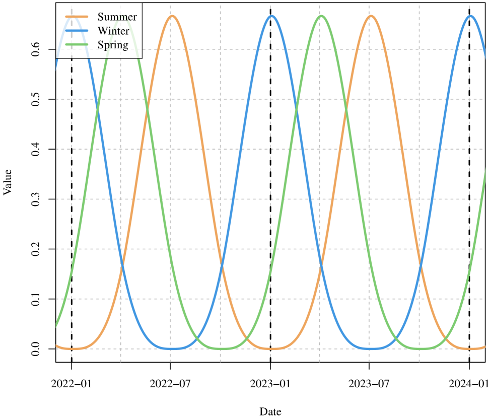
Figure 15: Annual periodic splines used for modeling the annual seasonal component of the power price.

Horizon	1				90				180				360
Model	No fuels		Fuels		No fuels		Fuels		No fuels		Fuels		No fuels		Fuels
Diff	No	Yes	No	Yes	No	Yes	No	Yes	No	Yes	No	Yes	No	Yes	No	Yes
2018	6.69	5.18	4.97	5.18	17.44	17.21	14.64	17.15	19.59	21.15	18.79	21.06	21.33	21.02	21.34	21.00
2019	5.77	5.76	5.42	5.74	9.02	14.83	11.34	14.74	9.12	17.24	13.18	17.20	10.71	17.25	10.76	17.25
2020	5.59	5.63	5.08	5.61	11.69	16.56	16.30	16.47	12.51	19.01	16.20	18.98	11.54	16.51	12.39	16.52
2021	17.70	17.08	16.54	17.12	48.30	45.21	44.27	45.16	61.70	56.31	65.62	56.28	62.99	68.59	69.13	68.60
2022	39.98	39.29	38.95	39.32	162.16	157.35	124.32	158.00	148.88	138.69	129.13	138.78	210.44	157.72	202.26	157.72
2023	17.90	17.34	17.18	17.26	52.20	63.81	92.29	63.79	183.78	122.51	206.57	122.29	382.90	152.13	373.55	152.26
2024	17.37	20.56	19.57	20.50	51.37	43.72	70.59	43.67	65.92	46.28	134.58	46.08	108.63	57.20	156.44	57.16

Table 11: Yearly MAE (EUR/MWh) out-of-sample showing effect of differencing with and without fuels as regressors for selected forecasting horizons.

	1	7	14	30	60	90	120	150	180	210	240	270	300	330	360
No constr	$16.60$	$29.57$	$34.58$	$45.79$	$49.25$	$61.48$	$65.82$	$76.08$	$95.87$	$117.70$	$128.18$	$127.45$	$160.40$	$175.30$	$163.87$
Constr	16.58	29.47	33.85	$41.98$	$47.26$	$57.16$	$64.53$	$71.10$	$84.07$	$91.07$	$105.95$	$116.76$	$125.44$	$130.59$	$130.45$
Constr diff	$17.82$	$35.74$	$39.93$	$46.62$	$52.51$	$57.02$	$58.02$	$62.13$	$66.70$	$66.68$	68.86	$70.79$	$74.93$	$75.93$	$78.41$
Portfolio	$16.69$	$30.93$	$37.36$	$48.17$	$55.76$	$68.45$	$75.96$	$80.28$	$89.19$	$96.36$	$108.23$	$117.24$	$131.88$	$134.63$	$137.72$
Short-term	$20.29$	$32.08$	$36.47$	$43.10$	$48.07$	$56.58$	$64.25$	$74.31$	$85.83$	$93.29$	$104.45$	$114.91$	$126.28$	$135.53$	$136.15$
Current	$20.29$	$32.23$	$35.61$	40.31	44.70	49.12	52.62	56.02	61.02	65.55	$69.00$	67.83	72.38	73.58	75.05

Table 12: MAE (EUR/MWh) for the evaluation period April/2018-April/2023 for all considered models and forecasting horizons over all 24 hours.

Year	Model/Horizon	1	7	14	30	60	90	120	150	180	210	240	270	300	330	360
2018	No constr	$4.73$	$10.04$	$10.13$	$11.41$	$14.64$	$17.88$	$24.26$	$21.52$	$25.69$	$25.70$	$22.14$	$21.13$	$23.54$	$22.23$	$21.34$
	Constr	$4.72$	9.88	9.97	10.90	12.82	14.68	$16.33$	17.50	$18.79$	$19.24$	$19.55$	$19.70$	$20.08$	$19.66$	19.41
	Constr diff	$5.02$	$12.28$	$12.69$	$13.14$	$15.81$	$17.18$	16.12	$19.25$	$21.10$	$20.98$	$20.72$	$20.90$	$20.69$	$20.35$	$21.01$
	Portfolio	4.65	$10.05$	$10.48$	$12.55$	$15.88$	$17.77$	$17.01$	$17.63$	18.31	18.96	$19.59$	19.61	19.71	19.40	$19.41$
	Short-term	$8.07$	$10.22$	$10.45$	$11.45$	$13.34$	$15.46$	$17.41$	$18.96$	$19.95$	$20.65$	$21.18$	$21.71$	$21.72$	$21.68$	$21.50$
	Current	$8.07$	$10.37$	$10.83$	$11.99$	$13.67$	$14.81$	$16.66$	$17.96$	$18.44$	$19.05$	19.51	$19.81$	$19.92$	$20.17$	$20.20$
2019	No constr	4.94	$7.83$	$8.19$	8.48	$8.86$	9.82	$12.73$	$22.25$	$18.80$	$19.58$	$24.22$	$25.51$	$27.26$	$32.86$	$21.46$
	Constr	$4.94$	7.80	8.18	$8.49$	8.68	$9.90$	$11.36$	$13.29$	$14.01$	$13.18$	$14.67$	$13.42$	10.90	10.03	10.03
	Constr diff	$5.83$	$11.69$	$12.17$	$13.41$	$14.23$	$14.83$	$14.75$	$17.08$	$17.22$	$17.23$	$18.10$	$18.79$	$18.12$	$16.90$	$17.37$
	Portfolio	$5.16$	$8.27$	$9.11$	$10.13$	$10.60$	$13.78$	$14.45$	$16.81$	$17.17$	$22.70$	$19.48$	$14.42$	$12.05$	$10.73$	$10.48$
	Short-term	$7.41$	$8.92$	$9.14$	$9.57$	$9.78$	$11.02$	$12.78$	$14.33$	$14.12$	$14.16$	$14.97$	$14.13$	$12.13$	$10.92$	$11.57$
	Current	$7.41$	$8.90$	$9.17$	$9.46$	$9.93$	$10.24$	10.55	11.30	11.53	11.13	11.18	11.28	$11.59$	$11.71$	$11.86$
2020	No constr	$4.76$	$8.24$	$8.67$	$9.46$	11.04	$13.22$	$15.31$	$14.84$	$15.25$	$15.78$	$14.41$	$15.29$	$16.61$	$25.78$	$31.44$
	Constr	4.72	8.22	8.65	9.41	$11.05$	$13.14$	$14.83$	$13.98$	$13.63$	$12.97$	$12.76$	$12.74$	$12.29$	11.95	10.63
	Constr diff	$5.60$	$11.61$	$12.21$	$13.08$	$15.23$	$16.51$	$16.37$	$18.46$	$18.99$	$18.58$	$17.78$	$18.00$	$16.26$	$14.33$	$16.57$
	Portfolio	$4.97$	$9.31$	$10.01$	$11.27$	$12.93$	$13.66$	$14.51$	13.49	13.37	12.73	12.59	12.35	12.20	$12.35$	$11.74$
	Short-term	$7.70$	$9.25$	$9.62$	$10.43$	$12.26$	$14.25$	$14.33$	$14.94$	$14.94$	$14.06$	$13.22$	$12.75$	$12.90$	$13.25$	$12.06$
	Current	$7.70$	$9.25$	$9.66$	$10.46$	$11.27$	12.25	13.41	$13.91$	$14.78$	$14.97$	$15.04$	$15.15$	$14.96$	$15.04$	$15.51$
2021	No constr	$16.22$	$28.20$	$30.48$	$32.28$	31.96	39.57	48.74	$60.33$	$72.18$	$75.23$	$74.51$	$74.60$	$71.20$	$69.36$	$68.99$
	Constr	$16.36$	$27.65$	$29.95$	$31.19$	$33.16$	$42.14$	$51.62$	$61.20$	$66.39$	$67.38$	$67.46$	$67.15$	$67.45$	$67.55$	$67.37$
	Constr diff	$16.98$	$32.83$	$34.92$	$36.52$	$39.76$	$45.15$	$50.32$	52.70	$56.29$	58.32	$61.43$	$64.00$	$65.01$	$66.79$	$68.59$
	Portfolio	16.15	27.42	28.61	30.15	$32.90$	$42.68$	$53.05$	$63.40$	$67.14$	$68.08$	$68.11$	$67.45$	$66.70$	65.01	63.57
	Short-term	$21.48$	$29.55$	$31.70$	$33.32$	$35.73$	$44.75$	$53.37$	$63.21$	$69.46$	$71.48$	$71.57$	$70.62$	$70.12$	$70.47$	$71.06$
	Current	$21.48$	$29.72$	$31.83$	$34.23$	$37.68$	$44.95$	$49.80$	$53.29$	56.22	$58.64$	61.27	63.12	64.75	$65.50$	$65.74$
2022	No constr	37.44	$82.44$	$97.79$	$117.30$	$120.99$	116.41	113.36	$137.33$	$121.29$	$142.84$	$179.34$	$215.60$	$271.51$	$263.14$	$212.66$
	Constr	$37.74$	81.63	95.62	113.01	119.00	$123.90$	$130.58$	$125.58$	$130.98$	$147.92$	$164.62$	$175.20$	$174.44$	$178.77$	$186.07$
	Constr diff	$40.10$	$90.49$	$106.58$	$134.03$	$153.36$	$157.84$	$144.46$	$131.23$	$138.77$	$131.28$	138.56	140.31	155.86	159.81	157.66
	Portfolio	$38.34$	$88.18$	$110.75$	$127.79$	$141.35$	$129.52$	$116.16$	$117.60$	118.35	126.88	$153.43$	$187.27$	$195.22$	$180.87$	$186.14$
	Short-term	$44.73$	$82.13$	$95.67$	$113.21$	$119.72$	$121.47$	$127.21$	$122.89$	$128.10$	$146.66$	$163.11$	$172.07$	$174.50$	$180.07$	$187.58$
	Current	$44.73$	$82.79$	$96.06$	$115.17$	$133.20$	$137.76$	$128.40$	115.33	$124.45$	$137.01$	$145.72$	$151.53$	$163.32$	$167.77$	$171.54$
2023	No constr	$17.30$	$30.01$	$38.96$	$72.41$	$81.51$	$125.56$	$146.34$	$172.87$	$200.01$	$209.10$	$229.10$	$263.12$	$380.77$	$480.44$	$400.17$
	Constr	16.79	29.45	$37.74$	$60.85$	$71.33$	$96.95$	$122.74$	$164.81$	$199.76$	$230.29$	$292.09$	$347.92$	$397.83$	$410.47$	$373.17$
	Constr diff	$17.32$	$38.25$	$41.13$	$52.90$	$56.28$	$63.95$	75.90	104.71	$122.65$	129.22	136.95	$139.80$	$151.33$	$151.55$	$153.15$
	Portfolio	$16.89$	$30.92$	$42.70$	$80.99$	$101.07$	$149.63$	$187.75$	$204.77$	$219.88$	$236.93$	$271.44$	$300.74$	$363.21$	$365.01$	$356.07$
	Short-term	$22.26$	$33.76$	$41.96$	$58.97$	$69.09$	$92.73$	$117.07$	$162.03$	$199.25$	$233.19$	$294.07$	$347.99$	$409.92$	$446.69$	$405.77$
	Current	$22.26$	$32.90$	35.40	40.36	45.85	57.81	$79.77$	$104.91$	120.33	$133.87$	$146.65$	128.64	137.63	137.64	136.31
2024	No constr	$18.92$	20.72	$23.41$	$34.80$	$41.15$	$64.27$	$58.42$	$48.83$	$147.69$	$243.65$	$247.52$	$170.56$	$195.03$	$180.22$	$248.47$
	Constr	$18.95$	$22.07$	$22.98$	$28.96$	$40.33$	$56.92$	$56.02$	$47.72$	$79.66$	$74.69$	$84.12$	$84.14$	$89.70$	$104.79$	$135.41$
	Constr diff	$21.08$	$29.56$	$32.57$	$29.75$	$36.17$	$43.86$	$46.31$	$48.61$	$46.29$	$45.46$	$40.35$	$43.82$	$43.00$	$46.21$	$57.11$
	Portfolio	$18.61$	$21.47$	22.97	28.69	$35.68$	$61.43$	$69.84$	$65.61$	$99.24$	$110.82$	$124.35$	$121.23$	$141.91$	$173.80$	$198.29$
	Short-term	18.18	$28.84$	$30.70$	$33.08$	$41.83$	$55.26$	$60.74$	$68.47$	$89.11$	$80.21$	$69.76$	$71.88$	$78.10$	$91.77$	$128.84$
	Current	$18.18$	$29.83$	$31.52$	$32.18$	30.27	31.70	33.78	37.40	38.78	37.70	34.14	37.24	42.04	43.83	49.34

Table 13: Yearly MAE (EUR/MWh) for the evaluation period April/2018-April/2023 for all considered models and forecasting horizons over all 24 hours.

References

- Ziel and Steinert [2018] F. Ziel and R. Steinert. Probabilistic mid-and long-term electricity price forecasting. Renewable and Sustainable Energy Reviews, 94:251–266, 2018.
- Abroun et al. [2024] M. Abroun, A. Jahangiri, A. G. Shamim, and H. Heidari. Predicting long-term electricity prices using modified support vector regression method. Electrical Engineering, pages 1–12, 2024.