Multiple Quantum Harmonic Oscillators in the Tsallis statistics

Abstract

We studied multiple quantum harmonic oscillators in the Tsallis statistics of entropic parameter $q>1$, separately applying the unnormalized $q$-expectation value and the normalized $q$-expectation value (escort average). We obtained the expressions of the energy and the Tsallis entropy, using the Barnes zeta function. For the same oscillators, we obtained the expressions of the energy, the Tsallis entropy, the average level of the oscillators, and the heat capacity. Numerically, we calculated the energy, the Tsallis entropy, and the heat capacity for various $N$ and $q$, using the expansion of the Barnes zeta function with the Hurwitz zeta function, where $N$ is the number of independent oscillators. It was shown from the requirement for the Barnes zeta function that the quantity $N(q-1)$ is less than one. In the Tsallis statistics with the unnormalized $q$-expectation value, the energy, the Tsallis entropy, and the heat capacity are $N$-dependent and $q$-dependent. The $N$-dependences and the $q$-dependences of these quantities at low temperature are different from those at high temperature. The heat capacity is the Schottky-type. These quantities are affected by zero point energy. In the Tsallis statistics with the normalized $q$-expectation value, the $N$-dependences and the $q$-dependences of the energy per oscillator and those of the heat capacity are quite weak, when the equilibrium temperature, which is often called the physical temperature, is adopted. The $N$-dependence and the $q$-dependence of the Tsallis entropy are clearly seen.

1 Introduction

Extension of the Boltzmann-Gibbs statistics has been attempted, and one of extended statistics is the Tsallis statistics Tsallis:Book which is widely used to describe various phenomena. The Tsallis statistics is one parameter extension of the Boltzmann-Gibbs statistics, and the introduced parameter $q$ is called entropic parameter. This statistics is based on the Tsallis entropy and the expectation value. The different expectation values are applied separately in this statistics: the unnormalized $q$-expectation value or the normalized $q$-expectation value (escort average) is employed Tsallis:PhysicaA:1998 . The normalized $q$-expectation value has an appropriate property: the normalized $q$-expectation value of unit operator $\hat{1}$ is one. The Tsallis statistics with the unnormalized $q$-expectation value is often called the Tsallis-2 statistics, and the statistics with the normalized $q$-expectation value is often called the Tsallis-3 statistics.

The system of harmonic oscillators is basic, as the system of free particles is. It is significant to calculate quantities for the systems in the Tsallis statistics. The number of constituents is restricted in the Tsallis statistics Abe-PLA:2001 ; Lenzi:PLA:2001 ; Ishihara:EPJB:2022 ; Ishihara:EPJB:2023 , while that is not restricted in the Boltzmann-Gibbs statistics. Such differences between the Tsallis statistics and the Boltzmann-Gibbs statistics may be clearly seen in simple systems. Therefore, it is worth to study the system of independent constituents in the Tsallis statistics.

Heat capacity often appears in the study of the Tsallis statistics. The Tsallis distribution appears in the system of the constant heat capacity Wada2003 . The temperature fluctuation generates the $q$-exponential type distribution and is related to the heat capacity Wilk:EPJA40:2009 . The condition between the entropic parameter and the heat capacity was also shown Ishihara:EPJP:03:2023 . It is worth to study the heat capacity, because the heat capacity in the Tsallis statistics plays important roles.

It is not easy to calculate the quantities without approximations even for independent oscillators in the Tsallis statistics, because the calculation for multiple oscillators cannot be decomposed into the calculation for a single oscillator. This comes from the property of $q$-exponential function $\exp_{q}(x)$: generally, the function $\exp_{q}(x+y)$ is not equal to $\exp_{q}(x)\exp_{q}(y)$. Therefore, some approximations such as factorization approximation Buyukkilic:PLA:1995 ; Ubriaco:PRE:2000 ; Lenzi:PLA:2001 , high temperature approximationIshihara:EPJB:2022 , or both are applied to proceed with calculations. The validity of approximations was studied in the classical independent system of harmonic oscillators Lenzi:PLA:2001 . The calculations without such approximations in quantum systems are required to avoid the effects of approximations.

The Barnes zeta function Ruijsenaars:2000 ; Kirsten:2010 often appears in the calculations in the Tsallis statistics Ishihara:EPJB:2022 ; Ishihara:EPJB:2023 ; Oprisan . The value of a quantity can be estimated when the value of the Barnes zeta function is estimated. The Barnes zeta function can be expanded with the Hurwitz zeta function Elizalde1989 , and the expansion is simplified in a certain case. The representations of these zeta functions are useful.

The purpose of this paper is to study the system of oscillators in the Tsallis statistics. The unnormalized $q$-expectation value and the normalized $q$-expectation value are employed separately. We calculate some quantities for independent oscillators of the total energy ${\displaystyle E=\sum_{j=1}^{N}(a_{j}n_{j}+b_{j})}$, where $N$ is the number of constituents. The system of quantum harmonic oscillators has such energy. Especially, we focus on the system of the oscillators with same frequency: $a_{1}=a_{2}=\cdots=a_{N}$. We represent the quantities without approximation, using the Barnes zeta function. We calculate numerically the energy, the Tsallis entropy, and the heat capacity, using the expansion of the Barnes zeta function with the Hurwitz zeta function.

We found the following facts. In the Tsallis statistics of entropic parameter $q>1$ with the unnormalized $q$-expectation value, the energy, the Tsallis entropy, and the heat capacity are $N$-dependent and $q$-dependent: the $N$-dependences and $q$-dependences of these quantities at low temperature are different from those at high temperature. The heat capacity is the Schottky-type: the heat capacity increases with the temperature, reaches the peak, and decreases after that. These quantities are affected by zero point energy. In the Tsallis statistics of entropic parameter $q>1$ with the normalized $q$-expectation value, the $N$-dependence and the $q$-dependence of the energy per oscillator and those of the heat capacity are quite weak, when the equilibrium temperature Imdiker:EPJC:2023 ; Ishihara:EPJP:2023:1 ; Ishihara:EPJP:2023:2 , which is often called the physical temperature Abe-PLA:2001 ; Ishihara:EPJP:2023:1 ; Ishihara:EPJP:2023:2 ; Kalyana:2000 ; S.Abe:physicaA:2001 ; Aragao:2003 ; Ruthotto:2003 ; Toral:2003 ; Suyari:2006 ; Ishihara:phi4 ; Ishihara:free-field , is adopted. The equilibrium temperature dependence of the heat capacity in this statistics is similar to that in the Boltzmann-Gibbs statistics. In contrast, the Tsallis entropy are $N$-dependent and $q$-dependent.

This paper is organized as follows. In Sec. 2, we give a brief review of the Tsallis statistics. The unnormalized $q$-expectation value and the normalized $q$-expectation value are introduced. We also give the expansion of the Barnes zeta function with the Hurwitz zeta function. In Sec. 3 and Sec. 4, we attempt to calculate the energy, the Tsallis entropy, and the heat capacity for multiple quantum harmonic oscillators in the Tsallis statistics. The unnormalized $q$-expectation value is employed in Sec. 3 and the normalized $q$-expectation value is employed in Sec. 4. Last section is assigned for discussions and conclusions. In A, we give the brief derivation of the expansion of the Barnes zeta function with the Hurwitz zeta function according to the strategy given in the previous study. We also give another type of the derivation of the expansion.

2 Tsallis statistics and Barnes zeta function

2.1 Brief review of the Tsallis statistics

The Tsallis statistics is based on the Tsallis entropy and the expectation value. The Tsallis entropy of entropic parameter $q$ is defined by

$$S_{\mathrm{T}q}=-\mathrm{Tr}\left[\hat{\rho}^{q}\ln_{q}\hat{\rho}\right]=-\mathrm{Tr}\left[\frac{\hat{\rho}-\hat{\rho}^{q}}{1-q}\right],$$ (1)

where $\hat{\rho}$ is the density operator and $\ln_{q}(x)$ is the $q$-logarithmic function.

A candidate of the expectation value for a quantity $\hat{A}$ is given by

$$\langle\hat{A}\rangle_{q}^{(2)}=\mathrm{Tr}\left[\hat{\rho}^{q}\hat{A}\right].$$ (2)

This is called the unnormalized $q$-expectation value. The Tsallis statistics with the unnormalized $q$-expectation value is often called the Tsallis-2 statistics. The density operator $\hat{\rho}^{(2)}$ in the Tsallis-2 statistics is given by applying the maximum entropy principle. The following functional $I^{(2)}$ is extremized with the energy constraint $\langle\hat{H}\rangle_{q}^{(2)}=U$:

$$I^{(2)}=S_{\mathrm{T}q}-\alpha^{(2)}(\mathrm{Tr}\left[\hat{\rho}\right]-1)-\beta^{(2)}(\langle\hat{H}\rangle_{q}^{(2)}-U),$$ (3)

where $\alpha^{(2)}$ and $\beta^{(2)}$ are the Lagrange multipliers and $\mathrm{Tr}$ indicates the trace. The density operator $\hat{\rho}^{(2)}$ is given by

$$\hat{\rho}^{(2)}=\frac{1}{Z^{(2)}}\exp_{q}(-\beta^{(2)}\hat{H}),$$ (4a)

$$Z^{(2)}=\mathrm{Tr}\left[\exp_{q}(-\beta^{(2)}\hat{H})\right],$$ (4b)

where $\exp_{q}(x)$ is the $q$-exponential function.

Another candidate of the expectation value for a quantity $\hat{A}$ is given by

$$\langle\hat{A}\rangle^{\mathrm{(3)}}_{q}=\frac{\mathrm{Tr}\left[\hat{\rho}^{q}\hat{A}\right]}{\mathrm{Tr}\left[\hat{\rho}^{q}\right]}.$$ (5)

This is called the normalized $q$-expectation value or the escort average. The Tsallis statistics with the normalized $q$-expectation value is often called the Tsallis-3 statistics. The density operator $\hat{\rho}^{(3)}$ in the Tsallis-3 statistics is also given by applying the maximum entropy principle. The following functional $I^{(3)}$ is extremized with the energy constraint $\langle\hat{H}\rangle^{\mathrm{(3)}}_{q}=U$:

$$I^{(3)}=S_{\mathrm{T}q}-\alpha^{(3)}(\mathrm{Tr}\left[\hat{\rho}\right]-1)-\beta^{(3)}(\langle\hat{H}\rangle^{\mathrm{(3)}}_{q}-U),$$ (6)

where $\alpha^{(3)}$ and $\beta^{(3)}$ are the Lagrange multipliers. The density operator $\hat{\rho}^{(3)}$ is given by

$$\hat{\rho}^{(3)}=\frac{1}{Z^{(3)}}\exp_{q}\left(-\frac{\beta^{(3)}}{c_{q}}(\hat{H}-U)\right),$$ (7a)

$$Z^{(3)}=\mathrm{Tr}\left[\exp_{q}\left(-\frac{\beta^{(3)}}{c_{q}}(\hat{H}-U)\right)\right],$$ (7b)

$$c_{q}\equiv\mathrm{Tr}\left[(\hat{\rho}^{(3)})^{q}\right].$$ (7c)

There is the following relation between $Z^{(3)}$ and $c_{q}$:

$$c_{q}=\left(Z^{(3)}\right)^{1-q}.$$ (8)

We introduce the notation $\beta_{\mathrm{ph}}^{(3)}$ which is the inverse of the equilibrium temperature. The equilibrium temperature is often called the physical temperature. The quantity $\beta_{\mathrm{ph}}^{(3)}$ is defined as

$$\beta_{\mathrm{ph}}^{(3)}=\beta^{(3)}/c_{q}.$$ (9)

With these relations, we calculate some quantities for multiple quantum harmonic oscillators in the Tsallis statistics, applying separately the unnormalized $q$-expectation value and the normalized $q$-expectation value.

2.2 The expansion of the Barnes zeta function with the Hurwitz zeta function

We use the following expressions for the Hurwitz zeta function $\zeta_{\mathrm{H}}$ and the Barnes zeta function $\zeta_{\mathrm{B}}$. The Hurwitz zeta function $\zeta_{\mathrm{H}}(s,a)$ Shpot2016 is given by

$$\zeta_{\mathrm{H}}(s,a)=\sum_{n=0}^{\infty}\frac{1}{(n+a)^{s}}.$$ (10)

The Barnes zeta function $\zeta_{\mathrm{B}}(s,a|a_{1},\cdots,a_{N})$ is given by

$$\zeta_{\mathrm{B}}(s,a|a_{1},\cdots,a_{N})=\sum_{n_{1}=0,n_{2}=0,\cdots,n_{N}=0}^{\infty}\frac{1}{(a+n_{1}a_{1}+\cdots+n_{N}a_{N})^{s}},$$ (11)

where $a$, $a_{1}$, $\cdots$, $a_{N}$ are positive and $s$ is larger than $N$ Ruijsenaars:2000 . The Barnes zeta function is a generalization of the Hurwitz zeta function. We often write $\zeta_{\mathrm{B}}(s,a|a_{1},\cdots,a_{N})$ as $\zeta_{\mathrm{B}}(s,a|\vec{a}_{N})$, where $\vec{a}_{N}$ represents the set $(a_{1},a_{2},\cdots,a_{N})$. We also use the notation $\vec{1}_{N}$ to represent the set $(a_{1}=1,a_{2}=1,\cdots,a_{N}=1)$. Therefore, the expression $\zeta_{\mathrm{B}}(s,a|\vec{1}_{N})$ indicates

$$\zeta_{\mathrm{B}}(s,a|\vec{1}_{N})=\sum_{n_{1}=0,n_{2}=0,\cdots,n_{N}=0}^{\infty}\frac{1}{(a+n_{1}+\cdots+n_{N})^{s}}.$$ (12)

As given in the appendix, the Barnes zeta function can be represented with the Hurwitz zeta function. The Barnes zeta function for $a_{1}=a_{2}=\cdots=a_{N}$ is given by

$$\left.\zeta_{B}(s,a|a_{1},\cdots,a_{N})\right|_{a_{1}=a_{2}=\cdots=a_{N}} =\frac{1}{(a_{1})^{s}}\left[\zeta_{H}(s,d)+\sum_{p=1}^{\infty}\left(\begin{array}[]{c}N+p-2\\ p\end{array}\right)\zeta_{H}(s,d+p)\right],$$ (15)

where $d$ is defined by $d=a/a_{1}$ and $\left(\begin{array}[]{c}m\\ n\end{array}\right)$ is the number of combinations. Equation (15) is used in numerical calculations to obtain the values of the Barnes zeta function.

3 Multiple quantum harmonic oscillators in the Tsallis statistics with the unnormalized $q$-expectation value

3.1 Quantities for multiple quantum harmonic oscillators in the Tsallis statistics with the unnormalized $q$-expectation value

In this section, we calculate the energy, the Tsallis entropy, and the heat capacity for multiple quantum harmonic oscillators in the Tsallis-2 statistics: we employ the Tsallis entropy and the unnormalized $q$-expectation value. We consider the total energy of the multiple quantum harmonic oscillators, and the energy is given by

$$E(\{n\})=\sum_{j=1}^{N}(a_{j}n_{j}+b_{j}),$$ (16)

where $a_{j}$ and $b_{j}$ are the coefficients related to the energy of the oscillator numbered $j$, $N$ is the number of the oscillators, and $\{n\}$ represents the set of the quantum numbers, $n_{1},\cdots,n_{N}$. We introduce $a_{\mathrm{eq}}$ by $a_{\mathrm{eq}}=a_{1}$ when the condition $a_{1}=a_{2}=\cdots=a_{N}$ is satisfied. In the same way, we introduce $b_{\mathrm{eq}}$ by $b_{\mathrm{eq}}=b_{1}$ when the condition $b_{1}=b_{2}=\cdots=b_{N}$ is satisfied.

We attempt to obtain expressions in the Tsallis-2 statistics. For example, the unnormalized $q$-expectation value $O^{(2)}$ of a quantity $O$ is calculated by

$$O^{(2)} =\mathrm{Tr}\left[(\hat{\rho}^{(2)})^{q}\hat{O}\right]=\sum_{\{n\}}\big{(}p^{(2)}(\{n\})\big{)}^{q}O(\{n\}),$$ (17a)

$$p^{(2)} =\frac{1}{Z^{(2)}}\exp_{q}(-\beta^{(2)}E(\{n\})),$$ (17b)

$$Z^{(2)} =\sum_{\{n\}}\exp_{q}(-\beta^{(2)}E(\{n\})),$$ (17c)

where $\hat{\rho}^{(2)}$ is the density operator in the Tsallis-2 statistics, $p^{(2)}(\{n\})$ is the probability for the set $\{n\}$ in the Tsallis-2 statistics, and $\hat{O}$ is the operator corresponding to the quantity $O$. The notation $\displaystyle\sum_{\{n\}}$ represents the appropriate sum related to the set $\{n\}$. For example, the energy $U^{(2)}$ is calculated by

$$U^{(2)}=\sum_{\{n\}}\big{(}p^{(2)}(\{n\})\big{)}^{q}E(\{n\})=\sum_{n_{1}=0,\cdots,n_{N}=0}^{\infty}\big{(}p^{(2)}(\{n\})\big{)}^{q}\Bigg{(}\sum_{j=1}^{N}(a_{j}n_{j}+b_{j})\Bigg{)}.$$ (18)

We obtain the probability $p^{(2)}$, the energy $U^{(2)}$, and the Tsallis entropy $S_{\mathrm{T}}^{(2)}$:

$$p^{(2)}=\frac{\left[\alpha^{(2)}_{N}+\displaystyle\sum_{j=1}^{N}a_{j}n_{j}\right]^{1/(1-q)}}{\zeta_{\mathrm{B}}(1/(q-1),\alpha^{(2)}_{N}|\vec{a}_{N})},$$ (19a)

$$U^{(2)}=\frac{1}{\left[\zeta_{\mathrm{B}}(1/(q-1),\alpha^{(2)}_{N}|\vec{a}_{N})\right]^{q-1}}-\frac{\zeta_{\mathrm{B}}(q/(q-1),\alpha^{(2)}_{N}|\vec{a}_{N})}{\left[\zeta_{\mathrm{B}}(1/(q-1),\alpha^{(2)}_{N}|\vec{a}_{N})\right]^{q}},$$ (19b)

$$S_{\mathrm{T}}^{(2)}=\frac{1}{q-1}\left\{1-\frac{\zeta_{\mathrm{B}}(q/(q-1),\alpha^{(2)}_{N}|\vec{a}_{N})}{\left[\zeta_{\mathrm{B}}(1/(q-1),\alpha^{(2)}_{N}|\vec{a}_{N})\right]^{q}}\right\},$$ (19c)

where $\alpha^{(2)}_{N}$ is given by

$$\alpha^{(2)}_{N}=\frac{1+(q-1)\beta^{(2)}\displaystyle\sum_{j=1}^{N}b_{j}}{(q-1)\beta^{(2)}}.$$ (20)

We now focus on the case of $a_{1}=...=a_{N}$ and $b_{1}=...=b_{N}$. We have the probability $p^{(2)}$, the scaled energy $U^{(2)}/a_{\mathrm{eq}}$, the Tsallis entropy $S_{\mathrm{T}}^{(2)}$, and the average level $\overline{n}^{(2)}$ which is defined by

$$\overline{n}^{(2)}=\frac{1}{N}\sum_{n_{1}=0,\cdots,n_{N}=0}^{\infty}\left(\sum_{j=1}^{N}n_{j}\right)\left(p^{(2)}\right)^{q}.$$ (21)

The heat capacity $C^{(2)}$ is defined by

$$C^{(2)}=\frac{\partial U^{(2)}}{\partial T^{(2)}},$$ (22)

where $T^{(2)}$ equals $1/\beta^{(2)}$. These quantities are given by

$$p^{(2)}=\frac{\left[\gamma^{(2)}_{N}+\displaystyle\sum_{j=1}^{N}n_{j}\right]^{1/(1-q)}}{\zeta_{\mathrm{B}}(1/(q-1),\gamma^{(2)}_{N}|\vec{1}_{N})},$$ (23a)

$$\frac{U^{(2)}}{a_{\mathrm{eq}}}=\frac{1}{\left[\zeta_{\mathrm{B}}(1/(q-1),\gamma^{(2)}_{N}|\vec{1}_{N})\right]^{q-1}}-\frac{t^{(2)}}{(q-1)}\frac{\zeta_{\mathrm{B}}(q/(q-1),\gamma^{(2)}_{N}|\vec{1}_{N})}{\left[\zeta_{\mathrm{B}}(1/(q-1),\gamma^{(2)}_{N}|\vec{1}_{N})\right]^{q}},$$ (23b)

$$S_{\mathrm{T}}^{(2)}=\frac{1}{q-1}\left\{1-\frac{\zeta_{\mathrm{B}}(q/(q-1),\gamma^{(2)}_{N}|\vec{1}_{N})}{\left[\zeta_{\mathrm{B}}(1/(q-1),\gamma^{(2)}_{N}|\vec{1}_{N})\right]^{q}}\right\},$$ (23c)

$$\overline{n}^{(2)}=\frac{1}{N}\left\{\frac{1}{\left[\zeta_{\mathrm{B}}(1/(q-1),\gamma^{(2)}_{N}|\vec{1}_{N})\right]^{q-1}}-\gamma^{(2)}_{N}\frac{\zeta_{\mathrm{B}}(q/(q-1),\gamma^{(2)}_{N}|\vec{1}_{N})}{\left[\zeta_{\mathrm{B}}(1/(q-1),\gamma^{(2)}_{N}|\vec{1}_{N})\right]^{q}}\right\},$$ (23d)

$$C^{(2)}=\frac{qt^{(2)}}{(q-1)^{3}}\frac{1}{\left[\zeta_{\mathrm{B}}(1/(q-1),\gamma^{(2)}_{N}|\vec{1}_{N})\right]^{q+1}}$$ (23e)

$$\qquad\qquad\times\left\{\zeta_{\mathrm{B}}(1/(q-1),\gamma^{(2)}_{N}|\vec{1}_{N})\zeta_{\mathrm{B}}((2q-1)/(q-1),\gamma^{(2)}_{N}|\vec{1}_{N})-\left[\zeta_{\mathrm{B}}(q/(q-1),\gamma^{(2)}_{N}|\vec{1}_{N})\right]^{2}\right\},$$ (23f)

where $t^{(2)}$ and $\gamma^{(2)}_{N}$ are given by

$$t^{(2)}=\frac{1}{a_{\mathrm{eq}}\beta^{(2)}},$$ (24a)

$$\gamma^{(2)}_{N}=\frac{t^{(2)}}{(q-1)}+N\left(\frac{b_{\mathrm{eq}}}{a_{\mathrm{eq}}}\right).$$ (24b)

The scaled temperature $t^{(2)}$ should be positive or equal to zero. Therefore, $b_{\mathrm{eq}}$ should be greater than or equal to zero for a positive $a_{\mathrm{eq}}$ in order that $\gamma^{(2)}_{N}$ is not negative.

We can easily show the following relation:

$$U^{(2)}=N(a_{\mathrm{eq}}\overline{n}^{(2)}+b_{\mathrm{eq}})+(1-q)Nb_{\mathrm{eq}}S_{\mathrm{T}}^{(2)}.$$ (25)

In the Boltzmann-Gibbs limit ($q\rightarrow 1$), we have the natural relation:

$$U^{(2)}=N(a_{\mathrm{eq}}\overline{n}^{(2)}+b_{\mathrm{eq}}).$$ (26)

3.2 Numerical results in the Tsallis statistics with the unnormalized $q$-expectation value

In the Tsallis statistics with the unnormalized $q$-expectation value, we treat the case where $a_{1}$, $a_{2}$, $\cdots$, $a_{N}$ are all equal and $b_{1}$, $b_{2}$, $\cdots$, $b_{N}$ are all equal. We use $a_{\mathrm{eq}}$ and $b_{\mathrm{eq}}$ introduced in Subsec. 3.1. We calculate the scaled energy $U^{(2)}/a_{\mathrm{eq}}$, the Tsallis entropy $S_{\mathrm{T}}^{(2)}$, and the heat capacity $C^{(2)}$ as functions of the scaled temperature $t^{(2)}$ numerically. We choose the value of $q$ to satisfy the inequality $(q-1)N<1$, because the Barnes zeta function requires $1/(q-1)>N$.

First, we calculate the scaled energy numerically. Figure 1(a) shows the scaled energies $U^{(2)}/a_{\mathrm{eq}}$ as functions of $t^{(2)}$ at $q=1.04$ and $b_{\mathrm{eq}}/a_{\mathrm{eq}}=0.0$ for $N=1,5,10,15,$ and $20$. Figure 1(b) shows the scaled energies divided by $N$, $(U^{(2)}/a_{\mathrm{eq}})/N$, as functions of $t^{(2)}$ at $q=1.04$ and $b_{\mathrm{eq}}/a_{\mathrm{eq}}=0.0$ for $N=1,5,10,15,$ and $20$. The energy increases with the scaled temperature. The energy per oscillator decreases with $N$ at high scaled temperature, while the energy per oscillator increases with $N$ at low scaled temperature.

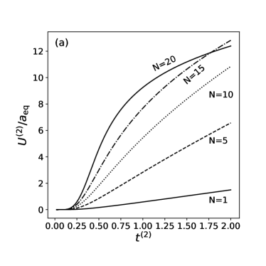
(a) The scaled energy

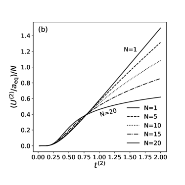
(b) The scaled energy divided by $N$

Figure 1: The scaled energies $U^{(2)}/a_{\mathrm{eq}}$ and the scaled energies divided by $N$, $(U^{(2)}/a_{\mathrm{eq}})/N$, as functions of the scaled temperature $t^{(2)}$ at $q=1.04$ and $b_{\mathrm{eq}}/a_{\mathrm{eq}}=0.0$ for $N=1$, $5$, $10$, $15$, and $20$.

Figure 3 shows the scaled energy $U^{(2)}/a_{\mathrm{eq}}$ at $N=20$ and $b_{\mathrm{eq}}/a_{\mathrm{eq}}=0.0$ for $q=1.01$, $1.02$, $1.03,$ and $1.04$. The energy decreases with $q$ at high scaled temperature, while the energy increases with $q$ at low scaled temperature. Figure 3 shows the scaled energy $U^{(2)}/a_{\mathrm{eq}}$ at $q=1.04$ and $N=20$ for $b_{\mathrm{eq}}/a_{\mathrm{eq}}=0.0$, $0.5$, $1.0$ and $1.5$. The energy decreases and approaches a certain value as the scaled temperature decreases, depending on the value of $b_{\mathrm{eq}}/a_{\mathrm{eq}}$.

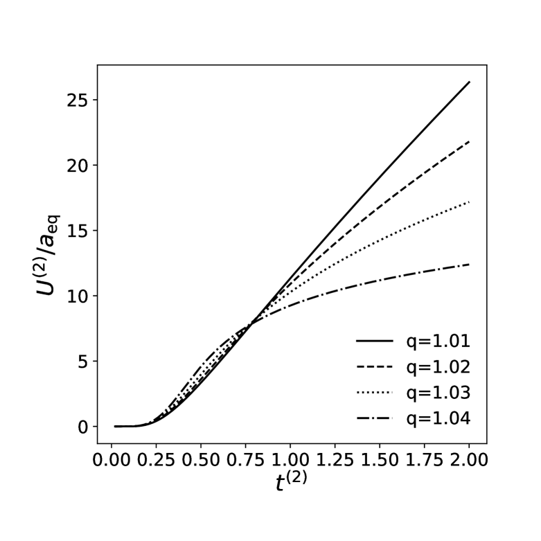
Figure 2: The scaled energies $U^{(2)}/a_{\mathrm{eq}}$ as functions of the scaled temperature $t^{(2)}$ at $N=20$ and $b_{\mathrm{eq}}/a_{\mathrm{eq}}=0.0$ for $q=1.01$, $1.02$, $1.03$, and $1.04$.

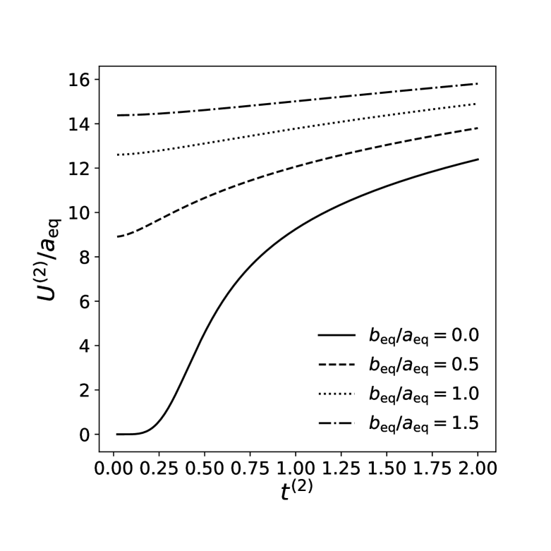
Figure 3: The scaled energies $U^{(2)}/a_{\mathrm{eq}}$ as functions of the scaled temperature $t^{(2)}$ at $q=1.04$ and $N=20$ for $b_{\mathrm{eq}}/a_{\mathrm{eq}}=0.0$, $0.5$, $1.0$, and $1.5$.

Next, we calculate the Tsallis entropy numerically. Figure 4(a) shows the Tsallis entropies $S_{\mathrm{T}}^{(2)}$ as functions of $t^{(2)}$ at $q=1.04$ and $b_{\mathrm{eq}}/a_{\mathrm{eq}}=0.0$ for $N=1$, $5$, $10$, $15$, and $20$. Figure 4(b) shows the Tsallis entropies divided by $N$, $S_{\mathrm{T}}^{(2)}/N$, as functions of $t^{(2)}$ at $q=1.04$ and $b_{\mathrm{eq}}/a_{\mathrm{eq}}=0.0$ for $N=1$, $5$, $10$, $15$, and $20$. The Tsallis entropy per oscillator decreases with $N$ at high scaled temperature, while the Tsallis entropy per oscillator increases with $N$ at low scaled temperature. Figure 6 shows the Tsallis entropies $S_{\mathrm{T}}^{(2)}$ as functions of $t^{(2)}$ at $N=20$ and $b_{\mathrm{eq}}/a_{\mathrm{eq}}=0.0$ for $q=1.01$, $1.02$, $1.03$, and $1.04$. The Tsallis entropy decreases with $q$ at high scaled temperature, while the Tsallis entropy increases with $q$ at low scaled temperature. Figure 6 shows the Tsallis entropies $S_{\mathrm{T}}^{(2)}$ as functions of $t^{(2)}$ at $q=1.04$ and $N=20$ for $b_{\mathrm{eq}}/a_{\mathrm{eq}}=0.0$, $0.5$, $1.0$, and $1.5$. The Tsallis entropies approach non-zero values as $t^{(2)}$ goes to zero, except for $b_{\mathrm{eq}}/a_{\mathrm{eq}}=0.0$. This behavior can be explained from Eq. (24b). The value of $\gamma^{(2)}_{N}$ is positive for $t^{(2)}=0$ and $b_{\mathrm{eq}}/a_{\mathrm{eq}}>0$, while the value of $\gamma^{(2)}_{N}$ is zero for $t^{(2)}=0$ and $b_{\mathrm{eq}}/a_{\mathrm{eq}}=0$. Therefore, the Tsallis entropy $S_{\mathrm{T}}^{(2)}$ at $t^{(2)}=0$ is positive for $b_{\mathrm{eq}}/a_{\mathrm{eq}}>0$.

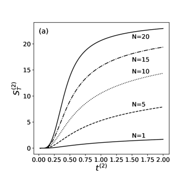
(a) The Tsallis entropy

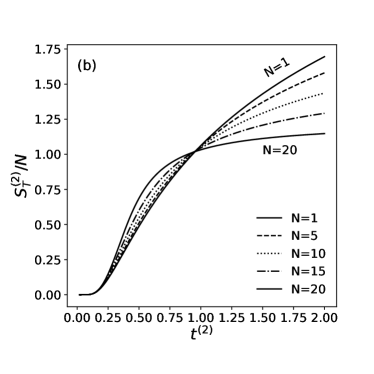
(b) The Tsallis entropy divided by $N$

Figure 4: The Tsallis entropies $S_{\mathrm{T}}^{(2)}$ and the Tsallis entropies divided by $N$, $S_{\mathrm{T}}^{(2)}/N$, as functions of the scaled temperature $t^{(2)}$ at $q=1.04$ and $b_{\mathrm{eq}}/a_{\mathrm{eq}}=0.0$ for $N=1$, $5$, $10$, $15$, and $20$.

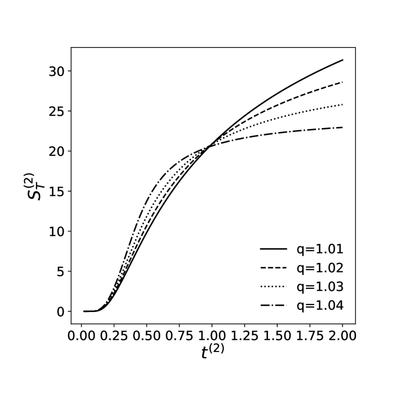
Figure 5: The Tsallis entropies $S_{\mathrm{T}}^{(2)}$ as functions of the scaled temperature $t^{(2)}$ at $N=20$ and $b_{\mathrm{eq}}/a_{\mathrm{eq}}=0.0$ for $q=1.01$, $1.02$, $1.03$, and $1.04$.

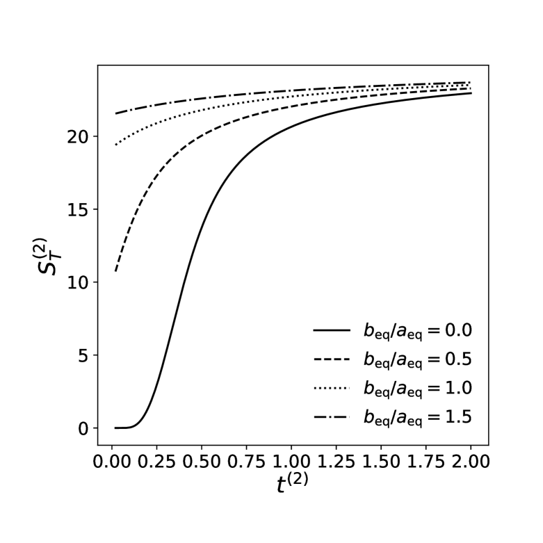
Figure 6: The Tsallis entropies $S_{\mathrm{T}}^{(2)}$ as functions of the scaled temperature $t^{(2)}$ at $q=1.04$ and $N=20$ for $b_{\mathrm{eq}}/a_{\mathrm{eq}}=0.0$, $0.5$, $1.0$, and $1.5$.

Finally, we calculate the heat capacity numerically. Figure 7(a) shows the heat capacities $C^{(2)}$ as functions of $t^{(2)}$ at $q=1.04$ and $b_{\mathrm{eq}}/a_{\mathrm{eq}}=0.0$ for $N=1$, $5$, $10$, $15$, and $20$. The behavior of the heat capacity in the Tsallis-2 statistics is quite different from that in the Boltzmann-Gibbs statistics. As shown in this figure, the heat capacity increases with the scaled temperature, and reaches the maximum, and decreases after that. This behavior reflects the temperature dependence of the energy. Figure 7(b) shows the heat capacities divided by $N$, $C^{(2)}/N$, as functions of $t^{(2)}$ at $q=1.04$ and $b_{\mathrm{eq}}/a_{\mathrm{eq}}=0.0$ for $N=1$, $5$, $10$, $15$, and $20$. The heat capacity per oscillator, $C^{(2)}/N$, decreases with $N$ at high scaled temperature, while the heat capacity per oscillator increases with $N$ at low scaled temperature. Figure 9 shows the heat capacities $C^{(2)}$ as functions of $t^{(2)}$ at $N=20$ and $b_{\mathrm{eq}}/a_{\mathrm{eq}}=0.0$ for $q=1.01$, $1.02$, $1.03$ and $1.04$. The heat capacity decreases as $q$ increases at high scaled temperature, while the heat capacity increases as $q$ increases at low scaled temperature. Figure 9 shows the heat capacities $C^{(2)}$ as functions of $t^{(2)}$ at $q=1.04$ and $N=20$ for $b_{\mathrm{eq}}/a_{\mathrm{eq}}=0.0$, $0.5$, $1.0$, and $1.5$. The heat capacity depends on $b_{\mathrm{eq}}$, because the energy depends on $b_{\mathrm{eq}}$. The variation of the heat capacity is weak for large $b_{\mathrm{eq}}$.

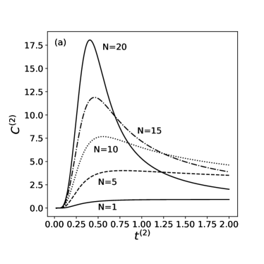
(a) The heat capacities

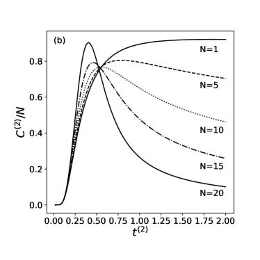
(b) The heat capacities divided by $N$

Figure 7: The heat capacities $C^{(2)}$ and the heat capacities divided by $N$, $C^{(2)}/N$, as functions of the scaled temperature $t^{(2)}$ at $q=1.04$ and $b_{\mathrm{eq}}/a_{\mathrm{eq}}=0.0$ for $N=1$, $5$, $10$, $15$, and $20$.

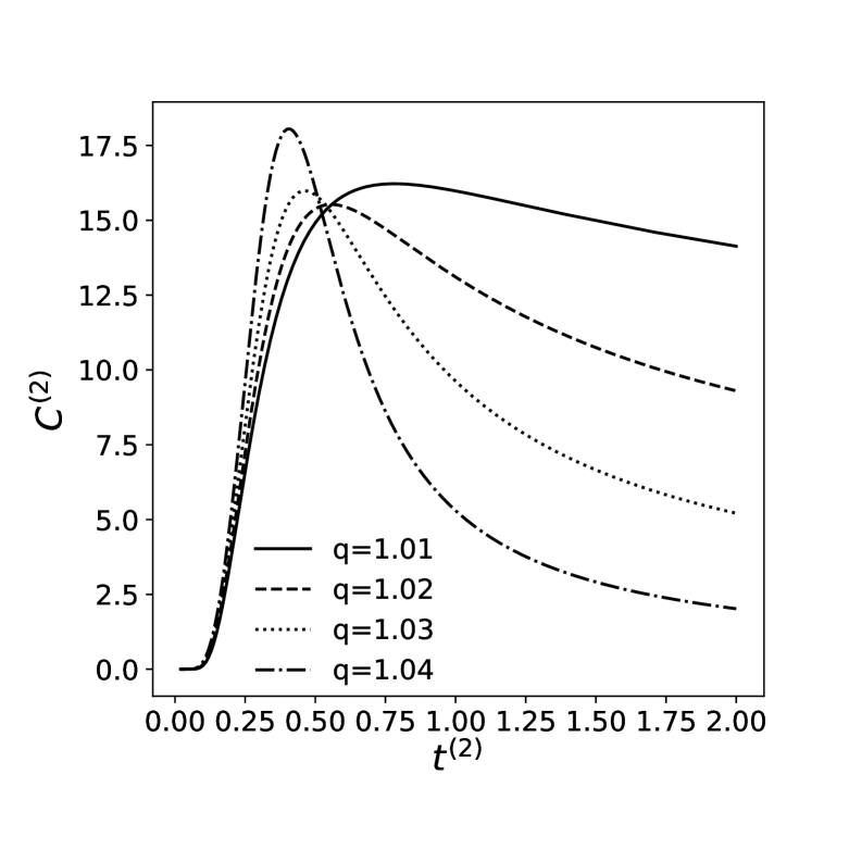
Figure 8: The heat capacities $C^{(2)}$ as functions of the scaled temperature $t^{(2)}$ at $N=20$ and $b_{\mathrm{eq}}/a_{\mathrm{eq}}=0.0$ for $q=1.01$, $1.02$, $1.03$ and $1.04$.

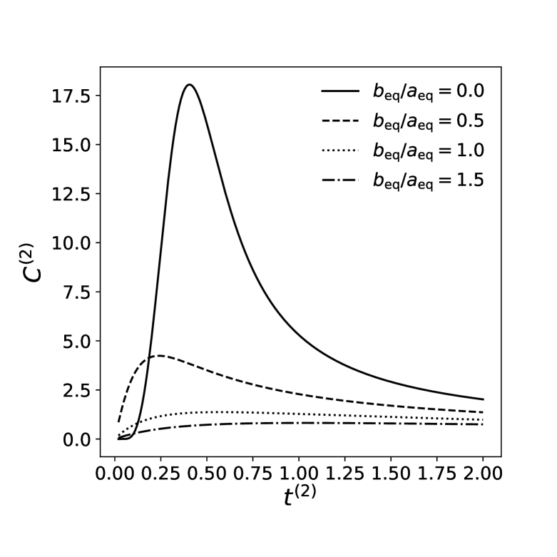
Figure 9: The heat capacities $C^{(2)}$ as functions of the scaled temperature $t^{(2)}$ at $q=1.04$ and $N=20$ for $b_{\mathrm{eq}}/a_{\mathrm{eq}}=0.0$, $0.5$, $1.0$ and $1.5$.

4 Multiple quantum harmonic oscillators in the Tsallis statistics with the normalized $q$-expectation value

4.1 Quantities for multiple quantum harmonic oscillators in the Tsallis statistics with the normalized $q$-expectation value

In this section, we calculate the energy, the Tsallis entropy, and the heat capacity for multiple quantum harmonic oscillators in the Tsallis-3 statistics: we employ the Tsallis entropy and the normalized $q$-expectation value. The probability in the Tsallis-3 statistics is invariant to energy shift. The normalized $q$-expectation value is often called the escort average which satisfies the property $\langle\hat{1}\rangle^{\mathrm{(3)}}_{q}=1$. We consider the energy of the multiple quantum harmonic oscillators whose energy is given by Eq. (16).

We attempt to obtain expressions in the Tsallis-3 statistics. The normalized $q$-expectation value $O^{(3)}$ of a quantity $O$ is calculated by

$$O^{(3)} =\frac{\mathrm{Tr}\left[(\hat{\rho}^{(3)})^{q}\hat{O}\right]}{\mathrm{Tr}\left[(\hat{\rho}^{(3)})^{q}\right]}=\frac{\displaystyle\sum_{\{n\}}\big{(}p^{(3)}(\{n\})\big{)}^{q}O(\{n\})}{\displaystyle\sum_{\{n\}}\big{(}p^{(3)}(\{n\})\big{)}^{q}},$$ (27a)

$$p^{(3)} =\frac{1}{Z^{(3)}}\exp_{q}\Big{(}-\frac{\beta^{(3)}}{c_{q}}\big{(}E(\{n\})-U^{(3)}\big{)}\Big{)},$$ (27b)

$$Z^{(3)} =\sum_{\{n\}}\exp_{q}\Big{(}-\frac{\beta^{(3)}}{c_{q}}\big{(}E(\{n\})-U^{(3)}\big{)}\Big{)},$$ (27c)

where $\hat{\rho}^{(3)}$ is the density operator in the Tsallis-3 statistics and $p^{(3)}(\{n\})$ is the probability for the set $\{n\}$ in the Tsallis-3 statistics. For example, the energy $U^{(3)}$ is calculated by

$$U^{(3)}=\frac{\displaystyle\sum_{\{n\}}\big{(}p^{(3)}(\{n\})\big{)}^{q}E(\{n\})}{\displaystyle\sum_{\{n\}}\big{(}p^{(3)}(\{n\})\big{)}^{q}}=\frac{\displaystyle\sum_{n_{1}=0,\cdots,n_{N}=0}^{\infty}\big{(}p^{(3)}(\{n\})\big{)}^{q}\Bigg{(}\displaystyle\sum_{j=1}^{N}(a_{j}n_{j}+b_{j})\Bigg{)}}{\displaystyle\sum_{n_{1}=0,\cdots,n_{N}=0}^{\infty}\big{(}p^{(3)}(\{n\})\big{)}^{q}}.$$ (28)

Here we define $E_{\mathrm{R}}$ and $U^{(3)}_{\mathrm{R}}$ by

$$E_{\mathrm{R}}=E-\sum_{j=1}^{N}b_{j},$$ (29)

$$U^{(3)}_{\mathrm{R}}=U^{(3)}-\sum_{j=1}^{N}b_{j}.$$ (30)

Evidently, $U^{(3)}_{\mathrm{R}}$ is represented by

$$U^{(3)}_{\mathrm{R}}=\frac{\displaystyle\sum_{\{n\}}(p^{(3)})^{q}E_{\mathrm{R}}}{\displaystyle\sum_{\{n\}}(p^{(3)})^{q}}.$$ (31)

We find the probability $p^{(3)}$, the energy $U^{(3)}_{\mathrm{R}}$, and the Tsallis entropy $S_{\mathrm{T}}^{(3)}$:

$$p^{(3)}=\frac{\Bigg{[}\alpha^{(3)}_{N}+\displaystyle\sum_{j=1}^{N}a_{j}n_{j}\Bigg{]}^{1/(1-q)}}{\zeta_{\mathrm{B}}(1/(q-1),\alpha^{(3)}_{N}|\vec{a}_{N})},$$ (32a)

$$U^{(3)}_{\mathrm{R}}=\frac{\zeta_{\mathrm{B}}(1/(q-1),\alpha^{(3)}_{N}|\vec{a}_{N})}{\zeta_{\mathrm{B}}(q/(q-1),\alpha^{(3)}_{N}|\vec{a}_{N})}-\alpha^{(3)}_{N},$$ (32b)

$$S_{\mathrm{T}}^{(3)}=(q-1)^{-1}\left\{1-\frac{\zeta_{\mathrm{B}}(q/(q-1),\alpha^{(3)}_{N}|\vec{a}_{N})}{\left[\zeta_{\mathrm{B}}(1/(q-1),\alpha^{(3)}_{N}|\vec{a}_{N})\right]^{q}}\right\},$$ (32c)

where $\alpha^{(3)}_{N}$ is given by

$$\alpha^{(3)}_{N}=\frac{1+(1-q)\beta_{\mathrm{ph}}^{(3)}U^{(3)}_{\mathrm{R}}}{(q-1)\beta_{\mathrm{ph}}^{(3)}}.$$ (33)

In the Tsallis-3 statistics, there is the relation $c_{q}=(Z^{(3)})^{1-q}$, where the partition function $Z^{(3)}$ in the present case is given by

$$Z^{(3)}=[(q-1)\beta_{\mathrm{ph}}^{(3)}]^{1/(1-q)}\zeta_{\mathrm{B}}(1/(q-1),\alpha^{(3)}_{N}|\vec{a}_{N}).$$ (34)

This relation $c_{q}=(Z^{(3)})^{1-q}$ gives the self-consistent equation:

$$\zeta_{\mathrm{B}}(q/(q-1),\alpha^{(3)}_{N}|\vec{a}_{N})=(q-1)\beta_{\mathrm{ph}}^{(3)}\zeta_{\mathrm{B}}(1/(q-1),\alpha^{(3)}_{N}|\vec{a}_{N}).$$ (35)

Equation (35) is also derived from Eqs. (32b) and (33). The self-consistent equation, Eq. (35), is consistent with the expression of the energy.

We now focus on the case where $a_{1}$, $a_{2}$, $\cdots$, $a_{N}$ are all equal. It is worth to mention that no condition for $b_{j}$ is imposed, because $p^{(3)}$ does not contain $\displaystyle\sum_{j=1}^{N}b_{j}$. We introduce the following quantity $t_{\mathrm{ph}}^{(3)}$ and $\gamma^{(3)}_{N}$ by

$$t_{\mathrm{ph}}^{(3)}=\frac{1}{a_{\mathrm{eq}}\beta_{\mathrm{ph}}^{(3)}},$$ (36a)

$$\gamma^{(3)}_{N}=\frac{\alpha^{(3)}_{N}}{a_{\mathrm{eq}}}.$$ (36b)

The average level $\overline{n}^{(3)}$ is defined by

$$\overline{n}^{(3)}=\frac{1}{N}\frac{\displaystyle\sum_{n_{1}=0,\cdots,n_{N}=0}^{\infty}\left(\sum_{j=1}^{N}n_{j}\right)\left(p^{(3)}\right)^{q}}{\displaystyle\sum_{n_{1}=0,\cdots,n_{N}=0}^{\infty}\left(p^{(3)}\right)^{q}}.$$ (37)

The heat capacity $C_{\mathrm{ph}}^{(3)}$ is defined by

$$C_{\mathrm{ph}}^{(3)}=\frac{\partial U^{(3)}}{\partial T_{\mathrm{ph}}},$$ (38)

where $T_{\mathrm{ph}}$ is the equilibrium temperature (the physical temperature): $T_{\mathrm{ph}}$ is given by $1/\beta_{\mathrm{ph}}^{(3)}$.

The probability $p^{(3)}$, the scaled energy $U^{(3)}_{\mathrm{R}}/a_{\mathrm{eq}}$, the Tsallis entropy $S_{\mathrm{T}}^{(3)}$, the average level $\overline{n}^{(3)}$, and the heat capacity $C_{\mathrm{ph}}^{(3)}$ are represented by

$$p^{(3)}=\frac{\Bigg{[}\gamma^{(3)}_{N}+\displaystyle\sum_{j=1}^{N}n_{j}\Bigg{]}^{1/(1-q)}}{\zeta_{\mathrm{B}}(1/(q-1),\gamma^{(3)}_{N}|\vec{1}_{N})},$$ (39a)

$$\frac{U^{(3)}_{\mathrm{R}}}{a_{\mathrm{eq}}}=\frac{\zeta_{\mathrm{B}}(1/(q-1),\gamma^{(3)}_{N}|\vec{1}_{N})}{\zeta_{\mathrm{B}}(q/(q-1),\gamma^{(3)}_{N}|\vec{1}_{N})}-\gamma^{(3)}_{N},$$ (39b)

$$S_{\mathrm{T}}^{(3)}=\frac{1}{(q-1)}\left\{1-\frac{\zeta_{\mathrm{B}}(q/(q-1),\gamma^{(3)}_{N}|\vec{1}_{N})}{\Bigg{[}\zeta_{\mathrm{B}}(1/(q-1),\gamma^{(3)}_{N}|\vec{1}_{N})\Bigg{]}^{q}}\right\},$$ (39c)

$$\overline{n}^{(3)}=\frac{1}{N}\left\{\frac{\zeta_{\mathrm{B}}(1/(q-1),\gamma^{(3)}_{N}|\vec{1}_{N})}{\zeta_{\mathrm{B}}(q/(q-1),\gamma^{(3)}_{N}|\vec{1}_{N})}-\gamma^{(3)}_{N}\right\},$$ (39d)

$$C_{\mathrm{ph}}^{(3)}=\frac{\partial U^{(3)}_{\mathrm{R}}}{\partial T_{\mathrm{ph}}}=\frac{\partial(U^{(3)}_{\mathrm{R}}/a_{\mathrm{eq}})}{\partial t_{\mathrm{ph}}^{(3)}}=\frac{1}{(q-1)}\left(\frac{\frac{\partial}{\partial\gamma^{(3)}_{N}}\left(U^{(3)}_{\mathrm{R}}/a_{\mathrm{eq}}\right)}{1+\frac{\partial}{\partial\gamma^{(3)}_{N}}\left(U^{(3)}_{\mathrm{R}}/a_{\mathrm{eq}}\right)}\right)$$

$$\quad\quad=\frac{1}{(q-1)}+\frac{\left[\zeta_{\mathrm{B}}(q/(q-1),\gamma^{(3)}_{N}|\vec{1}_{N})\right]^{2}}{\left[\zeta_{\mathrm{B}}(q/(q-1),\gamma^{(3)}_{N}|\vec{1}_{N})\right]^{2}-q\zeta_{\mathrm{B}}(1/(q-1),\gamma^{(3)}_{N}|\vec{1}_{N})\zeta_{\mathrm{B}}((2q-1)/(q-1),\gamma^{(3)}_{N}|\vec{1}_{N})}.$$ (39e)

The self-consistent equation, Eq. (35), is represented as follows:

$$t_{\mathrm{ph}}^{(3)}\zeta_{\mathrm{B}}(q/(q-1),\gamma^{(3)}_{N}|\vec{1}_{N})=(q-1)\zeta_{\mathrm{B}}(1/(q-1),\gamma^{(3)}_{N}|\vec{1}_{N}).$$ (40)

We can easily find the relation $U^{(3)}_{\mathrm{R}}=Na_{\mathrm{eq}}\overline{n}^{(3)}$. That is

$$U^{(3)}=Na_{\mathrm{eq}}\overline{n}^{(3)}+\sum_{j=1}^{N}b_{j}.$$ (41)

The last term is the zero point energy of the oscillators. The natural relation between the energy and the average level holds in the Tsallis-3 statistics.

4.2 Numerical results in the Tsallis statistics with the normalized $q$-expectation value

In the Tsallis statistics with the normalized $q$-expectation value, we treat the case where $a_{1}$, $a_{2}$, $\cdots$, $a_{N}$ are all equal to $a_{\mathrm{eq}}$. We calculate the scaled energy $U^{(3)}_{\mathrm{R}}/a_{\mathrm{eq}}$, the Tsallis entropy $S_{\mathrm{T}}^{(3)}$, and the heat capacity $C_{\mathrm{ph}}^{(3)}$ as functions of the scaled equilibrium temperature (the scaled physical temperature) $t_{\mathrm{ph}}^{(3)}$ numerically. The value of $q$ is chosen to satisfy the inequality $(q-1)N<1$, as chosen in the previous section.

First, we calculate the scaled energy numerically. Figure 10(a) shows the scaled energies $U^{(3)}_{\mathrm{R}}/a_{\mathrm{eq}}$ as functions of $t_{\mathrm{ph}}^{(3)}$ at $q=1.03$ for $N=1$, $5$, $10$, $15$, and $20$. Figure. 10(b) shows the scaled energies divided by $N$, $(U^{(3)}_{\mathrm{R}}/a_{\mathrm{eq}})/N$, as functions of $t_{\mathrm{ph}}^{(3)}$ at $q=1.03$ for $N=1$, $5$, $10$, $15$, and $20$. The scaled energy $U^{(3)}_{\mathrm{R}}/a_{\mathrm{eq}}$ increases with $t_{\mathrm{ph}}^{(3)}$, and the $N$-dependence of $(U^{(3)}_{\mathrm{R}}/a_{\mathrm{eq}})/N$ is absent. The energy for $N$ oscillators is simply $N$ times the energy for a single oscillator. It is found from Eq. (41) that the $N$-dependence of $\overline{n}^{(3)}$ is absent when the $N$-dependence of $(U^{(3)}_{\mathrm{R}}/a_{\mathrm{eq}})/N$ is absent.

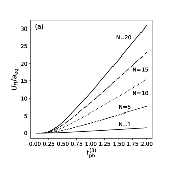
(a) The scaled energy

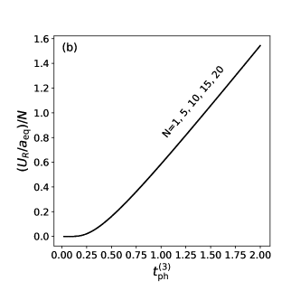
(b) The scaled energy divided by $N$

Figure 10: The scaled energies $U^{(3)}_{\mathrm{R}}/a_{\mathrm{eq}}$ and the scaled energies divided by $N$, $(U^{(3)}_{\mathrm{R}}/a_{\mathrm{eq}})/N$, as functions of the scaled equilibrium temperature (the scaled physical temperature) $t_{\mathrm{ph}}^{(3)}$ at $q=1.03$ for $N=1,5,10,15$, and $20$, where $N$ is the number of oscillators.

Figure 11 shows the scaled energies $U^{(3)}_{\mathrm{R}}/a_{\mathrm{eq}}$ as functions of $t_{\mathrm{ph}}^{(3)}$ at $N=20$ for $q=1.01,1.02,1.03$, and $1.04$. The $q$-dependence of the scaled energy is quite small.

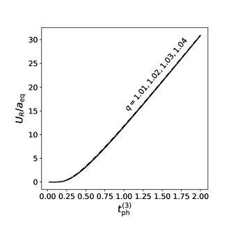
Figure 11: The scaled energies $U^{(3)}_{\mathrm{R}}/a_{\mathrm{eq}}$ as functions of the scaled equilibrium temperature (the scaled physical temperature) $t_{\mathrm{ph}}^{(3)}$ at $N=20$ for $q=1.01,1.02,1.03$, and $1.04$.

Next, we calculate the Tsallis entropy numerically. Figure 12(a) shows the Tsallis entropies $S_{\mathrm{T}}^{(3)}$ as functions of $t_{\mathrm{ph}}^{(3)}$ at $q=1.03$ for $N=1,5,10,15$ and $20$. Figure 12(b) shows the Tsallis entropies divided by $N$, $S_{\mathrm{T}}^{(3)}/N$, as functions of $t_{\mathrm{ph}}^{(3)}$ at $q=1.03$ for $N=1,5,10,15$ and $20$. The Tsallis entropy $S_{\mathrm{T}}^{(3)}$ increases with $t_{\mathrm{ph}}^{(3)}$. The Tsallis entropy per single oscillator decreases with $N$ from Fig. 12(b).

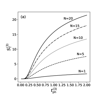
(a) The Tsallis entropy

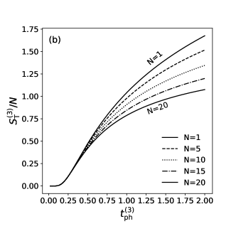
(b) The Tsallis entropy divided by $N$

Figure 12: The Tsallis entropies $S_{\mathrm{T}}^{(3)}$ as functions of the scaled equilibrium temperature (the scaled physical temperature) $t_{\mathrm{ph}}^{(3)}$ at $q=1.03$ for $N=1,5,10,15$, and $20$.

Figure 13 shows the Tsallis entropies $S_{\mathrm{T}}^{(3)}$ as functions of $t_{\mathrm{ph}}^{(3)}$ at $N=20$ for $q=1.01$, $1.02$, $1.03$, and $1.04$. The Tsallis entropy decreases as the entropic parameter $q$ increases.

Figure 13: The Tsallis entropies $S_{\mathrm{T}}^{(3)}$ as functions of the scaled equilibrium temperature (the scaled physical temperature) $t_{\mathrm{ph}}^{(3)}$ at $N=20$ for $q=1.01$, $1.02$, $1.03$, and $1.04$.

Finally, we calculate the heat capacity numerically. Figure 14(a) shows the heat capacities $C_{\mathrm{ph}}^{(3)}$ as functions of $t_{\mathrm{ph}}^{(3)}$ at $q=1.03$ for $N=1$, $5$, $10$, $15$, and $20$. Figure 14(b) shows the heat capacities divided by $N$, $C_{\mathrm{ph}}^{(3)}/N$, as functions of $t_{\mathrm{ph}}^{(3)}$ at $q=1.03$ for $N=1$, $5$, $10$, $15$, and $20$. The difference in the heat capacity divided by $N$ can not be seen in Fig. 14(b). This is an direct result of the temperature dependence of the energy divided by $N$ as shown in Fig. 10(b). Therefore, the heat capacity $C_{\mathrm{ph}}^{(3)}$ for $N$ oscillators is simply $N$ times the heat capacity $C_{\mathrm{ph}}^{(3)}$ for a single oscillator.

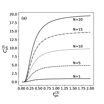
(a) The heat capacity

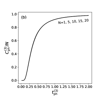
(b) The heat capacity divided by $N$

Figure 14: The heat capacities $C_{\mathrm{ph}}^{(3)}$ and the heat capacities divided by $N$, $C_{\mathrm{ph}}^{(3)}/N$, as functions of the scaled equilibrium temperature (the scaled physical temperature) $t_{\mathrm{ph}}^{(3)}$ at $q=1.03$ for $N=1,5,10,15$, and $20$.

Figure 15 shows the heat capacities $C_{\mathrm{ph}}^{(3)}$ as functions of $t_{\mathrm{ph}}^{(3)}$ at $N=20$ for $q=1.01,1.02,1.03$, and $1.04$. The behavior of the heat capacity reflects the behavior of the energy. Therefore, the $q$-dependence of the heat capacity is quite weak.

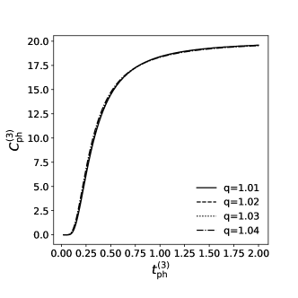
Figure 15: The heat capacities $C_{\mathrm{ph}}^{(3)}$ as functions of the scaled equilibrium temperature (the scaled physical temperature) $t_{\mathrm{ph}}^{(3)}$ at $N=20$ for $q=1.01$, $1.02$, $1.03$, and $1.04$.

5 Discussions and conclusions

We studied the thermodynamic quantities of the system whose energy is represented as $\displaystyle\sum_{j=1}^{N}(a_{j}n_{j}+b_{j})$ in the Tsallis statistics of entropic parameter $q>1$, where $N$ is the number of oscillators. We employed the Tsallis-2 statistics in which the expectation value is the unnormalized $q$-expectation value and the Tsallis-3 statistics in which the expectation value is the normalized $q$-expectation value (the escort average). We obtained the expressions of the energy and the Tsallis entropy. We also obtain the expressions of the energy, the Tsallis entropy, the average level of the oscillators, and the heat capacity for $a_{1}=\cdots=a_{N}$ and $b_{1}=\cdots=b_{N}$ in the Tsallis-2 statistics and for $a_{1}=\cdots=a_{N}$ in the Tsallis-3 statistics. Numerically, we calculated these quantities for $a_{1}=\cdots=a_{N}$ and $b_{1}=\cdots=b_{N}$ in the Tsallis-2 statistics and for $a_{1}=\cdots=a_{N}$ in the Tsallis-3 statistics, using the expansion of the Barnes zeta function with the Hurwitz zeta function.

The quantities are represented with the Barnes zeta function in both the Tsallis-2 and the Tsallis-3 statistics. The Barnes zeta function requires the condition $(q-1)N<1$, where $N$ is the number of the oscillators and $q-1$ is the deviation from the Boltzmann-Gibbs statistics. In the Tsallis-2 statistics, there is the relation among the energy, the average level, and the Tsallis entropy in the present system. The energy depends on the entropic parameter $q$. Therefore, the $q$-dependences of the energy and the heat capacity appear. The zero point energy might play significant roles in the Tsallis-2 statistics, because the zero point energy appears explicitly. In the Tsallis-3 statistics, there is the relation between the energy and the average level in the present system, and the relation is simple. The physical quantities except for the energy are not affected by the zero-point energy, when the equilibrium temperature (the physical temperature) is adopted. The probability is invariant to energy shift and the normalized $q$-expectation value of unit operator $\hat{1}$ is one. In the present case, the self-consistent equation coming from the energy constraint is the same self-consistent equation coming from the normalization condition.

The behaviors were clarified in the Tsallis-2 statistics from the numerical calculations in the system of oscillators with identical energy levels: $a_{1}=a_{2}=\cdots=a_{N}$ and $b_{1}=b_{2}=\cdots=b_{N}$. The physical quantities as functions of the scaled temperature, which is the temperature divided by the difference between adjacent energy levels, depend on $N$ and $q$. The energy, the Tsallis entropy, and the heat capacity were studied. These quantities divided by $N$ increases with $N$ and $q$ at low temperature, while decreases with $N$ and $q$ at high temperature. These indicates that the quantity for $N$ independent oscillators is not $N$ times the quantity for a single oscillator. As shown from the numerical results, the heat capacity has a peak when the system of independent oscillators is described by the temperature $T^{(2)}$ and entropic parameter $q$. The heat capacity resembles the Schottky-type heat capacity.

The behaviors were clarified in the Tsallis-3 statistics from the numerical calculations in the system of oscillators with identical energy difference: $a_{1}=a_{2}=\cdots=a_{N}$. We employed the equilibrium temperature (the physical temperature) to describe the quantities. The $N$-dependence of the energy divided by $N$ cannot be seen. The $N$-dependence of the heat capacity divided by $N$ cannot be also seen, where the heat capacity is defined by the derivative of the energy with respect to the equilibrium temperature. The energy and the heat capacity for $N$-independent oscillators are $N$ times those for a single oscillator. The $q$-dependences of the energy and the heat capacity are quite weak. It seems that finding the difference is difficult. In contrast, the Tsallis entropy divided by $N$ is $N$-dependent and $q$-dependent. The differences can be seen at high equilibrium temperature.

It is not trivial whether the argument of the $q$-exponential, $1+(q-1)\beta_{\mathrm{ph}}^{(3)}(E_{n}-U^{(3)})$, is positive in the Tsallis-3 statistics of $q>1$: the condition of the positivity is not trivial because of the existence of $U^{(3)}$. This condition is rewritten as $1-(q-1)\beta_{\mathrm{ph}}^{(3)}U^{(3)}_{\mathrm{R}}>0$. We found the inequality $(U^{(3)}_{\mathrm{R}}/a_{\mathrm{eq}})/N<t_{\mathrm{ph}}^{(3)}$ from numerical calculations for $a_{1}=\cdots=a_{N}$. This inequality is rewritten as $\beta_{\mathrm{ph}}^{(3)}U^{(3)}_{\mathrm{R}}<N$. With this result, we have the inequality $1-(q-1)\beta_{\mathrm{ph}}^{(3)}U^{(3)}_{\mathrm{R}}>1-(q-1)N$. Therefore, the condition of the positivity is satisfied when $(q-1)N$ is less than one. The condition, $(q-1)N<1$, already appeared in the numerical calculation to choose the value of $q$.

In this paper, we studied the system of $N$-independent oscillators in the Tsallis statistics of $q>1$, using the expansion of the Barnes zeta function with the Hurwitz zeta function. Our results can be applied to the system whose energy is given by $\displaystyle\sum_{j}(a_{j}n_{j}+b_{j})$. I hope that this work is helpful in the future studies related to unconventional statistics.

Funding This research received no specific grant from any funding agency in the public, commercial, or not-for-profit sectors.

Data availability This manuscript has no associated data or the data will not be deposited. [Authors’ comment: This study is theoretical, and the graphs were drawn with the equations given in this paper.].

Conflict of interest The author declares no competing interest.

Appendix A The expansion of the Barnes zeta function with the Hurwitz zeta function

The Hurwitz zeta function $\zeta_{H}(s,a)$ and the Barnes zeta function $\zeta_{B}(s,a|a_{1},\cdots,a_{N})$ are defined by

$$\zeta_{H}(s,a)=\sum_{n=0}^{\infty}\frac{1}{(n+a)^{s}},$$ (42a)

$$\zeta_{B}(s,a|a_{1},\cdots,a_{N})=\sum_{n_{1}=0}^{\infty}\sum_{n_{2}=0}^{\infty}\cdots\sum_{n_{N}=0}^{\infty}\frac{1}{(a+a_{1}n_{1}+a_{2}n_{2}+\cdots+a_{N}n_{N})^{s}}.$$ (42b)

The Barnes zeta function $\zeta_{B}(s,a|a_{1},\cdots,a_{N})$ can be expanded with the Hurwitz zeta function $\zeta_{H}(s,a)$ Elizalde1989 ; Oprisan . The following equations are described in the reference Oprisan :

$$\zeta_{B}(s,a|a_{1},\cdots,a_{N}) =\frac{1}{\Gamma(s)}\sum_{n_{1},\cdots,n_{N}=0}^{\infty}\int_{0}^{\infty}dt\ t^{s-1}e^{-t(a+a_{1}n_{1}+\cdots+a_{N}n_{N})}$$ (43a)

$$=\frac{1}{\Gamma(s)}\int_{0}^{\infty}dt\ t^{s-1}e^{-at}\left(\frac{1}{(1-e^{-a_{N}t})}+\sum_{k=1}^{N-1}e^{-a_{k}t}\prod_{j=k}^{N}(1-e^{-a_{j}t})^{-1}\right)$$ (43b)

$$=\frac{1}{(a_{N})^{s}}\left[\zeta_{H}(s,d)+\sum_{p=1}^{\infty}\sum_{1\leq k_{1}\leq\cdots\leq k_{p}\leq N-1}\zeta_{H}(s,d+d_{k_{1}}+\cdots+d_{k_{p}})\right]$$ (43c)

$$\equiv\frac{1}{(a_{N})^{s}}\sum_{p=0}^{\infty}\sum_{1\leq k_{1}\leq\cdots\leq k_{p}\leq N-1}\zeta_{H}(s,d+d_{k_{1}}+\cdots+d_{k_{p}}),$$ (43d)

where $d_{j}=a_{j}/a_{N}$ and $d=a/a_{N}$ $(j=1,2,\cdots,N)$. In these equations, the following notation is adopted:

$$\sum_{1\leq k_{1}\leq\cdots\leq k_{p}\leq N-1}\equiv\sum_{k_{1}=1}^{N-1}\sum_{k_{2}=k_{1}}^{N-1}\cdots\sum_{k_{p}=k_{p-1}}^{N-1}.$$ (44)

The equation (43a) is easily derived by applying the following formula Abramowitz ; Gradshteyn to the Barnes zeta function:

$$\frac{1}{x^{s}}=\frac{1}{\Gamma(s)}\int_{0}^{\infty}dtt^{s-1}e^{-xt},$$ (45)

where $\Gamma(s)$ is the Gamma function. Equation (43a) can be rewritten with the following equation:

$$\sum_{n_{1}=0}^{\infty}\sum_{n_{2}=0}^{\infty}\cdots\sum_{n_{N}=0}^{\infty}e^{-ta_{1}n_{1}-ta_{2}n_{2}\cdots-ta_{N}n_{N}}=\frac{1}{(1-e^{-ta_{N}})(1-e^{-ta_{N-1}})\cdots(1-e^{-ta_{1}})}.$$ (46)

In the present appendix, we provide the brief derivation according to the strategy in the reference Elizalde1989 and we give another type of the derivation that is partly different from the previous derivation.

A.1 Derivation according to the strategy given in the previous work

In this subsection, we derive Eqs. (43b) and (43c) briefly according to the strategy described in the reference Elizalde1989 .

We use the following equation to derive Eq. (43b):

$$\prod_{j=l}^{N}(1-e^{-a_{j}t})^{-1}=\prod_{j=l+1}^{N}(1-e^{-a_{j}t})^{-1}+e^{-a_{l}t}\prod_{j=l}^{N}(1-e^{-a_{j}t})^{-1}.$$ (47)

Therefore, we have the equations:

$$\prod_{j=l}^{N}(1-e^{-a_{j}t})^{-1} =\prod_{j=l+1}^{N}(1-e^{-a_{j}t})^{-1}+e^{-a_{l}t}\prod_{j=l}^{N}(1-e^{-a_{j}t})^{-1},$$ (48a)

$$\prod_{j=l+1}^{N}(1-e^{-a_{j}t})^{-1} =\prod_{j=l+2}^{N}(1-e^{-a_{j}t})^{-1}+e^{-a_{l+1}t}\prod_{j=l+1}^{N}(1-e^{-a_{j}t})^{-1},$$ (48b)

$$\vdots$$

$$\prod_{j=N-1}^{N}(1-e^{-a_{j}t})^{-1} =\prod_{j=N}^{N}(1-e^{-a_{j}t})^{-1}+e^{-a_{N-1}t}\prod_{j=N-1}^{N}(1-e^{-a_{j}t})^{-1}.$$ (48c)

These equations lead to

$$\prod_{j=l}^{N}(1-e^{-a_{j}t})^{-1}=(1-e^{-a_{N}t})^{-1}+\sum_{k=l}^{N-1}e^{-a_{k}t}\prod_{j=k}^{N}(1-e^{-a_{j}t})^{-1}.$$ (49)

Using Eqs. (46) and (49) with $l=1$, we have Eq. (43b).

We show the brief derivation of Eq. (43c). We rewrite Eq. (49) to obtain Eq. (43c). We use Eq. (49) recursively.

$$\prod_{j=k_{0}}^{N}(1-e^{-a_{j}t})^{-1} =(1-e^{-a_{N}t})^{-1}+\sum_{k_{1}=k_{0}}^{N-1}e^{-a_{k_{1}}t}\prod_{j=k_{1}}^{N}(1-e^{-a_{j}t})^{-1}$$

$$=(1-e^{-a_{N}t})^{-1}+\sum_{k_{1}=k_{0}}^{N-1}e^{-a_{k_{1}}t}\Big{[}(1-e^{-a_{N}t})^{-1}+\sum_{k_{2}=k_{1}}^{N-1}e^{-a_{k_{2}}t}\prod_{j=k_{2}}^{N}(1-e^{-a_{j}t})^{-1}\Big{]}$$

$$=(1-e^{-a_{N}t})^{-1}+(1-e^{-a_{N}t})^{-1}\sum_{k_{1}=k_{0}}^{N-1}e^{-a_{k_{1}}t}$$

$$\qquad+\sum_{k_{1}=k_{0}}^{N-1}\sum_{k_{2}=k_{1}}^{N-1}e^{-a_{k_{1}}t}e^{-a_{k_{2}}t}\prod_{j=k_{2}}^{N}(1-e^{-a_{j}t})^{-1}$$

$$=(1-e^{-a_{N}t})^{-1}\Bigg{\{}1+\sum_{k_{1}=k_{0}}^{N-1}e^{-a_{k_{1}}t}+\sum_{k_{1}=k_{0}}^{N-1}\sum_{k_{2}=k_{1}}^{N-1}e^{-a_{k_{1}}t}e^{-a_{k_{2}}t}$$

$$\qquad+\cdots+\sum_{k_{1}=k_{0}}^{N-1}\sum_{k_{2}=k_{1}}^{N-1}\cdots\sum_{k_{p-1}=k_{p-2}}^{N-1}e^{-a_{k_{1}}t}e^{-a_{k_{2}}t}\cdots e^{-a_{k_{p-1}}t}\Bigg{\}}$$

$$\qquad+\sum_{k_{1}=k_{0}}^{N-1}\sum_{k_{2}=k_{1}}^{N-1}\cdots\sum_{k_{p}=k_{p-1}}^{N-1}e^{-a_{k_{1}}t}e^{-a_{k_{2}}t}\cdots e^{-a_{k_{p}}t}\prod_{j=k_{p}}^{N}(1-e^{-a_{j}t})^{-1}.$$ (50)

We define functions $J_{0}^{k_{0}}$, $J_{l}^{k_{0}}$ ($l\geq 1$), and $\tilde{R}_{p}^{k_{0}}$:

$$J_{0}^{k_{0}} =\frac{1}{\Gamma(s)}\int_{0}^{\infty}\ dt\ t^{s-1}e^{-at}(1-e^{-a_{N}t})^{-1},$$ (51a)

$$J_{l}^{k_{0}} =\frac{1}{\Gamma(s)}\int_{0}^{\infty}\ dt\ t^{s-1}e^{-at}(1-e^{-a_{N}t})^{-1}\sum_{k_{1}=k_{0}}^{N-1}\sum_{k_{2}=k_{1}}^{N-1}\cdots\sum_{k_{l}=k_{l-1}}^{N-1}e^{-a_{k_{1}}t}e^{-a_{k_{2}}t}\cdots e^{-a_{k_{l}}t}\quad(l\geq 1),$$ (51b)

$$\tilde{R}_{p}^{k_{0}} =\frac{1}{\Gamma(s)}\int_{0}^{\infty}\ dt\ t^{s-1}e^{-at}\sum_{k_{1}=k_{0}}^{N-1}\sum_{k_{2}=k_{1}}^{N-1}\cdots\sum_{k_{p}=k_{p-1}}^{N-1}e^{-a_{k_{1}}t}e^{-a_{k_{2}}t}\cdots e^{-a_{k_{p}}t}\prod_{j=k_{p}}^{N}(1-e^{-a_{j}t})^{-1}.$$ (51c)

We note that the superscript $k_{0}$ is attached to $J_{0}$ to use the same notation as $J_{j}^{k_{0}}$. With these functions, the Barnes zeta function is represented as

$$\zeta_{B}(s,a|a_{1},\cdots,a_{N})=\sum_{j=0}^{p-1}J_{j}^{k_{0}=1}+\tilde{R}_{p}^{k_{0}=1}.$$ (52)

Expanding $(1-e^{-a_{N}t})^{-1}$, we easily calculate the functions, $J_{0}^{k_{0}}$ and $J_{l}^{k_{0}}$, as

$$J_{0}^{k_{0}}=\frac{1}{(a_{N})^{s}}\zeta_{H}(s,d),$$ (53a)

$$J_{l}^{k_{0}}=\sum_{k_{1}=k_{0}}^{N-1}\sum_{k_{2}=k_{1}}^{N-1}\cdots\sum_{k_{l}=k_{l-1}}^{N-1}\frac{1}{(a_{N})^{s}}\zeta_{H}(s,d+d_{k_{1}}+\cdots+d_{k_{l}}),$$ (53b)

where $d=a/a_{N}$ and $d_{j}=a_{j}/a_{N}$. Therefore, we obtain Eq. (43c) after showing the vanishment of $\tilde{R}_{p}^{k_{0}=1}$ in the limit $p\rightarrow\infty$. The function $\tilde{R}_{p}^{k_{0}=1}$ is rewritten:

$$\tilde{R}_{p}^{k_{0}=1}=(a_{N})^{-s}R_{p}^{k_{0}=1},$$ (54a)

$$R_{p}^{k_{0}=1}=\frac{1}{\Gamma(s)}\sum_{1\leq k_{1}\leq\cdots\leq k_{p}\leq{N-1}}\int_{0}^{\infty}\ dt\ t^{s-1}e^{-(d+d_{k_{1}}+d_{k_{2}}+\cdots+d_{k_{p}})t}\prod_{j=k_{p}}^{N}(1-e^{-d_{j}t})^{-1}.$$ (54b)

Therefore, we show that $R_{p}^{k_{0}=1}$ approaches zero as $p$ goes to infinity.

Without loss of generality, we assume that $d_{j}$ is equal to or larger than one, because $a_{j}$ can be arranged in decreasing order in the Barnes zeta function: $a_{1}\geq a_{2}\geq\cdots\geq a_{N}$. We note that $d$ is larger than zero, because $a$ in Eq. (42b) is larger than zero. For simplicity, we use the following notation:

$$\left.\sum\right.^{(p)}=\sum_{1\leq k_{1}\leq k_{2}\leq\cdots\leq k_{p}\leq N-1}.$$ (55)

The following function in $R_{p}^{k_{0}=1}$ is calculated as

$$\left.\sum\right.^{(p)}\exp(-(d_{k_{1}}+d_{k_{2}}+\cdots+d_{k_{p}})t)\prod_{j=k_{p}}^{N}(1-e^{-d_{j}t})^{-1}$$

$$=\left.\sum\right.^{(p)}\exp(-(d_{k_{1}}+d_{k_{2}}+\cdots+d_{k_{p}})t)\left[\prod_{j=1}^{N}(1-e^{-d_{j}t})^{-1}\right]\left[\prod_{j=1}^{k_{p}-1}(1-e^{-d_{j}t})\right].$$ (56)

In the range of $0\leq t<\infty$, the quantity $|1-\exp(-d_{j}t)|$ is equal to or less than one. Therefore, we have

$$\left|\left.\sum\right.^{(p)}\exp(-(d_{k_{1}}+d_{k_{2}}+\cdots+d_{k_{p}})t)\prod_{j=k_{p}}^{N}(1-e^{-d_{j}t})^{-1}\right|$$

$$\leq\left|\left.\sum\right.^{(p)}\exp(-(d_{k_{1}}+d_{k_{2}}+\cdots+d_{k_{p}})t)\left[\prod_{j=1}^{N}(1-e^{-d_{j}t})^{-1}\right]\right|$$

$$\leq\left|\left.\sum\right.^{(p)}\exp(-(d_{k_{1}}+d_{k_{2}}+\cdots+d_{k_{p}})t)(1-e^{-t})^{-N}\right|.$$ (57)

As suggested in the reference, the integral $R_{p}^{k_{0}=1}$ is divided into two integrals $R_{\mathrm{L},p}^{k_{0}=1}$ and $R_{\mathrm{H},p}^{k_{0}=1}$. The region of $R_{\mathrm{L},p}^{k_{0}=1}$ is $0\leq t\leq\varepsilon$ and the region of $R_{\mathrm{H},p}^{k_{0}=1}$ is $\varepsilon\leq t<\infty$, where $\varepsilon$ satisfies $0<\varepsilon<1$. With Eq. (57), we have

$$\left|R_{p}^{k_{0}=1}\right| =\left|R_{\mathrm{L},p}^{k_{0}=1}+R_{\mathrm{H},p}^{k_{0}=1}\right|\leq\left|R_{\mathrm{L},p}^{k_{0}=1}\right|+\left|R_{\mathrm{H},p}^{k_{0}=1}\right|,$$ (58a)

$$\left|R_{\mathrm{L},p}^{k_{0}=1}\right| \leq\left|\frac{1}{\Gamma(s)}\left.\sum\right.^{(p)}\int_{0}^{\varepsilon}\ dt\ t^{s-1}e^{-td}\frac{1}{(1-e^{-t})^{N}}e^{-(d_{k_{1}}+d_{k_{2}}+\cdots+d_{k_{p}})t}\right|,$$ (58b)

$$\left|R_{\mathrm{H},p}^{k_{0}=1}\right| \leq\left|\frac{1}{\Gamma(s)}\left.\sum\right.^{(p)}\int_{\varepsilon}^{\infty}\ dt\ t^{s-1}e^{-td}\frac{1}{(1-e^{-t})^{N}}e^{-(d_{k_{1}}+d_{k_{2}}+\cdots+d_{k_{p}})t}\right|,$$ (58c)

where $d>0$ and $d_{j}\geq 1$.

First, we deal with $R_{\mathrm{L},p}^{k_{0}=1}$. We estimate $(1-\exp(-t))^{-N}$ with $0\leq t\leq\varepsilon<1$.

$$\frac{1}{(1-e^{-t})^{N}} =\frac{1}{[1-(1-t+t^{2}/2!-t^{3}/3!+\cdots)]^{N}}=\frac{1}{t^{N}[1-t/2!+t^{2}/3!+\cdots]^{N}}$$

$$\leq\frac{1}{t^{N}(1-t/2)^{N}}\leq\frac{1}{t^{N}(1-\varepsilon/2)^{N}}.$$ (59)

With Eq. (59), the integral $R_{\mathrm{L},p}^{k_{0}=1}$ satisfies

$$\left|R_{\mathrm{L},p}^{k_{0}=1}\right|\leq\left|\frac{1}{\Gamma(s)}\frac{1}{(1-\varepsilon/2)^{N}}\left.\sum\right.^{(p)}\int_{0}^{\varepsilon}\ dt\ t^{s-N-1}e^{-td}e^{-(d_{k_{1}}+d_{k_{2}}+\cdots+d_{k_{p}})t}\right|.$$ (60)

For $t\geq 0$ and $d_{j}\geq 1$, $\exp(-(d_{k_{1}}+d_{k_{2}}+\cdots+d_{k_{p}})t)$ is smaller than or equal to $\exp(-pt)$. We also have $\exp(-td)\leq 1$. Therefore, we have

$$\left|R_{\mathrm{L},p}^{k_{0}=1}\right|\leq\left|\frac{1}{\Gamma(s)}\frac{1}{(1-\varepsilon/2)^{N}}\left(\left.\sum\right.^{(p)}1\right)\int_{0}^{\varepsilon}\ dt\ t^{s-N-1}e^{-pt}\right|.$$ (61)

The following equation is easily derived:

$$\sum_{1\leq k_{1}\leq\cdots\leq k_{p}\leq N}1=\left(\begin{array}[]{c}N-1+p\\ p\end{array}\right).$$ (64)

Using Eq. (64) and expanding the integral interval, we obtain

$$\left|R_{\mathrm{L},p}^{k_{0}=1}\right|\leq\left|\frac{1}{\Gamma(s)}\frac{1}{(1-\varepsilon/2)^{N}}\frac{1}{(N-2)!}\frac{(N+p-2)!}{p!}\int_{0}^{\infty}\ dt\ t^{s-N-1}e^{-pt}\right|.$$ (65)

We attempt to estimate the right-hand side of the above equation as $p$ approaches infinity. Applying the Stirling’s formula, we have

$$\frac{(N+p-2)!}{p!}=p^{N-2}(1+O(p^{-1})).$$ (66)

Therefore, for $s>N$, we have

$$\left|R_{\mathrm{L},p}^{k_{0}=1}\right|\leq\frac{\Gamma(s-N)}{\Gamma(s)}\frac{1}{(1-\varepsilon/2)^{N}(N-2)!}\ p^{2N-2-s}(1+O(p^{-1}))\quad\mathrm{as\ }p\rightarrow\infty.$$ (67)

The right-hand side of Eq. (67) converges to zero for $s>2N-2$ and $s>N$.

We estimate the remaining part $R_{\mathrm{H},p}^{k_{0}=1}$. As in the similar way, we have

$$\left|R_{\mathrm{H},p}^{k_{0}=1}\right| \leq\left|\frac{1}{\Gamma(s)}\int_{\varepsilon}^{\infty}t^{s-1}e^{-td}\frac{1}{(1-e^{-t})^{N}}\left.\sum\right.^{(p)}e^{-(d_{k_{1}}+\cdots+d_{k_{p}})t}\right|$$

$$\leq\left|\frac{1}{\Gamma(s)}\frac{1}{(1-e^{-\varepsilon})^{N}}\left(\left.\sum\right.^{(p)}1\right)\int_{\varepsilon}^{\infty}t^{s-1}e^{-pt}\right|.$$ (68)

For $s>0$, we have

$$\left|R_{\mathrm{H},p}^{k_{0}=1}\right| \leq\frac{1}{(1-e^{-\varepsilon})^{N}(N-2)!}\ p^{N-s-2}(1+O(p^{-1}))\qquad\mathrm{as\ }p\rightarrow\infty.$$ (69)

The right-hand side of Eq. (69) approaches zero as $p$ approaches infinity for $s>N-2$ and $s>0$.

We obtain the expansion of the Barnes zeta function, (43c), from Eqs. (52), (53a), and (53b), because $\tilde{R}_{p}^{k_{0}=1}$ converges to zero for $s>2N-2$ with $N\geq 2$. Equation (43c) is trivial for $N=1$. The convergence of $\tilde{R}_{p}^{k_{0}=1}$ is easily found from Eq. (54a), because $R_{p}^{k_{0}=1}$ converges to zero from Eqs. (67) and  (69).

A.2 Another type of derivation of some equations

We give another type of the derivation of Eqs. (43b) and (43c) in this subsection.

A.2.1 Derivation of Eq. (43b)

We derive Eq. (43b) by showing the following equation.

$$\sum_{n_{1}=0,n_{2}=0,\cdots,n_{N}=0}^{\infty}e^{-t(a_{1}n_{1}+\cdots+a_{N}n_{N})}=\frac{1}{(1-e^{-a_{1}t})\cdots(1-e^{-a_{N}t})}=L_{N},$$ (70)

where $L_{N}$ is defined by

$$L_{N}=(1-e^{-a_{N}t})^{-1}+\sum_{k=1}^{N-1}e^{-a_{k}t}\prod_{j=k}^{N}(1-e^{-a_{j}t})^{-1}.$$ (71)

We use the following conventions for empty sum and empty product:

$$\sum_{k=1}^{0}A_{k}=0,$$ (72a)

$$\prod_{k=1}^{0}A_{k}=1.$$ (72b)

With these conventions, we use the expression of $L_{N}$, Eq. (71), for $N\geq 1$.

Equation (70) is correct for $N=1$ apparently. To proceed with the calculation, we define the function $K_{N-1}$ by

$$L_{N}=\frac{1}{(1-e^{-a_{1}t})\cdots(1-e^{-a_{N}t})}K_{N-1},$$ (73a)

$$K_{N-1}=(1-e^{-a_{1}t})\cdots(1-e^{-a_{N-1}t})+\sum_{k=1}^{N-1}e^{-a_{k}t}\prod_{j=1}^{k-1}(1-e^{-a_{j}t}).$$ (73b)

We prove Eq. (70) by showing $K_{N-1}=1$ for $N\geq 2$.

It is easily shown by calculating $K_{N-1}$ directly that $K_{N-1}$ equals one for $N=2$ and $N=3$. Therefore, we attempt to show that $K_{N}$ equals one under the assumption that $K_{N-1}$ equals one. The function $K_{N}$ is calculated as follows:

$$K_{N} =(1-e^{-a_{1}t})\cdots(1-e^{-a_{N}t})+\sum_{k=1}^{N}e^{-a_{k}t}\prod_{j=1}^{k-1}(1-e^{-a_{j}t})$$

$$=(1-e^{-a_{1}t})\cdots(1-e^{-a_{N}t})+e^{-a_{N}t}\prod_{j=1}^{N-1}(1-e^{-a_{j}t})+\sum_{k=1}^{N-1}e^{-a_{k}t}\prod_{j=1}^{k-1}(1-e^{-a_{j}t}).$$ (74)

From $K_{N-1}=1$, we have

$$(1-e^{-a_{1}t})\cdots(1-e^{-a_{N-1}t})+\sum_{k=1}^{N-1}e^{-a_{k}t}\prod_{j=1}^{k-1}(1-e^{-a_{j}t})=1.$$ (75)

Therefore,

$$K_{N} =(1-e^{-a_{1}t})\cdots(1-e^{-a_{N}t})+e^{-a_{N}t}\prod_{j=1}^{N-1}(1-e^{-a_{j}t})+\left[1-(1-e^{-a_{1}t})\cdots(1-e^{-a_{N-1}t})\right]=1.$$ (76)

By mathematical induction, we conclude that $K_{N-1}$ equals one for $N\geq 2$. From these calculations, Eq. (70) is proven, and therefore Eq. (43b) is derived.

A.2.2 Derivation of Eq. (43c)

We attempt to show the following equation:

$$\frac{1}{\Gamma(s)}\int_{0}^{\infty}dtt^{s-1}e^{-at}\Bigg{[}(1-e^{-a_{N}t})^{-1}+\sum_{k=1}^{N-1}e^{-a_{k}t}\prod_{j=k}^{N}(1-e^{-a_{j}t})^{-1}\Bigg{]}$$

$$=(a_{N})^{-s}\Bigg{[}\zeta(s,d)+\sum_{p=1}^{\infty}\sum_{1\leq k_{1}\leq\cdots\leq k_{p}\leq N-1}\zeta_{H}(s,d+d_{k_{1}}+\cdots+d_{k_{p}})\Bigg{]}.$$ (77)

We rewrite Eq. (77) for the derivation. By changing of the variable $u=a_{N}t$, the left-hand side of Eq. (77) is given as follows:

$$\frac{1}{\Gamma(s)}\int_{0}^{\infty}dt\ t^{s-1}e^{-at}\Big{[}(1-e^{-a_{N}t})^{-1}+\sum_{k=1}^{N-1}e^{-a_{k}t}\prod_{j=k}^{N}(1-e^{-a_{j}t})^{-1}\Big{]}$$

$$=\frac{1}{(a_{N})^{s}}\frac{1}{\Gamma(s)}\int_{0}^{\infty}du\ u^{s-1}e^{-ud}\Bigg{[}(1-e^{-u})^{-1}+\sum_{k=1}^{N-1}e^{-ud_{k}}\prod_{j=k}^{N}(1-e^{-ud_{j}})^{-1}\Bigg{]}.$$ (78)

By applying Eq. (45), the right-hand side of Eq. (77) is given as follows:

$$\frac{1}{(a_{N})^{s}}\Bigg{[}\zeta(s,d)+\sum_{p=1}^{\infty}\sum_{1\leq k_{1}\leq\cdots\leq k_{p}\leq N-1}\zeta_{H}(s,d+d_{k_{1}}+\cdots+d_{k_{p}})\Bigg{]}$$

$$=\frac{1}{(a_{N})^{s}}\frac{1}{\Gamma(s)}\int_{0}^{\infty}dt\ t^{s-1}(1-e^{-t})^{-1}\Bigg{[}e^{-dt}+\sum_{p=1}^{\infty}\sum_{1\leq k_{1}\leq\cdots\leq k_{p}\leq N-1}e^{-(d+d_{k_{1}}+\cdots+d_{k_{p}})t}\Bigg{]}.$$ (79)

Equation (77) is rewritten:

$$\int_{0}^{\infty}du\ u^{s-1}e^{-ud}\Bigg{[}(1-e^{-u})^{-1}+\sum_{k=1}^{N-1}e^{-ud_{k}}\prod_{j=k}^{N}(1-e^{-ud_{j}})^{-1}\Bigg{]}$$

$$=\int_{0}^{\infty}dt\ t^{s-1}(1-e^{-t})^{-1}\Bigg{[}e^{-dt}+\sum_{p=1}^{\infty}\sum_{1\leq k_{1}\leq\cdots\leq k_{p}\leq N-1}e^{-(d+d_{k_{1}}+\cdots+d_{k_{p}})t}\Bigg{]}.$$ (80)

Equation (80) for $N=1$ is trivial. Therefore, for $N\geq 2$, we attempt to prove the equation

$$\sum_{k=1}^{N-1}e^{-d_{k}t}\prod_{j=k}^{N}(1-e^{-d_{j}t})^{-1}=(1-e^{-t})^{-1}\sum_{p=1}^{\infty}\sum_{1\leq k_{1}\leq\cdots\leq k_{p}\leq N-1}e^{-(d_{k_{1}}+\cdots+d_{k_{p}})t}.$$ (81)

All the terms contain $(1-e^{-t})$ in the left-hand side of the above equation because of $d_{N}=1$. Therefore, we should prove the following equation:

$$\sum_{k=1}^{N-1}e^{-d_{k}t}\prod_{j=k}^{N-1}(1-e^{-d_{j}t})^{-1}=\sum_{p=1}^{\infty}\sum_{1\leq k_{1}\leq\cdots\leq k_{p}\leq N-1}e^{-(d_{k_{1}}+\cdots+d_{k_{p}})t}.$$ (82)

Equation (77) is proven if Eq. (82) is proven.

The number $d_{N}$ does not appear in Eq. (82). We attempt to prove the following equation with $b_{j}>0$, where we use the parameters $b_{j}$ to avoid confusion.

$$\sum_{k=1}^{N-1}e^{-b_{k}t}\prod_{j=k}^{N-1}(1-e^{-b_{j}t})^{-1}=\sum_{p=1}^{\infty}\sum_{1\leq k_{1}\leq\cdots\leq k_{p}\leq N-1}e^{-(b_{k_{1}}+\cdots+b_{k_{p}})t}.$$ (83)

To simplify the equation, we define the functions $f(k_{1},\cdots,k_{p})$ and $g(p,N-1)$ by

$$f(k_{1},\cdots,k_{p})=\exp(-(b_{k_{1}}+b_{k_{2}}+\cdots+b_{k_{p}})t),$$ (84a)

$$g(p,N-1)=\sum_{k_{1}=1}^{N-1}\sum_{k_{2}=k_{1}}^{N-1}\cdots\sum_{k_{p}=k_{p-1}}^{N-1}f(k_{1},\cdots,k_{p}).$$ (84b)

Equation (83) is rewritten with Eqs. (84a) and (84b) as

$$\sum_{k=1}^{N-1}e^{-b_{k}t}\prod_{j=k}^{N-1}(1-e^{-b_{j}t})^{-1}=\sum_{p=1}^{\infty}g(p,N-1).$$ (85)

At this moment, our problem has been transformed into showing Eq. (85).

We attempt to derive Eq. (85) by calculating the right-hand side of Eq. (85). We define $X^{(N-1)}$ by

$$X^{(N-1)}=\sum_{p=1}^{\infty}g(p,N-1).$$ (86)

We give the recurrence relation of $X^{(N-1)}$ to derive Eq. (85). The function $g(p,N-1)$ has the following relation which is obtained by dealing with the sum of $k_{p}$:

$$g(p,N-1) =\sum_{1\leq k_{1}\leq\cdots\leq k_{p-1}\leq 1}f(k_{1},k_{2},\cdots,k_{p-1},k_{p}=1)+\sum_{1\leq k_{1}\leq\cdots\leq k_{p-1}\leq 2}f(k_{1},k_{2},\cdots,k_{p-1},k_{p}=2)$$

$$\qquad+\cdots+\sum_{1\leq k_{1}\leq\cdots\leq k_{p-1}\leq N-1}f(k_{1},k_{2},\cdots,k_{p-1},k_{p}=N-1)$$

$$=g(p-1,1)e^{-b_{1}t}+g(p-1,2)e^{-b_{2}t}+\cdots+g(p-1,N-1)e^{-b_{N-1}t}.$$ (87)

From Eq. (87), we have

$$\sum_{p=1}^{\infty}g(p+1,N-1)=X^{(1)}e^{-b_{1}t}+X^{(2)}e^{-b_{2}t}+\cdots+X^{(N-1)}e^{-b_{N-1}t}.$$ (88)

The left-hand side of Eq. (88) is given by $X^{(N-1)}-g(1,N-1)$. Therefore, we obtain

$$(1-e^{-b_{N-1}t})X^{(N-1)}-e^{-b_{N-2}t}X^{(N-2)}-\cdots-e^{-b_{2}t}X^{(2)}-e^{-b_{1}t}X^{(1)}=g(1,N-1).$$ (89)

For $N=2$, we can show the relation easily: $(1-e^{-b_{1}t})X^{(1)}=g(1,1)$. We obtain the following equation with the matrix $M^{(N-1)}$ from Eq. (89):

$$M^{(N-1)}\left(\begin{array}[]{c}X^{(N-1)}\\ X^{(N-2)}\\ \vdots\\ X^{(1)}\end{array}\right)=\left(\begin{array}[]{c}g(1,N-1)\\ g(1,N-2)\\ \vdots\\ \ g(1,1)\end{array}\right),$$ (90i)

$$M^{(N-1)}=\left(\begin{array}[]{ccccccc}(1-e^{-b_{N-1}t})&-e^{-b_{N-2}t}&-e^{-b_{N-3}t}&&\cdots&&-e^{-b_{1}t}\\ 0&(1-e^{-b_{N-2}t})&-e^{-b_{N-3}t}&&\cdots&&-e^{-b_{1}t}\\ 0&0&(1-e^{-b_{N-3}t})&&&&\vdots\\ \vdots&\vdots&0&&&&\vdots\\ \vdots&\vdots&\vdots&&&\ddots&-e^{-b_{1}t}\\ 0&0&0&\cdots&\cdots&0&(1-e^{-b_{1}t})\end{array}\right).$$ (90p)

We define the matrix $$K^{(N-1)}$$ by

$$K^{(N-1)}=\left(\begin{array}[]{ccccccc}g(1,N-1)&-e^{-b_{N-2}t}&-e^{-b_{N-3}t}&&\cdots&&-e^{-b_{1}t}\\ g(1,N-2)&(1-e^{-b_{N-2}t})&-e^{-b_{N-3}t}&&\cdots&&-e^{-b_{1}t}\\ g(1,N-3)&0&(1-e^{-b_{N-3}t})&&&&\vdots\\ \vdots&\vdots&0&&&&\vdots\\ \vdots&\vdots&\vdots&&&\ddots&-e^{-b_{1}t}\\ g(1,1)&0&0&\cdots&&0&(1-e^{-b_{1}t})\end{array}\right).$$ (90w)

The quantity $X^{(N-1)}$ is represented by

$$X^{(N-1)}=\frac{|K^{(N-1)}|}{|M^{(N-1)}|},$$ (91)

where $|M|$ represents the determinant of the matrix $M$. The determinant of $M^{(N-1)}$ is given by

$$|M^{(N-1)}|=\prod_{j=1}^{N-1}(1-e^{-b_{j}t}).$$ (92)

The determinant of $K^{(N-1)}$ is calculated with ${\displaystyle g(1,N-1)=\sum_{k_{1}=1}^{N-1}e^{-b_{k_{1}}t}}$ as follows:

$$|K^{(N-1)}| =\left|\begin{array}[]{cccccc}g(1,N-1)&-e^{-b_{N-2}t}&-e^{-b_{N-3}t}&\cdots&\cdots&-e^{-b_{1}t}\\ g(1,N-2)&(1-e^{-b_{N-2}t})&-e^{-b_{N-3}t}&\cdots&\cdots&-e^{-b_{1}t}\\ g(1,N-3)&0&(1-e^{-b_{N-3}t})&&&\vdots\\ \vdots&\vdots&0&&&\vdots\\ \vdots&\vdots&\vdots&\ddots&\ddots&-e^{-b_{1}t}\\ g(1,1)&0&0&\cdots&0&(1-e^{-b_{1}t})\end{array}\right|$$ (99)

$$=\left|\begin{array}[]{cccccc}e^{-b_{N-1}t}&-e^{-b_{N-2}t}&-e^{-b_{N-3}t}&\cdots&\cdots&-e^{-b_{1}t}\\ 1&(1-e^{-b_{N-2}t})&-e^{-b_{N-3}t}&\cdots&\cdots&-e^{-b_{1}t}\\ 1&0&(1-e^{-b_{N-3}t})&&&\vdots\\ \vdots&\vdots&0&&&\vdots\\ \vdots&\vdots&\vdots&\ddots&\ddots&-e^{-b_{1}t}\\ 1&0&0&\cdots&0&(1-e^{-b_{1}t})\end{array}\right|$$ (106)

$$=\left|\begin{array}[]{cccccc}(e^{-b_{N-1}t}-1)&-1&0&0&\cdots&0\\ 0&(1-e^{-b_{N-2}t})&-1&0&\cdots&0\\ 0&0&(1-e^{-b_{N-3}t})&-1&&\vdots\\ \vdots&\vdots&0&&\ddots&\vdots\\ 0&\vdots&\vdots&\ddots&\ddots&-1\\ 1&0&0&\cdots&0&(1-e^{-b_{1}t})\end{array}\right|.$$ (113)

Here we define $L^{(N-2)}$ and $H^{(N-3)}$ by

$$L^{(N-2)}=\left(\begin{array}[]{ccccc}(1-e^{-b_{N-2}t})&-1&0&\cdots&0\\ 0&(1-e^{-b_{N-3}t})&-1&&\vdots\\ \vdots&0&&&\vdots\\ \vdots&\vdots&&\ddots&-1\\ 0&\cdots&\cdots&0&(1-e^{-b_{1}t})\end{array}\right),$$ (119)

$$H^{(N-3)}=\left(\begin{array}[]{cccccc}0&-1&0&\cdots&\cdots&0\\ 0&(1-e^{-b_{N-3}t})&-1&&&\vdots\\ \vdots&0&(1-e^{-b_{N-4}t})&&&\vdots\\ &&&\ddots&&0\\ \vdots&\vdots&&0&(1-e^{-b_{2}t})&-1\\ 1&0&\cdots&0&0&(1-e^{-b_{1}t})\end{array}\right).$$ (126)

With these matrices, the determinant of $K^{(N-1)}$ is given by

$$|K^{(N-1)}|=(e^{-b_{N-1}t}-1)|L^{(N-2)}|+|H^{(N-3)}|.$$ (127)

It is easily found that

$$|L^{(N-2)}|=\prod_{j=1}^{N-2}(1-e^{-b_{j}t}),$$ (128a)

$$|H^{(N-3)}|=|H^{(N-4)}|=\cdots=|H^{(2)}|=\left|\begin{array}[]{ccc}0&-1&0\\ 0&1-e^{-b_{2}t}&-1\\ 1&0&1-e^{-b_{1}t}\end{array}\right|=1.$$ (128e)

Therefore, we have

$$|K^{(N-1)}|=1-\prod_{j=1}^{N-1}(1-e^{-b_{j}t}).$$ (129)

As a result, we have

$$X^{(N-1)}=\frac{1}{\displaystyle\prod_{j=1}^{N-1}(1-e^{-b_{j}t})}-1.$$ (130)

This equation leads to the recurrence relation:

$$X^{(N)}=\frac{1}{(1-e^{-b_{N}t})}X^{(N-1)}+\frac{e^{-b_{N}t}}{(1-e^{-b_{N}t})}.$$ (131)

By mathematical induction, we attempt to prove Eq. (85) using Eq. (131). Equation (85) is rewritten as

$$\sum_{k=1}^{N-1}e^{-b_{k}t}\prod_{j=k}^{N-1}(1-e^{-b_{j}t})^{-1}=X^{(N-1)}.$$ (132)

Equation (132) for $N=2$ is easily demonstrated. Therefore, under the assumption that Eq. (132) is correct, we attempt to prove the following equation:

$$\sum_{k=1}^{N}e^{-b_{k}t}\prod_{j=k}^{N}(1-e^{-b_{j}t})^{-1}=X^{(N)}.$$ (133)

The quantity $X^{(N)}$ is calculated with Eq. (131).

$$X^{(N)} =\frac{1}{(1-e^{-b_{N}t})}X^{(N-1)}+\frac{e^{-b_{N}t}}{(1-e^{-b_{N}t})}=\frac{1}{(1-e^{-b_{N}t})}\left[\sum_{k=1}^{N-1}e^{-b_{k}t}\prod_{j=k}^{N-1}(1-e^{-b_{j}t})^{-1}\right]+\frac{e^{-b_{N}t}}{(1-e^{-b_{N}t})}$$

$$=\left[\sum_{k=1}^{N-1}e^{-b_{k}t}\prod_{j=k}^{N}(1-e^{-b_{j}t})^{-1}\right]+\frac{e^{-b_{N}t}}{(1-e^{-b_{N}t})}=\sum_{k=1}^{N}e^{-b_{k}t}\prod_{j=k}^{N}(1-e^{-b_{j}t})^{-1}.$$ (134)

Therefore, Eq. (132) is correct for $N\geq 2$.

Equation (83) is proven by showing Eq. (132) for $N\geq 2$. As a result, Eq. (82) is proven for $N\geq 2$. Therefore, Eq. (77) for $N\geq 1$ is derived. That is, Eq. (43c) is proven.

A.3 The case of $a_{1}=a_{2}=\cdots=a_{N}$

We treat the case where $a_{1}$, $a_{2}$, $\cdots$, $a_{N}$ are all equal in this subsection. Equations, (43a), (43b), and (43c), are derived in the previous section.

By setting $a_{1}=a_{2}=\cdots=a_{N}$, we have

$$\left.\zeta_{B}(s,a|a_{1},\cdots,a_{N})\right|_{a_{1}=a_{2}=\cdots=a_{N}} =\frac{1}{(a_{1})^{s}}\left[\zeta_{H}(s,d)+\sum_{p=1}^{\infty}\sum_{1\leq k_{1}\leq\cdots\leq k_{p}\leq N-1}\zeta_{H}(s,d+p)\right]$$

$$=\frac{1}{(a_{1})^{s}}\left[\zeta_{H}(s,d)+\sum_{p=1}^{\infty}\zeta_{H}(s,d+p)\sum_{1\leq k_{1}\leq\cdots\leq k_{p}\leq N-1}1\right],$$ (135)

because of $d=a/a_{N}=a/a_{1}$ and $d_{j}=a_{j}/a_{N}=1$. With Eq. (64), we obtain

$$\left.\zeta_{B}(s,a|a_{1},\cdots,a_{N})\right|_{a_{1}=a_{2}=\cdots=a_{N}} =\frac{1}{(a_{1})^{s}}\left[\zeta_{H}(s,d)+\sum_{p=1}^{\infty}\left(\begin{array}[]{c}N+p-2\\ p\end{array}\right)\zeta_{H}(s,d+p)\right].$$ (138)

This equation was already given in the previous papers Elizalde1989 ; Oprisan .

References

- (1) C. Tsallis, “Introduction to Nonextensive Statistical Mechanics” (Springer, 2010) .
- (2) C. Tsallis, R. S. Mendes, A. R. Plastino, “The role of constraints within generalized nonextensive statistics”, Physica A 261, 534 (1998). https://doi.org/10.1016/S0378-4371(98)00437-3
- (3) S. Abe, S. Martinez, F. Pennini, and A. Plastino, “Nonextensive thermodynamic relations”, Phys. Lett. A 281, 126 (2001). https://doi.org/10.1016/S0375-9601(01)00127-X
- (4) E. K. Lenzi, R. S. Mendes, L. R. da Silva, and L. C. Malacarne, “Remarks on expansion and factorization approximation in the Tsallis nonextensive statistical mechanics”, Phys. Lett. A 289, 44 (2001).
- (5) M. Ishihara, “Thermodynamics of the independent harmonic oscillators with different frequencies in the Tsallis statistics in the high physical temperature approximation”, Eur. Phys. J. B 95, 53 (2022). http://doi.org/10.1140/epjb/s10051-022-00309-w
- (6) M. Ishihara, “Thermodynamic quantities of independent harmonic oscillators in microcanonical and canonical ensembles in the Tsallis statistics”, Eur. Phys. J. B 96, 13 (2023). https://doi.org/10.1140/epjb/s10051-023-00481-7
- (7) T. Wada, “Model-free derivations of the Tsallis factor: constant heat capacity derivation” Phys. Lett. A 318, 491 (2003). https://doi.org/10.1016/j.physleta.2003.09.056
- (8) G. Wilk and Z. Włodarczyk, “Power laws in elementary and heavy ion collisions”, Eur. Phys. J. A 40, 299 (2009). https://doi.org/10.1140/epja/i2009-10803-9
- (9) M. Ishihara, “Relation between the escort average in microcanonical ensemble and the escort average in canonical ensemble in the Tsallis statistics”, Eur. Phys. J. Plus 138, 614 (2023). https://doi.org/10.1140/epjp/s13360-023-04254-0
- (10) F. Büyükkiliç, D. Demirhan, and A. Güleç, “A statistical mechanical approach to generalized statistics of quantum and classical gases” Phys. Lett. A 197, 209 (1995). https://doi.org/10.1016/0375-9601(94)00941-H
- (11) M. R. Ubriaco, “Correlation functions in the factorizaton approach of nonextensive quantum statistics”, Phys. Rev. E 62, 328 (2000).
- (12) M. A. Shpot, M. P. Chaudhary and R. B. Paris, “Integrals of products of Hurwitz zeta functions and the Casimir effect in field theories” J. Class. Anal. 9, 99 (2016). https://doi.org/10.7153/jca-09-11
- (13) S. N. M. Ruijsenaars, “On Barnes multiple zeta and gamma functions”, Adv. Math. 156, 107 (2000). https://doi.org/10.1006/aima.2000.1946.
- (14) K. Kirsten, “Basic zeta functions and some applications in physics”, from A Window into Zeta and Modular Physics, Editors K. Kirsten and F. Williams, MSRI Pub. 57, 101, Cambridge University Press, Cambridge (2010).
- (15) S. A. Oprisan, “The Classical Gases in th Tsallis Statistics Using the Generalized Riemann Zeta Functions”, J. Phys. I France 7, 853 (1997). http://doi.org/10.1051/jp1:1997201
- (16) E. Elizalde, “Multiple zeta functions with arbitrary exponents”, J. Phys. A: Math. Gen. 22, 931 (1989). http://doi.org/10.1088/0305-4470/22/8/010
- (17) I. Çimdiker, M. P. Da̧browski, and H. Gohar, “Equilibrium temperature for black holes with nonextensive entropy”, Eur. Phys. J. C 83, 169 (2023). https://doi.org/10.1140/epjc/s10052-023-11317-0
- (18) M. Ishihara, “Thermodynamic relations and fluctuations in the Tsallis statistics”, Eur. Phys. J. Plus 138, 241 (2023). https://doi.org/10.1140/epjp/s13360-023-03857-x
- (19) M. Ishihara, “Relation between the escort average in microcanonical ensemble and the escort average in canonical ensemble in the Tsallis statistics”, Eur. Phys. J. Plus 138, 614 (2023). https://doi.org/10.1140/epjp/s13360-023-04254-0
- (20) S. Kalyana Rama, “Tsallis statistics: averages and a physical interpretation of the Lagrange multiplier ”, Phys. Lett. A 276, 103 (2000). https://doi.org/10.1016/S0375-9601(00)00634-4
- (21) S. Abe, “Heat and entropy in nonextensive thermodynamics: transmutation from Tsallis theory to Rényi-entropy-based theory”, Physica A 300, 417 (2001). https://doi.org/10.1016/S0378-4371(01)00348-X
- (22) H. H. Aragão-Rêgo, D. J. Soares, L. S. Lucena, L. R. da Silva, E. K. Lenzi, and Kwok Sau Fa, “Bose-Einstein and Fermi-Dirac distributions in nonextensive Tsallis statistics: an exact study”, Physica A 317, 199 (2003). https://doi.org/10.1016/S0378-4371(02)01330-4
- (23) E. Ruthotto, “Physical temperature and the meaning of the parameter in Tsallis statistics”, arXiv:cond-mat/0310413. https://doi.org/10.48550/arXiv.cond-mat/0310413
- (24) R. Toral, “On the definition of physical temperature and pressure for nonextensive thermodynamics”, Physica A 317, 209 (2003). https://doi.org/10.1016/S0378-4371(02)01313-4
- (25) H. Suyari, “The Unique Non Self-Referential -Canonical Distribution and the Physical Temperature Derived from the Maximum Entropy Principle in Tsallis Statistics” , Prog. Theor. Phys. Suppl. 162, 79 (2006). https://doi.org/10.1143/PTPS.162.79
- (26) M. Ishihara, “Phase transition for the system of finite volume in the theory in the Tsallis nonextensive statistics”, Int. J. of Mod. Phys. A 33, 1850067 (2018). https://doi.org/10.1142/S0217751X18500677
- (27) M. Ishihara, “Momentum distribution and correlation for a free scalar field in the Tsallis nonextensive statistics based on density operator”, Eur. Phys. J. A 54, 164 (2018). https://doi.org/10.1140/epja/i2018-12601-8
- (28) M. Abramowitz and I. A. Stegun, “Handbook of Mathematical Functions with Formulas, Graphs, and Mathematical Tables” (Dover, 1965) .
- (29) I. S. Gradshteyn and I. M. Ryshik, “Tables of Integrals, Series, and Products”, Sixth Edition (Academic Press, 2000) .