Coded Computing: A Learning-Theoretic Framework
Abstract
Coded computing has emerged as a promising framework for tackling significant challenges in large-scale distributed computing, including the presence of slow, faulty, or compromised servers. In this approach, each worker node processes a combination of the data, rather than the raw data itself. The final result then is decoded from the collective outputs of the worker nodes. However, there is a significant gap between current coded computing approaches and the broader landscape of general distributed computing, particularly when it comes to machine learning workloads. To bridge this gap, we propose a novel foundation for coded computing, integrating the principles of learning theory, and developing a new framework that seamlessly adapts with machine learning applications. In this framework, the objective is to find the encoder and decoder functions that minimize the loss function, defined as the mean squared error between the estimated and true values. Facilitating the search for the optimum decoding and functions, we show that the loss function can be upper-bounded by the summation of two terms: the generalization error of the decoding function and the training error of the encoding function. Focusing on the second-order Sobolev space, we then derive the optimal encoder and decoder. We show that in the proposed solution, the mean squared error of the estimation decays with the rate of and in noiseless and noisy computation settings, respectively, where is the number of worker nodes with at most slow servers (stragglers). Finally, we evaluate the proposed scheme on inference tasks for various machine learning models and demonstrate that the proposed framework outperforms the state-of-the-art in terms of accuracy and rate of convergence.
1 Introduction
The theory of coded computing has been developed to improve the reliability and security of large-scale machine learning platforms, effectively tackling two major challenges: (1) the detrimental impact of slow workers (stragglers) on overall computation efficiency, and (2) the threat of faulty or malicious workers that can compromise data accuracy and integrity. These challenges have been well-documented in the literature, including the seminal work [1] from Google. Furthermore, [2] reported that in a sample set of matrix multiplication jobs on AWS Lambda, while the median job time was seconds, approximately of worker nodes took seconds to respond, and two nodes took as long as seconds. Moreover, coded computing has also been instrumental in addressing privacy concerns, a crucial aspect of distributed computing systems [3, 4, 5, 6, 7, 8, 9, 10, 11, 12].
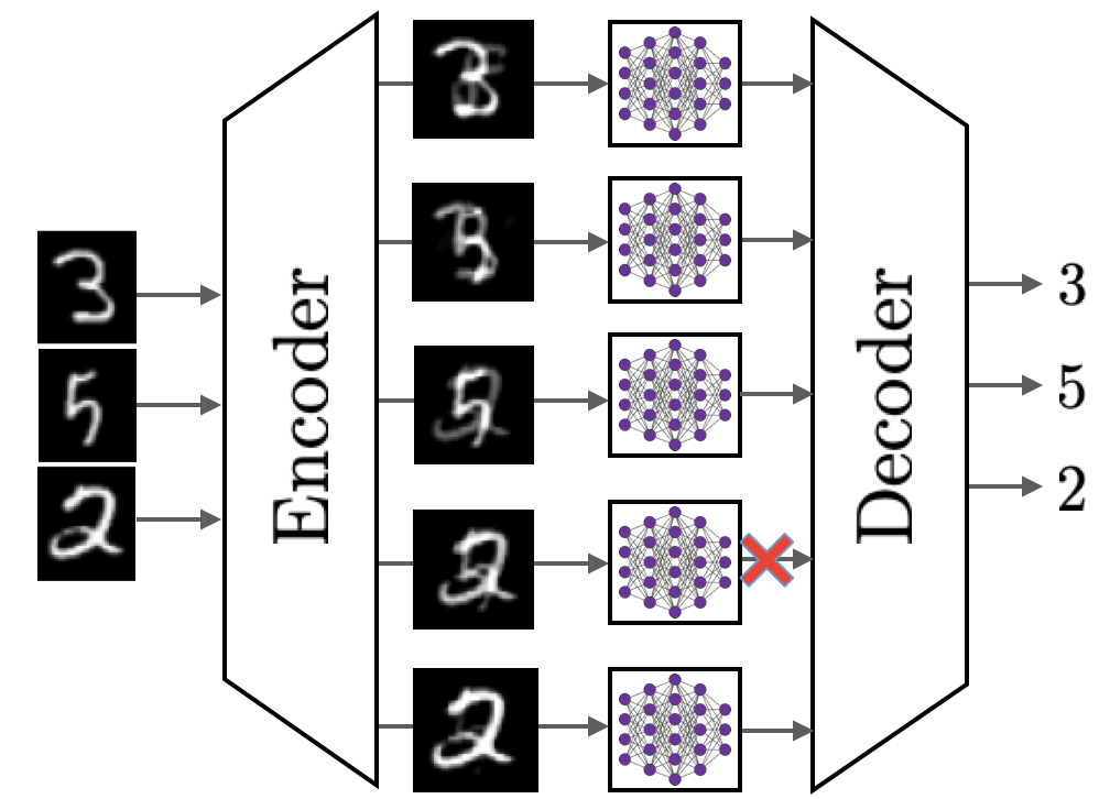
The concept of coded computing has been motivated by the success of coding in communication over unreliable channels, where instead of transmitting raw data, the transmitter sends a (linear) combination of the data, known as coded data. This redundancy in the coded data enables the receiver to recover the raw data even in the presence of errors or missing values. Similarly, coded computing includes three stages [13, 3, 11] (see Figure 1(a)):
-
(1)
The Encoding Layer in which a master node sends a (linear) combination of data, as coded data, to each worker node.
-
(2)
The Computing Layer, in which the worker nodes apply a predefined computation to their assigned coded data and send the results back to the master node.
-
(3)
The Decoding Layer, in which the master node recovers the final results from the computation results over coded data. In this stage, the decoder leverages the coded redundancy in the computation to recover the missing results of the stragglers and detect and correct the adversarial inputs.
The existing coded computing has largely built upon algebraic coding theory, drawing inspiration from the renowned Reed-Solomon code construction in communication [14], with proven straggler and Byzantine resiliency [15]. However, the coding in communication, designed for the exact recovery of the messages, built on a foundation that is inconsistent with the computational requirements of machine learning. Developing a code that preserves its specific construction while composing with computation is extremely challenging, leading to significant restrictions. Firstly, current methods are mainly restricted to specific computation functions, such as polynomials and matrix multiplication [3, 16, 17, 13, 11]. Secondly, rooted in algebraic error correction codes, existing approaches are tailored for finite field computations, leading to numerical instability when dealing with real-valued data [18, 19]. Furthermore, these methods are unsuitable for approximate, fixed-point, or floating-point computing, where exact computation is neither possible nor necessary, such as in machine learning inference or training tasks. Finally, these schemes typically have a recovery threshold, which is the minimum number of samples required to recover results from coded outputs of worker nodes [3, 13]. If the number of workers falls below this threshold, the recovery process fails entirely.
Several works have attempted to mitigate the aforementioned issues and transform the coded computing scheme into a more robust and adaptable one, applicable to a wide range of computation functions. These efforts include approximating non-polynomial functions with polynomial ones [20, 5], refining the coding mechanism to enhance stability [21, 22, 23, 24, 25], and leveraging approximation computing techniques to reduce the recovery threshold and increase recovery flexibility [26, 27, 28, 29]. However, these attempts fail to bridge the existing gap between coded computing and general distributed computing systems. The root cause of these issues lies in the fact that they are grounded in coding theory, based on a foundation that is not compatible with the requirements of large-scale machine learning. Therefore, this paper aims to address the following objective:
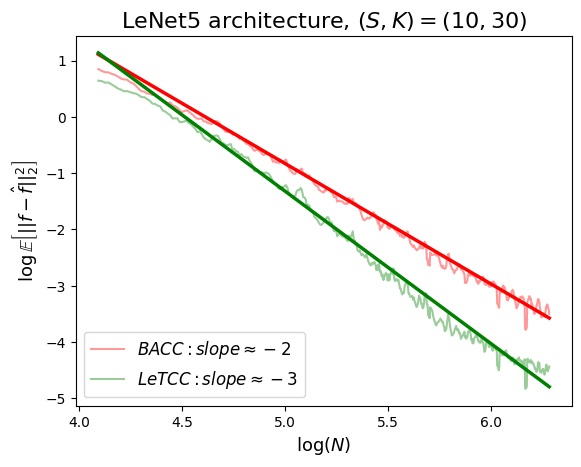
In this paper, we establish a learning-theoretic foundation for coded computing, applicable to general computations. We adopt an end-to-end system perspective, that integrates an end-to-end loss function, to find the optimum encoding and decoding functions, focusing on straggler resiliency. We show that the loss function is upper-bounded by the sum of two terms: one characterizing the generalization error of the decoder function and the other capturing the training error of the encoder function. Regularizing the decoder stage, we derive the optimal decoder in the Reproducing Kernel Hilbert space (RKHS) of second-order Sobolev functions. This provides an explicit solution for the optimum decoder function and allows us to characterize the resulting loss of the decoding stage. The decoder loss appears as a regularizing term in optimizing the encoding function and represents the norm in another RKHS. Thus, the optimum solution for the encoding function can be derived, too. We address two noise-free and noisy computation settings, for which we derive the optimal encoder and decoder and corresponding convergence rate. We prove that the proposed framework exhibits a faster convergence rate compared to the state-of-the-art and the numerical evaluations support the theoretical derivations (see Figure 1(b)).
Contributions: The main contributions of this paper are:
-
•
We develop a new foundation for coded computing, based on the theory of learning, rather than the theory of coding. We define the loss function as the square error of the computation estimation, averaged over all possible sets of at most stragglers (Section 3.1). To be able to find the best encoding and decoding functions, we bound the loss function with the summation of two terms, one characterizing the generalization error of the decoder function and the other capturing the training error of the encoder function (Section 3).
-
•
Assuming that the encoder and decoder functions reside in the Hilbert space of second-order Sobolev functions, we use the theory of RKHSs to find the optimum encoding and decoding functions and characterize the convergence rate for the expected loss in both noise-free and noisy computations (Section 4).
-
•
We have extensively evaluated the proposed scheme across different data points and computing functions including state-of-the-art deep neural networks and demonstrated that our proposed framework considerably outperforms the state-of-the-art in terms of recovery accuracy (Section 5).
2 Preliminaries and Problem Definition
2.1 Notations
Throughout this paper, uppercase and lowercase bold letters denote matrices and vectors, respectively. Coded vectors and matrices are indicated by a sign, as in . The set is denoted as and symbol denotes the cardinality of the set . Finally, we represent first, second and -th order derivative of function as , and respectively.
2.2 Problem Setting
Consider a master node and a set of workers. The master node is tasked with computing using a cluster of worker nodes, given a set of data points . Here, represents an arbitrary function, which could be a simple one-dimensional function or a complex deep neural network, and are integers. A naive approach would be to assign the computation of to one worker node for . However, some worker nodes may act as stragglers, failing to complete their tasks within the required deadline. To mitigate this issue, the master node employs coding and sends coded data points to each worker node using an encoder function. Each coded data point is a combination of raw data points. Subsequently, each worker applies the function to the received coded data and sends the result, coded results, back to the master node. The master node’s goal is to approximately recover using a decoder function, even if some worker nodes appear to be stragglers. The redundancy in the coded data and corresponding coded results enables the master node to recover the desirable results, .

3 Proposed Framework: LeTCC
Here, we propose a novel straggler-resistant Learning-Theoretic Coded Computing (LeTCC) framework for general distributed computing. As depicted in Figure 2, our framework comprises two encoding and decoding layers, with a computing layer sandwiched between them. The framework operates according to the following steps:
-
(1)
Encoding Layer: The master node fits an encoder regression function at points for fixed, distinct, and ordered values . Then, it computes the encoder function on another set of fixed, distinct, and ordered values where , with and . Subsequently, the master node sends the coded data points to worker for . Note that each coded data point is a combination of all initial points .
-
(2)
Computing Layer: Each worker node computes on its assigned input and sends the result back to the master node.
-
(3)
Decoding Layer: The master node receives the results from the non-straggler worker nodes in the set . Next, it fits a decoder regression function at points . Finally, using the function , the master node can compute as an approximation of for . Recall that .
As mentioned above, the master node selects and fixes the regression points, and , which remain constant throughout the entire process. The encoder and decoder functions are the only components subject to optimization.
Note that the computational efficiency of the encoding and decoding layers is crucial. This includes the fitting process of the encoder and decoder regression functions, as well as the computation of these regression functions at points and . If the master node’s computation time is not substantially decreased compared to computing by itself, then adopting this framework would not provide any benefits for the master node.
3.1 Objective
We view the whole scheme as a unified predictive framework that provides an approximate estimation of the values . We denote the estimator function of the LeTCC scheme as , where , , and represents the set of non-straggler worker nodes.
Let us define a random variable distributed over the set of all subsets of workers with maximum stragglers, . Also, suppose each worker node computes the function , where , are independent zero-mean noise vectors with covariance .
This enables us to define the following loss function, which evaluates the framework’s performance:
| (1) |
where to simplify the notation, represents the -norm, and . Our objective is to find and that minimize the objective function (1), which is very challenging, given that is a composition of and and the computation in the middle. Here, we take an important step to decompose these two, to gain a deeper understanding of interactions. Adding and subtracting and utilizing inequality of arithmetic and geometric means (AM-GM), one can obtain an upper bound for (1):
| (2) |
The right-hand side of (3.1) comprises two terms, which uncover an interesting interplay between the encoder and decoder regression functions. Let us elaborate on what each term corresponds to.
-
•
– The expected generalization error of the decoder regression: Recall that the master node fits a decoder regression function, , at a set of points denoted as . represents the -norm of the decoder regression function’s error on a distinct set of points , which are different from its training data . Consequently, this term provides an unbiased estimate of the decoder’s generalization error.
Given that the decoder regression function develops to estimate , the generalization error of the decoder regression is inherently tied to the properties of . This, in turn, is influenced by characteristics of both the and functions, making the a complex interplay of these two functions.
-
•
– A proxy to the training error of the encoder regression: Remember that the encoder regression is fitted at points . Consequently, the training error is calculated as . Therefore, represents the encoder training error magnified by the effect of computing function . Specifically, if is -Lipschitz, then can be upper bounded by:
(3)
4 Main Results
In this section, we investigate the proposed framework from a theoretical standpoint. We provide a detailed explanation of how to design the decoder and encoder functions and subsequently analyze the convergence rate. For simplicity, we first present the results for a one-dimensional function . All the results have been generalized to the case where as stated in Appendix C.
Suppose the regression points, , are confined to the interval and where is the RKHS of second-order Sobolev functions on interval . We review the definition and properties of Sobolev spaces in Appendix A.1.
Decoder Design: Since in the decomposition (3.1) characterizes the generalization error of the decoder function, we propose a regularized objective function for the decoder:
| (4) |
The first term in (4) corresponds to the mean squared error, while the second term characterizes the smoothness of the decoder function on the interval . Equation (4) represents a Kernel Ridge Regression problem (KRR). It can be shown that the solution of (4) has the following form [30]:
| (5) |
where is the kernel of , , and . Substituting (5) into the main objective (4), the coefficients and can be efficiently computed by optimizing a quadratic equation [31]. This solution is known as the second-order smoothing spline function. We review the theoretical properties of smoothing splines in Appendix A.2.
Let us define the following variables, which characterize the maximum and minimum distances between consecutive regression points , and . These are the points available to the decoder after removing the missing ones due to the presence of stragglers.
| (6) |
with and . The following theorems provide crucial insights for designing the encoder function as well as deriving the convergence rates.
Theorem 1 (Upper bound for noisy computation).
Consider the LeTCC framework with worker nodes and at most stragglers. Assume each worker node computes with and . Assume are equidistant in , . Also, suppose that there are constants and such that , and . If is a -Lipschitz continuous function, then:
| (7) |
with the optimal regularization parameter
| (8) |
where is a constant, and is a degree-4 polynomial of () with constant coefficients.
The proof and formula for the constant are provided in Appendix B.1.
Theorem 2 (Upper bound for noiseless computation, ).
Consider the LeTCC framework with worker nodes and at most stragglers. Assume are equidistant in , and there exist a constant that . Also, suppose . If is a -Lipschitz continuous function, then:
| (9) |
with optimal regularization parameter , where are two constants.
The proof of Theorem 2 and the detailed expressions for and , can be found in Appendix B.2. Some results in approximation theory suggest utilizing Chebyseb points of the first kind, , as regression points, as it is used in [29]. To cover those cases, we present the following corollary.
The proof can be found in
Corollary 7 in Appendix B.
Encoder Design: The upper bounds established in Theorems 1,
2 hold for all . However, they do not directly lead to a design for . To address this, we present the following theorem which bounds the , enabling us to construct without compromising the convergence rate.
Theorem 3 (Optimal encoder).
Consider a LeTCC scheme. Assume computing function is -Lipschitz continuous and . Then:
| (10) |
for some monotonically increasing function , where is constant depending on , and .
The norm is an RKHS and an equivalent norm on Sobolev space introduced by [32] (see (22) in Appendix A.1). The proof can be found in Appendix B.3. By applying the representer theorem [33], we can deduce that the optimal encoder , which minimizes the right-hand side of (10) takes the form , where , and is the kernel function of , identical to one in (5). However, due to the non-linearity of , calculating the values of the coefficients is challenging. Nevertheless, we demonstrate that the coefficients can be efficiently derived under certain mild assumptions.
Corollary 2.
In the noiseless setting, if , for some , then:
| (11) |
where is constant depending on .
See Appendix B.3.1 for the proof. Corollary 2 states that under the assumptions specified in Corollary 2, smoothing spline minimizes the upper bounds (11).
Convergence Rate: Using Theorems 1, 2, and 3, we can derive the convergence rate of the proposed scheme as stated in the following theorem.
Theorem 4 (Convergence rate).
For LeTCC scheme with worker nodes and maximum of stragglers, for the noisy computation, and for the noiseless setting.
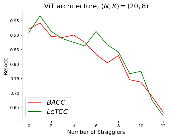
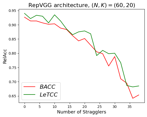
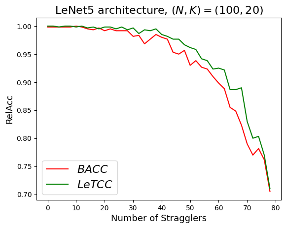
5 Experimental Results
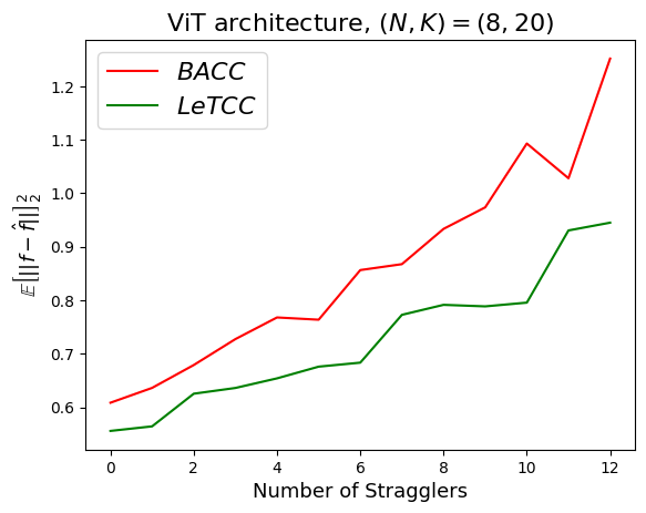
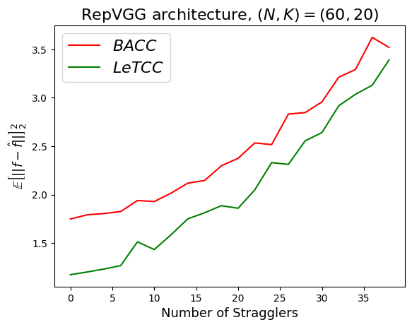
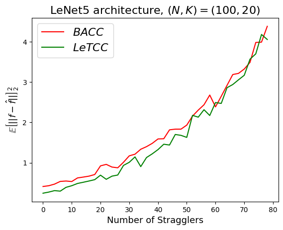
In this section, we extensively evaluate the proposed scheme across various scenarios. Our assessments involve examining multiple deep neural networks as computing functions and exploring the impact of different numbers of stragglers on the scheme’s efficiency. The experiments are run using PyTorch [34] in a single GPU machine. We evaluate the performance of the LeTCC scheme in three different model architectures:
- •
-
•
Deep model with low-dimensional output: In this scenario, we evaluate the proposed scheme when the function is a deep neural network trained on color images in CIFAR-10 [37] dataset. We use the recently introduced RepVGG [38] network with around million parameters which was trained on CIFAR-10111The pre-trained weights can be found here..
-
•
Deep model with high-dimensional output: Finally, we demonstrate the performance of the LeTCC scheme in a scenario where the input and output of the computing function are high-dimensional, and the function is a relatively large neural network. We consider the Vision Transformer (ViT) [39] as one of the state-of-the-art base neural networks in computer vision for our prediction model, with more than million parameters (in the base version). The network was trained and fine-tuned on the ImageNet-1K dataset [40]222We use the official PyTorch pre-trained ViT network from here..
We use the output of the last softmax layer of each model as the output.
| LeNet5 | RepVGG | ViT | ||||
| Method | MSE | RelAcc | MSE | RelAcc | MSE | RelAcc |
| BACC | 2.55 0.43 | 0.92 0.04 | 2.44 0.38 | 0.83 0.05 | 0.68 0.13 | 0.90 0.07 |
| LeTCC | 2.18 0.51 | 0.94 0.04 | 2.04 0.42 | 0.87 0.05 | 0.62 0.11 | 0.94 0.06 |
Hyper-parameters: The entire encoding and decoding process is the same for different functions, as we adhere to a non-parametric approach. The sole hyper-parameters involved are the two smoothing parameters () which are determined using cross-validation and greed search over different values of the smoothing parameters.
Baseline: We compare LeTCC with the Berrut approximate coded computing (BACC) introduced by [29] as the state-of-the-art coded computing scheme for general computing. The BACC framework is used in [29] for training neural networks and in [41] for inference.
Interpolation Points: We choose Chebyshev points of the first and second kind, and , for fair comparison with [29].
Evaluation Metrics: We employ two evaluation metrics to assess the performance of the proposed framework: Relative Accuracy (RelAcc) and Mean Squared Error (MSE). RelAcc is defined as the ratio of the base model’s prediction accuracy to the accuracy of the estimated model on the initial data points. MSE, on the other hand, is our main loss defined in (1) which measures the empirical average of the mean squared difference over multiple batches of and non-straggler set , , where is the distribution of input data.
Performance Evaluation:
Table 1 presents both MSE and RelAcc metrics side by side.
The results demonstrate that LeTCC outperforms BACC across various architectures and configurations, with an average improvement of 15%, 17%, and 9% in MSE for LeNet, RepVGG, and ViT architectures, respectively, and a 2%, 5%, and 4% enhancement in RelAcc.
In the subsequent analysis, we assess the performance of LeTCC in comparison to BACC for a diverse range of stragglers. For a constant number of stragglers, we execute both schemes with the same set of input data points and the same set of stragglers multiple times and record the average RelAcc and MSE metrics. Figure 3 presents the performance of both schemes on three model architectures. As depicted in Figure 3, the proposed scheme consistently outperforms BACC across nearly all values for the number of stragglers.
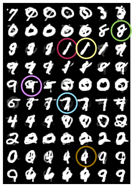
Coded Points: We also compare the coded points sent to the workers in LeTCC and BACC schemes. The results, shown in Figure 4, demonstrate that BACC coded samples exhibit high-frequency noise which causes the scheme to approximate the original prediction worse than LeTCC.
6 Related Work
Coded computing was initially introduced to tackle the challenges of distributed computation, particularly the existence of stragglers or slow workers, and also faulty or adversarial nodes. Traditional approaches to deal with stragglers primarily rely on repetition [42, 1, 43, 44, 45, 46], where each task is assigned to multiple workers either proactively or reactively. Recently, coded computing approaches have reduced the overhead of repetition by leveraging coding theory and embedding redundancy in the worker’s input data [29, 3, 13, 26, 47, 48, 49, 50, 51]. This technique, which mainly relies on theory of coding, has been developed for specific types of structured computations, such as polynomial computation and matrix multiplication [13, 3, 52, 17, 53, 48, 12, 7, 54]. Recently, there have been attempts to generalize coded computing for general computations [29, 55, 4, 5]. Towards extending the application of coding computing to machine learning computation, Kosaian et al. [55] suggest training a neural network to predict coded outputs from coded data points. However, the scheme of Kosaian et al. [55] requires a complex training process and tolerates only one straggler. In another work, Jahani-Nezhad and Maddah-Ali [29] proposes BACC, a model-agnostic and numerically stable framework for general computations. They successfully employed BACC to train neural networks on a cluster of workers, while tolerating a larger number of stragglers. Building on the BACC framework, Soleymani et al. [41] introduced ApproxIFER scheme, as a straggler resistance and Byzantine-robust prediction serving system. However, the scheme of BACC uses a reasonable rational interpolation (Berrut interpolation [56]), off the shelf, for encoding and decoding, without considering any end-to-end cost function to optimize. In contrast, we theoretically formalize a new foundation of coded computing grounded in learning theory, which can be naturally used for machine learning applications.
7 Conclusions and Future Work
In this paper, we developed a new foundation for coded computing based on learning theory, contrasting with existing works that rely on coding theory and use metrics like minimum distance and recovery threshold for design. This shift in foundations removes barriers to using coded computing for machine learning applications, allows us to design optimal encoding and decoding functions, and achieves convergence rates that outperform the state of the art. Moreover, the experimental evaluations validate the theoretical guarantees. While this work focuses on straggler mitigation, future work will extend our proposed scheme to achieve Byzantine robustness and privacy, offering promising avenues for further research.
References
- Dean and Barroso [2013] Jeffrey Dean and Luiz André Barroso. The tail at scale. Communications of the ACM, 56(2):74–80, 2013.
- Gupta et al. [2018a] Vipul Gupta, Shusen Wang, Thomas Courtade, and Kannan Ramchandran. Oversketch: Approximate matrix multiplication for the cloud. In 2018 IEEE International Conference on Big Data (Big Data), pages 298–304. IEEE, 2018a.
- Yu et al. [2019] Qian Yu, Songze Li, Netanel Raviv, Seyed Mohammadreza Mousavi Kalan, Mahdi Soltanolkotabi, and Salman A Avestimehr. Lagrange coded computing: Optimal design for resiliency, security, and privacy. In The 22nd International Conference on Artificial Intelligence and Statistics, pages 1215–1225. PMLR, 2019.
- So et al. [2020a] Jinhyun So, Basak Guler, and Amir Salman Avestimehr. A scalable approach for privacy-preserving collaborative machine learning. In Advances in Neural Information Processing Systems, volume 33, pages 8054–8066, 2020a.
- So et al. [2021] Jinhyun So, Başak Güler, and Amir Salman Avestimehr. CodedPrivateML: A fast and privacy-preserving framework for distributed machine learning. IEEE Journal on Selected Areas in Information Theory, 2(1):441–451, 2021.
- Jia and Jafar [2021] Zhuqing Jia and Syed Ali Jafar. On the capacity of secure distributed batch matrix multiplication. IEEE Transactions on Information Theory, 67(11):7420–7437, 2021.
- Aliasgari et al. [2020] Malihe Aliasgari, Osvaldo Simeone, and Jörg Kliewer. Private and secure distributed matrix multiplication with flexible communication load. IEEE Transactions on Information Forensics and Security, 2020.
- Kim and Lee [2019] Minchul Kim and Jungwoo Lee. Private secure coded computation. In 2019 IEEE International Symposium on Information Theory (ISIT), pages 1097–1101. IEEE, 2019.
- Chang and Tandon [2019] Wei-Ting Chang and Ravi Tandon. On the upload versus download cost for secure and private matrix multiplication. In 2019 IEEE Information Theory Workshop (ITW), pages 1–5. IEEE, 2019.
- Chang and Tandon [2018] Wei-Ting Chang and Ravi Tandon. On the capacity of secure distributed matrix multiplication. In 2018 IEEE Global Communications Conference (GLOBECOM), pages 1–6, 2018.
- Yu et al. [2020a] Qian Yu, Mohammad Ali Maddah-Ali, and A Salman Avestimehr. Straggler mitigation in distributed matrix multiplication: Fundamental limits and optimal coding. IEEE Transactions on Information Theory, 66(3):1920–1933, 2020a.
- D’Oliveira et al. [2020] Rafael G.L. D’Oliveira, Salim El Rouayheb, and David Karpuk. GASP codes for secure distributed matrix multiplication. IEEE Transactions on Information Theory, 66(7):4038–4050, 2020.
- Yu et al. [2017] Qian Yu, Mohammad Maddah-Ali, and Salman Avestimehr. Polynomial codes: an optimal design for high-dimensional coded matrix multiplication. Advances in Neural Information Processing Systems, 30, 2017.
- Reed and Solomon [1960] Irving S Reed and Gustave Solomon. Polynomial codes over certain finite fields. Journal of the society for industrial and applied mathematics, 8(2):300–304, 1960.
- Guruswami et al. [2022] Venkatesan Guruswami, Atri Rudra, and Madhu Sudan. Essential Coding Theory. Draft is Available, 2022.
- Lee et al. [2018] K. Lee, M. Lam, R. Pedarsani, D. Papailiopoulos, and K. Ramchandran. Speeding up distributed machine learning using codes. IEEE Transactions on Information Theory, 64(3):1514–1529, 2018.
- Lee et al. [2017] K. Lee, C. Suh, and K. Ramchandran. High-dimensional coded matrix multiplication. In Proceedings of IEEE International Symposium on Information Theory (ISIT), pages 2418–2422, 2017.
- Gautschi and Inglese [1987] Walter Gautschi and Gabriele Inglese. Lower bounds for the condition number of vandermonde matrices. Numerische Mathematik, 52(3):241–250, 1987.
- Golub and Van Loan [2013] Gene H. Golub and Charles F. Van Loan. Matrix computations. JHU press, 2013.
- So et al. [2020b] Jinhyun So, Basak Guler, and Salman Avestimehr. A scalable approach for privacy-preserving collaborative machine learning. Advances in Neural Information Processing Systems, 33:8054–8066, 2020b.
- Subramaniam et al. [2019] Adarsh M. Subramaniam, Anoosheh Heidarzadeh, and Krishna R. Narayanan. Random Khatri-Rao-product codes for numerically-stable distributed matrix multiplication. CoRR, abs/1907.05965, 2019.
- Ramamoorthy and Tang [2022] Aditya Ramamoorthy and Li Tang. Numerically stable coded matrix computations via circulant and rotation matrix embeddings. IEEE Transactions on Information Theory, 68(4):2684–2703, 2022.
- Das et al. [2021] Anindya Bijoy Das, Aditya Ramamoorthy, and Namrata Vaswani. Efficient and robust distributed matrix computations via convolutional coding. IEEE Transactions on Information Theory, 67(9):6266–6282, 2021.
- Soleymani et al. [2021] Mahdi Soleymani, Hessam Mahdavifar, and Amir Salman Avestimehr. Analog Lagrange coded computing. IEEE Journal on Selected Areas in Information Theory, 2(1):283–295, 2021.
- Fahim and Cadambe [2021a] Mohammad Fahim and Viveck R Cadambe. Numerically stable polynomially coded computing. IEEE Transactions on Information Theory, 67(5):2758–2785, 2021a.
- Jahani-Nezhad and Maddah-Ali [2021] Tayyebeh Jahani-Nezhad and Mohammad Ali Maddah-Ali. CodedSketch: A coding scheme for distributed computation of approximated matrix multiplication. IEEE Transactions on Information Theory, 67(6):4185–4196, 2021.
- Gupta et al. [2018b] Vipul Gupta, Shusen Wang, Thomas Courtade, and Kannan Ramchandran. OverSketch: Approximate matrix multiplication for the cloud. In 2018 IEEE International Conference on Big Data (Big Data), pages 298–304, 2018b.
- Gupta et al. [2020] Vipul Gupta, Swanand Kadhe, Thomas Courtade, Michael W. Mahoney, and Kannan Ramchandran. Oversketched Newton: Fast convex optimization for serverless systems. In 2020 IEEE International Conference on Big Data (Big Data), pages 288–297, 2020.
- Jahani-Nezhad and Maddah-Ali [2022] Tayyebeh Jahani-Nezhad and Mohammad Ali Maddah-Ali. Berrut approximated coded computing: Straggler resistance beyond polynomial computing. IEEE Transactions on Pattern Analysis and Machine Intelligence, 45(1):111–122, 2022.
- Duchon [1977] Jean Duchon. Splines minimizing rotation-invariant semi-norms in sobolev spaces. In Constructive Theory of Functions of Several Variables: Proceedings of a Conference Held at Oberwolfach April 25–May 1, 1976, pages 85–100. Springer, 1977.
- Wahba [1975] Grace Wahba. Smoothing noisy data with spline functions. Numerische mathematik, 24(5):383–393, 1975.
- Kimeldorf and Wahba [1971] George Kimeldorf and Grace Wahba. Some results on tchebycheffian spline functions. Journal of mathematical analysis and applications, 33(1):82–95, 1971.
- Mohri et al. [2018] Mehryar Mohri, Afshin Rostamizadeh, and Ameet Talwalkar. Foundations of machine learning. MIT press, 2018.
- Paszke et al. [2019] Adam Paszke, Sam Gross, Francisco Massa, Adam Lerer, James Bradbury, Gregory Chanan, Trevor Killeen, Zeming Lin, Natalia Gimelshein, Luca Antiga, et al. Pytorch: An imperative style, high-performance deep learning library. Advances in neural information processing systems, 32, 2019.
- LeCun et al. [1998] Yann LeCun, Léon Bottou, Yoshua Bengio, and Patrick Haffner. Gradient-based learning applied to document recognition. Proceedings of the IEEE, 86(11):2278–2324, 1998.
- LeCun et al. [2010] Yann LeCun, Corinna Cortes, Chris Burges, et al. MNIST handwritten digit database, 2010.
- Krizhevsky et al. [2009] Alex Krizhevsky, Geoffrey Hinton, et al. Learning multiple layers of features from tiny images. 2009.
- Ding et al. [2021] Xiaohan Ding, Xiangyu Zhang, Ningning Ma, Jungong Han, Guiguang Ding, and Jian Sun. Repvgg: Making vgg-style convnets great again. In Proceedings of the IEEE/CVF conference on computer vision and pattern recognition, pages 13733–13742, 2021.
- Dosovitskiy et al. [2020] Alexey Dosovitskiy, Lucas Beyer, Alexander Kolesnikov, Dirk Weissenborn, Xiaohua Zhai, Thomas Unterthiner, Mostafa Dehghani, Matthias Minderer, Georg Heigold, Sylvain Gelly, et al. An image is worth 16x16 words: Transformers for image recognition at scale. arXiv preprint arXiv:2010.11929, 2020.
- Deng et al. [2009] Jia Deng, Wei Dong, Richard Socher, Li-Jia Li, Kai Li, and Li Fei-Fei. Imagenet: A large-scale hierarchical image database. In 2009 IEEE conference on computer vision and pattern recognition, pages 248–255. Ieee, 2009.
- Soleymani et al. [2022] Mahdi Soleymani, Ramy E Ali, Hessam Mahdavifar, and A Salman Avestimehr. ApproxIFER: A model-agnostic approach to resilient and robust prediction serving systems. In Proceedings of the AAAI Conference on Artificial Intelligence, volume 36, pages 8342–8350, 2022.
- Zaharia et al. [2008] Matei Zaharia, Andy Konwinski, Anthony D Joseph, Randy H Katz, and Ion Stoica. Improving mapreduce performance in heterogeneous environments. In Osdi, volume 8, page 7, 2008.
- Suresh et al. [2015] Lalith Suresh, Marco Canini, Stefan Schmid, and Anja Feldmann. C3: Cutting tail latency in cloud data stores via adaptive replica selection. In 12th USENIX Symposium on Networked Systems Design and Implementation (NSDI 15), pages 513–527, 2015.
- Shah et al. [2015] Nihar B Shah, Kangwook Lee, and Kannan Ramchandran. When do redundant requests reduce latency? IEEE Transactions on Communications, 64(2):715–722, 2015.
- Gardner et al. [2015] Kristen Gardner, Samuel Zbarsky, Sherwin Doroudi, Mor Harchol-Balter, and Esa Hyytia. Reducing latency via redundant requests: Exact analysis. ACM SIGMETRICS Performance Evaluation Review, 43(1):347–360, 2015.
- Chaubey and Saule [2015] Manmohan Chaubey and Erik Saule. Replicated data placement for uncertain scheduling. In 2015 IEEE International Parallel and Distributed Processing Symposium Workshop, pages 464–472. IEEE, 2015.
- Li et al. [2018] Songze Li, Seyed Mohammadreza Mousavi Kalan, Amir Salman Avestimehr, and Mahdi Soltanolkotabi. Near-optimal straggler mitigation for distributed gradient methods. In 2018 IEEE International Parallel and Distributed Processing Symposium Workshops (IPDPSW), pages 857–866. IEEE, 2018.
- Das et al. [2019] Anindya B Das, Aditya Ramamoorthy, and Namrata Vaswani. Random convolutional coding for robust and straggler resilient distributed matrix computation. arXiv preprint arXiv:1907.08064, 2019.
- Ramamoorthy et al. [2020] Aditya Ramamoorthy, Anindya Bijoy Das, and Li Tang. Straggler-resistant distributed matrix computation via coding theory: Removing a bottleneck in large-scale data processing. IEEE Signal Processing Magazine, 37(3):136–145, 2020.
- Karakus et al. [2017] Can Karakus, Yifan Sun, Suhas Diggavi, and Wotao Yin. Straggler mitigation in distributed optimization through data encoding. Advances in Neural Information Processing Systems, 30, 2017.
- Tandon et al. [2017] R. Tandon, Q. Lei, A. G. Dimakis, and N. Karampatziakis. Gradient coding: Avoiding stragglers in distributed learning. In Proceedings of the 34th International Conference on Machine Learning (ICML), pages 3368–3376, Sydney, Australia, August 2017.
- Ramamoorthy and Tang [2021] Aditya Ramamoorthy and Li Tang. Numerically stable coded matrix computations via circulant and rotation matrix embeddings. IEEE Transactions on Information Theory, 68(4):2684–2703, 2021.
- Yu et al. [2020b] Qian Yu, Mohammad Ali Maddah-Ali, and Amir Salman Avestimehr. Straggler mitigation in distributed matrix multiplication: Fundamental limits and optimal coding. IEEE Transactions on Information Theory, 66(3):1920–1933, 2020b.
- Fahim and Cadambe [2021b] Mohammad Fahim and Viveck R. Cadambe. Numerically stable polynomially coded computing. IEEE Transactions on Information Theory, 67(5):2758–2785, 2021b.
- Kosaian et al. [2019] Jack Kosaian, KV Rashmi, and Shivaram Venkataraman. Parity models: A general framework for coding-based resilience in ml inference. arXiv preprint arXiv:1905.00863, 2019.
- Berrut [1988] J-P Berrut. Rational functions for guaranteed and experimentally well-conditioned global interpolation. Computers & Mathematics with Applications, 15(1):1–16, 1988.
- Leoni [2024] Giovanni Leoni. A first course in Sobolev spaces, volume 181. American Mathematical Society, 2024.
- Adams and Fournier [2003] Robert A Adams and John JF Fournier. Sobolev spaces. Elsevier, 2003.
- Berlinet and Thomas-Agnan [2011] Alain Berlinet and Christine Thomas-Agnan. Reproducing kernel Hilbert spaces in probability and statistics. Springer Science & Business Media, 2011.
- Wahba [1990] Grace Wahba. Spline models for observational data. SIAM, 1990.
- Ragozin [1983] David L Ragozin. Error bounds for derivative estimates based on spline smoothing of exact or noisy data. Journal of approximation theory, 37(4):335–355, 1983.
- Utreras [1988] Florencio I Utreras. Convergence rates for multivariate smoothing spline functions. Journal of approximation theory, 52(1):1–27, 1988.
Appendix A Preliminaries
A.1 Sobolev spaces and Sobolev norms
Let be an open interval in and be a positive integer. We denote by the class of all measurable functions that satisfy:
| (12) |
where . The space can be endowed with the following norm, known as norm:
| (13) |
for and
| (14) |
for . Additionally, a function is in if it lies in for all compact subsets .
Definition 1.
(Sobolev Space): The Sobolev space is the space of all functions such that all weak derivatives of order , denoted by , belong to for . This space is endowed with the norm:
| (15) |
for and
| (16) |
for .
Subsequently, let us define Sobolev space as the space of all functions with all weak derivatives of order belonging to for . and are defined similar to (15) and (16) respectively, using instead of .
The next theorem provides an upper bound for norm of functions in the Sobolev space, which plays a crucial role in the proof of the main theorems of the paper.
Theorem 5.
Note that in Theorem 5 is the length of the interval .
Corollary 3.
Suppose and be an open interval. If then:
| (18) |
Proof.
Corollary 4.
Theorem 5 remains true when :
Proof.
Equivalent norms. There have been various norms defined on Sobolev spaces in the literature that are equivalent to (15) (see [58], [59, Ch. 7], and [60, Sec. 10.2]). Note that two norms are equivalent if there exist positive constants such that . The equivalent norm that we are interested in is the one introduced in [32]. Let . The Sobolev space can be endowed by the norm
| (22) |
The following lemma derives the equivalency constants () for the norms and .
Lemma 1.
Let an arbitrary interval in . Then for every :
| (23) | ||||
| (24) |
Proof.
By expanding around the point and using the integral reminder form of Taylor’s expansion, for every :
Thus:
| (25) |
where (a) follows from the , (b) is based on Cauchy-Schwarz inequality, and (c) is due to . Following the same steps as (A.1), we have:
| (26) |
Integrating both sides of (26) we have:
| (27) |
where (a) is based on adding a positive term . Based on the (A.1),(A.1) we have:
| (28) |
where (a) follows by integrating both sides of (A.1) and (b) is due to (26). Using (A.1) and (A.1) and the fact that , we have:
| (29) |
For the other side, using the same steps as in (A.1), we have:
| (30) |
where (a) is because of , (b) follows from Cauchy-Schwarz inequality, and (c) is due to . Integrating both sides of (A.1), we have
| (31) |
where (a) follows by a change of variable from to and (b) follows by adding a positive term to the right side. Thus, (A.1) directly results in
| (32) |
Following same steps as (A.1) and (32) results in
| (33) |
Considering the fact that we complete the proof:
| (34) |
∎
Corollary 5.
Based on Lemma 1, for we have
| (35) |
Corollary 6.
The result of Lemma 1 remains valid for multi-dimensional cases, where , for some .
A.2 Smoothing Splines
Consider the data model for , where , , . Assume , then the solution of the following optimization problem is known as smoothing spline:
| (36) |
where .
Proposition 1.
Based on 1, there exists a kernel associated with the Sobolev norm such that for any , we have:
| (38) |
The solution of (36) has the following form [60, 30]:
| (39) |
where are basis functions of the space of all polynomials with degree less than or equal to , and for . Substituting into (36) and optimizing over , one can show that:
| (40) |
where , with are defined as:
| (41) |
Equation (40) states that the smoothing spline fitted on the data points is a linear operator, i.e., for .
To characterize the estimation error of the smoothing spline, , we need to define two variables analogous to those in (6), which quantify the minimum and maximum consecutive distance of the regression points .
| (42) |
Note that the boundary points are defined as in (42). The following theorem offers an upper bound for the -th derivative of the smoothing spline estimator error function in the absence of noise ().
Theorem 6.
([61, Theorem 4.10]) Consider data model with belong to for . Let
where is a degree polynomial of with positive weights and D(m) is a function of . Then for each and any , there exist a function such that:
| (43) |
Note that in (43). In the presence of noise, where , we can leverage the linearity of the smoothing spline operator and the mutual independence of the noises to conclude that:
| (44) |
where . The first term in (A.2) can be upper bounded using Theorem 6. The following theorem provides an upper bound for the second term when is bounded:
Theorem 7.
([62, Section 5]) Consider data model , where and for . Assume there exist a constant such that . Then for each , there exist a constant and function such that:
| (45) |
for and .
Appendix B Proof of Theorems
Recall from (3.1) that , where
| (46) | |||
| (47) |
We begin by deriving a general intermediate bound for and which will be a key component in the proofs of Theorems 2 and 1. The subsequent subsections will then provide the remaining details to complete the proofs of these theorems.
Lemma 2.
Let be a -Lipschitz continuous function. Then:
| (48) |
Proof.
Using Lipschitz property, we have:
| (49) |
∎
As previously mentioned, represents the expected generalization error of the decoder function. To leverage the results from Theorems 6 and 7 we must establish that the composition of with the encoder belongs to the Sobolev space .
Lemma 3.
Let be a -Lipschitz continuous function with and be an open interval. If then .
Proof.
Let us define . Thus and is -Lipschitz. Using Lipschitz property
| (50) |
Integrating both sides of (50):
| (51) |
where (a) follows by . Given that is -Lipschitz, its derivative is bounded in the -norm, i.e., . Thus
| (52) |
where (a) follows by chain rule and (b) follows by .
| (53) |
where (a) follows by chain rule, (b) and (d) follow by Cauchy-Schwartz inequality, (c) follows by and (e) follows by . Equations (51), (52), and (B) prove that . Observe that is bounded and every constant function lies in the . Therefore, we can conclude that . ∎
Let us define the function . Based on Lemma 3, given that , thus . The following lemmas upper bound the discrete sum present in (46) with its continuous integral.
Lemma 4.
Let be an open bounded interval on , for . Then:
| (54) |
Proof.
| (55) | ||||
| (56) |
where (a) follows by with , (b) follows by Lagrange’s mean value theorem with , and (c) follows by . Thus:
∎
Corollary 7.
Let and be the Chebyshev points of the first kind for . Then:
| (57) |
Proof.
Let us reformulate the first kind of Chebysev points based on equidistant points for :
| (58) |
where . Applying Lemma 4 to function , we have:
| (59) |
where (a) is due to the fact that . For we have:
| (60) |
We can define a new variable denoted by and rewrite the LHS with the fact that :
| (61) |
So, the integral range remains symmetric around zero. Thus, we have:
| (62) |
Therefore,
| (63) |
∎
Using Lemma 4 we have:
| (64) |
In the subsequent lemmas, we offer an upper bound for the second term in (64).
Lemma 5.
If , then:
| (65) |
Proof.
Assume . Therefore, for . Thus
| (66) |
where (a) and (b) are followed by the triangle and Cauchy-Schwartz inequalities respectively. Integrating the square of both sides over the interval yields:
| (67) |
where (a) follows by . On the other side, we have the following for every :
| (68) |
Therefore, we have a similar inequality:
| (69) |
Using (67) and (69) completes the proof:
| (70) | ||||
| (71) |
Thus, if exists, the proof is complete. In the next step, we prove the existence of such that . Recall that and is the solution of (4). Assume there is no such . Since , then is continuous. Therefore, if there exist such that and , then the intermediate value theorem states that there exists such that . Thus, or for all . Without loss of generality, assume the first case where for all . It means that , . Let us define
Let . Note that . However,
| (72) |
where (a) follows from and for all . This leads to a contradiction since it implies that is not the solution of the (4). Therefore, our initial assumption must be wrong. Thus, there exists such that . ∎
Lemma 6.
Let . For we have:
| (73) |
and
| (74) |
Proof.
Building upon Lemma 6, we can proceed from (64) to establish the desired result:
| (76) | |||||
Since , we have . Assume there exist constants and that and . Defining , we have:
| (77) |
where (a) follows from Cauchy-Schwartz inequality.
B.1 Proof of Theorem 1
As previously mentioned, is a second-order smoothing spline fitted on , where is a set of non-straggler worker nodes and is a set of noisy computation values form non-straggler workers. Let us define representing the smoothing spline operator of the decoder. Using the decomposition (A.2) we have:
| (78) | |||||
where and . Let us define the following variables analogous to those in (6):
| (79) |
Since there are at most stragglers among worker nodes, . Therefore, is bounded. Additionally, since and , then implies that both and has the same order of . Thus, there exists a constant such that and correspondingly .
Applying Theorems 7 and 6 with , we have
| (80) |
and
| (81) |
where , , and as defined in Theorems 6 and 7. Since , we have:
| (82) |
where , is a degree three polynomial of , and (a) follows from the fact that . Substituting in (80), we have:
| (83) |
where (a) follows from the fact that , as assumed in Theorem 7 and (b) is by definition . An analogous upper bound can be derived for as
| (84) |
where (a) is by definition and (b) is by definition . Using the last upper bound for in (B) and combining the results from (B.1) and (B.1), we can conclude that:
| (85) | |||||
where (a) follows by the definitions and , (b) is due to and , and (c) follow from . By defining which is a degree-4 polynomial with the coefficients depend on as well as , we can conclude that:
| (86) |
Optimizing over , the optimum is:
| (87) |
By substituting the expression for into (86), defining and using previously driven upper bound for in Lemma 2, the proof is completed.
B.2 Proof of Theorem 2
In the noiseless setting, the expectation is just over :
| (88) |
Using the same steps as Appendix B, we have:
| (89) | |||||
| (90) | |||||
Note that both (89) and (B.2) are increasing function of and the upper bound of in (B) is increasing function of both and . Therefore, minimizes the right-hand side of (B) in the noiseless setting. Putting , we have:
| (91) | |||||
where and (a) follows from . Therefore, defining and as well as using Lemma 2 complete the proof.
B.3 Proof of Theorem 3
The upper bound provided in Theorems 1 and 2 depend on with the exponent and respectively. Applying the chain rule, we can show that:
| (92) |
where (a) follows from applying the chain rule, (b) and (d) follow from the chain rule, (c) is due to the Lipschitz property and the assumption that , (e) follows from adding positive terms to and to form Sobolev norm as stated in (15), (f) is due to Corollary 5 and Proposition 1, and (g) follows from the definition .
Combining (B.3) with Theorems 2 and 1 we have
| (93) |
for the noiseless setting and
| (94) |
for the noisy setting, where the parameters and are as follows:
| (95) | ||||
| (96) |
Noted that since and are monotonically increasing in , its composition is monotonically increasing as well. Moreover, and share the same exponent of as in Theorems 2 and 1, respectively. Consequently, the provided upper bound does not compromise the convergence rate.
B.3.1 Proof of Corollary 2
B.4 Proof of Theorem 4
Appendix C High-dimensional computing function
Let us consider the general case where is a vector-valued function, where each component function is -Lipschitz continuous. Based on (3.1), we have:
Let us define the following objective for the decoder function:
| (100) |
The solution to (100), denoted as , is a vector-valued function, where each component is a smoothing spline function fitted to the data points . As a result, By defining and scaling up all upper bounds for by a factor of , all previous results and theorems seamlessly extend to high-dimensional computing functions.
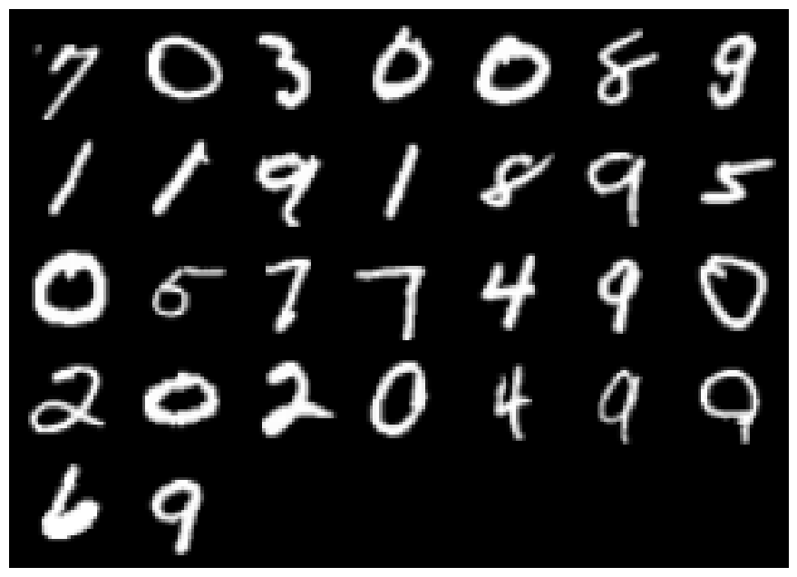
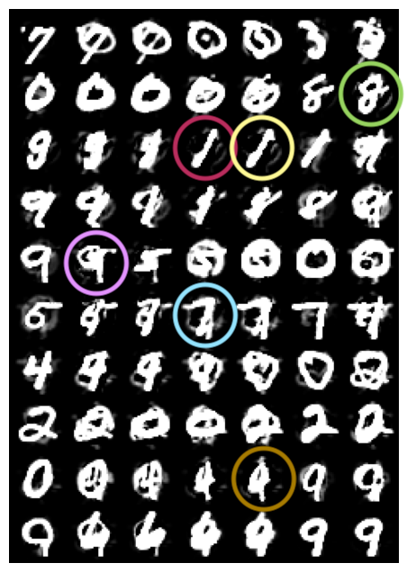
Appendix D Coded data points
Figures 4(b) and 4(c) display coded samples generated by BACC and LeTCC, respectively, derived from the same initial data points depicted in Figure 4(a). These samples are presented for the MNIST dataset with parameters . From the figures, it is apparent (Specifically in paired ones that are shown with the same color) that while both schemes’ coded samples are a weighted combination of multiple initial samples, BACC’s coded samples exhibit high-frequency noise. This observation suggests that LeTCC regression functions produce more refined coded samples without any disruptive noise.