Phasor-Driven Acceleration for FFT-based CNNs

Abstract

Recent research in deep learning (DL) has investigated the use of the Fast Fourier Transform (FFT) to accelerate the computations involved in Convolutional Neural Networks (CNNs) by replacing spatial convolution with element-wise multiplications on the spectral domain. These approaches mainly rely on the FFT to reduce the number of operations, which can be further decreased by adopting the Real-Valued FFT. In this paper, we propose using the phasor form—a polar representation of complex numbers, as a more efficient alternative to the traditional approach. The experimental results, evaluated on the CIFAR-10, demonstrate that our method achieves superior speed improvements of up to a factor of 1.376 (average of 1.316) during training and up to 1.390 (average of 1.321) during inference when compared to the traditional rectangular form employed in modern CNN architectures. Similarly, when evaluated on the CIFAR-100, our method achieves superior speed improvements of up to a factor of 1.375 (average of 1.299) during training and up to 1.387 (average of 1.300) during inference. Most importantly, given the modular aspect of our approach, the proposed method can be applied to any existing convolution-based DL model without design changes.

I Introduction

CNNs have become the cornerstone of the recent advancements in computer vision applications, leading the way for models with better-than-human performance across various tasks, viz. image classification, image enhancement, and object detection, recognition, and tracking. However, training the state-of-the-art Deep Convolutional Neural Networks (DCNNs) requires large-scale datasets, such as ImageNet [1], to be processed many times over, thus making the computation speed of the model a critical aspect.

Traditionally, DCNNs are known to take considerable amounts of time to be trained, even when powered by Graphical Processing Units (GPUs): AlexNet [2] takes 5-6 days when trained on 2x NVIDIA GTX 580 3GB GPUs; VGG [3] variants takes 2-3 weeks on 4x NVIDIA Titan Black GPUs; Inception-V3 [4] and ResNet-50 [5] take, respectively, 25 and 18 days on a single NVIDIA Quadro P4000 GPU, as found in [6]. Hence, recent studies show that with abundant computational power, the training time can be reduced by orders of several magnitude: ResNet-50 takes 20 minutes to be trained on 2048x Intel Xeon Phi 7250 [7]. The training time of ResNet-50 is lowered to 122 seconds on 3456x NVIDIA Tesla V100 [8]; and further reduced to 74.7 seconds on 2048x NVIDIA Tesla V100 [9].

Although the computational time required by DCNN models can be massively reduced by using clusters with a high number of processing units, such approaches do not focus on accelerating computations by reducing the number of operations on an algorithmic level. Researching techniques to lower the computational requirements of DCNNs is still a highly demanding task due to two unique reasons: (a) not every application has access to abundant computational power since GPUs are still an expansive resource and edge applications might be restricted to a couple of CPU cores; (b) such techniques are platform agnostic; hence, they can also be incorporated into applications that have many processing units to further reduce their computational time and energy consumption footprint.

Several strategies have been proposed to accelerate DCNNs in literature. For instance, the work in [10] proposes a taxonomy of CNN acceleration methods, which categorizes the techniques present in the literature in three main levels: structure level, algorithm level, and implementation level. As highlighted in that taxonomy, three approaches are used to obtain efficient convolution operations at the algorithm level, as listed below.

• im2col-based algorithms, which are based on the GEneral Matrix Multiplication (GEMM) function of the Basic Linear Algebra Subprograms (BLAS) library [11];

• Winograd’s algorithms [12], which are capable of computing minimal arithmetic complexity for convolutions of small kernels and mini-batches sizes; and

• FFT-based algorithms [13, 14], which are based on the convolution theorem of the Fourier domain.

These three methods are well-established; they, and their variations, serve as canonical approaches within the NVIDIA cuDNN library [15]. The vast majority of CNN applications use cuDNN indirectly through frameworks, such as PyTorch [16], which by defaults causes the cuDNN to benchmark the convolution algorithms and select the fastest. For instance, PyTorch’s benchmark process relies on cuDNN functions like cudnnFindConvolutionForwardAlgorithm and cudnnFindConvolutionBackwardDataAlgorithm. Hence, these three algorithms are of extreme importance, and any improvements made to them could be integrated into cuDNN and seamlessly improve all applications relying on them.

In this paper, we propose a method to speed FFT-based convolution using phasors to reduce the number of operations to perform the spectral domain convolution.

The remainder of this paper is organized as follows. Section II provides a summary of related research. Section III presents the proposed method to accelerate Fourier-based CNN using phasor. Section IV compares the performance of the proposed approach with existing methods. Section V discusses the limitations of the proposed approach. Finally, Section VI concludes the paper with directions for further research.

II Related Work

The use of FFT to accelerate CNNs was first proposed by Mathieu et al. [13]. The authors introduce a straightforward method that significantly speeds up both training and inference stages. This speedup is accomplished by replacing the convolution implementation with a point-wise product in the Fourier domain. Such gain is possible since the input is processed using mini-batches, which enables the reuse of the kernel spectral representation over each input sample. Thus, the cost of this approach in Floating-point Multiplications (FLOPs) is approximated by (1).

$$2CN^{2}\log_{2}N[Bf_{1}+Bf_{2}+f_{2}f_{1}]+4Bf_{2}f_{1}N^{2},$$ (1)

where $2CN^{2}\log_{2}N$ is the cost for the 2-D FFT of a given image of size $N$ by $N$; $B$ is the mini-batch size; $f_{1}$ is the number of input feature maps; and $f_{2}$ is the number of output feature maps. There is a hidden cost of $C$ in the FFT that is associated with cropping and discarding some coefficients of the output. Additionally, the authors in [13] suggest taking advantage of the Hermitian symmetry of the FFT for real-valued inputs. Hence, the memory and computation costs can be reduced by a factor of nearly half. Such advantage can be obtained by simply swapping the FFT with the Real-valued FFT (RFFT), which yields $N$ by $\left\lfloor\frac{N}{2}\right\rfloor+1$ instead of $N$ by $N$ frequency components.

Similarly, the authors in [14] introduced two new implementations for FFT-based convolutions using GPUs. Both approaches have their performance profiled and extensively examined against the standard convolution implementation of the NVIDIA cuDNN library. The first implementation is based on NVIDIA’s cuFFT and cuBLAS libraries, achieving $1.4\times$–$14.5\times$ speedup over the NVIDIA cuDNN implementation. The second implementation, named fbfft, available in the Facebook CUDA library [17], provides a significant speedup of over $1.5\times$ when compared to their first implementation. Though the fbfft can yield superior performance, it performs poorly when using batches with sizes less than $8$ and over $64$.

Highlander and Rodriguez in [18] also proposed an FFT-based convolution. As highlighted by the authors, such convolution methods have a bottleneck on the FFT cost, which is estimated to $\mathcal{O}(N^{2}\log_{2}N)$ FLOPs. To mitigate this, they used Overlap-and-Add technique, reducing the computational complexity to $\mathcal{O}(N^{2}\log_{2}K)$. This considerably increases the efficiency when $N$ is far larger than $K$, which is the case in CNNs. The results show their method reduces computational time up to $16.3\times$ of the traditional convolution implementation for a kernel of size $8$ by $8$ and an image of size $224$ by $224$.

Abtahi et al. [19], on the other hand, argued that large CNNs are computationally intensive. Thus, deploying them in embedded platforms requires very optimized implementations. That said, the authors propose a series of experiments to find the most suitable convolution implementation for each specific embedded hardware for the ResNet-20 [5] architecture. The investigated convolution implementations are the traditional convolution, the FFT-based convolution, and the FFT Overlap-and-Add convolution. The embedded platforms used for the experiments are the Power-Efficient Nano-Clusters (PENCs) many-core architecture, the ARM Cortex A53 CPU, the NVIDIA Jetson TX1 GPU, and the SPARTCNet accelerator on the Zynq 7020 FPGA.

Lin and Yao [20] pointed out that decomposing the convolutions in the spatial domain, as in [12], is more suitable for small kernels while decomposing in the Fourier domain would be more suitable for large inputs. Considering these aspects, they proposed a novel decomposition strategy in the Fourier domain to accelerate convolution for large inputs with small kernels. The algorithm called tFFT implements tile-sized transformations in the Fourier domain. They evaluate the performance of tFFT by implementing it on a set of state-of-the-art CNNs. Their results show that the tFFT reduces the average arithmetic complexity by over $2.64$ compared to the conventional FFT-based convolution algorithms at batch sizes from $1$ to $128$.

In summary, most of the existing works on FFT-based CNNs focus on reducing the cost of the FFT operation for smaller kernel sizes. This is reasonable because the FFT operation accounts for most of the processing cost of FFT-based CNNs. However, the existing literature overlooks alternative approaches to accelerate FFT-based CNNs, concentrating solely on optimizing the FFT operation without exploring other potential methods. For example, the spectral domain element-wise convolutions, performed after the FFT operation over the input and kernels, also have relevant processing costs. To the best of our knowledge, no work has investigated alternative ways to reduce the complexity of the spectral domain element-wise convolutions as proposed in this paper.

III Methodology

Most DNN frameworks, such as PyTorch, implement the forward operation of convolution layers as a cross-correlation instead of convolution. Each convolution layer depends on three convolution operations that are part of the feed-forward and back-propagation phases of the network: the one convolution for the feed-forward is given in (2); and two convolutions for the back-propagation are given in (3) and (4).

$$y_{f_{2}}=\sum_{f_{1}}x_{f_{1}}\star w_{f_{2}f_{1}},$$ (2)

$$\frac{\partial L}{\partial x_{f_{1}}}=\frac{\partial L}{\partial y_{f_{2}}}\ast w^{T}_{f_{2}f_{1}},$$ (3)

$$\frac{\partial L}{\partial w_{f_{2}f_{1}}}=\frac{\partial L}{\partial y_{f_{2}}}\star x_{f_{1}},$$ (4)

where we have the convolution operator $\ast$, the cross-correlation operator $\star$, the loss $L$, the input feature map $x_{f_{1}}$ of size $N$ by $N$, the kernel $w_{f_{2}f_{1}}$ of size $K$ by $K$, and the output $y_{f_{2}}$.

Our method replaces each of these convolutions, which are traditionally performed in the spatial domain, by their equivalent Fourier-domain operation using a new phasor approach. Fig. 1 depicts the steps involved in the proposed method. These steps are:

Figure 1: Overview of the proposed method using phasor product to reduce the number of operations between $X_{\mathcal{F}}$ and $W_{\mathcal{F}}$.

1. Fourier transform (cf. (6))

2. Phasor conversion (cf. (8), and (9)),

3. Spectral domain product (cf (13)),

4. Rectangular form conversion (cf (10)), and

5. Inverse Fourier transform (cf. (7)).

The operations applied in these steps are elaborated in the following subsections. For simplicity, the notation used here will mainly focus on 1-D signals, but it can be extended to 2-D signals without any loss of generalization.

III-A Fourier Transform

The Discrete Fourier Transform (DFT) is an orthogonal a transformation that provides the spectral representation. The DFT of a given input signal, $x[n]$ is described in (6), where $e^{j\theta}$ is derived from Euler’s formula, (5). Except for a normalizing factor and the direction of the rotation on the complex plane, the inverse DFT is similar to the DFT, as shown in (7).

$$e^{j\theta}=\cos(\theta)+j\sin(\theta)$$ (5)

$$X_{\mathcal{F}}[k]=\sum_{n=0}^{N-1}x[n]e^{-j2\pi kn/N}$$ (6)

$$x[n]=\frac{1}{\sqrt{N}}\sum_{n=0}^{N-1}X_{\mathcal{F}}[k]e^{j2\pi kn/N}$$ (7)

FFT algorithms are provided by most deep learning libraries, e.g., Pytorch and cuDNN, and they have computational complexity of $\mathcal{O}(N\log(N))$. When having a real-valued input, $x[n]$, its FFT, $X_{\mathcal{F}}(k)$, is Hermitian symmetric, that is, $X_{\mathcal{F}}(-k)={X_{\mathcal{F}}}^{*}(k)$. In such cases, only $\left\lfloor N/2\right\rfloor+1$ elements need to be computed for an input of size $N$. Since the convolution layer inputs are real numbers, our method uses the RFFT, thus processing only half of the number of frequency components.

III-B Complex Representation

The FFT outputs a complex number, $X_{\mathcal{F}}[k]$, for each frequency component $k$. Traditionally, complex numbers, $z$, are represented in the rectangular form, i.e., $z=a+jb$, having $a$ and $b$ as coefficients to represent, respectively, the real and imaginary axes. In this work, we propose using phasors, the polar form of complex numbers, to represent the FFT transforms of the inputs, $X_{\mathcal{F}}$, and convolution kernel weights, $W_{\mathcal{F}}$. The polar form, a.k.a the exponential form, represents a complex number, $z$, as a vector in the complex domain, $\mathbf{z}$, based on its norm $|\mathbf{z}|$, (8), and angle $\phi$, (9). Hence, the phasor $z$ can be written in its exponential form as $|\mathbf{z}|e^{j\phi}$, or in its polar form as $|\mathbf{z}|\angle\phi$. The rectangular form of $z$ is easily obtained using (10).

$$|\mathbf{z}|=\sqrt{a^{2}+b^{2}}$$ (8)

$$\phi=\tan^{-1}{\left(\frac{b}{a}\right)}$$ (9)

$$\mathbf{z}=|\mathbf{z}|\cos(\phi)+j|\mathbf{z}|\sin(\phi)$$ (10)

III-C Spectral Domain Product

The spatial domain convolution can be computed as a product of the FFT representation of the input and the filter kernel, (11).

$$x[n]\ast w[n]=\mathcal{F}^{-1}\left\{X_{\mathcal{F}}[k]\cdot W_{\mathcal{F}}[k]\right\}$$ (11)

The traditional approach for computing the spectral domain convolution is based on the rectangular representation. In this form, the complex multiplication requires $2$ real-valued additions and $4$ real-valued multiplications, (12).

$$z_{1}z_{2}=(a_{1}a_{2}-b_{1}b_{2})+j(a_{1}b_{2}+a_{2}b_{1})$$ (12)

In this work, we propose using the phasors to multiply the FFT transforms of both inputs and convolution kernel, hence reducing the number of operations to only $1$ addition and $1$ multiplication, as defined in (13).

$$z_{1}z_{2}=|\mathbf{z}_{1}|\cdot|\mathbf{z}_{2}|\ \angle\ \phi_{1}+\phi_{2}$$ (13)

Using the above computational strategies, our method speeds up the operations in FFT-based CNNs.

IV Experimental Analysis

IV-A Environment Configuration

All implementations are entirely developed in Python 3.10, using the PyTorch 1.12.1 and Torchvision 0.13.1 frameworks, and the experiments are conducted on a machine that has a Intel(R) Xeon(R) Gold 6148 CPU @ 2.4 GHz, 92 GB of RAM, and a NVIDIA Tesla P40 with 22919 MiB.

IV-B Baseline

The FFT-based convolution using the RFFT is chosen as the baseline. This method uses the rectangular form to compute the complex multiplication in the spectral domain. This approach is based on the works of [13], which have extensively demonstrated that CNNs can greatly benefit from FFT-based convolutions to accelerate computation.

IV-C Implementation Details

We implement the baseline as a Python class that inherits from pytorch.autograd.Function. The forward method is implemented according to (2), and the backward method according to (3), and (4). Then, the method conv2d is implemented. The PyTorch framework will call this method whenever a model using a convolution layer is built or loaded. We use this conv2d method to apply our implementation only to the convolution layers that fit the following conditions:

• Kernel is size $(K,K)$; Image is $(N,N)|N\geq K$;

• Padding is $(P,P)$; Stride $(S)$ is $(1,1)$;

• Dilation $(D)$ is $(1,1)$; Groups is $1$.

When such a condition is not met, the conv2d defaults to the standard PyTorch implementation. Next, we implement a method spectral_operation to calculate the product between the representation of the two signals in the FFT domain. This method is used in both the forward and the backward methods. The proposed method inherits the baseline method class, having only to specialize the spectral_operation method. The pseudo-code of the baseline implementation and our method are shown, respectively, in Algorithm 1 and Algorithm 2. In addition, we implement a Python context manager OverrideConv2d as shown in Listing 1, which enables us to apply either the baseline or the proposed method implementation to any existing PyTorch model by simply wrapping the model execution code with OverrideConv2d(<method>): statements.

Algorithm 1 Spectral operation function for the baseline method based on [13].

1:

2:function Conv2dRFFT($x$: Tensor, $w$: Tensor)

3:     DECLARE $a$, $b$, $c$, $d$ as Tensor

4:     $a$, $b\leftarrow\text{real\_part}(x)$, $\text{imag\_part}(x)$

5:     $c$, $d\leftarrow\text{real\_part}(w)$, $\text{imag\_part}(w)$

6:     return $(a\times c-b\times d)+(b\times c+a\times d)\times\textbf{1j}$

7:end function

Algorithm 2 Proposed phasor-driven spectral operation.

1:function Conv2dRFFTPhasor($x$: Tensor, $w$: Tensor)

2:     DECLARE $a$, $b$, $c$, $d$ as Tensor

3:     $a$, $b\leftarrow\text{abs}(x)$, $\text{angle}(x)$

4:     $c$, $d\leftarrow\text{abs}(w)$, $\text{angle}(w)$

5:     return $a\times c\times\text{exp}((b+d)\times\textbf{1j})$

6:end function

⬇

1from torch import autograd

2from torch.nn import functional as F

3

4class OverrideConv2d(object):

5 """Replaces only conv2d operation by the given function."""

6

7 def __init__(self, new_function: autograd.Function):

8 assert type(new_function) in [autograd.function.FunctionMeta, type(None)]

9 self._fn = F.conv2d

10 self._new_fn = new_function

11

12 def __enter__(self):

13 F.__dict__[self._fn.__name__] = (

14 self._new_fn.conv2d if self._new_fn is not None else self._fn

15 )

16

17 def __exit__(self, *args):

18 F.__dict__[self._fn.__name__] = self._fn

Listing 1: The context manager developed in this work.

TABLE I: Batch Processing Time Analysis: Our Method Outperforms the Baseline (Based on [13]), for training on CIFAR-10.

Architecture	Batch Size	Method	Total Time (sec)	Speedup ($T_{b}/T_{m}$)
VGG-16	4	Baseline	13.893	1.000
VGG-16	4	Our Method	11.019	1.261
DenseNet-121	8	Baseline	17.876	1.000
DenseNet-121	8	Our Method	13.476	1.326
EfficientNetB3	16	Baseline	20.337	1.000
EfficientNetB3	16	Our Method	14.967	1.359
Inception-V3	16	Baseline	40.967	1.000
Inception-V3	16	Our Method	29.222	1.402
AlexNet	64	Baseline	5.978	1.000
AlexNet	64	Our Method	4.433	1.349
ResNet-18	64	Baseline	19.676	1.000
ResNet-18	64	Our Method	14.310	1.375

TABLE II: Batch Processing Time Analysis: Our Method Outperforms the Baseline (Based on [13]), for training on CIFAR-100.

Architecture	Batch Size	Method	Total Time (sec)	Speedup ($T_{b}/T_{m}$)
VGG-16	4	Baseline	13.904	1.000
VGG-16	4	Our Method	11.027	1.261
DenseNet-121	4	Baseline	9.809	1.000
DenseNet-121	4	Our Method	7.946	1.234
EfficientNetB3	8	Baseline	10.856	1.000
EfficientNetB3	8	Our Method	8.394	1.293
Inception-V3	8	Baseline	22.427	1.000
Inception-V3	8	Our Method	17.320	1.295
AlexNet	64	Baseline	5.922	1.000
AlexNet	64	Our Method	4.409	1.343
ResNet-18	64	Baseline	19.615	1.000
ResNet-18	64	Our Method	14.303	1.371

IV-D Problem Domain, Dataset, and DCNN Architectures

The proposed model is tested in a Transfer Learning (TL) application, in which several DCNN models pre-trained on the ImageNet dataset are fine-tuned to create image classifiers for the CIFAR-10 and CIFAR-100 datasets. The DCNN models are implemented as provided by the TorchVision library, in which their DEFAULT weights are used as an initial stage of the fine-tuning process. We adopt the following network architectures: AlexNet, DenseNet-121, EfficientNetB3, Inception-V3, ResNet-18, and VGG-16 with batch-normalization.

IV-E Batch Execution Speedup

We use the torch.profiler.profile tool to measure the total processing time. The profile schedule parameters are set as follows: skip_first=0, wait=4, warmup=4, active=4, and repeat=1. The total time is averaged by the number of executions the profiling was active, then summarized in Table I, which shows our method yields gains of from $1.261\times$ to $1.371\times$ in Speedup time for all six DCNN architectures on the CIFAR-10. Our method speedup gains of from $1.234\times$ to $1.371\times$ on the CIFAR-100, as shown in Table II.

IV-F Transfer Learning (TL) Speedup

Each DCNN model used in this work is adapted by changing the top layer of the network to make a 10-way and 100-way classification to address the problem domain considered in this study. Then, the network is trained using torch.optim.Adam optimizer with lr=1e-5, for $2$ epochs having only the classifier layer unfrozen, followed by another $2$ epochs with the entire network unfrozen. Finally, the network is trained for an epoch, during which we compare our proposed method to the baseline approach. Table III summarizes the speedup comparison with the baseline, which shows our method yields speedup gains above $1.258\times$ (and $1.321\times$ on average) for training all six DCNN architectures on the CIFAR-10, while still maintaining the model’s learning performance. Similarly, Table IV summarizes the speedup comparison between our method with the baseline when training on the CIFAR-100, which shows gains above $1.229\times$ (and $1.300\times$ on average). In addition, the speedup of our method is also observed in Fig. 2 and Fig. 3, which show our model achieving faster loss values similar to the baseline model when training, respectively, on the CIFAR-10 and CIFAR-100 for all six DCNN architectures.

TABLE III: TL Time Analysis: Our Method Outperforms the Baseline (Based on [13]) in Training, with an average speedup of $1.316\times$, and Inference, with an average speedup of $1.321$, on CIFAR-10.

Architecture	Batch Size	Method	Training Loss	Training Accuracy	Validation Loss	Validation Accuracy	Duration Training (sec)	Duration Validation (sec)	Training Speedup ($T_{b}/T_{m}$)	Validation Speedup ($T_{b}/T_{m}$)
VGG-16	4	Baseline	0.07705	97.125	0.23592	93.360	87371	6409	1.000	1.000
VGG-16	4	Our Method	0.07173	97.764	0.23491	93.640	69441	5087	1.258	1.260
DenseNet-121	8	Baseline	0.07874	97.691	0.10685	96.430	67381	4804	1.000	1.000
DenseNet-121	8	Our Method	0.07890	98.010	0.10725	96.390	50714	3589	1.329	1.338
EfficientNetB3	8	Baseline	0.12404	96.099	0.07638	97.530	76117	4828	1.000	1.000
EfficientNetB3	8	Our Method	0.12398	96.099	0.07632	97.540	59200	3777	1.286	1.278
Inception-V3	8	Baseline	0.11788	96.099	0.12478	95.960	74980	4469	1.000	1.000
Inception-V3	8	Our Method	0.11881	95.860	0.12713	95.880	58435	3441	1.283	1.299
AlexNet	64	Baseline	0.02280	99.297	0.32768	90.640	2270	157	1.000	1.000
AlexNet	64	Our Method	0.02271	99.297	0.32763	90.610	1666	115	1.363	1.362
ResNet-18	64	Baseline	0.02630	99.219	0.14690	95.050	7612	523	1.000	1.000
ResNet-18	64	Our Method	0.02627	99.297	0.14701	95.050	5534	376	1.376	1.390

TABLE IV: TL Time Analysis: Our Method Outperforms the Baseline (Based on [13]) in Training, with an average speedup of $1.299\times$, and Inference, with an average speedup of $1.300$, on CIFAR-100.

Architecture	Batch Size	Method	Training Loss	Training Accuracy	Validation Loss	Validation Accuracy	Duration Training (sec)	Duration Validation (sec)	Training Speedup ($T_{b}/T_{m}$)	Validation Speedup ($T_{b}/T_{m}$)
VGG-16	4	Baseline	0.33055	89.776	1.06742	74.390	87430	6415	1.000	1.000
VGG-16	4	Our Method	0.33410	89.297	1.06839	74.230	69501	5092	1.258	1.260
DenseNet-121	4	Baseline	0.89766	76.190	0.65382	80.880	74002	5263	1.000	1.000
DenseNet-121	4	Our Method	0.90051	75.000	0.65379	80.810	60225	4359	1.229	1.207
EfficientNetB3	8	Baseline	0.59506	83.135	0.46725	85.840	76172	4828	1.000	1.000
EfficientNetB3	8	Our Method	0.59506	83.135	0.46725	85.840	59235	3778	1.286	1.278
InceptionV3	8	Baseline	0.66419	79.379	0.88544	76.170	74894	4462	1.000	1.000
InceptionV3	8	Our Method	0.66513	79.379	0.88508	76.210	58369	3435	1.283	1.299
AlexNet	64	Baseline	0.08057	97.656	1.23009	70.220	2271	158	1.000	1.000
AlexNet	64	Our Method	0.08076	97.656	1.22947	70.280	1670	115	1.360	1.369
ResNet-18	64	Baseline	0.21980	95.000	0.64454	80.660	7617	525	1.000	1.000
ResNet-18	64	Our Method	0.21983	95.000	0.64448	80.650	5538	378	1.375	1.387

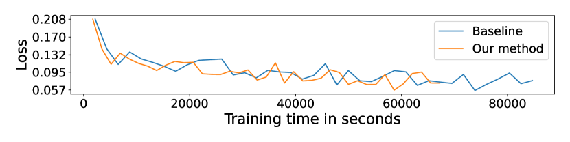
(a) VGG-16

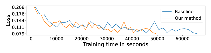
(b) DenseNet-121

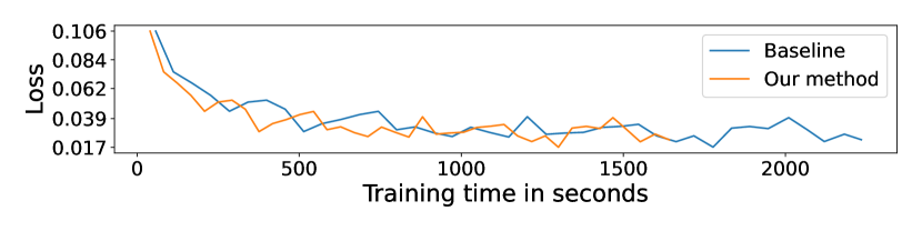
(c) AlexNet

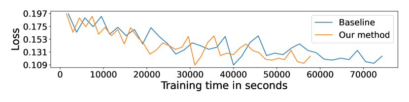
(d) EfficientNetB3

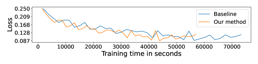
(e) Inception-V3

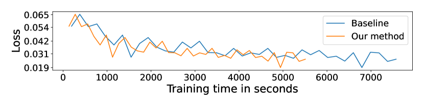
(f) ResNet-18

Figure 2: Training loss comparison of the proposed model w.r.t. the baseline, based on [13], for six different networks on CIFAR-10.

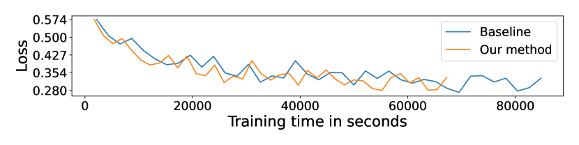
(a) VGG-16

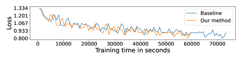
(b) DenseNet-121

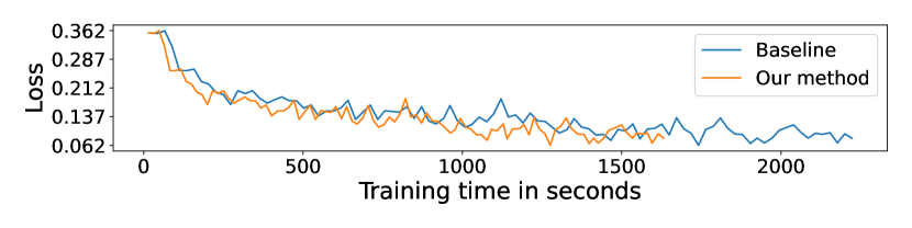
(c) AlexNet

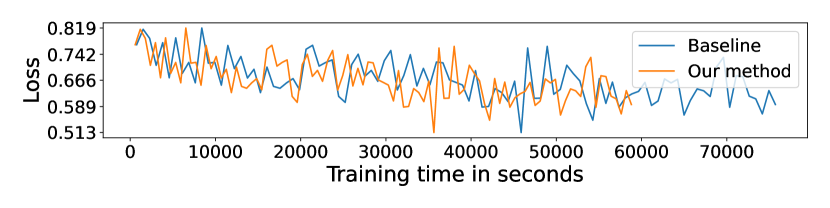
(d) EfficientNetB3

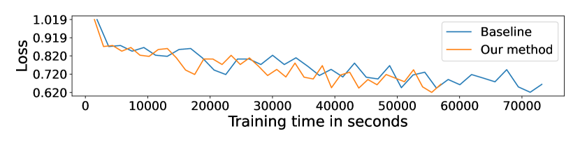
(e) Inception-V3

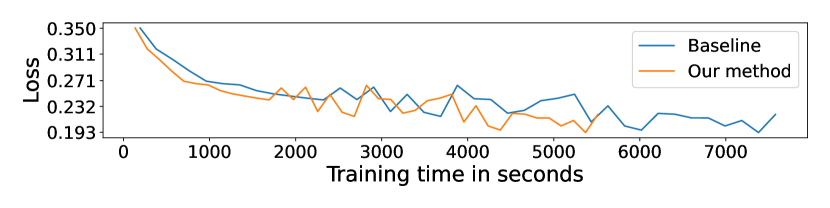
(f) ResNet-18

Figure 3: Training loss comparison of the proposed model w.r.t. the baseline, based on [13], for six different networks on CIFAR-100.

IV-G Additional Resources

The source code and output for the experimental results presented in this section are available online.

V Discussion

Traditionally, FFT-based CNN requires $4$ real-value multiplication and $2$ real-value additions to process each element of the convolution layer output in the spectral domain. Such cost is inherited from the complex multiplication cost of the rectangular form, (12), and it is approximated by $4Bf_{2}f_{1}N^{2}$ FLOPS in the original estimate of (1). Our method proposes using phasors to represent complex numbers as an alternative to the rectangular form. In this representation, the complex multiplication can be computed with only $1$ real-value multiplication and $1$ real-value addition, (13), yielding an estimate of $Bf_{2}f_{1}N^{2}$ FLOPS. Such reduction by $3/4$ in the number of FLOPS is reflected in the speedup presented in Tables I to Table IV, in which we observe that executions with larger batch sizes, $B$, tend to benefit more, which is expected given the FLOPS estimate.

In addition to Table III and Table IV, which show the final model performance in terms of loss and accuracy, Fig. 2 and Fig. 3 show that our method has equivalent performance to the baseline method. This is expected due to the nature of our method, which is mathematically equivalent to the baseline method, differing only due to the limitation of the numerical representation of float numbers. Compared to the baseline, our approach requires two extra steps, as shown in Fig. 1: Step#2 for computing (8) and (9); and Step#4 for calculating (10). Despite these additional steps, the experimental results show that our approach yields enough acceleration to compensate for those extra costs while significantly outperforming the baseline in all scenarios.

Note that Tables I to Table IV also shows that the higher the batch size, the larger the speedup gain, such characteristic is expected from (1). Though larger values are desirable, the batch size value is bound to the memory usage constraints. This trade-off of memory usage and speedup is not particular to our method but inherited from the adopted baseline.

Furthermore, our method can be combined with other approaches in the literature that focus only on reducing the cost of the FFT operations to yield even higher gains. Though the experimental results were obtained using GPU, our method is platform agnostic; hence, it can be easily translated to existing FFT-based CNNs used in embedded applications.

VI Conclusion

This paper investigates a phasor-based computational method to accelerate the training and inference speed of FFT-based CNNs. The proposed method benefits from the lower number of operations required by the phasor representation to multiply the Fourier representations of the inputs and kernels. The experimental analysis proves that our method outperforms the speed of the baseline method up to $1.376\times$ during training and up to $1.390\times$ during the inference while yielding similar accuracy.

Future research can be dedicated to further investigating the potential phasor representation with other types of implementation, such as using optimized CUDA kernels or targeting embedded platforms.

References

- [1] O. Russakovsky, J. Deng, H. Su, J. Krause, S. Satheesh, S. Ma, Z. Huang, A. Karpathy, A. Khosla, M. S. Bernstein, A. C. Berg, and L. Fei-Fei, “Imagenet large scale visual recognition challenge,” CoRR, vol. abs/1409.0575, 2014.
- [2] A. Krizhevsky, I. Sutskever, and G. E. Hinton, “Imagenet classification with deep convolutional neural networks,” in Advances in Neural Information Processing Systems 25: 26th Annual Conference on Neural Information Processing Systems 2012. Proceedings of a meeting held December 3-6, 2012, Lake Tahoe, Nevada, United States, 2012, pp. 1106–1114.
- [3] K. Simonyan and A. Zisserman, “Very deep convolutional networks for large-scale image recognition,” in 3rd International Conference on Learning Representations, ICLR 2015, San Diego, CA, USA, May 7-9, 2015, Conference Track Proceedings, Y. Bengio and Y. LeCun, Eds., 2015.
- [4] C. Szegedy, V. Vanhoucke, S. Ioffe, J. Shlens, and Z. Wojna, “Rethinking the inception architecture for computer vision,” in 2016 IEEE Conference on Computer Vision and Pattern Recognition, CVPR 2016, Las Vegas, NV, USA, June 27-30, 2016, 2016, pp. 2818–2826.
- [5] K. He, X. Zhang, S. Ren, and J. Sun, “Deep residual learning for image recognition,” in 2016 IEEE Conference on Computer Vision and Pattern Recognition, CVPR 2016, Las Vegas, NV, USA, June 27-30, 2016, 2016, pp. 770–778.
- [6] H. Zhu, M. Akrout, B. Zheng, A. Pelegris, A. Jayarajan, A. Phanishayee, B. Schroeder, and G. Pekhimenko, “Benchmarking and analyzing deep neural network training,” in 2018 IEEE International Symposium on Workload Characterization, IISWC 2018, Raleigh, NC, USA, September 30 - October 2, 2018, 2018, pp. 88–100.
- [7] Y. You, Z. Zhang, C. Hsieh, J. Demmel, and K. Keutzer, “Imagenet training in minutes,” in Proceedings of the 47th International Conference on Parallel Processing, ICPP 2018, Eugene, OR, USA, August 13-16, 2018, 2018, pp. 1:1–1:10.
- [8] H. Mikami, H. Suganuma, Y. Tanaka, Y. Kageyama et al., “Massively distributed sgd: Imagenet/resnet-50 training in a flash,” arXiv preprint arXiv:1811.05233, 2018.
- [9] M. Yamazaki, A. Kasagi, A. Tabuchi, T. Honda, M. Miwa, N. Fukumoto, T. Tabaru, A. Ike, and K. Nakashima, “Yet another accelerated SGD: resnet-50 training on imagenet in 74.7 seconds,” CoRR, vol. abs/1903.12650, 2019.
- [10] Q. Zhang, M. Zhang, T. Chen, Z. Sun, Y. Ma, and B. Yu, “Recent advances in convolutional neural network acceleration,” Neurocomputing, vol. 323, pp. 37–51, 2019.
- [11] “BLAS (basic linear algebra subprograms),” https://netlib.org/blas/, accessed: 2024-02-05.
- [12] A. Lavin and S. Gray, “Fast algorithms for convolutional neural networks,” in 2016 IEEE Conference on Computer Vision and Pattern Recognition, CVPR 2016, Las Vegas, NV, USA, June 27-30, 2016, 2016, pp. 4013–4021.
- [13] M. Mathieu, M. Henaff, and Y. LeCun, “Fast training of convolutional networks through ffts,” in 2nd International Conference on Learning Representations, ICLR 2014, Banff, AB, Canada, April 14-16, 2014, Conference Track Proceedings, 2014.
- [14] N. Vasilache, J. Johnson, M. Mathieu, S. Chintala, S. Piantino, and Y. LeCun, “Fast convolutional nets with fbfft: A GPU performance evaluation,” in 3rd International Conference on Learning Representations, ICLR 2015, San Diego, CA, USA, May 7-9, 2015, Conference Track Proceedings, 2015.
- [15] S. Chetlur, C. Woolley, P. Vandermersch, J. Cohen, J. Tran, B. Catanzaro, and E. Shelhamer, “cudnn: Efficient primitives for deep learning,” CoRR, vol. abs/1410.0759, 2014. [Online]. Available: http://arxiv.org/abs/1410.0759
- [16] A. Paszke, S. Gross, F. Massa, A. Lerer, J. Bradbury, G. Chanan, T. Killeen, Z. Lin, N. Gimelshein, L. Antiga, A. Desmaison, A. Köpf, E. Z. Yang, Z. DeVito, M. Raison, A. Tejani, S. Chilamkurthy, B. Steiner, L. Fang, J. Bai, and S. Chintala, “Pytorch: An imperative style, high-performance deep learning library,” in Advances in Neural Information Processing Systems 32: Annual Conference on Neural Information Processing Systems 2019, NeurIPS 2019, December 8-14, 2019, Vancouver, BC, Canada, 2019, pp. 8024–8035.
- [17] “Facebook’s cuda library,” https://github.com/facebookarchive/fbcuda, accessed: 2024-02-05.
- [18] T. Highlander and A. Rodriguez, “Very efficient training of convolutional neural networks using fast fourier transform and overlap-and-add,” in Proceedings of the British Machine Vision Conference 2015, BMVC 2015, Swansea, UK, September 7-10, 2015, 2015, pp. 160.1–160.9.
- [19] T. Abtahi, C. Shea, A. M. Kulkarni, and T. Mohsenin, “Accelerating convolutional neural network with FFT on embedded hardware,” IEEE Trans. Very Large Scale Integr. Syst., vol. 26, no. 9, pp. 1737–1749, 2018.
- [20] J. Lin and Y. Yao, “A fast algorithm for convolutional neural networks using tile-based fast fourier transforms,” Neural Process. Lett., vol. 50, no. 2, pp. 1951–1967, 2019.