StyDeSty: Min-Max Stylization and Destylization
for Single Domain Generalization

Abstract

Single domain generalization (single DG) aims at learning a robust model generalizable to unseen domains from only one training domain, making it a highly ambitious and challenging task. State-of-the-art approaches have mostly relied on data augmentations, such as adversarial perturbation and style enhancement, to synthesize new data and thus increase robustness. Nevertheless, they have largely overlooked the underlying coherence between the augmented domains, which in turn leads to inferior results in real-world scenarios. In this paper, we propose a simple yet effective scheme, termed as StyDeSty, to explicitly account for the alignment of the source and pseudo domains in the process of data augmentation, enabling them to interact with each other in a self-consistent manner and further giving rise to a latent domain with strong generalization power. The heart of StyDeSty lies in the interaction between a stylization module for generating novel stylized samples using the source domain, and a destylization module for transferring stylized and source samples to a latent domain to learn content-invariant features. The stylization and destylization modules work adversarially and reinforce each other. During inference, the destylization module transforms the input sample with an arbitrary style shift to the latent domain, in which the downstream tasks are carried out. Specifically, the location of the destylization layer within the backbone network is determined by a dedicated neural architecture search (NAS) strategy. We evaluate StyDeSty on multiple benchmarks and demonstrate that it yields encouraging results, outperforming the state of the art by up to 13.44% on classification accuracy. Codes are available here.

1 Introduction

Domain generalization (DG) (Wang et al., 2021a; Sinha et al., 2017; Volpi & Murino, 2019; Volpi et al., 2018) aims to tackle the distribution shift problem between source and target domain, and has recently demonstrated unprecedentedly promising results. The conventional setup of DG, as shown in Figure 1(a), includes multiple source domains $\mathbb{X}_{1},\mathbb{X}_{2},\cdots,\mathbb{X}_{N}$ during training and a novel domain during testing. As such, standard DG approaches have largely relied on learning a domain-invariant representation from the given domains, so that the model can be successfully generalized to other unseen domains. Nevertheless, access to data from multiple domains is, in reality, often infeasible due to data availability such as privacy and budgeting issues. This further calls for the single domain generalization (single DG) that handles the generation-learning task using only one source domain (Qiao et al., 2020).

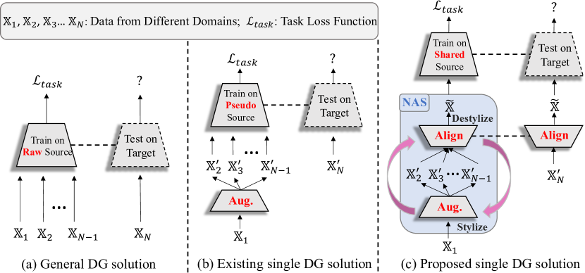
Figure 1: Workflows of general DG solution, existing single DG solution, and the proposed solution. (a) General DG methods are trained on multiple source domains to learn domain-invariant representations for generalization. (b) Existing single DG methods typically leverage data augmentation techniques to increase the domain diversity and then conduct training directly on the pseudo domains. (c) The proposed single DG solution enables an explicit stylization and destylization mechanisms to learn a latent domain, where the downstream tasks are performed. The stylization and destylization work in an adversarial fashion, and the location of destylization is determined by a NAS algorithm.

Unfortunately, off-the-shelf solutions to multi-domain DG are not applicable to single DG, since the former relies on domain identifiers as supervision signals for learning domain-invariant representation (Balaji et al., 2018; Chattopadhyay et al., 2020; Dou et al., 2019; Li et al., 2019), which are however not available in the latter. To address the more challenging single DG task, existing methods have resorted to data augmentation techniques to enhance the data diversity, including adversarial data pertubation (Qiao et al., 2020; Volpi et al., 2018) and style enhancement (Wang et al., 2021b; Zhou et al., 2020), as shown in Figure 1(b). Despite unprecedented advances, existing endeavors have focused on the generation of the augmented domains, yet largely overlooked the interconnections between such pseudo-domains and the source one, leading to the incompetent generalization capability and further inferior results, especially in the challenging in-the-wild scenarios.

In this paper, we introduce a novel single DG approach, termed as StyDeSty, to explicitly explore and take advantage of the underlying coherence between the source and augmented domains, in aim to learn a latent domain with strong generalization capability. The core idea of StyDeSty lies in that, samples from the pseudo-domains should share the same underlying distribution in a “hidden” domain, denoted as $\widetilde{\mathbb{X}}$, with the source. This hidden domain $\widetilde{\mathbb{X}}$, intuitively, resembles the content in style-transfer tasks; in other words, despite the diversified stylizations of $\mathbb{X^{\prime}}_{2},\mathbb{X^{\prime}}_{3},\cdots,\mathbb{X^{\prime}}_{N-1}$, their contents are all identical. Such domain-invariant content is, therefore, reasonably expected to be generalized well to unseen domains, which again can be treated as unknown stylizations upon the same content.

We show in Figure 1(c) the overall pipeline of the proposed StyDeSty. It comprises three key components: a stylization module, a destylization module, and a task head, in which the former two are optimized in a min-max game to reinforce each other. During training, the stylization module learns to generate novel stylized samples for the source domain, while the destylization learns to unify the features before and after stylization to an identical distribution in the latent domain, and explicitly enforces content consistency between features of style-augmented samples and original ones. During inference, testing samples, treated as unseen-stylized ones, are projected back to the learned latent domain, where the downstream tasks, such as classifications, are performed through the task-specific head.

Specifically, we first demonstrate the benefit of explicit destylization with an illustrating example. Then, we explore what is an appropriate objective to regulate the behavior of destylization, which provides insights for the adopted training algorithm. Finally, we reveal that the location of the key destylization layer is one crucial factor that affects the performance and devise a neural architecture search (NAS) strategy to automatically identify the optimal location. In other words, in this paper, we study and give solutions to three questions: why, how, and where to destyle in single DG? As demonstrated in our experiments, StyDeSty outperforms state-of-the-art models by $3.60\%$, $5.65\%$, and $13.44\%$ on Digits, CIFAR-10-C, and PACS respectively. Moreover, unlike previous DG techniques, StyDeSty does not require a specific label format like categorical data, which makes it a versatile solution for not only classification but also regression, such as depth estimation.

Our main contributions are thus summarized as follows:

• A novel single DG approach is introduced, termed as StyDeSty, to explicitly account for the alignment of the source and pseudo domains, achieved through an adversarial stylization and destylization game, where the two players reinforce each other.

• An effective objective is further proposed as supervision for the destylization module, along with the corresponding training strategy for the entire framework.

• A NAS approach is devised to identify the optimal location for destylization, which coordinates well stylizations, destylizations, and downstream tasks.

• The proposed StyDeSty serves as a versatile solution for universal supervised learning problems, applicable to not only classification but also regression tasks. Our method is evaluated extensively on multiple benchmarks and achieves superior performance.

2 Related Works

2.1 Alignment in General Domain Generalization

The key for generalization lies in learning domain-invariant representation so that different domains share a common feature/latent space (Ben-David et al., 2010). Thus, many methods rely on aligning the source domains by minimizing cross-domain feature difference (Motiian et al., 2017; Yu et al., 2023; Jin et al., 2020; Mahajan et al., 2021; Du et al., 2020; Yang et al., 2022a, b; Ye et al., 2023; Ye & Wang, 2024; Liu et al., 2022a; Muandet et al., 2013), e.g., based on distance metrics of maximum mean discrepancy (MMD) (Long et al., 2015; Yan et al., 2017), correlation distance (Sun & Saenko, 2016; Zhuo et al., 2017), and second-order moment (Peng et al., 2019; Jin et al., 2020). The other branch that achieves a similar goal tends to leverage the adversarial training strategy for generalization (Ganin & Lempitsky, 2015; Li et al., 2018b, a; Shao et al., 2019; Zhao et al., 2020b; Albuquerque et al., 2019). Although these methods could handle the general DG problem, they are still inapplicable to single DG where only one source domain is available since both of the distance minimization and adversarial training based DG methods need multiple source domains for optimization.

On the other routine, there are also works designing normalization mechanisms for feature alignment so that features from different domains share the same statistics. For example, (Seo et al., 2020) propose to learn the domain-specific batch normalization layer for each domain independently. (Fan et al., 2021) present an adversarial adaptive normalization where both the standardization and rescaling statistics are learned via neural networks instead of data-wise calculation. (Jin et al., 2021) design a restoration module that supplements the lost discriminative features due to the normalization operation. Differently, the feature destylization design in our paper is achieved by the adaptive instance normalization (AdaIN) (Huang & Belongie, 2017) which aims to transfer all the augmented and stylized features to the same distribution, so as to reach “alignment”. Moreover, destylization also enforces constraints to preserve content consistency before and after stylization, which further encourages the learning of style-/domain-invariant features.

We notice that (Yang et al., 2023) also adopt the AdaIN module for style alignment. Nevertheless, the augmentation techniques are limited to low-level transformations such as color jittering and Gaussian noise, resulting in relatively limited data diversity. Furthermore, their augmentation and alignment modules are trained independently. In contrast, the two modules learn mutually to reinforce each other in our method. We find that such an adversarial fashion impacts performance positively.

2.2 Single Domain Generalization

The problem of learning to generalize with only one available source domain can be tackled from different perspectives, such as projecting superficial statistics out (Wang et al., 2019b), penalizing local predictive power (Wang et al., 2019a), solving Jigsaw puzzles (Carlucci et al., 2019), clustering pseudo training domains (Matsuura & Harada, 2020), self challenging (Huang et al., 2020), meta architectures (Wan et al., 2022), attention consistency (Cugu et al., 2022), and debiasing and regularization (Qu et al., 2023).

However, recent data augmentation-based methods have achieved dominant performance for the single DG task by enriching the diversity of domain data. Representatively, (Volpi et al., 2018) propose to apply adversarial perturbations into the source samples to augment domain data. (Zhao et al., 2020a) further add regularization to adversarial perturbations via maximum entropy. (Li et al., 2021) and (Kang et al., 2022) propose to generate novel styles progressively and constantly. (Cheng et al., 2023) propose Beyasian augmentation. (Lv et al., 2022) and (Chen et al., 2023) augment data by leveraging causal knowledge. (Qiao et al., 2020) make the learning with adversarial data augmentation become learnable and optimize it in a bi-level meta-learning framework. Similar ideas are also explored in (Fu et al., 2023), (Chen et al., 2022), and (Zhong et al., 2022). Beyond adversarial perturbations, many recent data augmentation-based single DG methods tend to use style transfer techniques for domain enlargement, e.g., (Zhou et al., 2020) train an image-to-image generator for each source domain to synthesize novel domains, (Zhou et al., 2021) mix up the styles of source images to generate new domain data, (Wang et al., 2021b) propose a style complement module to increase the diversity of domain data, (Choi et al., 2023) propose progressive random convolution for style augmentation, and (Zhao et al., 2022) utilize farthest point sampling to select style vectors for style augmentation. However, these methods over-explore the domain augmentation (i.e., stylization) but ignore the important effect of the explicit feature alignment and the underlying coherence among augmented domains w.r.t model generalization, which makes the trained model hard to be generalized to test domains with unseen styles in inference. This drawback motivates us to further consider unifying/aligning the distribution of augmented domains by destylization and thus increase model robustness against style variance. How to balance such two designs of stylization and destylization is also the focus of this paper.

3 Methodology

The heart of the StyDeSty framework is at the interaction of its three components: a stylization module $G$, a destylization module $F$, and a task head $H$. An overview of our method is illustrated in Figure 2. We start the introduction of the key stylization and destylization modules first and then elaborate on the training objective. Finally, a NAS-guided training algorithm is proposed, which coordinates the interaction between stylization and destylization, and regulates the whole StyDeSty pipeline.

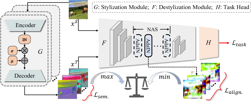
Figure 2: StyDeSty framework consists of a stylization module $G$, a destyliation module $F$, and a task head $H$, where a NAS algorithm is involved to search an optimal position of the AdaIN layer for destylization. Black and red arrows denote forward pass and loss computation and IN represents instance normalization.

3.1 Stylization and Destylization

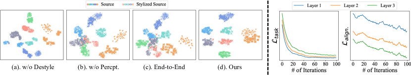
Figure 3: Left: TSNE visualizations of stylized and original source samples for by different fashions of destylization. Right: Visualizations of task loss and alignment loss with destylization at different locations in a deep network.

Stylization Module. Similar to style transfer (Gatys et al., 2016; Huang & Belongie, 2017; Liu et al., 2021a, 2022b, 2020, 2023; Tang et al., 2023), the stylization module $G$ aims to generate various stylized versions given a source image $x^{\mathcal{S}}$ from a source domain $\mathcal{S}$. In this paper, similar to the style complement module in (Wang et al., 2021b), $G$ consists of $B$ blocks, with a single convolution layer $enc_{j}$, an instance normalization layer, an affine transformation layer parameterized by $\mu_{j}$ and $\sigma_{j}$, and a symmetric deconvolution layer $dec_{j}$ for the $j$-th block, $1\leq j\leq B$. Given an input RGB image $x^{\mathcal{S}}$, the $j$-th block firstly projects it to a $c$-dimension feature space with $enc_{j}$ to derive $f_{j}\in\mathbb{R}^{h\times w\times c}$. Then, the instance normalization layer normalizes $f_{j}$ with the channel-independent mean $\mu^{f}_{j}$ and standard deviation $\sigma^{f}_{j}$, followed by the affine transformation layer to get $\hat{f_{j}}$. At last, $dec_{j}$ projects $\hat{f_{j}}$ back to the RGB space, and the result is denoted as $\hat{x_{j}}$. Formally, this process can be written as:

$$f_{j}={\rm enc}_{j}(x^{\mathcal{S}}),\hskip 2.84526pt\hat{f_{j}}=\sigma_{j}\times\frac{f_{j}-\mu^{f}_{j}}{\sigma^{f}_{j}}+\mu_{j},\hskip 2.84526pt\hat{x_{j}}={\rm dec}_{j}(\hat{f_{j}}).$$ (1)

Notably, the affine parameters $\mu_{j}$ and $\sigma_{j}$ for some blocks have shape $h\times w\times c$ while the other ones are with shape $1\times 1\times c$, to mimic local and global distortions respectively. The final augmented result $x^{\mathcal{T}}$ is given as a weighted sum of the outputs of all the $B$ blocks, with the weight vector $w\in\mathbb{R}^{B}$ drawn from a standard normal distribution in each training iteration:

$$w\sim\mathcal{N}(0,1),\hskip 8.53581ptx^{\mathcal{T}}={\rm sigmoid}(\frac{1}{\sum_{j=1}^{B}w_{j}}w_{j}\hat{x_{j}}),$$ (2)

where the ${\rm sigmoid}$ is applied to scale the augmented images.

Destylization Module. The destylization module $F$ is typically composed of the first several blocks of a backbone network and a destylization layer. For example, for the classification problem, if ResNet-18 (He et al., 2016) with $4$ main blocks is selected as the backbone network, we can take the former $2$ blocks to build the destylization module and the remaining parts would serve as the task head $H$. The core of the destylization module is the final destylization layer accounting for underlying coherence and explicitly distribution aligning. In this paper, we adopt adaptive instance normalization (AdaIN) (Huang & Belongie, 2017), a simple but effective mechanism in arbitrary style transfer, for instantiation. The insight is that channel-wise statistic information like mean and variance in a deep network can largely represent the style of an image. In this sense, the alignment of these statistics can be viewed as transferring all the images to the same style/latent, which is known as destylization in this paper. The unified style is encoded by the affine parameters of the AdaIN layer and the formulation is similar to that of the stylization module:

$${\rm AdaIN}(f,\mu,\sigma)=\sigma\times\frac{f-\mu^{f}}{\sigma^{f}}+\mu,$$ (3)

where $\mu$ and $\sigma$ are learnable affine parameters while $\mu^{f}$ and $\sigma^{f}$ are the channel-wise mean and standard deviation of a feature map $f$ produced by the layer before AdaIN.

Discussion: Why to Destyle? We provide an illustrating example in Figure 3(left) to demonstrate how our destylization module works. We conduct training on the photo domain of PACS dataset (Li et al., 2017) and visualize the learned representation of each sample using TSNE (Van der Maaten & Hinton, 2008), where the different classes are denoted by different colors, and the original source samples and stylized ones are denoted by different markers. As shown in the plot (a), although the previous methods like L2D (Wang et al., 2021b) have used style augmentation to increase diversity, they still suffer from the domain shift problem given unseen styles in inference without a kind of explicit alignment/destylization. In contrast, with an explicit destylization operation, our method largely alleviates such a problem (see plot (d)), which means better robustness to style shifts. More results can be found in the supplementary.

3.2 Objective Functions

The overall loss function is inspired by (1) the recent works on adversarial data augmentation (Sinha et al., 2017; Qiao et al., 2020; Zhao et al., 2020a), and (2) the classic theory of domain adaptation (Ben-David et al., 2010) – the test error is largely dominated by the source training risk and the discrepancy between the source and target domain:

$$\min\sup_{\mathcal{T}=G(\mathcal{S}):W(\mathcal{S},\mathcal{T})\leq\rho}\mathbb{E}_{\mathcal{T}}[ \mathcal{L}_{task}(H(F(x^{\mathcal{T}})),y^{\mathcal{T}})$$ (4)

$$+\alpha \mathcal{L}_{align.}(F(x^{\mathcal{S}}),F(x^{\mathcal{T}}))],$$

where $\mathcal{T}$ denotes synthetic target domains by data augmentation, $x^{\mathcal{T}}\sim\mathcal{T}$ is an instance sampled from $\mathcal{T}$ and augmented from the source sample $x^{\mathcal{S}}\sim\mathcal{S}$, $G$ and $F$ are instantiated as the stylization and destylization modules respectively in this paper, $\mathcal{L}_{align.}$ is a metric of alignment between two features, $\alpha$ is a hyperparameter controlling the weight of this constraint, and $\rho$ is another hyperparameter denoting the maximal strength of data augmentation. Since it is intractable for deep networks to solve the constrained optimization problem in Equation 4, we alternatively consider the following objective by Lagrangian relaxation:

$$\min\sup_{\mathcal{T}=G(\mathcal{S})}\{\mathbb{E}_{\mathcal{T}}[ \mathcal{L}_{task}(H(F(x^{\mathcal{T}})),y^{\mathcal{T}})$$ (5)

$$+\alpha\mathcal{L}_{align.} (F(x^{\mathcal{S}}),F(x^{\mathcal{T}}))]-\beta W(\mathcal{S},\mathcal{T})\},$$

where $\beta\geq 0$ is a penalty factor with an intuitive meaning similar to $\rho$. Equation 5 offers insights into the loss functions of each component which will be illustrated below.

Task head. The task head $H$ in the StyDeSty framework aims to discriminate information related to the task from the unified distribution/latent by the destylization module $F$. Through Equation 5, we can find that the feature alignment metric $\mathcal{L}_{align.}$ and the W-distance term are not related to $H$. Therefore, $H$ is trained with only the task-specific loss $\mathcal{L}_{task}(H(F(x^{\mathcal{T}})),y^{\mathcal{T}})$. Notably, StyDeSty is a versatile framework applicable for different tasks with different forms of $\mathcal{L}_{task}$. For instance, in classification problems, cross-entropy loss is a typical option, while in regression problems, we can use $L1$ or $L2$ loss as $\mathcal{L}_{task}$.

Destylization Module: How to Destyle. As suggested by Equation 5, there are two components for the objective of the destylization module $F$: task-specific loss $\mathcal{L}_{task}$ and feature alignment metric $\mathcal{L}_{align.}$. The configuration of $\mathcal{L}_{task}$ is the same as that in the task head. As for the feature alignment term, one straight-forward idea is to measure the Euclidean distance or $L2$ distance between the two feature maps $F(x^{\mathcal{S}})$ and $F(x^{\mathcal{T}})$. However, as shown in the plot (b) of Figure 3, we find that this configuration often leads to inferior results. One major problem is that not all positions and channels are worth aligning equally for the current task. To increase the awareness of key features for this distance metric, we further adopt the task head as a perceptual network and measure the feature distance at the last hidden layer of $H$, denoted as $H_{-1}$. In this way, we have the following loss function for the destylization module:

$$\mathcal{L}_{align.} (F(x^{\mathcal{S}}),F(x^{\mathcal{T}}))=\|F(x^{\mathcal{S}})-F(x^{\mathcal{T}})\|^{2}$$ (6)

$$+\lambda \|H_{-1}(F(x^{\mathcal{S}}))-H_{-1}(F(x^{\mathcal{T}}))\|^{2},$$

$$\mathcal{L}_{F}= \frac{1}{n}\sum_{i=1}^{n}\{\mathcal{L}_{task}(H(F(x_{i}^{\mathcal{T}})),y_{i}^{\mathcal{T}})$$

$$+\alpha\mathcal{L}_{align.}(F(x_{i}^{\mathcal{S}}),F(x_{i}^{\mathcal{T}}))\},$$

where $\lambda$ is a hyper-parameter balancing the weight of the perceptual term and $n$ is the size of a mini-batch.

It is worth noting that the task head $H$ serves as a metric function here and its parameters should not be updated according to the gradient of $\mathcal{L}_{align.}$. Therefore, we do not train modules $G$ and $H$ simultaneously but update them alternately. Otherwise, the task head would also help alignment, which weakens the alignment ability of the destylization module, as demonstrated in the plot (c) of Figure 3.

Stylization Module. The stylization module $G$ behaves adversarially against $F$ and $H$. Moreover, it is not allowed to destroy the semantics of the original images to generate meaningless stylized results. Therefore, we introduce a semantic perceptron $M$ to enforce the semantic consistency constraint $\mathcal{L}_{sem.}$ on $G$. Besides, the time complexity of solving the W distance as indicated by Equation 5 for a batch of data is considerable for an iterative algorithm. We then alternatively consider the dual form of the W distance, which is equivalent to the maximum mean discrepancy (MMD) with a Lipschitz continuous kernel function $k$ under some mild conditions (Edwards, 2011). In this sense, the loss function for $G$ can be written as:

$$\mathcal{L}_{sem.}=\|\frac{1}{n}\sum_{i=1}^{n}k(M(x^{\mathcal{S}}_{i})) -\frac{1}{n}\sum_{i=1}^{n}k(M(x^{\mathcal{T}}_{i}))\|^{2},$$ (7)

$$\mathcal{L}_{G}=-\mathcal{L}_{F} +\beta\mathcal{L}_{sem.}.$$

3.3 Training with NAS: Where to Destyle

With the different objective functions for each module, the training process can be organized as a three-stage algorithm, to train $F$, $H$, and $G$ alternately in each iteration. Nevertheless, we have to answer an important question before the formal training: how to select an appropriate position in a backbone network to insert the destylization layer and split the network into $F$ and $H$? Empirically, we observe that there is a trade-off between the objectives of the task ahead and the alignment. As demonstrated in Figure 3(right), the deeper destylization could benefit the alignment of the source and stylized samples but make the task head training difficult, since it is more convenient to enforce the features with high-level semantics to be aligned by discarding discriminative information. In this paper, instead of selecting the position heuristically, we devise a neural architecture search (NAS) strategy to address this problem. Assume that there is a backbone network $P$ with $L$ positions that are potentially suitable for inserting the AdaIN layer which splits $P$ into $L+1$ blocks with the $l$-th one denoted as $p_{l}$. In the NAS stage, we insert AdaIN layers, denoted as ${\rm AdaIN}_{l}$ with $1\leq l\leq L$, to all the $L$ positions and optimize a vector $\pi\in\mathbb{R}^{L}$, where $\pi_{l}$ indicates the logit value that the $l$-th AdaIN layer is enabled. We denote the output of the $l$-th block as $x_{l}$, and $x_{l}$ for $1\leq l\leq L$ is given by:

$$\hat{\pi}={\rm GumbelSoftmax} (\pi),\hskip 8.53581pt\hat{x_{l}}=p_{l}(x_{l-1}),$$ (8)

$$x_{l}=\hat{\pi_{l}}{\rm AdaIN}_{l} (\hat{x_{l}})+(1-\hat{\pi_{l}})\hat{x_{l}}.$$

Here, the Gumbel-Softmax function (Jang et al., 2016) is applied on $\pi$, which would produce a one-hot vector $\hat{\pi}$ indicating the selected AdaIN layer in this iteration.

Algorithm 1 Training of StyDeSty

Required: A source domain $\mathcal{S}$; A randomly-initialized stylization module $G$; A randomly initialized backbone $P$ with $L$ candidate AdaIN layers; A zero initialized vector $\pi$ for selecting the enabled AdaIN.

1:  repeat

2:     Train $P$ and $\pi$ by Equation 9 for $T_{P}$ times;

3:     Train $G$ by Equation 10 for $T_{G}$ times;

4:  until $\operatorname*{arg\,max}\pi$ does not change{NAS Stage}

5:  Select the AdaIN layer $l$ with maximal $\pi_{l}$ and split $P$ into $F$ and $H$;

6:  repeat

7:     Train $F$ by Equation 6 for $T_{F}$ times;

8:     Train $H$ by $\mathcal{L}_{task}$ for $T_{H}$ times;

9:     Train $G$ by Equation 7 for $T_{G}$ times;

10:  until convergence{Formal training stage}

For optimization, all the parameters of $P$ including $\pi$ are updated together in the NAS time since the split position for the destylization module and the task head is unknown. $P$ and $G$ are still trained in a min-max game and their loss functions are formulated as:

$$\mathcal{L}_{P}=\frac{1}{n}\sum_{i=1}^{n}\{ \mathcal{L}_{task}(P(x_{i}^{\mathcal{T}}),y_{i}^{\mathcal{T}})$$ (9)

$$+\alpha\sum_{l=1}^{L}\hat{\pi_{l}}\|{\rm AdaIN}_{l} (\hat{x^{\mathcal{S}}_{i,l}})-{\rm AdaIN}_{l}(\hat{x^{\mathcal{T}}_{i,l}})\|^{2}\},$$

$$\mathcal{L}_{G}=-\mathcal{L}_{P}+\beta\mathcal{L}_{sem.}.$$ (10)

Note that here we do not incorporate the perceptual term in Equation 6 which requires passing through features after each ${\rm AdaIN}_{l}$ till the last layer and increases the computational burden significantly. The NAS procedure will repeat until the selected index of AdaIN layer does not change in further iterations. The overall training is summarized as Algorithm 1. The memory complexity and time complexity per iteration are consistent with those augmentation-based DG methods like L2D (Wang et al., 2021b), while the overall time complexity is related to $T_{P}$, $T_{G}$, $T_{F}$, and $T_{H}$.

4 Experiments

4.1 Datasets

To demonstrate the effectiveness and versatility of the proposed StyDeSty for single DG, we conduct extensive evaluations on three classification benchmarks: Digits, CIFAR-10-C, and PACS, and one regression problem: monocular depth estimation on the KITTI and vKITTI dataset. More comparisons can be found in the appendix.

Digits. Digits consists of $5$ digit recognition datasets including MNIST (LeCun et al., 1998), SVHN (Netzer et al., 2011), MNIST-M (Ganin & Lempitsky, 2015), SYN (Ganin & Lempitsky, 2015), and USPS (Denker et al., 1988), with variance on foreground shapes and background patterns. MNIST is used as the source domain containing 60,000 training images. We convert all the images to $32\times 32$ resolution with RGB format in the experiment.

CIFAR-10-C. CIFAR-10-C dataset (Hendrycks & Dietterich, 2019) is the corrupted version from the original CIFAR-10 (Krizhevsky et al., 2009) dataset, including 10 classes and totally 50,000 training images with $32\times 32$ resolution. There are 4 categories of corruption including weather, blur, noise, and digital. For each category, the corruption level is marked from 1 (mildest) to 5 (severest).

Method	SVHN	M-MNIST	SYN	USPS	Avg.
Source Only	27.83	52.72	39.65	76.94	49.29
JiGen	33.80	57.80	43.79	77.15	53.14
RSC	31.04	46.62	34.81	64.42	44.22
MMLD	26.41	51.51	38.33	75.04	47.82
ADA	35.51	60.41	45.32	77.26	54.62
M-ADA	42.55	67.94	48.95	78.53	59.49
ME-ADA	42.56	63.27	50.39	81.04	59.32
MixStyle	32.29	53.48	42.35	81.17	52.32
L2D	62.86	87.30	63.72	83.97	74.46
Ours	67.48	90.75	69.40	87.64	78.82

Table 1: Comparisons of single DG accuracy (%) on Digits. MNIST is used for training while the others are for evaluation.

PACS. PACS dataset (Li et al., 2017) contains 9,991 images of 4 domains: photo, art painting, cartoon, and sketch with 7 classes. The cross-domain variance in style and deformation is considerable and the adopted resolution is $224\times 224$, which makes it a more challenging benchmark.

KITTI and vKITTI: KITTI (Geiger et al., 2013) is an outdoor dataset with 42,382 images for automatic driving. In this paper, we use the test dataset for evaluation. The training domain is vKITTI dataset (Gaidon et al., 2016) containing 21,260 frames with depth labels from the Unity game engine. All the images are resized to $640\times 192$ resolution for training and evaluation.

Settings		Source Only	JiGen	RSC	MMLD	ADA	ME-ADA	MixStyle	L2D	Ours
Photo	Art	62.26	60.74	67.72	64.59	64.31	65.62	67.42	68.07	72.12
	Cartoon	27.60	33.40	33.70	30.25	34.94	36.95	36.34	34.43	55.03
	Sketch	29.35	43.96	48.00	28.61	36.12	35.10	38.28	44.69	62.61
	Avg.	39.73	46.03	49.81	41.15	45.12	45.89	47.35	49.06	63.25
Art	Photo	96.29	96.71	92.75	96.47	95.81	95.69	97.23	96.11	94.13
	Cartoon	61.01	58.40	71.89	55.97	67.96	67.28	64.66	70.61	71.97
	Sketch	49.25	51.23	69.43	41.46	68.26	65.31	54.32	65.08	74.09
	Avg.	68.85	68.78	78.02	64.63	77.34	76.09	72.07	77.26	80.06
Cartoon	Photo	85.27	85.57	85.33	85.33	85.99	84.49	87.72	86.17	87.78
	Art	63.38	68.90	71.00	62.11	68.55	57.82	71.59	75.24	75.93
	Sketch	67.73	63.35	73.30	66.07	72.28	71.82	63.78	73.40	75.87
	Avg.	72.13	72.60	76.54	71.17	75.61	74.71	74.36	78.27	79.86
Sketch	Photo	24.73	36.65	44.25	21.13	25.33	26.53	27.10	48.63	58.80
	Art	22.61	28.61	52.00	18.36	27.88	28.61	26.20	48.38	60.11
	Cartoon	41.13	41.30	61.86	34.04	58.70	52.89	52.07	62.88	67.75
	Avg.	29.49	35.51	52.70	24.51	37.30	36.01	35.12	53.40	62.22
Avg.		52.55	55.73	64.27	50.37	58.84	58.18	57.23	64.50	71.35

Table 2: Comparisons of single DG accuracy (%) on the PACS dataset. The first column indicates the training domain while the second column indicates the unseen test domain. Results under the ResNet-18 backbone are reported. Best performances in comparisons are highlighted in bold and the second best ones are marked with underlines.

4.2 Comparison with Sate-of-the-arts

We mainly compare StyDeSty with 8 state-of-the-art single DG methods, including Jiasaw-puzzle based JiGen (Carlucci et al., 2019), self-challenging based RSC (Huang et al., 2020), clustering based MMLD (Matsuura & Harada, 2020), adversarial augmentation based ADA (Volpi et al., 2018), M-ADA (Qiao et al., 2020), ME-ADA (Zhao et al., 2020a), and style enhancement based MixStyle (Zhou et al., 2021) and L2D (Wang et al., 2021b), as well as the Source Only baseline. All the comparisons are conducted using the same datasets and backbone networks. For our method, by default, the batch size is set as $64$ and the optimizer is SGD. The optimizer for $F$ and $H$ uses a $0.0005$ weight decay and $0.9$ momentum with the Nesterov mode (Nesterov, 1983). Learning rates for $F$, $H$, and $G$ are $0.001$, $0.001$, and $0.005$. The times of inner iteration in Algorithm 1 are all $1$ except that $T_{H}$ is $10$. The hyper parameters $\alpha$, $\lambda$, and $\beta$ are $0.1$, $1$, and $1$ respectively. As for the semantic perceptual network $M$ in Equation 7 and Equation 10, we directly use the task head $H$ itself as $M$ for all the classification tasks and features of the last hidden layer are adopted for $\mathcal{L}_{sem.}$. For the depth estimation problem, we load a fixed VGG19 model (Simonyan & Zisserman, 2014) pretrained on ImageNet (Russakovsky et al., 2015) as $M$ and $\mathcal{L}_{sem.}$ would use features of the ReLU-4_1 layer.

Method	Art	Cartoon	Sketch	Avg.
w/o Style	66.89	41.64	37.06	48.53
AutoAug	70.80	44.50	50.09	55.13
DCGAN	73.54	47.01	49.50	56.68
w/o Destyle	69.68	41.42	41.33	50.81
Separate Style Transfer	70.51	53.33	58.39	60.74
w/o $\mathcal{L}_{align.}$	72.51	49.70	56.20	59.47
w/o $Percpt.$	69.53	47.35	52.25	56.38
end-to-end	68.85	45.65	55.41	56.63
w/o Adv.	71.58	53.63	59.63	61.61
Ours	72.12	55.03	62.61	63.25

Table 3: Ablation studies of single DG accuracy (%) on PACS dataset. The photo domain is used for the training domain while the other three are for evaluation.

Comparisons on Digits. On the Digits dataset, we follow previous works and adopt the 5-layer LeNet (LeCun et al., 1998) as the backbone. There are 6 candidate positions to insert the AdaIN layer which are positions after the first and second convolution layer, ReLU layer, and pooling layer. NAS selects the position after the first pooling layer.

The model is trained on the MNIST and evaluated on the other four. Comparisons of results by different methods are shown in Tab. 1. The improvement over the state-of-the-art methods is consistent: $4.62\%$, $3.45\%$, $5.68\%$, and $3.67\%$ on the 4 test datasets, which outperforms the state-of-the-art method L2D (Wang et al., 2021b) by $4.36\%$ in average.

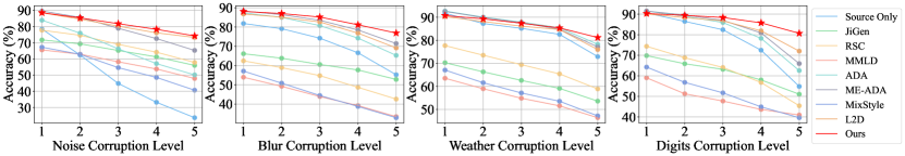
Figure 4: Relationships between accuracy results and corruption levels of four categories on CIFAR-10-C dataset. Our method demonstrates more robustness compared with other methods as the corruption increases.

Method	Photo	Art	Cartoon	Sketch	Avg.
Source Only	96.05	75.68	74.02	69.87	78.91
JiGen	96.47	80.62	74.71	72.43	81.06
RSC	93.95	82.81	79.74	83.51	85.00
MMLD	96.33	82.81	78.33	75.29	83.19
ADA	95.63	82.81	78.33	75.29	83.02
ME-ADA	95.33	77.88	78.58	78.07	82.47
MixStyle	96.31	83.11	79.43	72.95	82.95
L2D	95.15	83.69	80.16	82.01	85.25
Ours	95.27	84.03	79.86	82.23	85.35

Table 4: Comparisons of leave-one-domain-out classification accuracy (%) on PACS using ResNet-18 backbone. The column name indicates the test domain and the other three are used for training.

Comparisons on CIFAR-10-C. Following the common setting, we adopt WideResNet (16-4) (Zagoruyko & Komodakis, 2016) as the backbone for the CIFAR-10-C dataset. There is one convolution layer followed by three residual blocks for this backbone, which means that the number of candidate positions for the AdaIN layer is 4. The optimal position indicated by the NAS algorithm is after the first residual block. The batch size used is $128$ and learning rates for $F$, $H$, and $G$ are $0.1$, $0.1$, and $0.001$ respectively.

In this experiment, the original CIFAR-10 dataset is used as the training domain and the corrupted images are used for evaluation. The accuracy results w.r.t the corruption level for each method are plotted as Figure 4, which demonstrates that the model by our method can resist image corruption most robustly. On the severest corruption level 5, our method outperforms others by $0.94\%$, $5.46\%$, $2.96\%$, and $8.67\%$ for the four corruption categories respectively, and makes an average improvement of $5.65\%$.

Comparisons on PACS. We adopt ResNet-18 (He et al., 2016) backbone on the PACS dataset. As a convention, a pre-trained checkpoint on ImageNet dataset (Russakovsky et al., 2015) is loaded for initialization. We consider positions after the 4 main blocks as candidate AdaIN positions and the solution by the NAS algorithm is after the 2nd block.

Following previous arts, the results of using each of the four domains for training respectively, and the other three for evaluation are reported in Tab. 2. In almost all cases, our method performs significantly better than previous state-of-the-art ones, especially for scenarios where the domain shift is dramatic, like $14.61\%$ improvement when generalizing from the photo to the sketch domain. On average, our method outperforms others by $13.44\%$ when using the photo domain for training and $6.85\%$ overall by averaging the four training domains. Readers can refer to the supplementary material for results of more different architectures of backbone networks.

We also conduct experiments under the leave-one-out setting of general DG, to use three domains for training and the remaining one for evaluation, by mixing the data of three domains as one domain. ResNet-18 is used as the backbone and the selected AdaIN positions are all between the 1st and 2nd residual blocks in the 4 cases. Results in Tab. 4 prove that our method can produce at least comparable performance without any constraint on label space, which indicates the versatility of the proposed method.

Method	Photo	Art	Cartoon	Sketch	Avg.
Ours	63.25	80.06	79.86	62.22	71.35
(Lv et al., 2022)	46.21	75.64	78.29	58.44	64.65
(Lv et al., 2022)+Ours	54.36	79.33	78.99	60.77	68.36
(Chen et al., 2023)	57.99	76.18	77.91	58.11	67.55
(Chen et al., 2023)+Ours	64.36	78.46	79.62	59.63	70.52
(Choi et al., 2023)	62.89	76.98	78.54	57.11	68.88
(Choi et al., 2023)+Ours	67.98	81.82	80.80	63.15	73.44

Table 5: Single DG accuracy (%) on PACS dataset when our method is built on state-of-the-art ones as a plug-and-play component. The column name indicates the training domain, and the other three are used for training. The average performance over the three test domains is reported.

Comparisons on KITTI: In addition to the above classification tasks, we conduct experiments on a regression problem: monocular depth estimation on the KITTI dataset. The backbone network is a 4-level UNet-like (Ronneberger et al., 2015) architecture following  (Zhao et al., 2019). For our method, we insert AdaIN layers to the upper three skip connection structures as well as the bottom level. Adam (Kingma & Ba, 2014) is used as the optimizer with a learning rate of $0.0001$.

In this part, we mainly compare StyDeSty in this paper with those methods without constrain on the label space, including MixStyle (Zhou et al., 2021) and a variant of L2D (Wang et al., 2021b) by removing the class-conditional terms that are incompatible with this task, denoted as v-L2D. Using vKITTI as the source domain, evaluation results on the test KITTI dataset are shown in Tab. 6. Through all the metrics, we can observe that our method generalizes to the unseen target domain best by learning style-invariant feature representations, which demonstrates the versatility and superiority of StyDeSty.

4.3 Empirical Analysis

Method	Higher is better			Lower is better
	$\delta<1.25$	$\delta<1.25^{2}$	$\delta<1.25^{3}$	Abs Rel	Squa Rel	RMSE	$\rm{RMSE}_{log}$
Source Only	0.642	0.861	0.944	0.236	2.171	7.063	0.315
MixStyle	0.701	0.887	0.952	0.216	2.155	6.895	0.291
v-L2D	0.708	0.892	0.954	0.211	2.103	6.794	0.291
Ours	0.739	0.905	0.958	0.197	2.054	6.684	0.276

Table 6: Comparisons of monocular depth estimation on KITTI dataset. The vKITTI dataset extracted from a game engine is used for the training domain and the KITTI test dataset is for evaluation. Best performances in comparisons are highlighted in bold and the second best ones are marked with underlines.

Ablation Study. To validate the effectiveness of some key designs in our StyDeSty framework, we conduct ablations on the PACS dataset as shown in Tab. 3. We first study the effect of the stylization module, which intuitively diversifies the source domain and tells the model what information can be potentially variable in the inference time. Without this module, the model is unaware of domain-invariant features, leading to the misalignment of features that should remain distinct. As shown in the first three settings of Tab. 3, we try both removing the data augmentation module and replacing it with augmentations other than the stylization in this paper, like the widely used AutoAug (Cubuk et al., 2018) a vanilla DCGAN (Radford et al., 2016) generator. The results are measured on PACS taking Photo as the training domain and the remaining ones as test domains. Their inferior performance compared with the default setting of StyDeSty verifies the effectiveness of the stylization module.

Then, we delete the AdaIN layer for destylization (w/o Destyle) and find that the performance would drop significantly, which demonstrates that explicit feature alignment contributes to the generalization ability a lot. We also try replacing the destylization module with a pre-trained style transfer module (Huang & Belongie, 2017), which is unaware of the downstream task. The performance gap indicates the effectiveness of the task-aware destylization in our method. Plus, only aligning the second-order statistics does not make the model aware of invariant features without the metric $\mathcal{L}_{align.}$ in Equation 6(w/o $\mathcal{L}_{align.}$) and the model would produce inferior performance compared with that of the full model. Moreover, if only the $L2$ loss between normalized features is considered in $\mathcal{L}_{align.}$ without the perceptual term (w/o $Percpt.$), the performance can become even worse. However, it is non-trivial to add the perceptual term in the task-specific feature space of $H_{-1}$. If the network is trained in an end-to-end manner with $F$ and $H$ being updated at the same time (end-to-end), which means that the task head would also be affected by the perceptual alignment loss, the ability of the destylization module to learn a unified distribution would be weakened and the performance is also unsatisfactory. That is why StyDeSty uses a multi-stage training strategy and achieves the best performance, which drives both explicit distribution alignment and an appropriate constraint on aligned features.

We finally make the stylization module a random style augmenter in each iteration instead of playing against the destylization module adversarially. The performance drop demonstrates the effectiveness of their interplay.

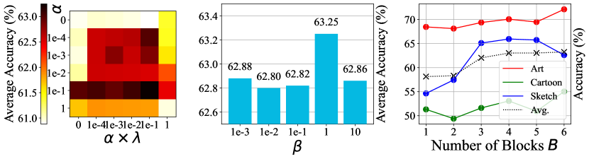
Figure 5: Sensitivity analysis for loss weights: $\alpha$, $\beta$, $\lambda$, and $B$.

Complementarity with Other Methods. The destylization mechanism can also serve as a plug-and-play component to improve the performance of other state-of-the-art methods. We apply the destylization layer and the corresponding position found by the NAS algorithm to the backbones of (Lv et al., 2022), (Chen et al., 2023), and (Choi et al., 2023), respectively. The results on PACS are shown in Tab. 5, where the single DG results are shown. The column name indicates the training domain, and the other three are used for training. We report the average performance over the three test domains. The results indicate that our method can improve other single DG methods as a general enhancer. When applied on (Choi et al., 2023), it achieves even better performance than the original StyDeSty framework in the default setting of this paper.

Sensitivity Study for Hyper-parameters. We conduct analysis for loss weights: $\alpha$, $\beta$, and $\lambda$ on the PACS dataset. As shown in Equation 6, the overall weights of the $L2$ distance and the perceptual term are $\alpha$ and $\alpha\times\lambda$ respectively, whose sensitivity is analyzed in Figure 5(left). The sensitivity of $\beta$, the weight of the semantic consistency in Equation 7, is analyzed in Figure 5(middle). We observe performance variation up to $2\%$ across different values, which reveals the robustness of our method to the various hyper-parameters. We also study the parameter $B$ of Equation 2 in Figure 5(right) and find that the performance is insensitive to $B$ if there are sufficient augmentation modules.

NAS Algorithm. In this part, we experiment with all the candidate positions for inserting the destylization AdaIN layer, to rationalize the final position selected by the NAS algorithm. The results of using LeNet-5 on the Digits dataset, WideResNet (16-4) on the CIFAR-10-C dataset, and ResNet-18 on the PACS dataset are shown as the three plots in Figure 6 respectively. The selected position is highlighted in orange. The selected positions are stable when the NAS algorithm is executed multiple times. In all settings, our NAS algorithm can find the optimal position in a backbone network to conduct destylization, in the sense of average accuracy over test domains, which proves its general effectiveness for different datasets and backbone networks. More analysis of the NAS algorithm can be found in the supplementary material.

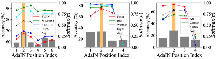
Figure 6: Accuracy by conducting destylization at different positions in a backbone network for 3 different settings: LeNet-5 on Digits, WideResNet (16-4) on CIFAR-10-C, and ResNet-18 on PACS. Positions selected by the NAS algorithm are highlighted in orange. We also visualize the corresponding probabilistic scores ${\rm Softmax}(\pi)$ of Equation 8 in grey.

5 Conclusions

In this paper, we propose a simple yet effective approach for single DG, termed StyDeSty, by introducing the stylization and destylization mechanism. The stylization module aims to generate diversely stylized samples, while the destylization module learns to unify and align the feature distributions. These two designs are co-optimized by a min-max game with a NAS-based method seeking for an optimal position for destylization. StyDeSty is a versatile framework that not only works for classification tasks but is also readily applicable to regression problems. Extensive experiments on multiple benchmarks demonstrate that StyDeSty significantly outperforms the state-of-the-art methods by up to $13.44\%$ in terms of classification accuracy.

Impact Statement

Single domain generalization is a critical area of research in machine learning that aims to enhance the robustness and adaptability of models trained on a single domain when applied to diverse and unseen domains. The impact of this research lies in its potential to significantly improve the deployment of AI systems in real-world scenarios where collecting comprehensive and diverse training data is impractical. By advancing techniques that enable models to generalize from a limited dataset, this work can lead to more reliable and versatile AI applications across various industries, from healthcare and autonomous driving to finance and beyond. Ultimately, single domain generalization fosters the development of more resilient AI systems, contributing to safer and more efficient technological solutions.

In this appendix, we provide more discussion with related works, more analysis, additional details, and more comparison results of the proposed StyDeSty framework for single domain generalization (single DG). First, we summarize related works in a table as a supplement to the related work section of the main paper. Then, we provide some qualitative examples to illustrate the motivation of the proposed method as a supplement to the main paper. We will also give more details on the implementation of the stylization module $G$ and some loss functions. Finally, we conduct more experiments to demonstrate and analyze the performance of our method, including results on more settings and benchmarks, and comparisons on the monocular depth estimation task.

Method	Venue	Key Words	Alignment Loss	Explicit Alignment
JiGen (Carlucci et al., 2019)	CVPR 2019	Jigsaw Puzzles	No	No
RSC (Huang et al., 2020)	ECCV 2020	Self-Challenging	No	No
MMLD (Matsuura & Harada, 2020)	AAAI 2020	Adversarial Augmentation	Yes	No
ADA (Volpi et al., 2018)	NeurIPS 2018	Adversarial Augmentation	No	No
M-ADA (Qiao et al., 2020)	CVPR 2020	Adversarial Augmentation	No	No
ME-ADA (Zhao et al., 2020b)	NeurIPS 2020	Adversarial Augmentation	Yes	No
MixStyle (Zhou et al., 2021)	ICLR 2021	Style Mix-Up	No	No
PDEN (Li et al., 2021)	CVPR 2021	Stylization	Yes	No
L2D (Wang et al., 2021b)	ICCV 2021	Stylization	Yes	No
MetaCNN (Wan et al., 2022)	CVPR 2022	Meta Feature Learning	No	No
CIRL (Lv et al., 2022)	CVPR 2022	Causality	Yes	No
ABA (Cheng et al., 2023)	CVPR 2023	Adversarial Augmentation	Yes	No
MAD (Qu et al., 2023)	CVPR 2023	Debiasing	No	No
Meta-Causal (Chen et al., 2023)	CVPR 2023	Causality	Yes	No
ProRandConv (Choi et al., 2023)	CVPR 2023	Augmentation	No	No
Ours	ICML 2024	Stylization and Destylization	Yes	Yes

Table 7: Summary of related works on single domain generalization methods.

Appendix A Summary of Related Works

We summarize the related works of single domain generalization methods in Tab. 7, focusing on method keywords, alignment loss, and explicit alignment. With the regularization of both alignment loss and explicit alignment in destylization, our method achieves superior single-domain generalization performance.

Appendix B Motivation

Here, as a supplement to Figure 3 of the main paper, we provide further qualitative analysis to the three key questions: why, how, and where to destyle in single DG?

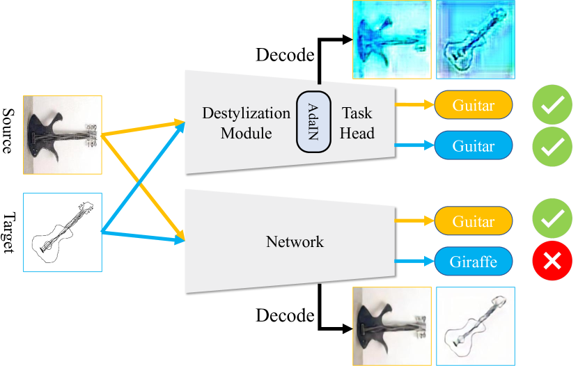
Figure 7: The explicit destylization mechanism unifies styles of the source domain and any unseen target domains, which benefits the performance of the downstream task head.

Why to Destyle? Intuitively, the destylization module in this paper aims to transfer any unseen styles in the test time to the one most familiar to the task head. As shown in Figure 7(top), we decode features after the destylization AdaIN layer to the image space with a pre-trained decoder and find that styles of the source domain (photo) and the unseen target domain (sketch) are aligned, which benefits the following task head. By contrast, in Figure 7(bottom), without explicit destylization, the network is less robust to domain shift and results in inferior performance. There is another example in the plot (a) of Figure 8 to illustrate this effect.

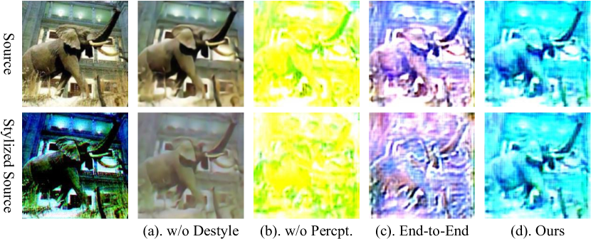
Figure 8: Qualitative results by different fashions of destylization.

How to Destyle? In this paper, there are two metrics to measure the effectiveness of destylization: the element-wise feature distance and the task-perceptual term measured in the space of the task head. On the one hand, if only the former one is adopted, the destylization module would not realize what properties are important for the following task. As shown in plot (b) of Figure 8, although the overall styles are aligned, the major semantic structure is destroyed, which harms the downstream classification. On the other hand, if the task head for measuring the perceptual loss is trained jointly with the destylization module, the task head would also contribute to the destylization, which weakens the ability of alignment for the destylization module. As shown in the plot (c), the alignment is not satisfactory enough compared with that in the plot (d).

Where to Destyle? In the StyDeSty framework, the performance is sensitive to the location of the destylization layer AdaIN in a network. As shown in Figure 9, as the location of destylization goes deeper, the alignment becomes more convenient but more discriminative information is lost. The trade-off between alignment and knowledge for the task motivates us to propose a NAS algorithm for better interaction among stylization, destylization, and the task module.

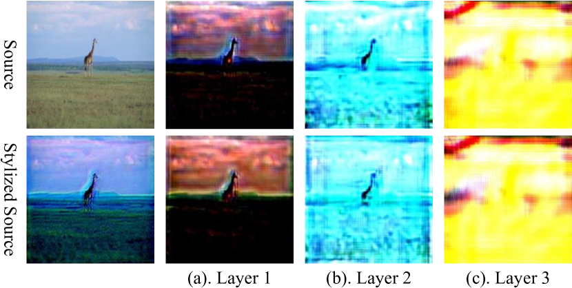
Figure 9: Qualitative results by destylization at different locations.

Appendix C Model Details

Stylization Module. As mentioned in the main paper, the stylization module $G$ consists of $B$ encoder-transformation-decoder blocks. All encoders take the form of a single convolution layer, and all decoders take the form of a symmetric deconvolution layer. Encoders project an image to a $c$-dimension feature space $\mathbb{R}^{h\times w\times c}$, and then the transformation layer learns to conduct affine transformation in this space. The affine parameters for some blocks have shape $h\times w\times c$ to account for local distortions, and parameters for others have shape $1\times 1\times c$ to account for global distortions.

In the experiments on small images with a $32\times 32$ resolution, such as CIFAR-10-C (Hendrycks & Dietterich, 2019; Krizhevsky et al., 2009) and Digits (LeCun et al., 1998; Netzer et al., 2011; Ganin & Lempitsky, 2015; Denker et al., 1988) datasets, the stylization module uses $2$ blocks with local transformation for one and global transformation for another. The number of channels for both blocks is $3$ and the kernel size is $3$. For other classification tasks, the resolution of $224\times 224$ is used, and we use 4 blocks with local transformation and 2 with global transformation. The local transformation blocks have $3$ channels and kernel sizes are $5$, $9$, $13$, and $17$. For the global transformation blocks, one has $3$ channels and a kernel size of $3$, while the other has $64$ channels and a kernel size of $5$. The parameters of convolutional encoders and decoders are random for each iteration.

Metric of Perceptual Distance. The feature alignment loss $\mathcal{L}_{align.}$ is a vital component of the objective for the destylization module $F$. It consists of two terms: $L2$ distance between two feature maps $F(x^{\mathcal{S}})$ and $F(x^{\mathcal{T}})$, and perceptual distance between $H_{-1}(F(x^{\mathcal{S}}))$ and $H_{-1}(F(x^{\mathcal{T}}))$, where $H_{-1}$ extracts features in the last hidden layer of the task head $H$, denoted as $h^{\mathcal{S}}$ and $h^{\mathcal{T}}$ for simplicity.

To measure the distance between $h^{\mathcal{S}}$ and $h^{\mathcal{T}}$, we adopt the following negative log-likelihood (Cheng et al., 2020):

$$-\frac{1}{n}\sum_{i=1}^{n}\log q_{\theta}(h_{i}^{\mathcal{T}}|h_{i}^{\mathcal{S}}),$$

which employs a neural network parameterized by $\theta$ for variational inference. Please refer to (Cheng et al., 2020) for the details.

Semantic Consistency Constraint. To prevent the stylization module from destroying the semantic structures of an image and even generating meaningless results, a semantic consistency constraint that incorporates a semantic perceptron $M$ is included as one supervision signal for this module. Specifically, for the classification task, since the task itself is for semantic understanding, we directly adopt the task network, including the destylization module and the task head without the final linear layer, as the perceptron $M$. For tasks not directly related to semantic understanding like depth estimation, we introduce a pre-trained VGG19 encoder (Simonyan & Zisserman, 2014) as $M$, the semantic loss is measured on 5 layers: ReLU-x_1 for $1\leq x\leq 5$.

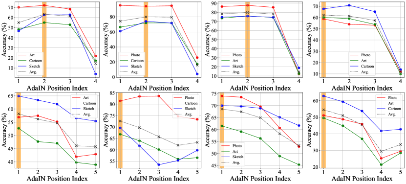
Figure 10: Accuracy results by conducting destylization at different positions in a backbone network for 4 training domains (photo, art painting, cartoon, and sketch for each column respectively) and 2 backbones (ResNet-18 and AlexNet for each row respectively) on PACS dataset. Positions selected by the NAS algorithm are highlighted in orange.

Settings		Source Only	JiGen	RSC	MMLD	ADA	ME-ADA	MixStyle	L2D	Ours
Photo	Art	48.19	56.10	52.88	58.64	53.61	51.76	51.06	58.45	56.93
	Cartoon	43.30	43.52	38.69	49.87	45.44	44.67	41.42	49.74	52.73
	Sketch	51.31	52.46	48.69	50.24	49.02	50.62	48.06	55.82	64.95
	Avg.	47.60	50.69	46.85	52.92	49.36	49.02	46.85	54.67	58.21
Art	Photo	80.24	84.07	85.21	90.36	81.44	81.38	81.42	87.43	81.44
	Cartoon	61.05	65.23	60.54	60.49	61.48	59.68	58.81	69.03	66.81
	Sketch	57.80	62.10	58.74	51.77	59.94	58.84	56.56	66.38	69.61
	Avg.	66.36	70.47	68.16	67.54	67.62	66.64	65.60	74.28	72.62
Cartoon	Photo	64.91	79.58	73.41	85.57	68.86	68.50	66.74	76.95	74.01
	Art	49.07	58.25	53.65	61.72	51.86	53.17	50.53	62.45	61.52
	Sketch	58.74	64.49	63.76	61.82	58.56	56.53	57.44	67.07	69.99
	Avg.	57.88	67.44	63.58	69.70	59.76	59.40	58.24	68.82	68.51
Sketch	Photo	39.88	48.74	53.71	53.05	38.02	38.26	41.01	46.17	51.08
	Art	31.84	37.60	39.94	43.51	32.08	32.37	34.53	35.50	49.56
	Cartoon	52.18	54.39	54.52	61.43	54.95	55.38	55.21	57.98	62.76
	Avg.	41.30	46.91	49.39	53.38	41.68	42.00	43.58	46.55	54.46
Avg.		53.29	58.88	57.00	60.89	54.61	54.27	53.57	61.08	63.45

Table 8: Comparisons of single DG accuracy (%) on PACS dataset. The first column indicates the training domain while the second column indicates the unseen test domain. Results under the AlexNet backbone are reported. Best performances in comparisons are highlighted in bold and the second best ones are marked with underlines.

Settings		Source Only	JiGen	RSC	MMLD	ADA	ME-ADA	MixStyle	L2D	Ours
Photo	Art	64.75	47.85	60.11	57.13	62.30	63.62	58.60	64.84	67.53
	Cartoon	33.15	27.99	35.45	22.44	35.71	35.84	19.49	46.12	50.00
	Sketch	29.12	26.80	40.06	17.43	31.53	30.24	19.30	53.19	61.92
	Avg.	42.34	34.21	45.21	32.33	43.18	43.23	32.46	54.72	59.82
Art	Photo	83.72	85.99	87.78	90.18	94.25	91.86	95.22	92.22	84.97
	Cartoon	57.68	47.53	64.46	54.82	61.52	68.94	52.34	71.54	69.75
	Sketch	42.73	35.81	60.72	46.81	52.51	48.59	35.62	64.21	69.23
	Avg.	61.38	56.44	70.99	63.94	69.43	69.80	61.06	75.99	74.65
Cartoon	Photo	75.25	77.60	72.69	80.60	84.37	82.40	84.74	88.32	84.13
	Art	63.28	56.49	57.56	57.28	62.84	61.96	58.78	72.80	72.51
	Sketch	54.03	45.41	67.40	50.47	59.97	57.62	48.64	64.88	70.37
	Avg.	64.19	59.84	65.89	62.78	69.05	67.33	64.05	75.33	75.67
Sketch	Photo	35.30	40.42	45.09	37.01	40.18	39.94	49.97	55.51	53.95
	Art	37.74	38.13	50.78	38.33	40.43	38.87	38.16	41.26	52.34
	Cartoon	57.64	37.46	64.46	44.03	62.29	59.17	55.52	58.53	64.59
	Avg.	43.56	38.67	53.44	39.79	47.63	45.99	47.88	51.77	55.96
Avg.		52.87	47.27	58.88	49.71	57.32	56.59	51.36	64.45	66.53

Table 9: Comparisons of single DG accuracy (%) on PACS dataset. The first column indicates the training domain while the second column indicates the unseen test domain. Results under the VGG11 backbone are reported. Best performances in comparisons are highlighted in bold and the second best ones are marked with underlines.

Appendix D More Results

Full results on PACS dataset. In this part, we provide full results of single domain generalization using the 4 domains in the PACS dataset (Li et al., 2017) one by one as the training domain. Methods for comparison are the same as those in the main paper, including JiGen (Carlucci et al., 2019), RSC (Huang et al., 2020), MMLD (Matsuura & Harada, 2020), ADA (Volpi et al., 2018), ME-ADA (Zhao et al., 2020a), MixStyle (Zhou et al., 2021), and L2D (Wang et al., 2021b), as well as the baseline method Source Only. The results under ResNet-18 (He et al., 2016) and AlexNet (Krizhevsky et al., 2012) backbones are shown in Tab. 2 and Tab. 8 respectively.

Through the results, we can observe that our StyDeSty outperforms previous state-of-the-art methods in most cases, which is consistent with the conclusion in the main paper. Notably, our method is more robust compared with others when the domain shift is dramatic. For example, when the training or testing domain is Sketch, our method can produce consistent improvement. On average, our method achieves $6.85\%$ and $2.37\%$ promotion over the previous state of the arts.

For ResNet18, NAS chooses the position after the second residual block when the training domain is photo, art painting, and cartoon and the position after the first residual block when the training domain is sketch, to insert the destylization layer. For the AlexNet backbone, the selected position is after the first convolution stage for all four training domains. To demonstrate the effectiveness of the NAS algorithm, we experiment with all the candidate positions for inserting the destylization AdaIN layer. The results of using the two backbone networks on the four training domains are shown as the eight plots in Figure 10 respectively, as a supplement to Figure 6 in the main paper. It proves that the NAS algorithm is competent to find an optimal position in a backbone network to conduct the destylization.

To further explore the capacity of the NAS algorithm, we also experiment with the VGG11 (Simonyan & Zisserman, 2014) backbone on the PACS dataset. The full results are shown in Tab. 9. In this experiment, we choose positions after the 8 ReLU layers as candidate positions for the AdaIN layer. The NAS algorithm chooses ReLU-1_1 layer for art painting and sketch domain and ReLU-2_1 layer for photo and cartoon. We empirically find that when the number of candidates is larger than $10$, the convergence of the NAS algorithm would become difficult, e.g., if we select position after all the $20$ functionality layers in the feature extractor of VGG11 as candidates, the solution would sway among several adjacent layers. More advanced NAS algorithms such as coarse-to-fine strategies are necessary to handle larger backbone networks. Involving multiple destylization layers in a backbone network is also a promising future research direction.

We also conduct experiments on state-of-the-art network backbones like ConvNeXt (Liu et al., 2022c) and SWIN (Liu et al., 2021b). The results of our method and the L2D (Wang et al., 2021b) baseline are shown in Tab. 10. The models are trained on the Photo domain and evaluated on the Art Painting, Cartoon, and Sketch domains. The AdaIN layer is inserted after the second stage for ConvNeXt and after the first stage for SWIN. The results indicate that our method outperforms the baseline without explicit destylization significantly.

Backbone	Method	A	C	S	Avg.
ConvNeXt	L2D	60.32	53.49	67.76	60.52
	Ours	66.20	54.98	74.09	65.09
SWIN	L2D	74.80	49.29	52.77	57.95
	Ours	72.92	52.93	61.26	62.37

Table 10: Comparisons of single DG accuracy (%) on PACS dataset. The models are trained in the Photo domain and evaluated on the Art Painting (A), Cartoon (C), and Sketch (S) domains. Results under ConvNeXt-T and SWIN-T backbones are reported.

Results on DomainNet Dataset. To demonstrate the scalability of the proposed StyDeSty framework for single DG, we conduct experiments on DomainNet dataset (Peng et al., 2019), which consists of images from six distinct domains, including photos (real), clipart, infograph, painting, quickdraw, and sketch. There are 48k to 172k images in each domain and 600k in total that are categorized into 345 classes. We train the ResNet-18 models on the photos and evaluate them on the other 5 domains. The results of our model and the L2D (Wang et al., 2021b) baseline are shown in Tab. 11, where our methods yield consistent improvement.

Comparison on Monocular Depth Estimation. As a supplement to the quantitative results of monocular depth estimation in the main manuscript, we provide qualitative comparisons with those methods without restriction on the label format, including MixStyle (Zhou et al., 2021) and a variant of L2D (Wang et al., 2021b) by removing the class-conditional terms that are incompatible with this task, denoted as v-L2D. Using vKITTI (Gaidon et al., 2016) as the source domain, results on the test KITTI dataset (Geiger et al., 2013) are shown in Figure 11. Through the figure, we can observe that the results of our method show clear object boundaries with the least noise, which demonstrates the superiority of our method over the previous approaches.

Method	C	I	P	Q	S	Avg.
L2D	38.69	12.04	38.40	6.53	30.12	25.16
Ours	42.93	12.79	40.72	6.78	32.67	27.18

Table 11: Comparisons of single DG accuracy (%) on DomainNet. The models are trained on the Photo domain and evaluated on Clipart (C), Infograph (I), Painting (P), Quickdraw (Q), and Sketch (S). Results under the ResNet-18 backbone are reported.

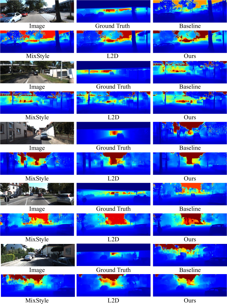
Figure 11: Qualitative comparisons on the monocular depth estimation task. The results of our method demonstrate clearer object boundaries with the least noise.

References

- Albuquerque et al. (2019) Albuquerque, I., Monteiro, J., Darvishi, M., Falk, T. H., and Mitliagkas, I. Generalizing to unseen domains via distribution matching. arXiv preprint arXiv:1911.00804, 2019.
- Balaji et al. (2018) Balaji, Y., Sankaranarayanan, S., and Chellappa, R. Metareg: Towards domain generalization using meta-regularization. Advances in neural information processing systems, 31, 2018.
- Ben-David et al. (2010) Ben-David, S., Blitzer, J., Crammer, K., Kulesza, A., Pereira, F., and Vaughan, J. W. A theory of learning from different domains. Machine learning, 79(1):151–175, 2010.
- Carlucci et al. (2019) Carlucci, F. M., D’Innocente, A., Bucci, S., Caputo, B., and Tommasi, T. Domain generalization by solving jigsaw puzzles. In Proceedings of the IEEE/CVF Conference on Computer Vision and Pattern Recognition, pp. 2229–2238, 2019.
- Chattopadhyay et al. (2020) Chattopadhyay, P., Balaji, Y., and Hoffman, J. Learning to balance specificity and invariance for in and out of domain generalization. In European Conference on Computer Vision, pp. 301–318. Springer, 2020.
- Chen et al. (2022) Chen, C., Li, Z., Ouyang, C., Sinclair, M., Bai, W., and Rueckert, D. Maxstyle: Adversarial style composition for robust medical image segmentation. In International Conference on Medical Image Computing and Computer-Assisted Intervention, pp. 151–161. Springer, 2022.
- Chen et al. (2023) Chen, J., Gao, Z., Wu, X., and Luo, J. Meta-causal learning for single domain generalization. In Proceedings of the IEEE/CVF Conference on Computer Vision and Pattern Recognition, pp. 7683–7692, 2023.
- Cheng et al. (2020) Cheng, P., Hao, W., Dai, S., Liu, J., Gan, Z., and Carin, L. Club: A contrastive log-ratio upper bound of mutual information. In International conference on machine learning, pp. 1779–1788. PMLR, 2020.
- Cheng et al. (2023) Cheng, S., Gokhale, T., and Yang, Y. Adversarial bayesian augmentation for single-source domain generalization. In Proceedings of the IEEE/CVF International Conference on Computer Vision, pp. 11400–11410, 2023.
- Choi et al. (2023) Choi, S., Das, D., Choi, S., Yang, S., Park, H., and Yun, S. Progressive random convolutions for single domain generalization. In Proceedings of the IEEE/CVF Conference on Computer Vision and Pattern Recognition, pp. 10312–10322, 2023.
- Cubuk et al. (2018) Cubuk, E. D., Zoph, B., Mané, D., Vasudevan, V., and Le, Q. V. Autoaugment: Learning augmentation policies from data. CoRR, abs/1805.09501, 2018. URL http://arxiv.org/abs/1805.09501.
- Cugu et al. (2022) Cugu, I., Mancini, M., Chen, Y., and Akata, Z. Attention consistency on visual corruptions for single-source domain generalization. In Proceedings of the IEEE/CVF Conference on Computer Vision and Pattern Recognition, pp. 4165–4174, 2022.
- Denker et al. (1988) Denker, J., Gardner, W., Graf, H., Henderson, D., Howard, R., Hubbard, W., Jackel, L. D., Baird, H., and Guyon, I. Neural network recognizer for hand-written zip code digits. Advances in neural information processing systems, 1, 1988.
- Dou et al. (2019) Dou, Q., Coelho de Castro, D., Kamnitsas, K., and Glocker, B. Domain generalization via model-agnostic learning of semantic features. Advances in Neural Information Processing Systems, 32, 2019.
- Du et al. (2020) Du, Y., Xu, J., Xiong, H., Qiu, Q., Zhen, X., Snoek, C. G., and Shao, L. Learning to learn with variational information bottleneck for domain generalization. In European Conference on Computer Vision, pp. 200–216. Springer, 2020.
- Edwards (2011) Edwards, D. A. On the kantorovich–rubinstein theorem. Expositiones Mathematicae, 29(4):387–398, 2011.
- Fan et al. (2021) Fan, X., Wang, Q., Ke, J., Yang, F., Gong, B., and Zhou, M. Adversarially adaptive normalization for single domain generalization. In Proceedings of the IEEE/CVF Conference on Computer Vision and Pattern Recognition, pp. 8208–8217, 2021.
- Fu et al. (2023) Fu, Y., Xie, Y., Fu, Y., and Jiang, Y.-G. Styleadv: Meta style adversarial training for cross-domain few-shot learning. In Proceedings of the IEEE/CVF Conference on Computer Vision and Pattern Recognition, pp. 24575–24584, 2023.
- Gaidon et al. (2016) Gaidon, A., Wang, Q., Cabon, Y., and Vig, E. Virtual worlds as proxy for multi-object tracking analysis. In Proceedings of the IEEE conference on computer vision and pattern recognition, pp. 4340–4349, 2016.
- Ganin & Lempitsky (2015) Ganin, Y. and Lempitsky, V. Unsupervised domain adaptation by backpropagation. In International conference on machine learning, pp. 1180–1189. PMLR, 2015.
- Gatys et al. (2016) Gatys, L. A., Ecker, A. S., and Bethge, M. Image style transfer using convolutional neural networks. In 2016 IEEE Conference on Computer Vision and Pattern Recognition, CVPR 2016, Las Vegas, NV, USA, June 27-30, 2016, pp. 2414–2423. IEEE Computer Society, 2016. doi: 10.1109/CVPR.2016.265. URL https://doi.org/10.1109/CVPR.2016.265.
- Geiger et al. (2013) Geiger, A., Lenz, P., Stiller, C., and Urtasun, R. Vision meets robotics: The kitti dataset. The International Journal of Robotics Research, 32(11):1231–1237, 2013.
- He et al. (2016) He, K., Zhang, X., Ren, S., and Sun, J. Deep residual learning for image recognition. In Proceedings of the IEEE conference on computer vision and pattern recognition, pp. 770–778, 2016.
- Hendrycks & Dietterich (2019) Hendrycks, D. and Dietterich, T. Benchmarking neural network robustness to common corruptions and perturbations. arXiv preprint arXiv:1903.12261, 2019.
- Huang & Belongie (2017) Huang, X. and Belongie, S. Arbitrary style transfer in real-time with adaptive instance normalization. In Proceedings of the IEEE international conference on computer vision, pp. 1501–1510, 2017.
- Huang et al. (2020) Huang, Z., Wang, H., Xing, E. P., and Huang, D. Self-challenging improves cross-domain generalization. In European Conference on Computer Vision, pp. 124–140. Springer, 2020.
- Jang et al. (2016) Jang, E., Gu, S., and Poole, B. Categorical reparameterization with gumbel-softmax. arXiv preprint arXiv:1611.01144, 2016.
- Jin et al. (2020) Jin, X., Lan, C., Zeng, W., and Chen, Z. Feature alignment and restoration for domain generalization and adaptation. arXiv preprint arXiv:2006.12009, 2020.
- Jin et al. (2021) Jin, X., Lan, C., Zeng, W., and Chen, Z. Style normalization and restitution for domain generalization and adaptation. IEEE Transactions on Multimedia, 2021.
- Kang et al. (2022) Kang, J., Lee, S., Kim, N., and Kwak, S. Style neophile: Constantly seeking novel styles for domain generalization. In Proceedings of the IEEE/CVF Conference on Computer Vision and Pattern Recognition, pp. 7130–7140, 2022.
- Kingma & Ba (2014) Kingma, D. P. and Ba, J. Adam: A method for stochastic optimization. arXiv preprint arXiv:1412.6980, 2014.
- Krizhevsky et al. (2009) Krizhevsky, A., Hinton, G., et al. Learning multiple layers of features from tiny images. 2009.
- Krizhevsky et al. (2012) Krizhevsky, A., Sutskever, I., and Hinton, G. E. Imagenet classification with deep convolutional neural networks. Advances in neural information processing systems, 25, 2012.
- LeCun et al. (1998) LeCun, Y., Bottou, L., Bengio, Y., and Haffner, P. Gradient-based learning applied to document recognition. Proceedings of the IEEE, 86(11):2278–2324, 1998.
- Li et al. (2017) Li, D., Yang, Y., Song, Y.-Z., and Hospedales, T. M. Deeper, broader and artier domain generalization. In Proceedings of the IEEE international conference on computer vision, pp. 5542–5550, 2017.
- Li et al. (2019) Li, D., Zhang, J., Yang, Y., Liu, C., Song, Y.-Z., and Hospedales, T. M. Episodic training for domain generalization. In Proceedings of the IEEE/CVF International Conference on Computer Vision, pp. 1446–1455, 2019.
- Li et al. (2018a) Li, H., Pan, S. J., Wang, S., and Kot, A. C. Domain generalization with adversarial feature learning. In Proceedings of the IEEE conference on computer vision and pattern recognition, pp. 5400–5409, 2018a.
- Li et al. (2021) Li, L., Gao, K., Cao, J., Huang, Z., Weng, Y., Mi, X., Yu, Z., Li, X., and Xia, B. Progressive domain expansion network for single domain generalization. In Proceedings of the IEEE/CVF Conference on Computer Vision and Pattern Recognition, pp. 224–233, 2021.
- Li et al. (2018b) Li, Y., Tian, X., Gong, M., Liu, Y., Liu, T., Zhang, K., and Tao, D. Deep domain generalization via conditional invariant adversarial networks. In Proceedings of the European Conference on Computer Vision (ECCV), pp. 624–639, 2018b.
- Liu et al. (2020) Liu, S., Wu, H., Luo, S., and Sun, Z. Stable video style transfer based on partial convolution with depth-aware supervision. In Chen, C. W., Cucchiara, R., Hua, X., Qi, G., Ricci, E., Zhang, Z., and Zimmermann, R. (eds.), MM ’20: The 28th ACM International Conference on Multimedia, Virtual Event / Seattle, WA, USA, October 12-16, 2020, pp. 2445–2453. ACM, 2020. doi: 10.1145/3394171.3413526. URL https://doi.org/10.1145/3394171.3413526.
- Liu et al. (2021a) Liu, S., Lin, T., He, D., Li, F., Wang, M., Li, X., Sun, Z., Li, Q., and Ding, E. Adaattn: Revisit attention mechanism in arbitrary neural style transfer. In 2021 IEEE/CVF International Conference on Computer Vision, ICCV 2021, Montreal, QC, Canada, October 10-17, 2021, pp. 6629–6638. IEEE, 2021a. doi: 10.1109/ICCV48922.2021.00658. URL https://doi.org/10.1109/ICCV48922.2021.00658.
- Liu et al. (2022a) Liu, S., Wang, K., Yang, X., Ye, J., and Wang, X. Dataset distillation via factorization. In Proceedings of the Advances in Neural Information Processing Systems (NeurIPS), 2022a.
- Liu et al. (2022b) Liu, S., Ye, J., Ren, S., and Wang, X. Dynast: Dynamic sparse transformer for exemplar-guided image generation. In Avidan, S., Brostow, G. J., Cissé, M., Farinella, G. M., and Hassner, T. (eds.), Computer Vision - ECCV 2022 - 17th European Conference, Tel Aviv, Israel, October 23-27, 2022, Proceedings, Part XVI, volume 13676 of Lecture Notes in Computer Science, pp. 72–90. Springer, 2022b. doi: 10.1007/978-3-031-19787-1“˙5. URL https://doi.org/10.1007/978-3-031-19787-1_5.
- Liu et al. (2023) Liu, S., Ye, J., and Wang, X. Any-to-any style transfer: Making picasso and da vinci collaborate. CoRR, abs/2304.09728, 2023. doi: 10.48550/ARXIV.2304.09728. URL https://doi.org/10.48550/arXiv.2304.09728.
- Liu et al. (2021b) Liu, Z., Lin, Y., Cao, Y., Hu, H., Wei, Y., Zhang, Z., Lin, S., and Guo, B. Swin transformer: Hierarchical vision transformer using shifted windows. In Proceedings of the IEEE/CVF International Conference on Computer Vision (ICCV), 2021b.
- Liu et al. (2022c) Liu, Z., Mao, H., Wu, C.-Y., Feichtenhofer, C., Darrell, T., and Xie, S. A convnet for the 2020s. Proceedings of the IEEE/CVF Conference on Computer Vision and Pattern Recognition (CVPR), 2022c.
- Long et al. (2015) Long, M., Cao, Y., Wang, J., and Jordan, M. Learning transferable features with deep adaptation networks. In ICML, pp. 97–105, 2015.
- Lv et al. (2022) Lv, F., Liang, J., Li, S., Zang, B., Liu, C. H., Wang, Z., and Liu, D. Causality inspired representation learning for domain generalization. In Proceedings of the IEEE/CVF conference on computer vision and pattern recognition, pp. 8046–8056, 2022.
- Mahajan et al. (2021) Mahajan, D., Tople, S., and Sharma, A. Domain generalization using causal matching. In International Conference on Machine Learning, pp. 7313–7324. PMLR, 2021.
- Matsuura & Harada (2020) Matsuura, T. and Harada, T. Domain generalization using a mixture of multiple latent domains. In Proceedings of the AAAI Conference on Artificial Intelligence, volume 34, pp. 11749–11756, 2020.
- Motiian et al. (2017) Motiian, S., Piccirilli, M., Adjeroh, D. A., and Doretto, G. Unified deep supervised domain adaptation and generalization. In Proceedings of the IEEE international conference on computer vision, pp. 5715–5725, 2017.
- Muandet et al. (2013) Muandet, K., Balduzzi, D., and Schölkopf, B. Domain generalization via invariant feature representation. In International Conference on Machine Learning, pp. 10–18. PMLR, 2013.
- Nesterov (1983) Nesterov, Y. A method for unconstrained convex minimization problem with the rate of convergence o (1/k^ 2). In Doklady an ussr, volume 269, pp. 543–547, 1983.
- Netzer et al. (2011) Netzer, Y., Wang, T., Coates, A., Bissacco, A., Wu, B., and Ng, A. Y. Reading digits in natural images with unsupervised feature learning. 2011.
- Peng et al. (2019) Peng, X., Bai, Q., Xia, X., Huang, Z., Saenko, K., and Wang, B. Moment matching for multi-source domain adaptation. In ICCV, pp. 1406–1415, 2019.
- Qiao et al. (2020) Qiao, F., Zhao, L., and Peng, X. Learning to learn single domain generalization. In Proceedings of the IEEE/CVF Conference on Computer Vision and Pattern Recognition, pp. 12556–12565, 2020.
- Qu et al. (2023) Qu, S., Pan, Y., Chen, G., Yao, T., Jiang, C., and Mei, T. Modality-agnostic debiasing for single domain generalization. In Proceedings of the IEEE/CVF Conference on Computer Vision and Pattern Recognition, pp. 24142–24151, 2023.
- Radford et al. (2016) Radford, A., Metz, L., and Chintala, S. Unsupervised representation learning with deep convolutional generative adversarial networks. In Bengio, Y. and LeCun, Y. (eds.), 4th International Conference on Learning Representations, ICLR 2016, San Juan, Puerto Rico, May 2-4, 2016, Conference Track Proceedings, 2016. URL http://arxiv.org/abs/1511.06434.
- Ronneberger et al. (2015) Ronneberger, O., Fischer, P., and Brox, T. U-net: Convolutional networks for biomedical image segmentation. In International Conference on Medical image computing and computer-assisted intervention, pp. 234–241. Springer, 2015.
- Russakovsky et al. (2015) Russakovsky, O., Deng, J., Su, H., Krause, J., Satheesh, S., Ma, S., Huang, Z., Karpathy, A., Khosla, A., Bernstein, M., et al. Imagenet large scale visual recognition challenge. International journal of computer vision, 115(3):211–252, 2015.
- Seo et al. (2020) Seo, S., Suh, Y., Kim, D., Kim, G., Han, J., and Han, B. Learning to optimize domain specific normalization for domain generalization. In European Conference on Computer Vision, pp. 68–83. Springer, 2020.
- Shao et al. (2019) Shao, R., Lan, X., Li, J., and Yuen, P. C. Multi-adversarial discriminative deep domain generalization for face presentation attack detection. In Proceedings of the IEEE/CVF Conference on Computer Vision and Pattern Recognition, pp. 10023–10031, 2019.
- Simonyan & Zisserman (2014) Simonyan, K. and Zisserman, A. Very deep convolutional networks for large-scale image recognition. arXiv preprint arXiv:1409.1556, 2014.
- Sinha et al. (2017) Sinha, A., Namkoong, H., Volpi, R., and Duchi, J. Certifying some distributional robustness with principled adversarial training. arXiv preprint arXiv:1710.10571, 2017.
- Sun & Saenko (2016) Sun, B. and Saenko, K. Deep coral: Correlation alignment for deep domain adaptation. In ECCV, pp. 443–450, 2016.
- Tang et al. (2023) Tang, H., Liu, S., Lin, T., Huang, S., Li, F., He, D., and Wang, X. Master: Meta style transformer for controllable zero-shot and few-shot artistic style transfer. In IEEE/CVF Conference on Computer Vision and Pattern Recognition, CVPR 2023, Vancouver, BC, Canada, June 17-24, 2023, pp. 18329–18338. IEEE, 2023. doi: 10.1109/CVPR52729.2023.01758. URL https://doi.org/10.1109/CVPR52729.2023.01758.
- Van der Maaten & Hinton (2008) Van der Maaten, L. and Hinton, G. Visualizing data using t-sne. Journal of machine learning research, 9(11), 2008.
- Volpi & Murino (2019) Volpi, R. and Murino, V. Addressing model vulnerability to distributional shifts over image transformation sets. In Proceedings of the IEEE/CVF International Conference on Computer Vision, pp. 7980–7989, 2019.
- Volpi et al. (2018) Volpi, R., Namkoong, H., Sener, O., Duchi, J. C., Murino, V., and Savarese, S. Generalizing to unseen domains via adversarial data augmentation. Advances in neural information processing systems, 31, 2018.
- Wan et al. (2022) Wan, C., Shen, X., Zhang, Y., Yin, Z., Tian, X., Gao, F., Huang, J., and Hua, X.-S. Meta convolutional neural networks for single domain generalization. In Proceedings of the IEEE/CVF Conference on Computer Vision and Pattern Recognition, pp. 4682–4691, 2022.
- Wang et al. (2019a) Wang, H., Ge, S., Lipton, Z., and Xing, E. P. Learning robust global representations by penalizing local predictive power. Advances in Neural Information Processing Systems, 32, 2019a.
- Wang et al. (2019b) Wang, H., He, Z., Lipton, Z. C., and Xing, E. P. Learning robust representations by projecting superficial statistics out. arXiv preprint arXiv:1903.06256, 2019b.
- Wang et al. (2021a) Wang, J., Lan, C., Liu, C., Ouyang, Y., Zeng, W., and Qin, T. Generalizing to unseen domains: A survey on domain generalization. arXiv preprint arXiv:2103.03097, 2021a.
- Wang et al. (2021b) Wang, Z., Luo, Y., Qiu, R., Huang, Z., and Baktashmotlagh, M. Learning to diversify for single domain generalization. In Proceedings of the IEEE/CVF International Conference on Computer Vision, pp. 834–843, 2021b.
- Yan et al. (2017) Yan, H., Ding, Y., Li, P., Wang, Q., Xu, Y., and Zuo, W. Mind the class weight bias: Weighted maximum mean discrepancy for unsupervised domain adaptation. In CVPR, pp. 2272–2281, 2017.
- Yang et al. (2023) Yang, L., Gu, X., and Sun, J. Generalized semantic segmentation by self-supervised source domain projection and multi-level contrastive learning. In Williams, B., Chen, Y., and Neville, J. (eds.), Thirty-Seventh AAAI Conference on Artificial Intelligence, AAAI 2023, Thirty-Fifth Conference on Innovative Applications of Artificial Intelligence, IAAI 2023, Thirteenth Symposium on Educational Advances in Artificial Intelligence, EAAI 2023, Washington, DC, USA, February 7-14, 2023, pp. 10789–10797. AAAI Press, 2023. doi: 10.1609/AAAI.V37I9.26280. URL https://doi.org/10.1609/aaai.v37i9.26280.
- Yang et al. (2022a) Yang, X., Ye, J., and Wang, X. Factorizing knowledge in neural networks. In European Conference on Computer Vision, 2022a.
- Yang et al. (2022b) Yang, X., Zhou, D., Liu, S., Ye, J., and Wang, X. Deep model reassembly. In Advances in neural information processing systems, 2022b.
- Ye & Wang (2024) Ye, J. and Wang, X. Ungeneralizable examples. In Proceedings of the IEEE/CVF Conference on Computer Vision and Pattern Recognition, 2024.
- Ye et al. (2023) Ye, J., Liu, S., and Wang, X. Partial network cloning. In Proceedings of the IEEE/CVF Conference on Computer Vision and Pattern Recognition, 2023.
- Yu et al. (2023) Yu, R., Liu, S., Yang, X., and Wang, X. Distribution shift inversion for out-of-distribution prediction. In Proceedings of the IEEE/CVF Conference on Computer Vision and Pattern Recognition, 2023.
- Zagoruyko & Komodakis (2016) Zagoruyko, S. and Komodakis, N. Wide residual networks. arXiv preprint arXiv:1605.07146, 2016.
- Zhao et al. (2020a) Zhao, L., Liu, T., Peng, X., and Metaxas, D. Maximum-entropy adversarial data augmentation for improved generalization and robustness. Advances in Neural Information Processing Systems, 33:14435–14447, 2020a.
- Zhao et al. (2019) Zhao, S., Fu, H., Gong, M., and Tao, D. Geometry-aware symmetric domain adaptation for monocular depth estimation. In Proceedings of the IEEE Conference on Computer Vision and Pattern Recognition, pp. 9788–9798, 2019.
- Zhao et al. (2020b) Zhao, S., Gong, M., Liu, T., Fu, H., and Tao, D. Domain generalization via entropy regularization. Advances in Neural Information Processing Systems, 33:16096–16107, 2020b.
- Zhao et al. (2022) Zhao, Y., Zhong, Z., Zhao, N., Sebe, N., and Lee, G. H. Style-hallucinated dual consistency learning for domain generalized semantic segmentation. In European Conference on Computer Vision, pp. 535–552. Springer, 2022.
- Zhong et al. (2022) Zhong, Z., Zhao, Y., Lee, G. H., and Sebe, N. Adversarial style augmentation for domain generalized urban-scene segmentation. Advances in Neural Information Processing Systems, 35:338–350, 2022.
- Zhou et al. (2020) Zhou, K., Yang, Y., Hospedales, T., and Xiang, T. Learning to generate novel domains for domain generalization. In European conference on computer vision, pp. 561–578. Springer, 2020.
- Zhou et al. (2021) Zhou, K., Yang, Y., Qiao, Y., and Xiang, T. Domain generalization with mixstyle. arXiv preprint arXiv:2104.02008, 2021.
- Zhuo et al. (2017) Zhuo, J., Wang, S., Zhang, W., and Huang, Q. Deep unsupervised convolutional domain adaptation. In ACM MM, pp. 261–269. ACM, 2017.