Magnetization in a non-equilibrium quantum spin system

Abstract

The dynamics described by the non-Hermitian Hamiltonian typically capture the short-term behavior of open quantum systems before quantum jumps occur. In contrast, the long-term dynamics, characterized by the Lindblad master equation (LME), drive the system towards a non-equilibrium steady state (NESS), which is an eigenstate with zero energy of the Liouvillian superoperator, denoted as $\mathcal{L}$. Conventionally, these two types of evolutions exhibit distinct dynamical behaviors. However, in this study, we challenge this common belief and demonstrate that the effective non-Hermitian Hamiltonian can accurately represent the long-term dynamics of a critical two-level open quantum system. The criticality of the system arises from the exceptional point (EP) of the effective non-Hermitian Hamiltonian. Additionally, the NESS is identical to the coalescent state of the effective non-Hermitian Hamiltonian. We apply this finding to a series of critical open quantum systems and show that a local dissipation channel can induce collective alignment of all spins in the same direction. This direction can be well controlled by modulating the quantum jump operator. The corresponding NESS is a product state and maintains long-time coherence, facilitating quantum control in open many-body systems. This discovery paves the way for a better understanding of the long-term dynamics of critical open quantum systems.

I Introduction

Open quantum many-body systems have emerged as a captivating research field at the intersection of theoretical and experimental physics Breuer and Petruccione (2002); Weiss (2012); Rivas and Huelga (2012). Comprising numerous interacting quantum particles, these systems exhibit intricate and captivating dynamics that elude traditional closed quantum systems. The interaction of these systems with an external environment leads to dissipation and decoherence, presenting new challenges and opportunities for exploring quantum phenomena Pellizzari et al. (1995); Balasubramanian et al. (2009); Lanyon et al. (2011); Paik et al. (2011). Recent advancements have been made in the realization and manipulation of open quantum many-body systems in atomic, molecular, and optical (AMO) systems Kasprzak et al. (2006); Bloch et al. (2008); Bloch (2008); Diehl et al. (2008); Syassen et al. (2008); Baumann et al. (2010); Barreiro et al. (2011); Schauß et al. (2012); Ritsch et al. (2013); Carusotto and Ciuti (2013); Daley (2014), which offer precise control over individual quantum particles and enable the engineering of complex interactions and dissipation mechanisms. In addition, state-of-the-art measurement techniques, such as quantum state tomography and quantum non-demolition measurements, provide unprecedented opportunities to investigate the dynamics of these systems with high precision Nelson et al. (2007); Gericke et al. (2008); Hofferberth et al. (2008); Bakr et al. (2009); Sherson et al. (2010); Miranda et al. (2015); Cheuk et al. (2015); Parsons et al. (2015); Haller et al. (2015); Omran et al. (2015); Edge et al. (2015); Yamamoto et al. (2016); Alberti et al. (2016).

The dynamics of an open quantum system are typically described by a quantum master equation, specifically the Lindblad master equation (LME). This is attributed to the weak coupling and separation of timescales between the system and its environment. The Liouvillian superoperator $\mathcal{L}$ governs the time evolution of the density matrix, fully characterizing the relaxation dynamics of an open quantum system through its complex spectrum and eigenmodes Rivas and Huelga (2012). A notable feature of open quantum systems is the presence of long-lived states that emerge far from equilibrium, known as non-equilibrium steady states (NESS). These NESS can exhibit novel properties, such as the presence of quantum correlations and the breakdown of conventional statistical mechanics Eisert et al. (2015). Investigating the conditions and properties of NESS is currently an active area of research.

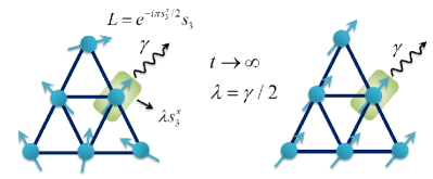
Figure 1: Schematic illustration of the magnetization in a non-equilibrium quantum spin system. The system comprises six spins, with the third spin subjected to a local external field represented as $\lambda s_{3}^{x}$, and a dissipation channel characterized by the quantum jump operator $L=e^{-i\pi s^{x}/2}s_{3}^{-}$. The green-shaded region in the illustration depicts the local external field. The long-lived NESS of the system converges to a coherent product state, with all spins aligning in the same direction, when a critical field is activated. This behavior results from the identical dynamic effects induced by two types of probability of the the SSE in each quantum trajectory. Importantly, this finding remains robust irrespective of the system’s structure and the initial spin configuration.

The non-Hermitian Hamiltonian is an extension of standard quantum mechanics that allows for the description of dissipative systems in a minimalistic manner. In recent years, there has been a growing interest in using non-Hermitian descriptions to study condensed matter systems Lee (2016); Kunst et al. (2018); Yao et al. (2018); Gong et al. (2018); El-Ganainy et al. (2018); Nakagawa et al. (2018); Shen and Fu (2018); Wu et al. (2019); Yamamoto et al. (2019); Song et al. (2019); Yang and Hu (2019); Hamazaki et al. (2019); Li et al. (2019); Kawabata et al. (2019a, b); Lee et al. (2019); Yokomizo and Murakami (2019); Jin et al. (2020) . These descriptions have not only expanded the realm of condensed-matter physics, providing insightful perspectives, but also offered a fruitful framework for understanding inelastic collisions Xu et al. (2017), disorder effects Shen and Fu (2018); Hamazaki et al. (2019), and system-environment couplings Nakagawa et al. (2018); Yang and Hu (2019); Song et al. (2019). The interplay between non-Hermiticity and interactions can lead to exotic quantum many-body effects, such as non-Hermitian extensions of the Kondo effect Nakagawa et al. (2018); Lourenço et al. (2018), many-body localization Hamazaki et al. (2019), and fermionic superfluidity Yamamoto et al. (2019); Okuma and Sato (2019). One intriguing feature of non-Hermitian systems is the presence of exceptional points (EPs), which are degeneracies of non-Hermitian operators where the eigenvalues and corresponding eigenstates merge into a single state Berry (2004); Heiss (2012); Lee (2016); Miri and Alù (2019); Zhang and Gong (2020). These EPs give rise to fascinating dynamical phenomena, including asymmetric mode switching Doppler et al. (2016), topological energy transfer Xu et al. (2016), robust wireless power transfer Assawaworrarit et al. (2017), and enhanced sensitivity Wiersig (2014, 2016); Hodaei et al. (2017); Chen et al. (2017), depending on the nature of their EP degeneracies. High-order EPs, where more than two eigenstates coalesce, have attracted significant attention due to their topological and distinct dynamical properties Zhang et al. (2012, 2020a, 2020b); Zhang and Song (2020, 2021); Yang and Song (2021); Xu et al. (2023); Xu and Jin (2023).

In the context of open quantum systems, the evolved density matrix driven by the LME can be obtained by averaging an ensemble of quantum trajectories. Each trajectory is determined by the stochastic Schröinger equation (SSE). The SSE involves two types of probability evolution: a non-unitary evolution determined by the effective non-Hermitian Hamiltonian and a state collapse induced by the quantum jump operator. Generally, the non-Hermitian Hamiltonian captures the short-term dynamics of the open quantum system before a quantum jump occurs or describes a post-selected trajectory that necessitates substantial experimental resources. The dynamical consequences of the effective non-Hermitian system are irrelevant to the NESS of the open quantum system. The objective of this paper is to establish the connection between the dynamics determined by the non-Hermitian Hamiltonian and the LME. First, we review the connection between the stochastic SSE and the LME. We demonstrate how to modulate the quantum jump operator to make the evolved state converge to the coalescent state determined by the critical non-Hermitian Hamiltonian in each quantum trajectory. Essentially, the evolution direction dictated by the critical non-Hermitian Hamiltonian coincides with that determined by the quantum jump operator. This is a unique characteristic of the critical non-Hermitian Hamiltonian that lacks in non-Hermitian Hamiltonians without exceptional points (EPs) or imaginary energy levels. Furthermore, we generalize this mechanism to the critical quantum spin system with high-order EPs. We demonstrate that a single local dissipation can cause the collective rotation of spins in a specific direction, which is shown in Fig. 1. The achieved NESS is equivalent to the coalescent state of such a critical non-Hermitian Hamiltonian. Remarkably, this non-equilibrium behavior remains unaffected by the system’s geometry, initial spin configuration, and weak disorder, thus highlighting its robustness. These analytical findings possess independent interest and hold the potential to inspire future analytical studies on critical open quantum systems.

The remainder of the paper is organized as follows: Sec.  II provides a review of the LME and the SSE, demonstrating the underlying mechanism using a two-level open quantum system. Sec. III applies the obtained mechanism to an open quantum spin system. We showcase the coincidence between EP dynamics and the magnetization of the open quantum spin system. Furthermore, we analyze the proposed scheme across various system parameters. We conclude the paper in Sec. IV. Supplementary details of our calculation are provided in the Appendix.

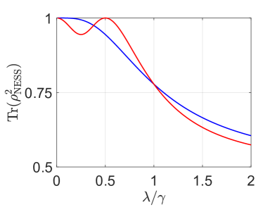
Figure 2: Plot of the purity Tr$\left(\rho_{\mathrm{NESS}}^{2}\right)$ as the function of $\lambda/\gamma$. The blue and red lines correspond to the quantum jump operators $L=s^{-}$, and $\widetilde{L}=e^{-i\frac{\pi}{2}s^{x}}s^{-}$, respectively. The blue line monotonically decreases to $0.5$, indicating a completely mixed state. The red line initially decreases and then returns to $1$. There is a range around $0.5$ where the evolved state can be approximated as a pure state. When $\lambda/\gamma=0.5$, the NESS is $\rho_{\mathrm{NESS}}$ $|y,+\rangle\langle y,+|$, which is also the coalescent of $\mathcal{H}$.

II Heuristic derivation

The dynamics of open quantum systems coupled to a Markovian environment are commonly described by the LME. The equation describing the time evolution of the density matrix $\rho$ is given by

$$\frac{\text{{d}}\rho}{\text{{d}}t}=-i(\mathcal{H}\rho-\rho\mathcal{H}^{\dagger})+\sum_{\mu}\Gamma_{\mu}L_{\mu}\rho L_{\mu}^{\dagger}\equiv\mathcal{L}\rho.$$ (1)

In this equation, $\rho$ represents the density matrix. The non-Hermitian Hamiltonian $\mathcal{H}$ is given by $\mathcal{H}$ $\mathcal{=}$ $H-\frac{i}{2}\sum_{\mu}\Gamma_{\mu}L_{\mu}^{\dagger}L_{\mu}$, where $H$ is a Hermitian operator representing the system Hamiltonian. The non-Hermitian nature of $\mathcal{H}$ accounts for the non-unitary dynamics observed in open quantum systems. The jump operators $L_{\mu}$ describe the dissipative quantum channels with a strength of $\Gamma_{\mu}$. $\mathcal{L}$ is the Liouvillian superoperator. Alternatively, one can track the trajectory of a pure state using a SSE, such as

$$\text{{d}}|\Psi\rangle = -i\mathcal{H}|\Psi\rangle\text{{d}}t+\frac{1}{2}\sum_{\mu}\Gamma_{\mu}[\langle\Psi|L_{\mu}^{\dagger}L_{\mu}|\Psi\rangle]|\Psi\rangle\text{{d}}t$$ (2)

$$+\sum_{\mu}(\frac{L_{\mu}|\Psi\rangle}{\sqrt{\langle\Psi|L_{\mu}^{\dagger}L_{\mu}|\Psi\rangle}}-|\Psi\rangle)\text{{d}}N_{\mu},$$

where the Poisson increment d$N_{\mu}$ satisfies d$N_{\mu}$d$N_{\nu}=\delta_{\mu\nu}$, taking the value $0$ or $1$. The jump operators in the LME correspond to the stochastic jumps in the SSE. If d$N_{\mu}=0$, the evolution is solely described by the non-Hermitian Hamiltonian $\mathcal{H}$, which is referred to as the no-click limit Daley (2014). However, this limit is rarely achieved in experiments since its realization requires exponentially many experiments to be carried out before a desired trajectory is obtained. The connection between the SSE and the LME lies in the relationship between the individual wave function trajectories and the ensemble-averaged density matrix. By averaging over the different realizations of the stochastic trajectories generated by the SSE, one can recover the ensemble-averaged dynamics described by the LME. In this way, the SSE provides a more detailed and microscopic description of the dynamics, while the LME provides a coarse-grained description that captures the averaged behavior of the system Daley (2014).

To fully grasp the essence of this paper, we begin by considering a simple quantum system comprising two levels with orthonormal states. This model has diverse applications and can describe phenomena such as the spin degree of freedom of an electron, a simplified representation of an atom with only two atomic levels, the lowest eigenstates of a superconducting circuit, or the discrete charge states of a quantum dot. In this model, the system Hamiltonian is given by $H=\lambda s^{x}$, where $\lambda$ represents the energy difference between the two states and $\sigma^{x}=2s^{x}$ is the Pauli matrix corresponding to the $x$-direction. The quantum jump operator is denoted as $L_{\mu}=s^{-}$ with a strength $\Gamma_{\mu}=\gamma$, where $s^{-}$ represents the lowering operator responsible for the spin flip from the spin-up state to the spin-down state. The initial state $|\Psi\left(0\right)\rangle$ is assumed to be an arbitrary pure state applicable to various many-body examples. In this context, the initial state is represented by the density matrix $\rho\left(t=0\right)=|\Psi\left(0\right)\rangle\langle\Psi\left(0\right)|$. Referring to the Eq. (2), the evolution of $|\Psi\left(t+\delta t\right)\rangle$ is determined by either $\frac{\left(1-i\mathcal{H}\delta t\right)}{\sqrt{1-\delta p}}|\Psi\left(t\right)\rangle$ with a probability of $1-\delta p$ or $\frac{L}{\sqrt{\delta p/\delta t}}|\Psi\left(t\right)\rangle$ with a probability of $\delta p$. Here $\delta p$ is red defined as

$$\delta p=\langle\Psi\left(t\right)|s^{+}s^{-}|\Psi\left(t\right)\rangle\delta t.$$ (3)

Notice that when $\lambda>\gamma/2$, the state $|\Psi\left(t\right)\rangle$ oscillates between the two eigenstates of the non-Hermitian Hamiltonian $\mathcal{H}$ , which possesses a full real spectrum except for a common imaginary part eliminated by the amplitude $1/\sqrt{1-\delta p}$. On the other hand, if $\lambda<\gamma/2$, $|\Psi\left(t\right)\rangle$ relaxes to the eigenstate with the maximum imaginary part, as $\mathcal{H}$ has two complex eigenvalues. It is worth noting that when $\lambda=\gamma/2$, an exceptional point (EP) exists in the spectrum of $\mathcal{H}$, where there is only one coalescent eigenstate $|\psi_{\mathrm{c}}\rangle=\frac{1}{\sqrt{2}}\left(1,i\right)^{T}$. For an arbitrary initial state $|\Psi\left(0\right)\rangle$, it evolves towards the coalescent state $|\psi_{\mathrm{c}}\rangle$ due to the nilpotent matrix property of $\mathcal{H}$, i.e., $\mathcal{H}^{2}=0$ (see Appendix V.1 for more details). Alternatively, if the final state is a steady pure state, it can be projected onto the Bloch sphere, revealing a definite spin direction. However, the presence of the quantum jump operator $s^{-}$ disrupts the evolution driven by $\mathcal{H}$ and consequently affects the direction. The steady state must strike a balance between these two probabilistic evolutions. To gain further insight into the NESS $\rho_{\mathrm{NESS}}$ defined by d$\left(\rho_{\mathrm{NESS}}\right)/$d$t=0$, we employ a spin bi-base mapping, also known as the Choi-Jamiołkowski isomorphism, to map a density matrix to a vector in the computational bases (see Appendix V.2 for more details). The NESS corresponds to the eigenstate of $\mathcal{L}$ with zero eigenvalue, which can be expressed as

$$\rho_{\mathrm{NESS}}=\left(\begin{array}[]{cc}\frac{\lambda^{2}}{2\lambda^{2}+\gamma^{2}}&-i\frac{\lambda\gamma}{2\lambda^{2}+\gamma^{2}}\\ i\frac{\lambda\gamma}{2\lambda^{2}+\gamma^{2}}&\frac{\lambda^{2}+\gamma^{2}}{2\lambda^{2}+\gamma^{2}}\end{array}\right).$$ (4)

The coherence of a system can be measured by its purity, which is quantified by the function Tr$(\rho_{\mathrm{NESS}}^{2})$. In Fig. 2, we depict the behavior of Tr$(\rho_{\mathrm{NESS}}^{2})$ as a function of $\lambda$, while keeping $\gamma$ fixed at 1. Let us first consider two limiting cases: When $\lambda=0$, the non-Hermitian Hamiltonian $\mathcal{H}$ drives the initial state to $|\psi_{\mathrm{f}}\rangle=(0,1)$. Simultaneously, the quantum jump operator projects the spin to the down state. Consequently, $|\psi_{\mathrm{f}}\rangle$ becomes the non-equilibrium steady state (NESS). On the other hand, when $\lambda\gg\gamma$, the density matrix $\rho_{\mathrm{NESS}}$ simplifies to

$$\rho_{\mathrm{NESS}}=\left(\begin{array}[]{cc}1/2&0\\ 0&1/2\end{array}\right),$$ (5)

which corresponds to a completely mixed state. This can be understood as follows: Under the influence of the non-Hermitian Hamiltonian $\mathcal{H}$, the evolved state does not have a definite direction. Instead, it oscillates between the two eigenvectors along the $x$-direction, i.e., $|\psi_{\mathrm{1}}\rangle=\left(1,\text{ }1\right)^{T}/\sqrt{2}$ and $|\psi_{\mathrm{2}}\rangle=\left(1,\text{ }-1\right)^{T}/\sqrt{2}$. However, the quantum jump operator forces the spin to align parallel to the $-z$-direction. The consequences of the two effects are completely independent and cannot be reconciled, leading to a thermal state with infinite temperature. Generally, the NESS is not a pure state, except for a few limiting cases. Therefore the evolution of the state cannot be mapped onto the Bloch sphere, making it impossible to analyze its trajectory on the sphere. However, by applying a rotation to the quantum jump operator, i.e., $\widetilde{L}=Us^{-}$, where $U=e^{-i\frac{\pi}{2}s^{x}}$ corresponds to a unitary feedback operator Lloyd (2000); Nelson et al. (2000), the new quantum jump operator $\widetilde{L}$ drives the evolved state $|\Psi\left(t\right)\rangle$ towards $|y,+\rangle=|\psi_{\mathrm{c}}\rangle$, which is the eigenstate of the operator $s^{y}$ with eigenenergy $1/2$. Importantly, the probability $\delta p$ and the non-Hermitian Hamiltonian $\mathcal{H}$ remain unchanged since $\widetilde{L}^{\dagger}\widetilde{L}=s^{+}s^{-}=L^{\dagger}L$. When $\lambda=\gamma/2$, $|y,+\rangle$ also represents the coalescent state of $\mathcal{H}$. The EP dynamics guides the evolved state $|\Psi\left(t\right)\rangle$ towards $|y,+\rangle$. These two probabilistic evolutions tend to drive the arbitrary initial state $|\Psi\left(0\right)\rangle$ to $|y,+\rangle$, resulting in the final steady state being a pure state $|y,+\rangle$. This can be demonstrated in Fig. 2. The purity of $\rho_{\mathrm{NESS}}$, represented by the red line, initially decays and then recovers to $1$ when $\lambda/\gamma=1/2$. At this point, $\rho_{\mathrm{NESS}}=\left(I_{2}+\sigma^{y}\right)/2=|y,+\rangle\langle y,+|$, which validates our previous analysis. Based on the above calculations, one can appropriately choose the quantum jump operator to achieve the desired spin polarization.

III Magnetization in open quantum spin systems induced by a local dissipation channel

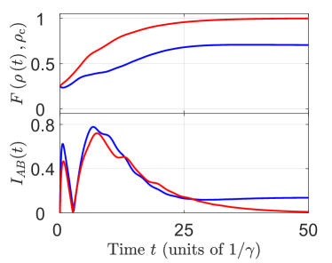
Figure 3: The time evolutions of the Uhlmann fidelity $F(\rho(t),\rho_{\mathrm{c}})$ and quantum mutual information $I_{AB}(t)$. The blue and red lines represent the driven systems under the quantum jump operators $L_{1}$ and $\widetilde{L}_{1}$, respectively. The system parameters are chosen as $\lambda/\gamma=0.5$ and $J_{ij}/\gamma=2$. The system is initially prepared in the state $|\Downarrow\rangle$ such that $F(\rho(0),\rho_{\mathrm{c}})=1/N$, where $N=4$ for simplicity. In the absence of modulation, the Uhlmann fidelity $F(\rho(t),\rho_{\mathrm{c}})$ (blue curve) saturates at approximately 0.75. On the other hand, the local dissipation channel $\widetilde{L}_{1}$ drives the system towards the state $\rho_{\mathrm{c}}$ with zero quantum mutual information $I_{AB}(t\rightarrow\infty)=0$. It is noteworthy that these conclusions hold irrespective of the system’s configuration and size.

In this section, we extend our main conclusion to a many-body quantum spin system based on the mechanism described above. In this case, the system is assumed to be described by a Heisenberg Hamiltonian under the influence of an external field. The Hamiltonian $H$ is defined as follows:

$$H = H_{\text{{spin}}}+H_{\mathrm{e}},$$ (6)

$$H_{\text{{spin}}} = -\sum_{i,j\neq i}(J_{ij}/2)\left(s_{i}^{+}s_{j}^{-}+s_{i}^{-}s_{j}^{+}\right)+\sum_{i,j\neq i}\Delta_{ij}s_{i}^{z}s_{j}^{z},$$

$$H_{\mathrm{e}} = \sum_{i}\lambda_{i}\mathbf{h}\cdot\mathbf{s}_{i}.$$ (7)

Here the operators $s_{i}^{\pm}=s_{i}^{x}\pm is_{i}^{y}$ and $s_{i}^{z}$ represent spin-$1/2$ operators at the $i$-th site, which obey the standard SU(2) symmetry relations: $[s_{i}^{z},s_{j}^{\pm}]=\pm s_{i}^{\pm}\delta_{ij}$ and $[s_{i}^{+},s_{j}^{-}]=2s_{i}^{z}\delta_{ij}$, where $\delta_{ij}$ is the Dirac delta function. The summation $\sum_{i,j\neq i}$ implies the summation over of possible pair interactions within an arbitrary range. The parameter $J_{ij}$ represents the inhomogeneous spin-spin interaction, while $\Delta_{ij}$ characterizes the anisotropy of the spin system $H_{\text{{spin}}}$. The local external field $\mathbf{h}=(1,0,0)$ can be interpreted as a magnetic field along the $x$-direction and is experimentally accessible in ultracold atom experiments Lee and Chan (2014); Ashida et al. (2017); Pan et al. (2019). The strength experienced by each spin is denoted as $\lambda_{i}$. When $\Delta_{ij}=J_{ij}/2$, the system $H_{\text{{spin}}}$ corresponds to a ferromagnetic Heisenberg Hamiltonian that respects the SU(2) symmetry, i.e., $[\sum_{i}s_{i}^{\sigma},H_{\text{{spin}}}]=0$ with $\sigma=\pm,z$. Thus, the eigenstates of $H_{\text{{spin}}}$ can be classified based on the total spin number $s$. Among these states, a fully polarized ferromagnetic state, denoted as $\left|\Uparrow\right\rangle=\prod\limits_{i=1}^{N}\left|\uparrow\right\rangle_{i}$ belongs to the ground states multiplet, where $|\uparrow\rangle_{i}\left(|\downarrow\rangle_{i}\right)$ is the eigenstate of $s_{i}^{z}$ with eigenenergy $\frac{1}{2}(-\frac{1}{2})$ Heisenberg (1928); Yang and Yang (1966). The degenerate ground states $\left\{\left|G_{n}\right\rangle\right\}$ belonging to the subspace $s=N/2$ are given by $\left|G_{n}\right\rangle=(\sum_{i}s_{i}^{-})^{n-1}\left|\Uparrow\right\rangle$, where $n$ ranges from $1$ to $N+1$. Clearly, $\left\{\left|G_{n}\right\rangle\right\}$ are the degenerate groundstates of $H_{\text{{spin}}}$ with an $(N+1)$-fold degeneracy, where all the spins are aligned in the same direction. However, the presence of the external field $H_{\mathrm{e}}$ breaks the SU(2) symmetry of the system, consequently splitting the degeneracy of these states. From this point onward, we will assume $\Delta_{ij}=J_{ij}/2$ for clarity.

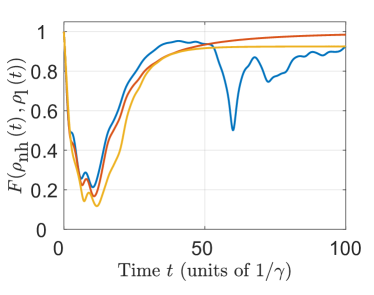
Figure 4: Plots of Uhlmann fidelity $F(\rho_{\text{{nh}}}\left(t\right),\rho_{\text{{l}}}\left(t\right))$ as a function of time $t$. Both $\rho_{\text{{nh}}}\left(t\right)$ and $\rho_{\text{{l}}}\left(t\right)$ are initialized in the state $\left|\Downarrow\right\rangle$ and driven by the effective non-Hermitian Hamiltonian $\mathcal{H}_{\mathrm{spin}}$ and $\mathcal{L}$. The blue, red, and yellow lines correspond to values of $\lambda/\gamma$ equal to $2/3$, $1/2$, and $1/4$, respectively. At $\lambda/\gamma=1/2$, which corresponds to the EP of $\mathcal{H}{\text{spin}}$, $F(\rho_{\text{{nh}}}\left(t\right),\rho_{\text{{l}}}\left(t\right))$ approaches $1$ since the coalescent state $\rho_{\mathrm{c}}$ is the final steady state for $\mathcal{L}$. For $\lambda/\gamma>1/2$, a full real spectrum of $\mathcal{H}_{\mathrm{spin}}$ emerges leading to the periodic evolution of $\rho_{\text{{nh}}}\left(t\right)$ without a definite direction in the Bloch sphere. This oscillatory behavior is represented by the blue line. When $\lambda/\gamma<1/2$, $\mathcal{H}{\text{spin}}$ exhibits imaginary energy levels, and the final steady state is determined by the maximum value among them. However, this state does not coincide with $\rho_{\text{l}}(t\rightarrow\infty)$ due to the different effects of the jump operator $L_{1}$ and $\mathcal{H}{\text{spin}}$. Consequently, $F(\rho_{\text{nh}}(t\rightarrow\infty),\rho_{\text{l}}(t\rightarrow\infty))<1$, indicating a deviation from unity. This can be observed in the plot represented by the yellow line.

The dissipation channels $L_{i}=s_{i}^{-}$ are now applied to all the local sites under the influence of a magnetic field. For simplicity, we will focus on the case where only a single lattice site is affected by the external field and dissipation channel. Specifically, we set $\lambda_{i}=\lambda\delta_{i,1}$ and $\Gamma_{\mu}=\gamma\delta_{\mu,1}$. The extension to multiple lattice sites is straightforward. Following Eq. (2), we can divide the dynamics into two parts: the first part involves the quantum jump operator that flips the spin on the first site from the up state $|\uparrow\rangle_{1}$ to the down state $|\downarrow\rangle_{1}$. Considering the external field as a perturbation, the low-energy excitation of the ferromagnetic Heisenberg model can be described by magnons. Intuitively, the collective behavior of spins leads to the spreading of the effect of $s_{1}^{-}$ across the entire system, ultimately resulting in the attainment of the final steady state $\left|\Downarrow\right\rangle$. The second part characterizes the non-unitary dynamics driven by the non-Hermitian spin Hamiltonian

$$\mathcal{H}_{\mathrm{spin}}=H-i\gamma s_{1}^{+}s_{1}^{-}/2.$$ (8)

Clearly, the local external field $H_{\mathrm{e}}=\lambda s_{1}^{x}$ and on-site dissipation channel $-i\gamma s_{1}^{+}s_{1}^{-}/2$ can be combined into a complex filed $H_{\mathrm{ec}}=\lambda s_{1}^{x}-i\gamma s_{1}^{+}s_{1}^{-}/2$ applied to the ferromagnetic Heisenberg Hamiltonian $H_{\text{{spin}}}$. In general, the commutation relation $[H_{\text{{spin}}},$ $H_{\mathrm{ec}}]\neq 0$ leads to a splitting of the ground state of $H_{\text{{spin}}}$ under the influence of $H_{\mathrm{ec}}$. However, when $\lambda\rightarrow\gamma/2$, the spliting approaches $0$, allowing us to treat $H_{\mathrm{ec}}$ as a non-Hermitian perturbation. To facilitate this treatment, we introduce the unitary transformation $U=\prod\nolimits_{j}U^{j}$ with $U^{j}=e^{-i\pi s_{j}^{x}/2}$, which represents a collective spin rotation along the $s^{x}$ direction by an angle $\pi/2$. The matrix form of $H_{\mathrm{ec}}$ in the degenerate subspace spanned by $\{|\widetilde{G}_{n}\rangle\}=\{U|G_{n}\rangle\}$ can be given as

$$W_{m,n} = \sqrt{\left(N+1-m\right)m}[\left(\lambda-\gamma/2\right)\delta_{m+1,n}$$ (9)

$$+\left(\lambda+\gamma/2\right)\delta_{m,n+1}]/2N.$$

Here, $W_{m,n}=\langle\widetilde{G}_{m}|UH_{\mathrm{ec}}U^{-1}|\widetilde{G}_{n}\rangle$. When $\lambda=\gamma/2$, it reduces to a Jordan block matrix with an EP of ($N+1$) order. The corresponding coalescent state with geometric multiplicity of $1$ is given as

$$|\widetilde{G}_{1}\rangle=\prod\nolimits_{j}|y,+\rangle_{j},$$ (10)

which represents all the spins aligning parallel to the $+y$ direction. These results are detailed and exemplified in the Appendix V.3. For an arbitrary initial state $\sum_{n}c_{n}\left(0\right)|\widetilde{G}_{n}\rangle$ within the subspace $s=N/2$, the coefficient $c_{m}\left(t\right)$ is given by the EP dynamics as

$$c_{m}\left(t\right) = c_{m}\left(0\right)+\sum_{n\neq m}\left(\frac{-it\lambda}{N}\right)^{m-n}\frac{h\left(m-n\right)}{\left(m-n\right)!}$$ (11)

$$\times[\prod\limits_{p=n+1}^{m}p\left(N+1-p\right)]^{1/2}c_{n}\left(0\right),$$

where $h\left(m-n\right)$ is the Heaviside step function (refer to Appendix V.3 for more details). The expression shows that the coefficient $c_{N+1}\left(t\right)$ of the evolved state always contains the highest power of time $t$. As a result, the component $c_{N+1}\left(t\right)$ dominates over the other components, leading to the final steady state being the coalescent state $|\psi_{\mathrm{c}}\rangle=e^{-i\frac{\pi}{2}s^{x}}\left|\Downarrow\right\rangle$ with $s^{x}=\sum_{i}s_{i}^{x}$. This implies that all spins align in parallel to the $y$-direction. We would like to emphasize that while our primary focus lies on the subspace indexed by $s=N/2$, the critical complex magnetic field resulting from local dissipation can also lead to the coalescence of eigenstates in each degenerate subspace with different quantum number $s$. Consequently, the coalescent states in each subspace have a geometric multiplicity of $1$. By following the EP$(N+1)$ dynamics in the $s=N/2$ subspace, an arbitrary initial state in a $s\neq N/2$ subspace evolves towards the corresponding coalescent state. If the initial state consists of multiple different types of coalescent states, then the final state is determined by the coalescent state whose time-dependent coefficient has the highest power of $t$.

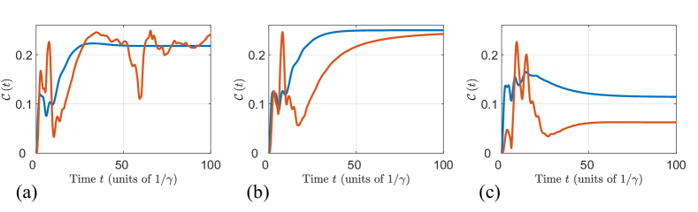
Figure 5: Time evolutions of the correlator $\mathcal{C}\left(t\right)$ for the evolved states $\rho_{\text{{l}}}\left(t\right)$ and $\rho_{\text{{nh}}}\left(t\right)$. The system parameters are set as follows: (a) $\lambda/\gamma=2/3$, (b) $\lambda/\gamma=1/2$, and (c) $\lambda/\gamma=1/4$. In each panel, the blue and red lines represent the $\mathcal{C}(t)$ driven by the Liouvillian superoperator $\mathcal{L}$ and the effective non-Hermitian Hamiltonian $\mathcal{H}_{\text{spin}}$, respectively. The correlator $\mathcal{C}\left(t\right)$ driven by $\mathcal{L}$ characterizes the spin-spin correlation of the NESS and asymptotically approaches a steady value over time. However, in the presence of an EP or imaginary energy levels in the Hamiltonian $\mathcal{H}_{\mathrm{spin}}$, the correlator $\mathcal{C}\left(t\right)$ converges to a specific asymptotic value instead of exhibiting indefinite oscillation. At the EP ($\lambda/\gamma=1/2$), both lines converge to the same value, $\mathcal{C}(t\rightarrow\infty)=1/4$, as shown in Fig. 4(b).

It can be imagined that the system will not approach the coalescent state $|\psi_{\mathrm{c}}\rangle$ under the effect of the Liouvillian superoperator $\mathcal{L}$ due to the distinct operations of two types of evolutions. To confirm this conjecture, we introduce Uhlmann fidelity Jozsa (1994) which measures the distance between density operators, defined by

$$F\left(\rho\left(t\right),\rho_{\mathrm{c}}\right)=(\text{{Tr}}\sqrt{\sqrt{\rho\left(t\right)}\rho_{\mathrm{c}}\sqrt{\rho\left(t\right)}})^{2}\text{,}$$ (12)

where $\rho_{\mathrm{c}}=|\psi_{\mathrm{c}}\rangle\langle\psi_{\mathrm{c}}|$ and $\rho\left(t\right)$ denotes the evolved density matrix. The system is initialized in the state $\left|\Downarrow\right\rangle$. The second physical quantity of interest is the quantum mutual information of the bipartite state $\rho_{AB}\left(t\right)$, which is defined as

$$I_{AB}=S\left(\rho_{A}\right)+S\left(\rho_{B}\right)-S\left(\rho_{AB}\right),$$ (13)

where $S\left(\rho_{\sigma}\right)=-$Tr$\rho_{\sigma}$ln$\rho_{\sigma}$ ($\sigma=A,B$) represents the Von Neumann entropy of $\rho_{\sigma}\left(t\right)$. This entropy is obtained by tracing out system $B$ or $A$ from the joint density matrix $\rho_{AB}$. More specifically, $\rho_{A}\left(t\right)=$Tr${}_{B}[\rho_{AB}\left(t\right)]$ or $\rho_{B}\left(t\right)=$Tr${}_{A}[\rho_{AB}\left(t\right)]$. $S\left(\rho_{AB}\right)$ denotes the Von Neumann entropy of the total state. The quantity $I_{AB}$ is formally equivalent to the classical mutual information, with the Shannon entropy replaced by its quantum counterpart. Utilizing $I_{AB}$, we can effectively capture the separability of the evolved state. If $I_{AB}=0$, the evolved state $\rho_{AB}\left(t\right)$ is considered simply separable or a product state. In our system, we divide it into two parts: part $A$ consists of a single local spin, while part $B$ represents its complement. When the NESS assumes a product form, $I_{AB}$ will be $0$. In Fig. 3, we conduct a numerical simulation on these two quantities. The results indicate that $F\left(\rho\left(t\right),\rho_{\mathrm{c}}\right)$ initially increases during the short-time evolution, as it is determined by the non-Hermitian Hamiltonian $\mathcal{H}_{\mathrm{spin}}$, which drives $\rho\left(t\right)$ towards $\rho_{\mathrm{c}}$. However, as the long-time evolution progresses, a compromise between two distinct types of probabilistic evolution emerges, leading to a deviation of the NESS from $\rho_{\mathrm{c}}$. Additionally, we observe that the minimum value of $I_{AB}$ is approximately $0.136$, implying that the spin at the first site remains correlated with the other component. Consequently, the evolved state $\rho(t)$ is not a product state.

To recover the final state $|\psi_{\mathrm{c}}\rangle$, one should introduce a unitary operator $U=e^{-i\frac{\pi}{2}s^{x}}$ to the quantum jump operator

$$\widetilde{L}_{1}=Us_{1}^{-}=\left(s_{1}^{x}-is_{1}^{z}\right)U.$$ (14)

The operator $\widetilde{L}$ performs two operations: firstly, it rotates the spin by an angle of $\pi/2$ along the $x$-direction, and secondly, it projects the spin at the first site onto the $y$-direction, resulting in the state $|y_{1},+\rangle$. The unitary operation $U=e^{-i\frac{\pi}{2}s^{x}}$ does not affect non-Hermitian Hamiltonian $\mathcal{H}_{\mathrm{spin}}$ since $\widetilde{L}_{1}^{\dagger}\widetilde{L}_{1}=L_{1}^{\dagger}L_{1}$. Its effect is limited to the quantum trajectories that deviate from the post-selected no-click trajectory. However, the effect of $\widetilde{L}_{1}$ on the first spin is equivalent to that of $\mathcal{H}_{\mathrm{spin}}$ which tends to freeze each spin along $y$-direction. As a result, regardless of the type of probabilistic evolution in each quantum trajectory, the long-term tendency leads to the same consequence, suggesting that $\rho_{\mathrm{NESS}}=|\psi_{\mathrm{c}}\rangle\langle\psi_{\mathrm{c}}|$ represents the NESS of the open quantum spin system. In the Appendix V.4, we verify that $\rho_{\mathrm{NESS}}$ is indeed the eigenfunction of the Liouvillian superoperator $\mathcal{L}$ with zero energy. Consequently, $\mathcal{H}_{\mathrm{spin}}$ and $\mathcal{L}$ share the same steady state within the subspace $\left\{\left|G_{n}\right\rangle\right\}$. This is further confirmed in Fig. 3, where the Uhlmann fidelity $F\left(\rho\left(t\right),\rho_{\mathrm{c}}\right)\rightarrow 1$ and $I_{AB}\left(t\right)\rightarrow 0$ correspond to the final product state of $|\psi_{\mathrm{c}}\rangle$. Furthermore, we compare the evolution of two density matrices driven by $\mathcal{H}_{\mathrm{spin}}$ and $\mathcal{L}$, at $\lambda=\gamma/2$, respectively. The initial state is $\left|\Downarrow\right\rangle$, prepared within the subspace $\left\{\left|G_{n}\right\rangle\right\}$. We examine the Uhlmann fidelity between the two evolved states $\rho_{\text{{nh}}}\left(t\right)$ and $\rho_{\text{{l}}}\left(t\right)$ as depicted in Fig. 4, where $\rho_{\text{{nh}}}\left(t\right)=e^{-i\mathcal{H}_{\mathrm{spin}}t}\rho_{\text{{nh}}}\left(0\right)e^{i\mathcal{H}_{\mathrm{spin}}^{\dagger}t}$ and $\rho_{\text{{l}}}\left(t\right)=e^{\mathcal{L}t}\rho_{\text{{l}}}\left(0\right)$. The two states $\rho_{\text{{nh}}}\left(0\right)$ and $\rho_{\text{{l}}}\left(0\right)$ are initialized in the state $\left|\Downarrow\right\rangle$. The fidelity initially decreases and then rapidly increases to $1$, indicating that the long-time dynamics of $\rho\left(t\right)$ driven by $\mathcal{L}$ can be effectively described by $\mathcal{H}_{\mathrm{spin}}$. To gain further insight into the two types of the evolution, we also investigate the time evolution of the correlator $\mathcal{C}\left(t\right)=\mathrm{Tr}[\rho\left(t\right)s_{1}^{+}s_{N}^{-}]$ for two such evolved states. In Fig. 5(b), the two curves exhibit the same long-time tendency and finally approaches $\mathcal{C}\left(t\right)=0.25$ when $\lambda/\gamma=1/2$, which can be also captured by the Uhlmann fidelity. This result is quite astonishing as it challenges the common belief that $\mathcal{H}_{\mathrm{spin}}$ captures the short-time dynamics before a quantum jump occurs, while $\mathcal{L}$ characterizes the long-time dynamics. Before ending this discussion, it is worth noting that when the initial state is prepared in a different degenerate subspace ($s\neq N/2$), the final evolved state becomes an entangled state rather than a separable state where all the spins align in the same direction, as observed in the $s=N/2$ subspace. Achieving collective magnetization requires careful modulation of the quantum jump operator $\mathcal{L}$ to align its action with the effect of $\mathcal{H}_{\mathrm{spin}}$. This process may involve multiple dissipation channels and present significant challenges in both theoretical and experimental aspects. Consequently, our proposal is specifically applicable to the $s=N/2$ subspace.

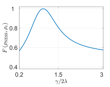
Figure 6: Plot of $F\left(\rho_{\mathrm{NESS}},\rho_{\mathrm{c}}\right)$ as a function of $\gamma$. The strength of the external field is fixed at $\lambda=0.5$. The configuration of the system is shown in Fig. 1. Notably, a peak is observed at $\gamma=2\lambda$, which corresponds to the EP of the effective non-Hermitian Hamiltonian $\mathcal{H}_{\mathrm{spin}}$. It is worth mentioning that slight deviations from $1$ do not significantly impact the NESS. This observation indicates the existence of a parameter window that allows for magnetization induced by local dissipation.

Now let us further investigate whether this conclusion holds when the system parameters are not finely tuned. First, we consider the case where $\gamma$ deviates from $\gamma_{c}=\lambda/2$. We plot Fig. 6, which shows $F\left(\rho\left(t\rightarrow\infty\right),\rho_{\mathrm{c}}\right)$ as a function of $\gamma$. It can be observed that the final steady state is almost unaffected as $\gamma$ deviates slightly from $\gamma_{c}$. However, when $\gamma\ll\gamma_{c}$, there are no EP and complex energy in $\mathcal{H}_{\mathrm{spin}}$. In this case, the state initialized in the subspace $\left\{\left|G_{n}\right\rangle\right\}$ will not tend to a definite state but instead oscillates between different eigenenergies, resulting in a periodic oscillation of the physical observables. This can be seen from the Fig. 5(a). Consequently, the density matrix driven by $\mathcal{H}_{\mathrm{spin}}$ will exhibit distinct dynamics from the quantum jump operator which forces the spin along the $y$-direction. Combining both effects, the NESS deviates from $\rho_{\mathrm{c}}$. On the other hand, when $\gamma\gg\gamma_{c}$, $\mathcal{H}_{\mathrm{spin}}$ drives all the spins to the down states since the eigenstate $\left|\Downarrow\right\rangle$ has the largest imaginary part. However, this contradicts the action of the quantum jump operator. As a consequence of the parameter deviation, the final state is no longer a product state with a definite direction but a mixed state that loses some of its coherence.

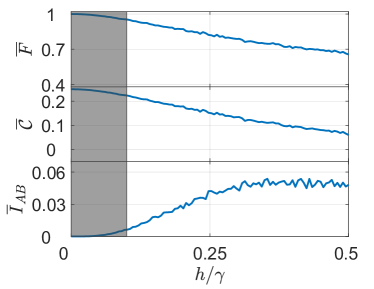
Figure 7: Numerical simulations of $\overline{F}\left(\rho_{\mathrm{NESS}},\rho_{\mathrm{c}}\right)$, $\overline{\mathcal{C}}\left(t\rightarrow\infty\right)$, and $\overline{I}_{AB}\left(t\rightarrow\infty\right)$ as functions of the disorder strength $h$. The system parameters are fixed at $\lambda/\gamma=0.5$, and $J_{ij}/\gamma=1$. The structure of the system is depicted in Fig. 1. The average Uhlmann fidelity $\overline{F}\left(\rho_{\mathrm{NESS}},\rho_{\mathrm{c}}\right)$, average correlator $\overline{\mathcal{C}}\left(t\rightarrow\infty\right)$, and average quantum mutual information $\overline{I}_{AB}\left(t\rightarrow\infty\right)$ are calculated by averaging over 1000 disorder configurations. The simulations demonstrated that the realization of $\rho_{\mathrm{c}}$ remains unaffected by the specific system configuration and is immune to weak disorder, as indicated by the gray shaded region. This property is advantageous for observing the magnetization induced by single local dissipation in experimental setups.

Besides the deviation from the EP, another factor influencing the success of the scheme is the presence of disorder. In the experiment, our proposal can be realized in a cold atom system, particularly in the Rydberg atom quantum simulator. Smith et al. (2016); Zhang et al. (2017); Marcuzzi et al. (2017); Shibata et al. (2020); Mondragon-Shem et al. (2021) The system can be subjected to disorder through external fields, such as electric or magnetic fields. Fluctuations or variations in the strength and direction of these fields can impact the energy levels and dynamics. It is crucial to examine the system’s robustness to disorder. To achieve this, we introduce disorder by considering a random magnetic field in the $z$ direction. The modified system Hamiltonian is given as

$$H_{\text{{spin}}}^{\mathrm{d}}=H_{\text{{spin}}}+H^{\mathrm{d}},$$ (15)

with

$$H^{\mathrm{d}}=\sum_{i}h_{i}s_{i}^{z},$$ (16)

where $h_{i}$ represents a random number within the range $(-h,$ $h)$. Clearly, $H^{\mathrm{d}}$ breaks the SU(2) symmetry of $H_{\text{{spin}}}^{\mathrm{d}}$ and hence prevents the formation of the subpace of $\left\{\left|G_{n}\right\rangle\right\}$. Although exact SU(2) symmetry is spoiled, it can be inferred that the directed evolution in the $\left\{\left|G_{n}\right\rangle\right\}$ subspace may still exist under weak disorder. In Fig. 7, we perform the numerical simulation to examine the average Uhlmann fidelity $\overline{F}\left(\rho_{\mathrm{NESS}},\rho_{\mathrm{c}}\right)$, average correlator $\overline{\mathcal{C}}\left(t\rightarrow\infty\right)$ and average quantum mutual information $\overline{I}_{AB}\left(t\rightarrow\infty\right)$. The results demonstrate that a small distribution of $h$ does not induce a transition in the final state as the degenerate subspace $\left\{\left|G_{n}\right\rangle\right\}$ is approximately preserved, as manifested by the behavior of $\overline{\mathcal{C}}\left(t\rightarrow\infty\right)$ and $\overline{I}_{AB}\left(t\rightarrow\infty\right)$ in the grey shaded region. However, when $h$ is large enough to completely destroy the SU(2) symmetry, the dynamics of EP cannot be maintained as the degenerate subspace ceases to exist. In such a scenario, the action of $\mathcal{H}_{\mathrm{spin}}$ and the quantum jump operator $\widetilde{L}$ exhibit distinct dynamics, leading to the collapse of the final ferromagnetic state.

IV Summary

In conclusion, we have demonstrated that the critical non-Hermitian system accurately captures the long-term dynamics of the open quantum system. Specifically, the master equation of the open quantum system can be rephrased as a stochastic average over individual trajectories, which can be numerically evolved as pure states over time. Each trajectory’s evolution is determined by the SSE. There are two types of probabilistic evolution: a non-unitary evolution driven by the effective non-Hermitian Hamiltonian and a state projection determined by the quantum jump operator. The trade-off between these two evolutions determines the final NESS. For the non-Hermitian Hamiltonian, a definite final evolved state can be achieved if the system possesses the EP or an imaginary energy level. In the former case, the evolved state is forced towards the coalescent state, while in the latter case, it approaches the eigenstate with the maximum value of the imaginary energy level. If the final evolved state coincides with the state under the quantum jump operation, then the NESS of the open quantum system is identical to the coalescent state of the effective non-Hermitian Hamiltonian. Furthermore, we apply this mechanism to the open quantum spin system and find that local critical dissipation can induce a high-order EP in the effective non-Hermitian ferromagnetic Heisenberg system. The dimension of the degenerate subspace determines the order of the EP. The corresponding coalescent state represents all the spins aligned in parallel to the $y$-direction. From a dynamical perspective, when the initial state is prepared within the degenerate subspace, the EP dynamics force all the spins to align in the y-direction regardless of the initial spin configuration. On the other hand, the quantum jump operator rotates the spin that passes the first site to align with the direction of the coalescent state. Both actions of the two probabilistic propagations are identical, leading to the NESS being the coalescent state. The realization of this type of NESS is immune to weak disorder and holds within a certain range of system parameters. These findings serve as the building blocks for understanding critical open quantum systems from both theoretical and experimental perspectives.

V Appendix

V.1 EP dynamics of two-level system

In this subsection, we analyze the EP dynamics in a non-Hermitian two-level system. The Hamiltonian, given by

$$\mathcal{H}=\lambda s^{x}-\frac{i\gamma}{2}s^{+}s^{-},$$ (17)

is non-Hermitian due to the dissipation channel. In the basis of $\{|\uparrow\rangle,$ $|\downarrow\rangle\}$, the matrix form of $\mathcal{H}$ is expressed as

$$\mathcal{H}=\frac{1}{2}\left(\begin{array}[]{cc}-i\gamma/2&\lambda\\ \lambda&i\gamma/2\end{array}\right)-\frac{i\gamma}{4}I,$$ (18)

where $\frac{i\gamma}{4}I$ is a constant term that does not affect the relative probability of populating the two different energy states. The two eigenstates of $\mathcal{H}$ coalesce at the EP when $\lambda=\gamma/2$. The corresponding coalescent state is $|\psi_{\mathrm{c}}\rangle=|y,+\rangle=\frac{1}{\sqrt{2}}\left(1,\text{ }i\right)^{T}$ which also represents the eigenstate of $s^{y}$ with eigenenergy $1/2$. Now, let us turn focus on the system propagator $\mathcal{U}_{2}$. Due to the nilpotent matrix property of $\mathcal{H}$, i.e., $\mathcal{H}^{2}=0$, $\mathcal{U}_{2}$ simplifies to

$$\mathcal{U}_{2}=e^{-i\mathcal{H}t}=e^{-\gamma t/4}\left[1-\frac{i\lambda t}{2}\left(\begin{array}[]{cc}-i&1\\ 1&i\end{array}\right)\right].$$ (19)

For an arbitrary initial state $|\psi\left(0\right)\rangle=\left(a,\text{ }b\right)^{T}$, the evolved state can be given as

$$|\psi\left(t\right)\rangle=e^{-\gamma t/4}\left(\begin{array}[]{c}a-i\lambda t/2\\ b+\lambda t/2\end{array}\right),$$ (20)

As time tends to infinity, $|\psi\left(t\right)\rangle$ normalized in terms of Dirac probability approaches $|\psi\left(\infty\right)\rangle=|\psi_{\mathrm{c}}\rangle$.

V.2 NESS of an open two-level system

In this subsection, we derive the NESS of the two-level open system under consideration. The LME describing the open system dynamics is given by

$$\frac{\text{{d}}\rho}{\text{{d}}t}=-i\lambda[s^{x},\rho]-\frac{\gamma}{2}\left(s^{+}s^{-}\rho+\rho s^{+}s^{-}\right)+\gamma s^{-}\rho s^{+}.$$ (21)

By applying the Choi-Jamiołkowski isomorphism, the LME can be written as an equivalent form:

$$\frac{\text{{d}}\rho}{\text{{d}}t}\equiv\widetilde{\mathcal{L}}\rho,$$ (22)

where the vectorized density matrix $|\rho\rangle=\sum_{m,n}\rho_{m,n}|m\rangle\otimes|n\rangle$ represents the density matrix in the double space. The Liouvillian superoperator is given by

$$\widetilde{\mathcal{L}} = -i\lambda\left(s^{x}\otimes I-I\otimes s^{x}\right)+\gamma s^{-}\otimes s^{-}$$ (23)

$$-\frac{\gamma}{2}\left(s^{+}s^{-}\otimes I+I\otimes s^{+}s^{-}\right).$$

The matrix representation of $\widetilde{\mathcal{L}}$ can be expressed as

$$\widetilde{\mathcal{L}}=\left(\begin{array}[]{cccc}-\gamma&i\frac{\lambda}{2}&-i\frac{\lambda}{2}&0\\ i\frac{\lambda}{2}&-\frac{1}{2}\gamma&0&-i\frac{\lambda}{2}\\ -i\frac{\lambda}{2}&0&-\frac{1}{2}\gamma&i\frac{\lambda}{2}\\ \gamma&-i\frac{\lambda}{2}&i\frac{\lambda}{2}&0\end{array}\right).$$ (24)

The complete spectrum of the Liouvillian superoperator $\mathcal{L}$ can be obtained by solving the eigen-equation: $\widetilde{\mathcal{L}}|\rho_{k}\rangle=\varepsilon_{k}|\rho_{k}\rangle$, where $k$ represents the eigenvalue and $|\rho_{k}\rangle$ denotes its corresponding eigenmatrix. The NESS is unique and corresponds to the eigenvalue $\varepsilon_{k}=0$. Straightforward algebra reveals that the corresponding eigenmatrix is given by

$$\rho_{\mathrm{NESS}}=\left(\begin{array}[]{cc}\frac{\lambda^{2}}{2\lambda^{2}+\gamma^{2}}&-i\frac{\lambda\gamma}{2\lambda^{2}+\gamma^{2}}\\ i\frac{\lambda\gamma}{2\lambda^{2}+\gamma^{2}}&\frac{\lambda^{2}+\gamma^{2}}{2\lambda^{2}+\gamma^{2}}\end{array}\right).$$ (25)

V.3 Non-Hermitian Heisenberg model and EP dynamics

V.3.1 model and EP

In this subsection, we analyze the non-Hermitian Heisenberg model with a local dissipation channel and identify the EP. According to the main text, the Hamiltonian of the effective non-Hermitian Heisenberg model in the LME under an external field is given by

$$\mathcal{H}_{\mathrm{spin}}=H_{\mathrm{spin}}+H_{\mathrm{ec}},$$ (26)

where

$$H_{\mathrm{spin}}=-\frac{1}{2}\sum_{i,j\neq i}J_{ij}(s_{i}^{+}s_{j}^{-}+s_{i}^{-}s_{j}^{+}+2s_{i}^{z}s_{j}^{z}),$$ (27)

and

$$H_{\mathrm{ec}}=\sum_{\left\{i\right\}}\lambda_{i}\mathbf{h}\cdot\mathbf{s}_{i}-\frac{i}{2}\sum_{i}\Gamma_{i}s_{i}^{+}s_{i}^{-}.$$ (28)

$H_{\mathrm{ec}}$ can be deemed as the external complex magnetic filed. Here, $\left\{i\right\}$ represents a set of multiple local sites that are subjected to the local complex fields. The presence of inhomogeneous magnetic fields breaks the $SU(2)$ symmetry, i.e., $\left[s^{\pm},\mathcal{H}_{\mathrm{spin}}\right]\neq 0$. However, $H_{\mathrm{spin}}$ and $H_{\mathrm{ec}}$, commute with each other when the homogeneous magnetic field and dissipation are applied, i.e., $\lambda_{i}=\lambda$ and $\Gamma_{i}=\gamma$. Although these Hamiltonians share common eigenstates, the properties of the ground states are unclear due to the non-Hermitian nature of $H_{\mathrm{ec}}$. This poses a challenge to perturbation theory in Hermitian quantum mechanics since the omission of high-order corrections cannot be guaranteed in the complex regime. To simplify the analysis, we consider $\lambda_{i}=\lambda\delta_{i,1}$, and $\Gamma_{i}=\gamma\delta_{i,1}$ from this point onwards. To proceed, we introduce a similarity transformation $\mathcal{S}_{1}=\prod\nolimits_{j}\mathcal{S}_{1}^{j}$, where $\mathcal{S}_{1}^{j}=e^{-i\theta s_{j}^{y}}$ represents a counter-clockwise spin rotation in the $s_{x}$-$s_{z}$ plane around the $s_{y}$-axis by an angle $\theta$. Here $\theta$ is a complex number dependent on the strength of the complex field, given by $\theta=\tan^{-1}\left(2\lambda/i\gamma\right)$. It is important to note that the spin rotation $\mathcal{S}_{1}^{j}$ is valid at arbitrary $\gamma$ except at EP of $H_{\mathrm{ec}}$ ($\lambda=\gamma/2$), where $H_{\mathrm{ec}}$ takes a non-diagonalizable Jordan block form. Under the spin-rotation, the transformed Hamiltonian is as follows:

$$\overline{\mathcal{H}}_{\mathrm{spin}} = \overline{H}_{\mathrm{spin}}+\overline{H}_{\mathrm{ec}},$$ (29)

$$\overline{H}_{\mathrm{spin}} = -\frac{1}{2}\sum_{i,j\neq i}J_{ij}(\tau_{i}^{+}\tau_{j}^{-}+\tau_{i}^{-}\tau_{j}^{+}+2\tau_{i}^{z}\tau_{j}^{z}),$$ (30)

$$\overline{H}_{\mathrm{ec}} = \sqrt{\lambda^{2}-\gamma^{2}/4}\tau_{1}^{z}-\frac{i\gamma}{4},$$ (31)

where the new set of operators $\tau_{j}^{\pm}=(\mathcal{S}_{1}^{j})^{-1}s_{j}^{\pm}\mathcal{S}_{1}^{j}$ and $\tau_{j}^{z}=(\mathcal{S}_{1}^{j})^{-1}s_{j}^{z}\mathcal{S}_{1}^{j}$ also satisfies the Lie algebra. We omit the overall decay factor $-i\gamma/4$ which served as the energy base has no effects on the subsequent evolution. Specifically, they obey the commutation relations $[\tau_{i}^{z},\tau_{j}^{\pm}]=\pm\tau_{i}^{\pm}\delta_{ij}$ and $[\tau_{i}^{+},\tau_{j}^{-}]=2\tau_{i}^{z}\delta_{ij}$. It is important to note that $\tau_{j}^{\pm}\neq(\tau_{j}^{\mp})^{\dagger}$ due to the complex rotation angle $\theta$. We consider the eigenstates of the operator $\sum_{i}s_{i}^{z}$, denoted as $\left\{\left|\psi_{n}\right\rangle\right\}$, which represent possible spin configurations along the $+z$ direction. Under the biorthogonal basis of $\{\mathcal{S}^{-1}\left|\psi_{n}\right\rangle\}$ and $\{\mathcal{S}^{\dagger}\left|\psi_{n}\right\rangle\}$, the matrix form of $\overline{\mathcal{H}}_{\mathrm{spin}}$ is Hermitian for $\lambda>\gamma/2$ except a complex energy base. Although the presence of the local complex field breaks the SU(2) symmetry of the system, as indicated by $[\overline{H}_{\mathrm{ec}},$ $\overline{\mathcal{H}}_{\mathrm{spin}}]\neq 0$, the entirely real spectrum remains without symmetry protection. When $\lambda=\gamma/2$, the transformation of $\mathcal{S}_{1}$ is ill-defined, indicating that $H_{\mathrm{ec}}$ is non-diagonalizable, which corresponds to the presence of an EP. In principle, the EP of $\mathcal{H}_{\mathrm{spin}}$ or $\overline{\mathcal{H}}_{\mathrm{spin}}$ may not coincide with the EP of $H_{\mathrm{ec}}$ at $\lambda=\gamma/2$. In the following, we will demonstrate that $\mathcal{H}_{\mathrm{spin}}$ and $H_{\mathrm{ec}}$ exhibit the same EP behavior within the framework of perturbation theory.

The Hermiticity of the matrix representation of $\overline{\mathcal{H}}_{\mathrm{spin}}$ allows us to apply various approximation methods in quantum mechanics. As$\ \gamma$ approaches $2\lambda$, the value of $\sqrt{\lambda^{2}-\gamma^{2}/4}$ becomes small, allowing $\overline{H}_{\mathrm{ec}}$ in the new frame to be treated as a weak perturbation. Our focus is on the influence of $\overline{H}_{\mathrm{ec}}$ on the ground states $\left\{\left|G_{n}^{\prime}\right\rangle\right\}$ of $\overline{H}_{\mathrm{spin}}$. Due to the properties of the ferromagnetic spin system $\overline{H}_{\mathrm{spin}}$, the ground states $\left\{\left|G_{n}^{\prime}\right\rangle\right\}$ exhibit $(N+1)$ fold-degeneracy and can be expressed as

$$\left|G_{n}^{\prime}\right\rangle=(\sum_{i}\tau_{i}^{-})^{n-1}\left|\Uparrow\right\rangle^{\prime}\text{ }\left(n=1,\text{ }2\text{ }...\text{ }N+1\right)\text{, }$$ (32)

where

$$\left|\Uparrow\right\rangle^{\prime}=(\mathcal{S}_{1})^{-1}\left|\Uparrow\right\rangle\text{, and }\left|\Uparrow\right\rangle=\prod\limits_{i=1}^{N}\left|\uparrow\right\rangle_{i}\text{.}$$ (33)

$\left|G_{n}^{\prime}\right\rangle$ is also the eigenstate of $\mathbf{\tau}^{2}=\sum_{i}\mathbf{\tau}_{i}^{2}$ with $\tau=N/2$, where $N$ denotes the total number of spins. Noticeably, the presence of degenerate ground states is irrelevant to the system’s structure. This property can be observed in other types of systems as well Heisenberg (1928); Yang and Yang (1966). Following the principles of degenerate perturbation theory, the eigenvalues up to first order can be determined by the matrix representation of $\overline{H}_{\mathrm{ec}}$ within the subspace spanned by $\left\{\left|G_{n}^{\prime}\right\rangle\right\}$. For simplicity, we refer to the corresponding perturbed matrix as $W^{\prime}$, with elements given by $W_{m,n}^{\prime}=\langle\overline{G}_{m}^{\prime}|\overline{H}_{\mathrm{ec}}|G_{n}^{\prime}\rangle$. The biorthogonal left eigenvectors are denoted as $\{\langle\overline{G}_{m}^{\prime}|\}$ and can be expressed as

$$\langle\overline{G}_{m}^{\prime}|=\left\langle\Uparrow\right|\mathcal{S}_{1}(\sum_{i}\tau_{i}^{+})^{m-1}\text{ }\left(m=1,\text{ }2\text{ }...\text{ }N+1\right).$$ (34)

Two important points are highlighted: (i) Owing to the Hermiticity of the matrix $W^{\prime}$, higher-order corrections can be safely disregarded as$\ \gamma$ approaches $2\lambda$. (ii) When a homogeneous magnetic field is applied, $\left[\overline{H}_{\mathrm{ec}},\text{ }\overline{\mathcal{H}}_{\mathrm{spin}}\right]=0$, enabling the decomposition of $\overline{\mathcal{H}}_{\mathrm{spin}}$ into block matrices based on the eigenvectors of $\mathbf{\tau}^{2}$. Consequently, the eigenvalues of $W^{\prime}$ comprise the energies of the ground state and $N$ excited states of $\overline{\mathcal{H}}_{\mathrm{spin}}$. After straightforward algebras, the entry of the matrix can be obtained as

$$\ W_{m,n}^{\prime}=\sqrt{\lambda^{2}-\gamma^{2}/4}[\left(N/2-m+1\right)\delta_{m,n}]/N,$$ (35)

where the factor $1/N$ arises from the translation symmetry of the ground state $\{\left|G_{n}\right\rangle^{\prime}\}$. By performing the transformation $W=U\mathcal{S}_{1}W^{\prime}(\mathcal{S}_{1})^{-1}U^{-1}$ ($W_{m,n}=\langle\widetilde{G}_{m}|UH_{\mathrm{ec}}U^{-1}|\widetilde{G}_{n}\rangle$ with $|\widetilde{G}_{n}\rangle=U\left|G_{n}\right\rangle$), the matrix element of $W$ can be expressed as

$$W_{m,n} = \sqrt{\left(N+1-m\right)m}[\left(\lambda-\gamma/2\right)\delta_{m+1,n}$$ (36)

$$+\left(\lambda+\gamma/2\right)\delta_{m,n+1}]/2N.$$

When $\lambda=\gamma/2$, it reduces to a Jordan block form, and an EP of order $N+1$ occurs. The corresponding coalsecent is $|\psi_{\mathrm{c}}\rangle=\prod\nolimits_{j}e^{-i\frac{\pi}{2}s_{j}^{x}}\left|\Downarrow\right\rangle$. It is worth mentioning that if we express $H_{\mathrm{ec}}$ in the basis of $\left\{\left|G_{n}\right\rangle\right\}$, it describes a $\mathcal{PT}$-symmetric hypercube graph of $N+1$ dimension Zhang et al. (2012). The EP also emerges when $\lambda=\gamma/2$.

V.3.2 high order EP dynamics

In this subsection, our objective is to generate a saturated ferromagnetic state where all local spins (or conduction electron spins) are aligned parallel to the $y$-direction. The non-Hermitian Heisenberg Hamiltonian is represented by Eq. (8) in the main text. Considering the EP $\lambda=\gamma/2$ within the subspace $\{|\widetilde{G}_{n}\rangle\}$, the matrix form of $W$ can be expressed as

$$W_{m,n}=\lambda\sqrt{\left(N+1-m\right)m}\delta_{m,n+1}/N,$$ (37)

which corresponds to a Jordan block of dimension $N+1$. The coalescent eigenstate is $|\widetilde{G}_{N+1}\rangle$. It is important to note that $W$ is a nilpotent matrix with order $\left(N+1\right)$ meaning that $\left(W\right)^{N+1}=0$. The element of matrix $W^{k}$ can be given as

$$\left(W^{k}\right)_{mn}=[\prod\limits_{p=m+1-k}^{m}p\left(N+1-p\right)]^{1/2}(\frac{\lambda}{N})^{k}\delta_{m,n+k},$$ (38)

where $k<m+1$. Our attention now shifts to the dynamics of the critical matrix $W$, and the evolution of states within this subspace is governed by the propagator $\mathcal{U=}e^{-iWt}$. Utilizing Eq. (38), we can derive the elements of the propagator $\mathcal{U}$ as follows:

$$\mathcal{U}_{m,n} = \delta_{mn}+\left(\frac{-it\lambda}{N}\right)^{m-n}\frac{h\left(m-n\right)}{\left(m-n\right)!}$$ (39)

$$\times[\prod\limits_{p=n+1}^{m}p\left(N+1-p\right)]^{1/2},$$

where $h\left(x\right)$ is a step function defined as $h\left(x\right)=1$ $\left(x>0\right),$ and $h\left(x\right)=0$ $\left(x<0\right)$. Considering an arbitrary initial state $\sum_{n}c_{n}\left(0\right)|\widetilde{G}_{n}\rangle$, the coefficient $c_{m}\left(t\right)$ of the evolved state is given by

$$c_{m}\left(t\right) = c_{m}\left(0\right)+\sum_{n\neq m}\left(\frac{-it\lambda}{N}\right)^{m-n}\frac{h\left(m-n\right)}{\left(m-n\right)!}$$ (40)

$$\times[\prod\limits_{p=n+1}^{m}p\left(N+1-p\right)]^{1/2}c_{n}\left(0\right).$$

It is evident that regardless of the initial state chosen, the coefficient $c_{N+1}\left(t\right)$ of evolved state always contains the highest power of time $t$. As time progresses, the component $c_{N+1}\left(t\right)$ of the evolved state overwhelms the other components, ensuring the final state is coalescent state $|\psi_{\mathrm{c}}\rangle=\prod\nolimits_{j}e^{-i\frac{\pi}{2}s_{j}^{x}}\left|\Downarrow\right\rangle$ under the Dirac normalization. The different types of initial states only determine how the total probability of the evolved state increases over time and the relaxation time for it to evolve towards the coalescent state.

V.4 NESS of the open quantum spin system subjected to a local magnetic field

In this subsection, we demonstrate that the critical density matrix $\rho_{\mathrm{c}}=|\psi_{\mathrm{c}}\rangle\langle\psi_{\mathrm{c}}|$ is also the NESS of the open quantum spin system. The dynamics of the open quantum spin system under consideration is governed by LME, expressed as:

$$\frac{\text{{d}}\rho}{\text{{d}}t} = -i(\mathcal{H}_{\mathrm{spin}}\rho-\rho\mathcal{H}_{\mathrm{spin}}^{\dagger})$$ (41)

$$+\gamma\left(s_{1}^{x}-is_{1}^{z}\right)U\rho U^{-1}\left(s_{1}^{x}+is_{1}^{z}\right)$$

$$\equiv \mathcal{L}\rho,$$

where $U$ is defined as the product of operators $U=\prod\nolimits_{j}e^{-i\pi s_{j}^{x}/2}$ and

$$\mathcal{H}_{\mathrm{spin}} = H_{\mathrm{spin}}+H_{\mathrm{ec}},$$ (42)

$$H_{\mathrm{spin}} = -\frac{1}{2}\sum_{i,j\neq i}J_{ij}(s_{i}^{+}s_{j}^{-}+s_{i}^{-}s_{j}^{+}+2s_{i}^{z}s_{j}^{z}),$$ (43)

$$H_{\mathrm{ec}} = \lambda s_{1}^{x}-\frac{i\gamma}{2}s_{1}^{+}s_{1}^{-},$$ (44)

Here $\lambda=\gamma/2$ is assumed when $\mathcal{H}_{\mathrm{spin}}$ is at EP. Next, we substitute $\rho_{\mathrm{c}}=|\psi_{\mathrm{c}}\rangle\langle\psi_{\mathrm{c}}|$ into the above equation. Recalling that the $|\psi_{\mathrm{c}}\rangle=\prod\nolimits_{j}e^{-i\frac{\pi}{2}s_{j}^{x}}\left|\Downarrow\right\rangle$, we can readily deduce that $\mathcal{H}_{\mathrm{spin}}|\psi_{\mathrm{c}}\rangle=-i\gamma/4|\psi_{\mathrm{c}}\rangle$, resulting in

$$-i(\mathcal{H}_{\mathrm{spin}}\rho_{\mathrm{c}}-\rho_{\mathrm{c}}\mathcal{H}_{\mathrm{spin}}^{\dagger})=-\frac{\gamma}{2}\rho_{\mathrm{c}}.$$ (45)

Applying $\left(s_{1}^{x}-is_{1}^{z}\right)U$ to $|\psi_{\mathrm{c}}\rangle$ yields $\frac{1}{\sqrt{2}}|\psi_{\mathrm{c}}\rangle$. Thus, we can conclude that $\mathcal{L}\rho_{\mathrm{c}}=0$, demonstrating that $\rho_{\mathrm{c}}$ is indeed the NESS $\rho_{\mathrm{NESS}}$ of the open quantum spin system.

References

- Breuer and Petruccione (2002) Heinz-Peter Breuer and Francesco Petruccione, The theory of open quantum systems (Oxford University Press, USA, 2002).
- Weiss (2012) Ulrich Weiss, Quantum dissipative systems (World Scientific, 2012).
- Rivas and Huelga (2012) Angel Rivas and Susana F. Huelga, Open quantum systems, Vol. 10 (Springer, 2012).
- Pellizzari et al. (1995) T. Pellizzari, S. A. Gardiner, J. I. Cirac, and P. Zoller, “Decoherence, continuous observation, and quantum computing: A cavity qed model,” Phys. Rev. Lett. 75, 3788–3791 (1995).
- Balasubramanian et al. (2009) Gopalakrishnan Balasubramanian, Philipp Neumann, Daniel Twitchen, Matthew Markham, Roman Kolesov, Norikazu Mizuochi, Junichi Isoya, Jocelyn Achard, Johannes Beck, Julia Tissler, Vincent Jacques, Philip R. Hemmer, Fedor Jelezko, and Jörg Wrachtrup, “Ultralong spin coherence time in isotopically engineered diamond,” Nature Materials 8, 383–387 (2009).
- Lanyon et al. (2011) B. P. Lanyon, C. Hempel, D. Nigg, M. Müller, R. Gerritsma, F. Zähringer, P. Schindler, J. T. Barreiro, M. Rambach, G. Kirchmair, M. Hennrich, P. Zoller, R. Blatt, and C. F. Roos, “Universal digital quantum simulation with trapped ions,” Science 334, 57–61 (2011).
- Paik et al. (2011) Hanhee Paik, D. I. Schuster, Lev S. Bishop, G. Kirchmair, G. Catelani, A. P. Sears, B. R. Johnson, M. J. Reagor, L. Frunzio, L. I. Glazman, S. M. Girvin, M. H. Devoret, and R. J. Schoelkopf, “Observation of high coherence in josephson junction qubits measured in a three-dimensional circuit qed architecture,” Phys. Rev. Lett. 107, 240501 (2011).
- Kasprzak et al. (2006) J. Kasprzak, M. Richard, S. Kundermann, A. Baas, P. Jeambrun, J. M. J. Keeling, F. M. Marchetti, M. H. Szymańska, R. André, J. L. Staehli, V. Savona, P. B. Littlewood, B. Deveaud, and Le Si Dang, “Bose-einstein condensation of exciton polaritons,” Nature 443, 409–414 (2006).
- Bloch et al. (2008) Immanuel Bloch, Jean Dalibard, and Wilhelm Zwerger, “Many-body physics with ultracold gases,” Rev. Mod. Phys. 80, 885–964 (2008).
- Bloch (2008) Immanuel Bloch, “Quantum coherence and entanglement with ultracold atoms in optical lattices,” Nature 453, 1016–1022 (2008).
- Diehl et al. (2008) S. Diehl, A. Micheli, A. Kantian, B. Kraus, H. P. B’́uchler, and P. Zoller, “Quantum states and phases in driven open quantum systems with cold atoms,” Nature Physics 4, 878–883 (2008).
- Syassen et al. (2008) N. Syassen, D. M. Bauer, M. Lettner, T. Volz, D. Dietze, J. J. García-Ripoll, J. I. Cirac, G. Rempe, and S. D’́urr, “Strong dissipation inhibits losses and induces correlations in cold molecular gases,” Science 320, 1329–1331 (2008).
- Baumann et al. (2010) Kristian Baumann, Christine Guerlin, Ferdinand Brennecke, and Tilman Esslinger, “Dicke quantum phase transition with a superfluid gas in an optical cavity,” Nature 464, 1301–1306 (2010).
- Barreiro et al. (2011) Julio T. Barreiro, Markus M’́uller, Philipp Schindler, Daniel Nigg, Thomas Monz, Michael Chwalla, Markus Hennrich, Christian F. Roos, Peter Zoller, and Rainer Blatt, “An open-system quantum simulator with trapped ions,” Nature 470, 486–491 (2011).
- Schauß et al. (2012) Peter Schauß, Marc Cheneau, Manuel Endres, Takeshi Fukuhara, Sebastian Hild, Ahmed Omran, Thomas Pohl, Christian Gross, Stefan Kuhr, and Immanuel Bloch, “Observation of spatially ordered structures in a two-dimensional rydberg gas,” Nature 491, 87–91 (2012).
- Ritsch et al. (2013) Helmut Ritsch, Peter Domokos, Ferdinand Brennecke, and Tilman Esslinger, “Cold atoms in cavity-generated dynamical optical potentials,” Rev. Mod. Phys. 85, 553–601 (2013).
- Carusotto and Ciuti (2013) Iacopo Carusotto and Cristiano Ciuti, “Quantum fluids of light,” Rev. Mod. Phys. 85, 299–366 (2013).
- Daley (2014) Andrew J. Daley, “Quantum trajectories and open many-body quantum systems,” Advances in Physics 63, 77–149 (2014), https://doi.org/10.1080/00018732.2014.933502 .
- Nelson et al. (2007) Karl D. Nelson, Xiao Li, and David S. Weiss, “Imaging single atoms in a three-dimensional array,” Nature Physics 3, 556–560 (2007).
- Gericke et al. (2008) Tatjana Gericke, Peter W’́urtz, Daniel Reitz, Tim Langen, and Herwig Ott, “High-resolution scanning electron microscopy of an ultracold quantum gas,” Nature Physics 4, 949–953 (2008).
- Hofferberth et al. (2008) S. Hofferberth, I. Lesanovsky, T. Schumm, A. Imambekov, V. Gritsev, E. Demler, and J. Schmiedmayer, “Probing quantum and thermal noise in an interacting many-body system,” Nature Physics 4, 489–495 (2008).
- Bakr et al. (2009) Waseem S. Bakr, Jonathon I. Gillen, Amy Peng, Simon F’́olling, and Markus Greiner, “A quantum gas microscope for detecting single atoms in a hubbard-regime optical lattice,” Nature 462, 74–77 (2009).
- Sherson et al. (2010) Jacob F. Sherson, Christof Weitenberg, Manuel Endres, Marc Cheneau, Immanuel Bloch, and Stefan Kuhr, “Single-atom-resolved fluorescence imaging of an atomic mott insulator,” Nature 467, 68–72 (2010).
- Miranda et al. (2015) Martin Miranda, Ryotaro Inoue, Yuki Okuyama, Akimasa Nakamoto, and Mikio Kozuma, “Site-resolved imaging of ytterbium atoms in a two-dimensional optical lattice,” Phys. Rev. A 91, 063414 (2015).
- Cheuk et al. (2015) Lawrence W. Cheuk, Matthew A. Nichols, Melih Okan, Thomas Gersdorf, Vinay V. Ramasesh, Waseem S. Bakr, Thomas Lompe, and Martin W. Zwierlein, “Quantum-gas microscope for fermionic atoms,” Phys. Rev. Lett. 114, 193001 (2015).
- Parsons et al. (2015) Maxwell F. Parsons, Florian Huber, Anton Mazurenko, Christie S. Chiu, Widagdo Setiawan, Katherine Wooley-Brown, Sebastian Blatt, and Markus Greiner, “Site-resolved imaging of fermionic in an optical lattice,” Phys. Rev. Lett. 114, 213002 (2015).
- Haller et al. (2015) Elmar Haller, James Hudson, Andrew Kelly, Dylan A. Cotta, Bruno Peaudecerf, Graham D. Bruce, and Stefan Kuhr, “Single-atom imaging of fermions in a quantum-gas microscope,” Nature Physics 11, 738–742 (2015).
- Omran et al. (2015) Ahmed Omran, Martin Boll, Timon A. Hilker, Katharina Kleinlein, Guillaume Salomon, Immanuel Bloch, and Christian Gross, “Microscopic observation of pauli blocking in degenerate fermionic lattice gases,” Phys. Rev. Lett. 115, 263001 (2015).
- Edge et al. (2015) G. J. A. Edge, R. Anderson, D. Jervis, D. C. McKay, R. Day, S. Trotzky, and J. H. Thywissen, “Imaging and addressing of individual fermionic atoms in an optical lattice,” Phys. Rev. A 92, 063406 (2015).
- Yamamoto et al. (2016) Ryuta Yamamoto, Jun Kobayashi, Takuma Kuno, Kohei Kato, and Yoshiro Takahashi, “An ytterbium quantum gas microscope with narrow-line laser cooling,” New Journal of Physics 18, 023016 (2016).
- Alberti et al. (2016) Andrea Alberti, Carsten Robens, Wolfgang Alt, Stefan Brakhane, Michał Karski, René Reimann, Artur Widera, and Dieter Meschede, “Super-resolution microscopy of single atoms in optical lattices,” New Journal of Physics 18, 053010 (2016).
- Eisert et al. (2015) J. Eisert, M. Friesdorf, and C. Gogolin, “Quantum many-body systems out of equilibrium,” Nature Physics 11, 124–130 (2015).
- Lee (2016) Tony E. Lee, “Anomalous edge state in a non-hermitian lattice,” Phys. Rev. Lett. 116, 133903 (2016).
- Kunst et al. (2018) Flore K. Kunst, Elisabet Edvardsson, Jan Carl Budich, and Emil J. Bergholtz, “Biorthogonal bulk-boundary correspondence in non-hermitian systems,” Phys. Rev. Lett. 121, 026808 (2018).
- Yao et al. (2018) Shunyu Yao, Fei Song, and Zhong Wang, “Non-hermitian chern bands,” Phys. Rev. Lett. 121, 136802 (2018).
- Gong et al. (2018) Zongping Gong, Yuto Ashida, Kohei Kawabata, Kazuaki Takasan, Sho Higashikawa, and Masahito Ueda, “Topological phases of non-hermitian systems,” Phys. Rev. X 8, 031079 (2018).
- El-Ganainy et al. (2018) Ramy El-Ganainy, Konstantinos G. Makris, Mercedeh Khajavikhan, Ziad H. Musslimani, Stefan Rotter, and Demetrios N. Christodoulides, “Non-hermitian physics and pt symmetry,” Nature Physics 14, 11–19 (2018).
- Nakagawa et al. (2018) Masaya Nakagawa, Norio Kawakami, and Masahito Ueda, “Non-hermitian kondo effect in ultracold alkaline-earth atoms,” Phys. Rev. Lett. 121, 203001 (2018).
- Shen and Fu (2018) Huitao Shen and Liang Fu, “Quantum oscillation from in-gap states and a non-hermitian landau level problem,” Phys. Rev. Lett. 121, 026403 (2018).
- Wu et al. (2019) Yang Wu, Wenquan Liu, Jianpei Geng, Xingrui Song, Xiangyu Ye, Chang-Kui Duan, Xing Rong, and Jiangfeng Du, “Observation of parity-time symmetry breaking in a single-spin system,” Science 364, 878 (2019).
- Yamamoto et al. (2019) Kazuki Yamamoto, Masaya Nakagawa, Kyosuke Adachi, Kazuaki Takasan, Masahito Ueda, and Norio Kawakami, “Theory of non-hermitian fermionic superfluidity with a complex-valued interaction,” Phys. Rev. Lett. 123, 123601 (2019).
- Song et al. (2019) Fei Song, Shunyu Yao, and Zhong Wang, “Non-hermitian skin effect and chiral damping in open quantum systems,” Phys. Rev. Lett. 123, 170401 (2019).
- Yang and Hu (2019) Zhesen Yang and Jiangping Hu, “Non-hermitian hopf-link exceptional line semimetals,” Phys. Rev. B 99, 081102 (2019).
- Hamazaki et al. (2019) Ryusuke Hamazaki, Kohei Kawabata, and Masahito Ueda, “Non-hermitian many-body localization,” Phys. Rev. Lett. 123, 090603 (2019).
- Li et al. (2019) Linhu Li, Ching Hua Lee, and Jiangbin Gong, “Geometric characterization of non-hermitian topological systems through the singularity ring in pseudospin vector space,” Phys. Rev. B 100, 075403 (2019).
- Kawabata et al. (2019a) Kohei Kawabata, Takumi Bessho, and Masatoshi Sato, “Classification of exceptional points and non-hermitian topological semimetals,” Phys. Rev. Lett. 123, 066405 (2019a).
- Kawabata et al. (2019b) Kohei Kawabata, Sho Higashikawa, Zongping Gong, Yuto Ashida, and Masahito Ueda, “Topological unification of time-reversal and particle-hole symmetries in non-hermitian physics,” Nature Communications 10, 297 (2019b).
- Lee et al. (2019) Ching Hua Lee, Linhu Li, and Jiangbin Gong, “Hybrid higher-order skin-topological modes in nonreciprocal systems,” Phys. Rev. Lett. 123, 016805 (2019).
- Yokomizo and Murakami (2019) Kazuki Yokomizo and Shuichi Murakami, “Non-bloch band theory of non-hermitian systems,” Phys. Rev. Lett. 123, 066404 (2019).
- Jin et al. (2020) L. Jin, H. C. Wu, Bo-Bo Wei, and Z. Song, “Hybrid exceptional point created from type-iii dirac point,” Phys. Rev. B 101, 045130 (2020).
- Xu et al. (2017) Yong Xu, Sheng-Tao Wang, and L.-M. Duan, “Weyl exceptional rings in a three-dimensional dissipative cold atomic gas,” Phys. Rev. Lett. 118, 045701 (2017).
- Lourenço et al. (2018) José A. S. Lourenço, Ronivon L. Eneias, and Rodrigo G. Pereira, “Kondo effect in a -symmetric non-hermitian hamiltonian,” Phys. Rev. B 98, 085126 (2018).
- Okuma and Sato (2019) Nobuyuki Okuma and Masatoshi Sato, “Topological phase transition driven by infinitesimal instability: Majorana fermions in non-hermitian spintronics,” Phys. Rev. Lett. 123, 097701 (2019).
- Berry (2004) M. V. Berry, “Physics of nonhermitian degeneracies,” Czechoslovak Journal of Physics 54, 1039–1047 (2004).
- Heiss (2012) W. D. Heiss, “The physics of exceptional points,” Journal of Physics A: Mathematical and Theoretical 45, 444016 (2012).
- Miri and Alù (2019) Mohammad-Ali Miri and Andrea Alù, “Exceptional points in optics and photonics,” Science 363, eaar7709 (2019).
- Zhang and Gong (2020) Xizheng Zhang and Jiangbin Gong, “Non-hermitian floquet topological phases: Exceptional points, coalescent edge modes, and the skin effect,” Phys. Rev. B 101, 045415 (2020).
- Doppler et al. (2016) J’́org Doppler, Alexei A. Mailybaev, Julian B’́ohm, Ulrich Kuhl, Adrian Girschik, Florian Libisch, Thomas J. Milburn, Peter Rabl, Nimrod Moiseyev, and Stefan Rotter, “Dynamically encircling an exceptional point for asymmetric mode switching,” Nature 537, 76–79 (2016).
- Xu et al. (2016) H. Xu, D. Mason, Luyao Jiang, and J. G. E. Harris, “Topological energy transfer in an optomechanical system with exceptional points,” Nature 537, 80–83 (2016).
- Assawaworrarit et al. (2017) Sid Assawaworrarit, Xiaofang Yu, and Shanhui Fan, “Robust wireless power transfer using a nonlinear parity-time-symmetric circuit,” Nature 546, 387–390 (2017).
- Wiersig (2014) Jan Wiersig, “Enhancing the sensitivity of frequency and energy splitting detection by using exceptional points: Application to microcavity sensors for single-particle detection,” Phys. Rev. Lett. 112, 203901 (2014).
- Wiersig (2016) Jan Wiersig, “Sensors operating at exceptional points: General theory,” Phys. Rev. A 93, 033809 (2016).
- Hodaei et al. (2017) Hossein Hodaei, Absar U. Hassan, Steffen Wittek, Hipolito Garcia-Gracia, Ramy El-Ganainy, Demetrios N. Christodoulides, and Mercedeh Khajavikhan, “Enhanced sensitivity at higher-order exceptional points,” Nature 548, 187–191 (2017).
- Chen et al. (2017) Weijian Chen, Şahin Kaya ’́Ozdemir, Guangming Zhao, Jan Wiersig, and Lan Yang, “Exceptional points enhance sensing in an optical microcavity,” Nature 548, 192–196 (2017).
- Zhang et al. (2012) X. Z. Zhang, L. Jin, and Z. Song, “Perfect state transfer in -symmetric non-hermitian networks,” Phys. Rev. A 85, 012106 (2012).
- Zhang et al. (2020a) S. M. Zhang, X. Z. Zhang, L. Jin, and Z. Song, “High-order exceptional points in supersymmetric arrays,” Phys. Rev. A 101, 033820 (2020a).
- Zhang et al. (2020b) X. Z. Zhang, L. Jin, and Z. Song, “Dynamic magnetization in non-hermitian quantum spin systems,” Phys. Rev. B 101, 224301 (2020b).
- Zhang and Song (2020) X. Z. Zhang and Z. Song, “Dynamical preparation of a steady off-diagonal long-range order state in the hubbard model with a local non-hermitian impurity,” Phys. Rev. B 102, 174303 (2020).
- Zhang and Song (2021) K. L. Zhang and Z. Song, “Quantum phase transition in a quantum ising chain at nonzero temperatures,” Phys. Rev. Lett. 126, 116401 (2021).
- Yang and Song (2021) X. M. Yang and Z. Song, “Quantum mold casting for topological insulating and edge states,” Phys. Rev. B 103, 094307 (2021).
- Xu et al. (2023) H. S. Xu, L. C. Xie, and L. Jin, “High-order spectral singularity,” Phys. Rev. A 107, 062209 (2023).
- Xu and Jin (2023) H. S. Xu and L. Jin, “Pseudo-hermiticity protects the energy-difference conservation in the scattering,” Phys. Rev. Res. 5, L042005 (2023).
- Lloyd (2000) Seth Lloyd, “Coherent quantum feedback,” Phys. Rev. A 62, 022108 (2000).
- Nelson et al. (2000) Richard J. Nelson, Yaakov Weinstein, David Cory, and Seth Lloyd, “Experimental demonstration of fully coherent quantum feedback,” Phys. Rev. Lett. 85, 3045–3048 (2000).
- Lee and Chan (2014) Tony E. Lee and Ching-Kit Chan, “Heralded magnetism in non-hermitian atomic systems,” Phys. Rev. X 4, 041001 (2014).
- Ashida et al. (2017) Yuto Ashida, Shunsuke Furukawa, and Masahito Ueda, “Parity-time-symmetric quantum critical phenomena,” Nature Communications 8, 15791 (2017).
- Pan et al. (2019) Lei Pan, Shu Chen, and Xiaoling Cui, “High-order exceptional points in ultracold bose gases,” Phys. Rev. A 99, 011601 (2019).
- Heisenberg (1928) W. Heisenberg, “Zur theorie des ferromagnetismus,” Zeitschrift f’́ur Physik 49, 619–636 (1928).
- Yang and Yang (1966) C. N. Yang and C. P. Yang, “One-dimensional chain of anisotropic spin-spin interactions. i. proof of bethe’s hypothesis for ground state in a finite system,” Phys. Rev. 150, 321–327 (1966).
- Jozsa (1994) Richard Jozsa, “Fidelity for mixed quantum states,” Journal of Modern Optics 41, 2315–2323 (1994).
- Smith et al. (2016) J. Smith, A. Lee, P. Richerme, B. Neyenhuis, P. W. Hess, P. Hauke, M. Heyl, D. A. Huse, and C. Monroe, “Many-body localization in a quantum simulator with programmable random disorder,” Nature Physics 12, 907–911 (2016).
- Zhang et al. (2017) J. Zhang, P. W. Hess, A. Kyprianidis, P. Becker, A. Lee, J. Smith, G. Pagano, I.-D. Potirniche, A. C. Potter, A. Vishwanath, N. Y. Yao, and C. Monroe, “Observation of a discrete time crystal,” Nature 543, 217–220 (2017).
- Marcuzzi et al. (2017) Matteo Marcuzzi, Ji ří Minář, Daniel Barredo, Sylvain de Léséleuc, Henning Labuhn, Thierry Lahaye, Antoine Browaeys, Emanuele Levi, and Igor Lesanovsky, “Facilitation dynamics and localization phenomena in rydberg lattice gases with position disorder,” Phys. Rev. Lett. 118, 063606 (2017).
- Shibata et al. (2020) Naoyuki Shibata, Nobuyuki Yoshioka, and Hosho Katsura, “Onsager’s scars in disordered spin chains,” Phys. Rev. Lett. 124, 180604 (2020).
- Mondragon-Shem et al. (2021) Ian Mondragon-Shem, Maxim G. Vavilov, and Ivar Martin, “Fate of quantum many-body scars in the presence of disorder,” PRX Quantum 2, 030349 (2021).