Learning Preconditioners for Inverse Problems

Abstract

We explore the application of preconditioning in optimisation algorithms, specifically those appearing in Inverse Problems in imaging. Such problems often contain an ill-posed forward operator and are large-scale. Therefore, computationally efficient algorithms which converge quickly are desirable. To remedy these issues, learning-to-optimise leverages training data to accelerate solving particular optimisation problems. Many traditional optimisation methods use scalar hyperparameters, significantly limiting their convergence speed when applied to ill-conditioned problems. In contrast, we propose a novel approach that replaces these scalar quantities with matrices learned using data. Often, preconditioning considers only symmetric positive-definite preconditioners. However, we consider multiple parametrisations of the preconditioner, which do not require symmetry or positive-definiteness. These parametrisations include using full matrices, diagonal matrices, and convolutions. We analyse the convergence properties of these methods and compare their performance against classical optimisation algorithms. Generalisation performance of these methods is also considered, both for in-distribution and out-of-distribution data.

1 Introduction

A linear inverse problem is defined by receiving an observation $y\in\mathcal{Y}$, generated from a ground-truth $x_{\text{true}}$ via some linear forward operator $A:\mathcal{X}\to\mathcal{Y}$, such that

$$y=Ax_{\text{true}}+\varepsilon,$$ (1.0.1)

where $\varepsilon\in\mathcal{Y}$ is some random noise. In this formulation, $y$ and $A$ are known, and the goal is to recover $x_{\text{true}}$. Such a problem is often ill-posed due to the noise inherent in the observation. To remedy this, one may introduce a data-fidelity term $\mathcal{D}:\mathcal{Y}\times\mathcal{Y}\to\mathbb{R}$ to enforce $Ax$ and $y$ are "close" and a regularisation function $\mathcal{R}:\mathcal{X}\to\mathbb{R}$ to enforce the solution has desired properties, such that the minimiser of the function

$$f(x):=\mathcal{D}(Ax,y)+\mathcal{R}(x),$$ (1.0.2)

approximates $x_{\text{true}}$.

In this paper, we refer to solving the optimisation problem given by

$$\min_{x}f(x),$$ (1.0.3)

with the assumption that $f:\mathbb{R}^{n}\to\mathbb{R}$ is continuously differentiable, convex, and $L$-smooth, and that a global minimiser exists.

To approximate a solution to this optimisation problem, one can use gradient descent:

$$x_{t+1}=x_{t}-\alpha_{t}\nabla f(x_{t}).$$ (1.0.4)

Various strategies exist for determining the step size $\alpha_{t}$, including using fixed step size, exact line search, and backtracking line search [18]. However, especially for ill-conditioned problems, gradient descent leads to very slow convergence.

1.1 Preconditioning

The issue of slow convergence in gradient descent can be remedied by introducing a matrix value step size, otherwise referred to as a preconditioner. Preconditioned Gradient Descent often considers a symmetric positive-definite matrix $P_{t}$ such that the update is now given by

$$x_{t+1}=x_{t}-P_{t}\nabla f(x_{t}).$$ (1.1.1)

One such choice of $P_{t}$ is Newton’s method, which considers an update equation given by

$$x_{t+1}=x_{t}-\left(\nabla^{2}f(x_{t})\right)^{-1}\nabla f(x_{t}).$$ (1.1.2)

This method, given that $f$ is twice continuously differentiable, $L$-smooth and $\mu$-strongly convex for some $L,\mu>0$, achieves quadratic convergence, compared to linear convergence for gradient descent [3]. However, this method comes with multiple drawbacks:

• For ill-conditioned problems, the computation of $(\nabla^{2}f(x_{t}))^{-1}$ may be unstable and lead to an incorrect estimate.

• To remedy this, one may calculate the inverse Hessian as the solution $d_{t}$ to the equation

  $$\left(\nabla^{2}f(x_{t})\right)d_{t}=\nabla f(x_{t}).$$ (1.1.3)

  This can be approximated, for example, by using Conjugate Gradient.

• Approximating the solution to equation (1.1.3) can be computationally expensive. This can be an issue when optimising $f$ quickly is important.

• Storing the inverse Hessian requires storing an $n\times n$ matrix, which may be infeasible for large $n$, often occurring in imaging inverse problems.

Other choices of $P_{t}$ include quasi-Newton methods. Such methods construct $P_{t}$ as an approximation of the inverse Hessian and can change over iterations. One example is the BFGS algorithm [10], which starts with some symmetric positive matrix $B_{0}$ and calculates $B_{t+1}$ from $B_{t}$ using a rank-$2$ update. Quasi-Newton methods lie within ’variable metric’ methods [7], which construct a symmetric, positive definite matrix $P_{t}$ at each iteration. This general class of methods has been studied for nonsmooth optimisation [4].

One application of hand-crafted preconditioners in inverse problems is in parallel MRI. The authors of [12] propose hand-crafted preconditioners with the aim of speeding up the convergence of a plug-and-play approach [21], whereas [14] consider a circulant preconditioner which leads to an acceleration factor of $2.5$. Preconditioning has also been applied for PET imaging [9].

Learning preconditioners offline can remedy the issues of calculating preconditioners online and improve performance on a ’small’ class of relevant functions $f$. Learned preconditioners have been considered in [11], where the preconditioner is constrained to the set of symmetric, positive-definite matrices by learning a mapping $\Lambda_{\theta}$ such that the preconditioner is given by $\Lambda_{\theta}\Lambda_{\theta}^{T}$. In [14], a convolutional neural network preconditioner is learned as a function of the observation. However, this preconditioner is not required to be symmetric or positive-definite. Due to the learning of the preconditioner, the resulting optimisation algorithm is not necessarily convergent.

1.2 Learning-to-optimise

Although there exist optimisation algorithms that are optimal for large problem classes, practitioners usually only focus on a very narrow subclass. For example, one may only be interested in reconstructing blurred observations $y$ generated from a distribution $y\sim\mathcal{Y}$ with a known constant blurring operator $A$. One might then consider the following class of functions:

$$\mathcal{F}=\left\{f:\mathbb{R}^{n}\to\mathbb{R}:f(x)=\frac{1}{2}\|Ax-y\|_{2}^{2}+R(x),y\sim\mathcal{Y}\right\},$$ (1.2.1)

where $R:\mathbb{R}^{n}\to\mathbb{R}$ is a chosen regularisation function. Learning-to-optimise [6] aims to minimise objective functions quickly over a given class of functions (see (1.2.1)) and a distribution of initial points $x_{0}\sim\mathcal{X}_{0}$. If the class of functions chosen is small, an optimisation algorithm that massively accelerates optimisation within this class can likely be learned. However, the performance on functions outside of this class may be poor. If the optimisation algorithm can be parametrised by

$$x_{t+1}=G_{\theta_{t}}^{t}(x_{t},\nabla f(x_{t}),z_{t}),$$ (1.2.2)

for $G_{\theta_{t}}^{t}:\mathbb{R}^{n}\times\mathbb{R}^{n}\times\mathcal{Z}_{t}$. Then, the parameters $\theta_{t}$ can be chosen to satisfy

$$(\theta_{0},\cdots,\theta_{T-1})\in\operatorname*{argmin}_{(\theta_{0},\cdots,\theta_{T-1})}\mathbb{E}_{f\sim\mathcal{F},x_{0}\sim\mathcal{X}_{0}}\sum_{t=1}^{T}f(x_{t}),$$ (1.2.3)

for some fixed $T>0$, for example.

Algorithm unrolling [16], otherwise known as unrolling, directly parameterises the update step as a ’neural network’, often taking previous iterates and gradients as arguments. Parameters $\theta_{0},\cdots,\theta_{T-1}$ are found to approximate the solution (1.2.3). These methods have been empirically shown to speed up optimisation in various settings. However, many learned optimisation solvers do not have convergence guarantees, including those using reinforcement learning [15] and RNNs [1]. However, others come with provable convergence; for example, Banert et al. developed a method [2] for nonsmooth optimisation inspired by proximal splitting methods. However, such methods often greatly limit the number of learnable parameters and, therefore, the extent to which the algorithm can be adapted to a particular problem class. Learned optimisation algorithms exist where the parameters $\theta_{t}$ are chosen constant throughout iterations, i.e. $\theta_{t}=\theta$ for all $t\in\{0,\cdots,T-1\}$. For example, [20] learn mirror maps using input-convex neural networks within the mirror descent optimisation algorithm.

1.3 Our approach

We consider learning a preconditioner $P_{t}$ at each iteration of gradient descent. Therefore, we seek to learn a parametrised update map of the form

$$x_{t+1}=x_{t}-G_{\theta_{t}}^{t}(x_{t},\nabla f(x_{t}),z_{t})\nabla f(x_{t}).$$ (1.3.1)

We simplify the learning procedure by reducing this to the following parametrisation:

$$x_{t+1}=x_{t}-G_{\theta_{t}}\nabla f(x_{t}).$$ (1.3.2)

In other words,

• The parametrisation is constant throughout different iterations: $G_{\theta_{t}}^{t}=G_{\theta_{t}}$ for all $t$ (but with potentially different parameters).

• $G_{\theta_{t}}\in\mathbb{R}^{n\times n}$ is a matrix and does not take any inputs.

We create an optimisation algorithm that is provably convergent on training data without requiring learned preconditioners confined to symmetric positive-definite matrices. We propose parameter learning as a convex optimisation problem using greedy learning and specific parameterisations $G_{\theta}$. Therefore, any local minimiser is a global minimiser, removing the issue of being ’stuck’ in local optima. We also derive closed-form preconditioners in the case of least-squares objective functions $f$. There is also an investigation into the generalisation properties of these methods, with out-of-sample data (data within the class used in training but not seen in training) and out-of-distribution data (data with a different distribution to those used in training). Firstly, we require a few definitions.

2 Background

We require the following definitions.

Definition 2.1.

Convexity
A function $f:\mathbb{R}^{n}\rightarrow\mathbb{R}$ is convex if for all $x,y\in\mathbb{R}^{n}$ and for all $\lambda\in[0,1]$:

$$f(\lambda x+(1-\lambda)y)\leq\lambda f(x)+(1-\lambda)f(y).$$ (2.0.1)

Definition 2.2.

Strong Convexity
A function $f:\mathbb{R}^{n}\rightarrow\mathbb{R}$ is strongly convex with parameter $\mu>0$ if $f-\frac{\mu}{2}\|\cdot\|_{2}$ is convex.

Definition 2.3.

L-smoothness
A function $f:\mathbb{R}^{n}\rightarrow\mathbb{R}$ is L-smooth with parameter $L>0$ if its gradient is Lipschitz continuous, i.e., if for all $x,y\in\mathbb{R}^{n}$, the following inequality holds:

$$\|\nabla f(x)-\nabla f(y)\|_{2}\leq L\|x-y\|_{2}.$$ (2.0.2)

We say

• $f\in\mathcal{F}_{L}^{1,1}$ if $f$ is convex, continuously differentiable and $L$-smooth.

• $f\in\mathcal{F}_{L,\mu}^{1,1}$ if, in addition, $f$ is $\mu$-strongly convex.

3 Greedy preconditioning

With these definitions, we can now formulate our method. This paper considers learning from a class of functions given by some $\mathcal{F}$. With this in mind, we consider a dataset of functions $\{f_{1},\cdots,f_{N}\}$ with initial points $\{x_{1}^{0},\cdots,x_{N}^{0}\}$ and minimisers $\{x_{1}^{*},\cdots,x_{N}^{*}\}$, respectively. Throughout this paper, we assume that $f_{k}\in\mathcal{F}_{L_{k}}^{1,1}$ for some $L_{k}>0$, for each $k\in\{1,\cdots,N\}$.

We parametrise a preconditioner $G_{\theta_{t}}\in\mathbb{R}^{n\times n}$ at each iteration $t$ in the preconditioned gradient descent algorithm (1.3.2), and restrict $G_{\theta_{t}}$ such that $G_{\theta_{t}}\nabla f_{k}(x_{k}^{t})$ is affine in the parameters $\theta_{t}\in\mathbb{R}^{r}$, where $x_{k}^{t}$ represents the iterate at iteration $t$ for datapoint $k$. Then there exist $B_{k}^{t}\in\mathbb{R}^{n\times r},v_{k}^{t}\in\mathbb{R}^{n}$ such that

$$x_{k}^{t}-G_{\theta}(\nabla f_{k}(x_{k}^{t}))=v_{k}^{t}-B_{k}^{t}\theta.$$ (3.0.1)

Note that when $G_{\theta}\nabla f_{k}(x_{k}^{t})$ is affine in its $\theta$, then the optimisation problem

$$\min_{\theta}f_{k}(x_{k}^{t}-G_{\theta}\nabla f_{k}(x_{k}^{t}))$$ (3.0.2)

is convex as it is the composition of a convex function with an affine function [3]. Therefore, if a local minimiser exists, it is a global minimiser, and we avoid local minima traps. Note that if $G_{\theta}=\theta I$, then the problem (3.0.2) reduces to exact line search for $f_{k}$.

If instead we chose to learn $T$ sets of parameters $\theta_{t}$ for $t\in\{0,1,2,\cdots,T-1\}$ simultaneously, such that

$$(\theta_{0},\cdots,\theta_{t})=\min_{\tilde{\theta}_{0},\cdots,\tilde{\theta}_{T-1}}f(x_{t}(\tilde{\theta}_{0},\cdots,\tilde{\theta}_{T-1})),$$ (3.0.3)

we have obtained a nonconvex optimisation problem for $T>1$ (shown in Appendix A), where

$$x_{t+1}(\tilde{\theta}_{0},\cdots,\tilde{\theta}_{t})=x_{t}(\tilde{\theta}_{0},\cdots,\tilde{\theta}_{t-1})-G_{\theta_{t}}(\nabla f(x_{t}(\tilde{\theta}_{0},\cdots,\tilde{\theta}_{t-1}))).$$ (3.0.4)

Consider the optimisation problem at iteration $t$ given by

$$\theta_{t}^{*}\in\operatorname*{argmin}_{\theta}\left\{g_{t}(\theta):=\frac{1}{N}\sum_{k=1}^{N}f_{k}(x_{k}^{t}-G_{\theta}\nabla f_{k}(x_{k}^{t}))\right\}.$$ (3.0.5)

As $G_{\theta}\nabla f_{k}(x_{k}^{t})$ is affine in $\theta$ and each function $f_{k}$ is convex, this optimisation problem is convex. In this optimisation problem, given the current iterates $x_{k}^{t}$ for $k\in\{1,\cdots,N\}$, we seek to choose the optimal greedy parameters $\theta_{t}$ at iteration $t$ such that we minimise the mean over every $f_{k}(x_{k}^{t+1})$. In learning-to-optimise, learning parameters is often a non-convex optimisation problem. Therefore, the performance of learned optimisers is highly dependent on the optimisation algorithm used and its hyperparameters. However, as our problem is convex, one can use any convex optimisation algorithm with convergence guarantees.

We focus on the following four parameterisations of $G_{\theta}$, presented in Table 1.

Label	Description	Parametrisation
(P1)	A scalar step size	$G_{\alpha}=\alpha I,\alpha\in\mathbb{R}$
(P2)	A diagonal matrix	$G_{p_{t}}=\operatorname{diag}(p_{t}),p_{t}\in\mathbb{R}^{n}$
(P3)	A full matrix	$G_{P_{t}}=P_{t}\in\mathbb{R}^{n\times n}$
(P4)	Image convolution	$G_{\kappa_{t}}x=\kappa_{t}\ast x,\kappa_{t}\in\mathbb{R}^{m_{1}\times m_{2}}$

Table 1: Parametrisations

These four parametrisations can have a wildly varying number of parameters if $n$ is large. An increasing number of parameters may make $G_{\theta}$ more expressive, enabling better performance on training data. However, it may cause lower generalisation performance on out-of-sample data. However, some parameterisations may be more expressive than others, given as many or even fewer parameters as seen in section 7. Note that using a full-matrix preconditioner corresponds to the same memory usage as Newton’s method.

Suppose that training is terminated after $T$ iterations, after learning parameters $\theta_{0},\cdots,\theta_{T-1}$, due to an apriori choice of stopping iteration $T$ or some stopping condition, for example. Then, preconditioners $G_{\theta_{0}},\cdots,G_{\theta_{T-1}}$ are learned and, for a new test function $f$ with initial point $x_{0}$, the minimum of $f$ can be approximated using the following optimisation algorithm:

$$x_{t+1}=\begin{cases}x_{t}-G_{\theta_{t}}\nabla f(x_{t}),\text{ if }t<T,\\ x_{t}-G_{\theta_{T-1}}\nabla f(x_{t}),\text{ otherwise}.\end{cases}$$ (3.0.6)

One other choice is to ’recycle’ the learned parameters $\theta_{0},\cdots,\theta_{T-1}$, such that at iteration $t$, the parameters $\theta_{t\hskip 2.00749pt\text{mod}\hskip 2.00749ptT}$ are used.

In section 4, we restrict each $f_{k}$ to least-squares problems and see closed-form solutions for parameterisations (P1), (P2) and (P3). In particular, we will see that a diagonal preconditioner can cause preconditioned gradient descent to converge instantly. In section 5, we will see how to approximate the optimal preconditioner using optimisation for a more general class of functions. Then, in section 6, we provide convergence results, including rates for the closed-form and approximated greedy preconditioners for all parameterisations $G_{\theta}$. Following this, in section 7, we apply these methods to a series of problems and compare performance with classical optimisation methods and other learned approaches.

4 Closed-form solutions

In this section, we assume each $f_{k}$ can be written as

$$f_{k}(x)=\frac{1}{2}\|A_{k}x-y^{k}\|_{2}^{2},$$ (4.0.1)

with corresponding $y^{k}\in\mathbb{R}^{m}$ and forward model $A_{k}\in\mathbb{R}^{m\times n}$. Under these assumptions, there exists a closed-form solution for affine parametrisations.

Proposition 4.1.

For an affine parameterisation $G_{\theta}$, let $B_{k}^{t},v_{k}^{t}$ be given as in (3.0.1). Then for all $f_{k}$ given as a least squares problem (4.0.1), then $\theta_{t}$ given by

$$\theta_{t}=\left(\frac{1}{N}\sum_{k=1}^{N}(A_{k}B_{k}^{t})^{T}(A_{k}B_{k}^{t})\right)^{\dagger}\left(\frac{1}{N}\sum_{k=1}^{N}(B_{k}^{t})^{T}\nabla f_{k}(v_{k}^{t})\right)$$ (4.0.2)

is the least-norm solution to (3.0.5). Where $M^{\dagger}$ represents the Moore-Penrose pseudoinverse of a matrix $M$.

Proof.

Because this problem is convex, if a solution $\theta_{t}$ is found by differentiating and equating equal to zero, this is a global minimiser. First, note that

$$f_{k}(v_{k}^{t}-B_{k}^{t}\theta) =\frac{1}{2}\|A_{k}(v_{k}^{t}-B_{k}^{t}\theta)-y^{k}\|_{2}^{2}$$ (4.0.3)

$$=\frac{1}{2}\|A_{k}v_{k}^{t}-y^{k}\|_{2}^{2}+\frac{1}{2}\|-A_{k}B_{k}^{t}\theta\|_{2}^{2}+\langle-A_{k}B_{k}^{t}\theta,A_{k}v_{k}^{t}-y^{k}\rangle$$ (4.0.4)

$$=\frac{1}{2}\|A_{k}v_{k}^{t}-y^{k}\|_{2}^{2}+\frac{1}{2}\|A_{k}B_{k}^{t}\theta\|_{2}^{2}-\langle\theta,(B_{k}^{t})^{T}\nabla f_{k}(v_{k}^{t})\rangle.$$ (4.0.5)

Now,

$$\nabla_{\theta}\frac{1}{N}\sum_{k=1}^{N}f_{k}(v_{k}^{t}-B_{k}^{t}\theta)$$ (4.0.7)

$$=\nabla_{\theta}\frac{1}{N}\sum_{k=1}^{N}\left\{\frac{1}{2}\|A_{k}v_{k}^{t}-y^{k}\|_{2}^{2}+\frac{1}{2}\|A_{k}B_{k}^{t}\theta\|_{2}^{2}-\langle\theta,(B_{k}^{t})^{T}\nabla f_{k}(v_{k}^{t})\rangle\right\}$$ (4.0.8)

$$=\frac{1}{N}\sum_{k=1}^{N}(A_{k}B_{k}^{t})^{T}(A_{k}B_{k}^{t}\theta)-(B_{k}^{t})^{T}\nabla f_{k}(v_{k}^{t})$$ (4.0.9)

is equal to zero if and only if

$$\frac{1}{N}\sum_{k=1}^{N}(A_{k}B_{k}^{t})^{T}(A_{k}B_{k}^{t}\theta)=\frac{1}{N}\sum_{k=1}^{N}(B_{k}^{t})^{T}\nabla f_{k}(v_{k}^{t})$$ (4.0.10)

Note that

$$\frac{1}{N}\sum_{k=1}^{N}(A_{k}B_{k}^{t})^{T}(A_{k}B_{k}^{t}\theta)=\left(\frac{1}{N}\sum_{k=1}^{N}(A_{k}B_{k}^{t})^{T}(A_{k}B_{k}^{t})\right)\theta,$$ (4.0.11)

and so $\theta$ can be given by

$$\theta=\left(\frac{1}{N}\sum_{k=1}^{N}(A_{k}B_{k}^{t})^{T}(A_{k}B_{k}^{t})\right)^{\dagger}\left(\frac{1}{N}\sum_{k=1}^{N}(B_{k}^{t})^{T}\nabla f_{k}(v_{k}^{t})\right).$$ (4.0.12)

Due to the properties of the pseudoinverse, this is the least-norm solution. ∎

The following proposition tells us when the parameters satisfying (3.0.5) are unique.

Proposition 4.2.

Suppose $f_{k}$ is convex and twice continuously differentiable for $k\in\{1,\cdots,N\}$. Furthermore, suppose there exists some $j\in\{1,\cdots,N\}$ for which both $B_{j}^{t}$ is injective and also $f_{j}$ is $\mu_{j}$-strongly convex. Then $g_{t}(\theta)$ defined in (3.0.5) is strongly convex and has a unique global minimiser $\theta_{t}^{*}$.

Proof.

Each $f_{k}$ is twice continuously differentiable; therefore, $g_{t}$ is twice continuously differentiable. It is then sufficient to show there exists $m>0$ such that

$$\nabla^{2}g_{t}(\theta)\succeq mI,$$ (4.0.13)

for all $\theta$, as this implies that $g_{t}$ is strongly convex and has a unique global minimiser. Note that

$$\nabla^{2}g_{t}(\theta)=\frac{1}{N}\sum_{k=1}^{N}(B_{k}^{t})^{T}\nabla^{2}f_{k}(v_{k}^{t}-B_{k}^{t}\theta)B_{k}^{t}.$$ (4.0.14)

Each $f_{k}$ is convex and so for all $v\in\mathbb{R}^{n}$,

$$v^{T}\nabla^{2}f_{k}(v_{k}^{t}-B_{k}^{t}\theta)v\geq 0,$$ (4.0.15)

and $f_{j}$ is $\mu_{j}$-strongly convex, therefore

$$v^{T}\nabla^{2}f_{j}(v_{t}^{j}-B_{j}^{t}\theta)v\geq\mu_{j}\|v\|_{2}^{2}.$$ (4.0.16)

For $v\in\mathbb{R}^{n}$,

$$v^{T}\left(\frac{1}{N}\sum_{k=1}^{N}(B_{k}^{t})^{T}\nabla^{2}f_{k}(v_{k}^{t}-B_{k}^{t}\theta)B_{k}^{t}\right)v$$ (4.0.17)

$$=\frac{1}{N}\sum_{k=1}^{N}v^{T}(B_{k}^{t})^{T}\nabla^{2}f_{k}(v_{k}^{t}-B_{k}^{t}\theta)B_{k}^{t}v$$ (4.0.18)

$$=\frac{1}{N}\sum_{k=1}^{N}(B_{k}^{t}v)^{T}\nabla^{2}f_{k}(v_{k}^{t}-B_{k}^{t}\theta)(B_{k}^{t}v)$$ (4.0.19)

$$\geq\frac{1}{N}\mu_{j}(B_{j}^{t}v)^{T}(B_{j}^{t}v)$$ (4.0.20)

$$=\frac{1}{N}\mu_{j}v^{T}(B_{j}^{t})^{T}B_{j}^{t}v$$ (4.0.21)

$$\geq\frac{1}{N}\mu_{j}\lambda_{\text{min}}^{j}\|v\|_{2}^{2}$$ (4.0.22)

$$=\left(\frac{1}{N}\mu_{j}\lambda_{\text{min}}^{j}\right)\|v\|_{2}^{2},$$ (4.0.23)

where $\lambda_{\text{min}}^{j}$ is the minimum eigenvalue of $(B_{j}^{t})^{T}B_{j}^{t}$. Due to the symmetry of $(B_{j}^{t})^{T}B_{j}^{t}$, $\lambda_{\text{min}}^{j}\geq 0$ and is greater than zero if and only if $B_{j}^{t}$ is injective. As $B_{j}^{t}$ is injective, then $\lambda_{\text{min}}^{j}>0$ and

$$v^{T}\nabla^{2}g_{t}(\theta)v$$ (4.0.25)

$$\geq\left(\frac{\mu_{j}\lambda_{\text{min}}^{j}}{N}\right)\|v\|_{2}^{2}$$ (4.0.26)

and therefore $g_{t}(\theta)$ is strongly-convex. ∎

This result can then be used when considering least-squares functions.

Corollary 4.1.

Uniqueness of optimal parameters in the least-squares case
When our $f_{k}$ can be written as least-squares functions (4.0.1), then $g_{t}(\theta)$ has a unique global minimiser $\theta_{t}^{*}$ if there exists some $j\in\{1,\cdots,N\}$ for which both $B_{j}^{t}$ and $A_{j}$ are injective.

Proof.

If $A_{j}$ is injective then $A_{j}^{T}A_{j}$ is invertible which means that $f_{j}(x)=\frac{1}{2}\|A_{j}x-y^{j}\|_{2}^{2}$ is strongly convex. ∎

4.1 Diagonal preconditioning

We first consider the diagonal parametrisation (P2). With this parametrisation, the optimisation problem (3.0.5) with $G_{p_{t}}=\operatorname{diag}(p_{t})$ has the following closed-form solution.

Proposition 4.3.

$p_{t}$ defined by

$$p_{t}=\bigg{(}\frac{1}{N}\sum_{k=1}^{N}\left(\nabla f_{k}(x_{k}^{t})\nabla f_{k}(x_{k}^{t})^{T}\right)\odot(A_{k}^{T}A_{k})\bigg{)}^{\dagger}\bigg{(}\frac{1}{N}\sum_{k=1}^{N}\nabla f_{k}(x_{k}^{t})\odot\nabla f_{k}(x_{k}^{t})\bigg{)}$$ (4.1.1)

is the minimal-norm solution to (3.0.5) with $G_{p_{t}}=\operatorname{diag}(p_{t})$, where $\odot$ represents the Hadarmard (element-wise) product.

Furthermore, suppose that there exists $j\in\{1,\cdots,N\}$ such that $A_{j}$ is injective ($A_{j}^{T}A_{j}$ is invertible) and that $[\nabla f_{j}(x_{j}^{t})]_{i}\neq 0$ for all $i\in\{1,\cdots,n\}$, where $[v]_{i}$ denotes the $i^{\text{th}}$ component of the vector $v$. Then the inverse exists, and one can write

$$p_{t}=\bigg{(}\frac{1}{N}\sum_{k=1}^{N}\left(\nabla f_{k}(x_{k}^{t})\nabla f_{k}(x_{k}^{t})^{T}\right)\odot(A_{k}^{T}A_{k})\bigg{)}^{-1}\bigg{(}\frac{1}{N}\sum_{k=1}^{N}\nabla f_{k}(x_{k}^{t})\odot\nabla f_{k}(x_{k}^{t})\bigg{)}$$ (4.1.2)

Proof.

For a diagonal preconditioner $\operatorname{diag}(p)$ for $p\in\mathbb{R}^{n}$ we have that

$$x_{k}^{t+1}=x_{k}^{t}-\operatorname{diag}(p)\nabla f_{k}(x_{k}^{t})=x_{k}^{t}-\operatorname{diag}(\nabla f_{k}(x_{k}^{t}))p$$ (4.1.3)

and so we take

$$\theta =p,$$ (4.1.4)

$$B_{k}^{t} =\operatorname{diag}(\nabla f_{k}(x_{k}^{t})),$$ (4.1.5)

$$v_{k}^{t} =x_{k}^{t}.$$ (4.1.6)

Now,

$$(A_{k}B_{k}^{t})^{T}(A_{k}B_{k}^{t}) =\operatorname{diag}(\nabla f_{k}(x_{k}^{t}))A_{k}^{T}A_{k}\operatorname{diag}(\nabla f_{k}(x_{k}^{t}))$$ (4.1.7)

$$=(A_{k}^{T}A_{k})\odot(\nabla f_{k}(x_{k}^{t})\nabla f_{k}(x_{k}^{t})^{T}),$$ (4.1.8)

and

$$(B_{k}^{t})^{T}\nabla f_{k}(v_{k}^{t}) =\operatorname{diag}(\nabla f_{k}(x_{k}^{t}))\nabla f_{k}(v_{k}^{t})=\nabla f_{k}(x_{k}^{t})\odot\nabla f_{k}(x_{k}^{t}).$$ (4.1.9)

Inserting these values in (4.0.2) gives

$$p=\left(\frac{1}{N}\sum_{k=1}^{N}(A_{k}^{T}A_{k})\odot(\nabla f_{k}(x_{k}^{t})\nabla f_{k}(x_{k}^{t})^{T})\right)^{\dagger}\left(\frac{1}{N}\sum_{k=1}^{N}\nabla f_{k}(x_{k}^{t})\odot\nabla f_{k}(x_{k}^{t})\right).$$ (4.1.10)

In this case we have $B_{k}^{t}=\operatorname{diag}(\nabla f_{k}(x_{k}^{t}))$ and $v_{k}^{t}=x_{k}^{t}$. $B_{k}^{t}$ is therefore injective if and only if $[\nabla f_{k}(x_{k}^{t})]_{i}\neq 0$ for $i\in\{1,\cdots,n\}$ and therefore by proposition 4.2 there is a unique solution, and so the inverse exists.

∎

Proposition 4.4.

In the case $N=1$, we consider a lone function $f=f_{1}$ with an initial point $x_{1}^{0}=x_{0}$. Then, the preconditioned gradient descent algorithm (1.3.2) with diagonal preconditioner converges in one iteration.

Proof.

Denote by $x_{0}$ the starting point and $x^{*}$ a global minimum of $f$. As $p_{0}$ is chosen to be the global minimum of $g_{0}(p)$, it is sufficient to show there exists some diagonal preconditioner which leads to $x_{1}=x^{*}$. Choose the vector $p_{0}\in\mathbb{R}^{n}$ such that

$$[p_{0}]_{i}=\begin{cases}\frac{[x_{0}-x^{*}]_{i}}{[\nabla f(x_{0})]_{i}},\text{ if }[\nabla f(x_{0})]_{i}\neq 0,\\ 0,\text{ otherwise},\end{cases}$$ (4.1.11)

then let

$$P_{0}=\operatorname{diag}(p_{0}).$$ (4.1.12)

Due to the fact that if $[\nabla f(x_{0})]_{i}$ then $[x_{0}-x^{*}]_{i}=0$, we have

$$p\odot\nabla f(x_{0})=x_{0}-x^{*}.$$ (4.1.13)

Then

$$x_{1} =x_{0}-P_{0}\nabla f(x_{0})$$ (4.1.14)

$$=x_{0}-p\odot\nabla f(x_{0})$$ (4.1.15)

$$=x_{0}-(x_{0}-x^{\star})$$ (4.1.16)

$$=x^{\star},$$ (4.1.17)

as required. ∎

4.2 Full matrix preconditioning

Next, we consider the full matrix parametrisation (P3). We consider the optimisation problem (3.0.5) with $G_{P_{t}}=P_{t}$.

Proposition 4.5.

Let $\theta_{t}\in\mathbb{R}^{n^{2}}$ be such that

$$\theta_{t}=\bigg{(}\frac{1}{N}\sum_{k=1}^{N}\left(\nabla f_{k}(x_{k}^{t})\nabla f_{k}(x_{k}^{t})^{T}\right)\otimes(A_{k}^{T}A_{k})\bigg{)}^{\dagger}\bigg{(}\frac{1}{N}\sum_{k=1}^{N}\nabla f_{k}(x_{k}^{t})\otimes\nabla f_{k}(x_{k}^{t})\bigg{)}.$$ (4.2.1)

Then define $P_{t}$ by

$$P_{t}=\begin{pmatrix}[\theta_{t}]_{1}&[\theta_{t}]_{n+1}&\cdots&[\theta_{t}]_{(n-1)n+1}\\ [\theta_{t}]_{2}&[\theta_{t}]_{n+2}&\cdots&[\theta_{t}]_{(n-1)n+2}\\ \vdots&\vdots&\ddots&\vdots\\ [\theta_{t}]_{n}&[\theta_{t}]_{2n}&\cdots&[\theta_{t}]_{n^{2}}\end{pmatrix}.$$ (4.2.2)

This is the minimal-norm solution to (3.0.5) with $G_{P_{t}}=P_{t}$, where $\otimes$ represents the Kronecker product of two matrices, defined as

$$A\otimes B=\begin{bmatrix}a_{11}B&a_{12}B&\cdots&a_{1n}B\\ a_{21}B&a_{22}B&\cdots&a_{2n}B\\ \vdots&\vdots&\ddots&\vdots\\ a_{m1}B&a_{m2}B&\cdots&a_{mn}B\end{bmatrix}$$

.

Note the matrix in (4.2.1) is of dimension $n^{4}$. If $n$ is large, this dimension becomes extremely large.

Proof.

For a full matrix preconditioner $P\in\mathbb{R}^{n\times n}$, we require

$$x_{k}^{t}-P\nabla f_{k}(x_{k}^{t})=v_{k}-B_{k}^{t}\theta,$$ (4.2.3)

where, in this instance $\theta\in\mathbb{R}^{n^{2}}$. From (4.2.4) we have that

$$\frac{\partial}{\partial\theta_{i}}\left\{x_{k}^{t}-G_{\theta}\nabla f_{k}(x_{k}^{t})\right\}=(B_{k})_{i}.$$ (4.2.4)

Note that

$$\frac{\partial}{\partial P_{ij}}[x_{k}^{t}-P\nabla f_{k}(x_{k}^{t})]_{q} =-\frac{\partial}{\partial P_{ij}}[P\nabla f_{k}(x_{k}^{t})]_{q}$$ (4.2.5)

$$=-\frac{\partial}{\partial P_{ij}}\sum_{r=1}^{n}P_{qr}[\nabla f_{k}(x_{k}^{t})]_{r}$$ (4.2.6)

$$=\begin{cases}0,\text{ if }q\neq i,\\ -[\nabla f_{k}(x_{k}^{t})]_{j},\text{ otherwise }.\end{cases}$$ (4.2.7)

Therefore,

$$\frac{\partial}{\partial P_{ij}}\left\{x_{k}^{t}-P\nabla f_{k}(x_{k}^{t})\right\}=-[\nabla f_{k}(x_{k}^{t})]_{j}\delta_{i},$$ (4.2.8)

where $\delta_{i}\in\mathbb{R}^{n}$, such that

$$[\delta_{i}]_{r}=\begin{cases}0,\text{ if }i\neq r\\ 1,\text{ otherwise }.\end{cases}$$ (4.2.9)

Therefore, $B_{k}$ is the matrix with columns $[\nabla f_{k}(x_{k}^{t})]_{j}\delta_{i}$ for $i,j\in\{1,\cdots,n\}$. Therefore,

$$B_{k}^{t}=\begin{bmatrix}[\nabla f_{k}(x_{k}^{t})]_{1}I_{n}&\cdots&[\nabla f_{k}(x_{k}^{t})]_{n}I_{n}\end{bmatrix}=(\nabla f_{k}(x_{k}^{t})\otimes I_{n})^{T},$$ (4.2.10)

which corresponds to $\theta$ defined as

$$\theta=\begin{pmatrix}P_{11}\\ \vdots\\ P_{n1}\\ P_{12}\\ \vdots\\ P_{n2}\vdots\\ \vdots\\ P_{nn}\end{pmatrix}.$$ (4.2.11)

We can also write

$$v_{k}^{t}=x_{k}^{t}.$$ (4.2.12)

Note that then

$$A_{k}B_{k}^{t}=\begin{bmatrix}[\nabla f_{k}(x_{k}^{t})]_{1}A_{k}&\cdots&[\nabla f_{k}(x_{k}^{t})]_{n}A_{k}\end{bmatrix}$$ (4.2.13)

$$(A_{k}B_{k}^{t})^{T}(A_{k}B_{k}^{t}) =\begin{bmatrix}[\nabla f_{k}(x_{k}^{t})]_{1}A_{k}^{T}\\ \vdots\\ [\nabla f_{k}(x_{k}^{t})]_{n}A_{k}^{T}\end{bmatrix}\begin{bmatrix}[\nabla f_{k}(x_{k}^{t})]_{1}A_{k}&\cdots&[\nabla f_{k}(x_{k}^{t})]_{n}A_{k}\end{bmatrix}$$ (4.2.14)

$$=\begin{bmatrix}[\nabla f_{k}(x_{k}^{t})]_{1}^{2}A_{k}^{T}A_{k}&\cdots&[\nabla f_{k}(x_{k}^{t})]_{1}[\nabla f_{k}(x_{k}^{t})]_{n}A_{k}^{T}A_{k}\\ \vdots&\ddots&\vdots\\ [\nabla f_{k}(x_{k}^{t})]_{1}[\nabla f_{k}(x_{k}^{t})]_{n}A_{k}^{T}A_{k}&\cdots&[\nabla f_{k}(x_{k}^{t})]_{n}^{2}A_{k}^{T}A_{k}\\ \end{bmatrix}$$ (4.2.15)

$$=(\nabla f_{k}(x_{k}^{t})\nabla f_{k}(x_{k}^{t})^{T})\otimes(A_{k}^{T}A_{k}).$$ (4.2.16)

Secondly,

$$(B_{k}^{t})^{T}\nabla f_{k}(v_{k}^{t}) =\begin{bmatrix}[\nabla f_{k}(x_{k}^{t})]_{1}I_{n}\\ \vdots\\ [\nabla f_{k}(x_{k}^{t})]_{n}I_{n}\end{bmatrix}\nabla f_{k}(x_{k}^{t})$$ (4.2.17)

$$=\begin{bmatrix}[\nabla f_{k}(x_{k}^{t})]_{1}\nabla f_{k}(x_{k}^{t})\\ \vdots\\ [\nabla f_{k}(x_{k}^{t})]_{n}\nabla f_{k}(x_{k}^{t})\end{bmatrix}$$ (4.2.18)

$$=\nabla f_{k}(x_{k}^{t})\otimes\nabla f_{k}(x_{k}^{t}).$$ (4.2.19)

Therefore, $\theta$, the vectorised form of $P$ can be given by

$$\theta=\left(\frac{1}{N}\sum_{k=1}^{N}(\nabla f_{k}(x_{k}^{t})\nabla f_{k}(x_{k}^{t})^{T})\otimes(A_{k}^{T}A_{k})\right)^{\dagger}\left(\frac{1}{N}\sum_{k=1}^{N}\nabla f_{k}(x_{k}^{t})\otimes\nabla f_{k}(x_{k}^{t})\right).$$ (4.2.20)

∎

While diagonal preconditioning obtains instant convergence for one function, full matrix preconditioning, under certain conditions, can obtain immediate convergence for all functions in the dataset if $N<n$.

Corollary 4.2.

Suppose that $\{\nabla f_{1}(x_{1}^{0}),\cdots,\nabla f_{N}(x_{N}^{0})\}$ is a linearly independent set, then if $N\leq n$, the full matrix preconditioner $P$ causes instant convergence for all datapoints. In particular,

$$x_{k}^{1}:=x_{k}^{0}-P\nabla f_{k}(x_{k}^{0})=x_{k}^{*},$$ (4.2.21)

for all $k\in\{1,\cdots,N\}$.

Proof.

It is sufficient to show there exists a matrix $P$ such that (4.2.21) is satisfied for all $k$. We require

$$\begin{cases}x_{1}^{*}&=x_{1}^{0}-P\nabla f_{1}(x_{1}^{0}),\\ &\vdots\\ x_{k}^{*}&=x_{N}^{0}-P\nabla f_{N}(x_{N}^{0}).\end{cases}$$ (4.2.22)

Each of these equations gives $n$ linear equations in $n^{2}$ unknowns. There are $N$ such equations and so we have $nN$ linear equations in $n^{2}$ unknowns. Rewritten, these read

$$P\begin{bmatrix}\nabla f_{1}(x_{1}^{0})|\cdots|\nabla f_{N}(x_{N}^{0})\end{bmatrix}=\begin{bmatrix}x_{1}^{0}-x_{1}^{*}|\cdots|x_{N}^{0}-x_{N}^{*}\end{bmatrix}.$$ (4.2.23)

For such a $P$ to exist we require

• The columns $\nabla f_{k}(x_{k}^{0})$ to be linearly independent,

• $nN\leq n^{2}$, which is equivalent to $N\leq n$.

Note in the case that $N=n$, we have a unique choice of $P$:

$$P=\begin{bmatrix}\nabla f_{1}(x_{1}^{0})|\cdots|\nabla f_{N}(x_{N}^{0})\end{bmatrix}^{-1}\begin{bmatrix}x_{1}^{0}-x_{1}^{*}|\cdots|x_{N}^{0}-x_{N}^{*}\end{bmatrix}$$ (4.2.24)

∎

4.3 Scalar step-size

Consider now the case where we learn scalars $\alpha_{t}$ in (P1) such that $G_{\alpha_{t}}=\alpha_{t}I$.

Proposition 4.6.

If each $f_{k}$ can be written as a least-squares function (4.0.1), then $\alpha_{t}$ can be given as

$$\alpha_{t}=\begin{cases}\frac{\frac{1}{N}\sum_{k=1}^{N}\|\nabla f_{k}(x_{k}^{t})\|_{2}^{2}}{\frac{1}{N}\sum_{k=1}^{N}\|A_{k}\nabla f_{k}(x_{k}^{t})\|_{2}^{2}},\text{ if }A_{k}\nabla f_{k}(x_{k}^{t})=\underline{0}\text{ for all }k\\ 0,\text{ otherwise }.\end{cases}$$ (4.3.1)

Note that in the case $N=1$, this reduces to exact line search for least-squares functions.

Proof.

In this case, we wish to calculate the optimal greedy scalar step size $\alpha$, such that

$$x_{k}^{t}-\alpha\nabla f_{k}(x_{k}^{t}).$$ (4.3.2)

Then we take

$$B_{k}^{t} =\nabla f_{k}(x_{k}^{t})$$ (4.3.3)

$$v_{k}^{t} =x_{k}^{t}.$$ (4.3.4)

Then (4.0.2) reduces to

$$\alpha=\begin{cases}0,\text{ if }A_{k}\nabla f_{k}(x_{k}^{t})=0\text{ for all }k,\\ \frac{\frac{1}{N}\sum_{k=1}^{N}\|\nabla f_{k}(x_{k}^{t})\|_{2}^{2}}{\frac{1}{N}\sum_{k=1}^{N}\|A_{k}\nabla f_{k}(x_{k}^{t})\|_{2}^{2}},\text{ otherwise}.\end{cases}$$ (4.3.5)

∎

5 Approximating optimal parameters

In the general case, we can’t simply consider least-squares functions, a closed-form solution does not exist for choosing $\alpha_{t}$, $p_{t}$, $P_{t}$ in (P1)-(P3). Instead, we require an optimisation algorithm to approximate these quantities. With information of

• $\nabla g_{t}(\theta)$, and

• $L_{g_{t}}$, the Lipschitz constant of $\nabla g_{t}(\theta)$,

one can use a first-order convex optimisation algorithm, such as gradient descent FISTA, or stochastic methods (especially for large $N$) to approximate $\theta_{t}^{*}$. For example, one can start at an initial guess $\theta_{t}^{0}$ at iteration $t$ and update via gradient descent

$$\theta_{t}^{w+1}=\theta_{t}^{w}-\frac{1}{L_{g_{t}}}\nabla g(\theta_{t}^{w}).$$ (5.0.1)

The following result illustrates how these values can be calculated.

Proposition 5.1.

For a general affine preconditioner $G_{\theta}$, the gradient of $g_{t}$ with respect to $\theta$ can be calculated as

$$\nabla g_{t}(\theta)=-\frac{1}{N}\sum_{k=1}^{N}(B_{k}^{t})^{T}\nabla f_{k}(x_{k}^{t}-G_{\theta}\nabla f_{k}(x_{k}^{t})),$$ (5.0.2)

and $g_{t}$ is $L_{g_{t}}$-smooth, where

$$L_{g_{t}}=\frac{1}{N}\sum_{k=1}^{N}L_{k}\|B_{k}^{t}\|^{2}.$$ (5.0.3)

Proof.

As

$$g_{t}(\theta)=\frac{1}{N}\sum_{k=1}^{N}f_{k}(x_{k}^{t}-G_{\theta}\nabla f_{k}(x_{k}^{t}))=\frac{1}{N}\sum_{k=1}^{N}f_{k}(v_{k}^{t}-B_{k}^{t}\theta),$$ (5.0.4)

then by the chain rule

$$\nabla g_{t}(\theta)=-\frac{1}{N}\sum_{k=1}^{N}B_{k}^{T}\nabla f_{k}(v_{k}^{t}-B_{k}^{t}\theta),$$ (5.0.5)

as required. To calculate the smoothness constant, we have

$$\|\nabla g_{t}(\theta_{1})-\nabla g_{t}(\theta_{2})\|_{2} =\left\|\frac{1}{N}\sum_{k=1}^{N}(B_{k}^{t})^{T}(\nabla f_{k}(v_{k}^{t}-B_{k}^{t}\theta_{2})-\nabla f_{k}(v_{k}^{t}-B_{k}^{t}\theta_{2}))\right\|_{2}$$ (5.0.6)

$$\leq\frac{1}{N}\sum_{k=1}^{N}\left\|(B_{k}^{t})^{T}(\nabla f_{k}(v_{k}^{t}-B_{k}^{t}\theta_{2})-\nabla f_{k}(v_{k}^{t}-B_{k}^{t}\theta_{1}))\right\|_{2}$$ (5.0.7)

$$\leq\frac{1}{N}\sum_{k=1}^{N}\|B_{k}^{t}\|\left\|\nabla f_{k}(v_{k}^{t}-B_{k}^{t}\theta_{2})-\nabla f_{k}(v_{k}^{t}-B_{k}^{t}\theta_{1})\right\|_{2}$$ (5.0.8)

$$\leq\frac{1}{N}\sum_{k=1}^{N}L_{k}\|B_{k}^{t}\|\left\|B_{k}^{t}(\theta_{1}-\theta_{2})\right\|_{2}$$ (5.0.9)

$$\leq\frac{1}{N}\sum_{k=1}^{N}L_{k}\|B_{k}^{t}\|^{2}\left\|\theta_{1}-\theta_{2}\right\|_{2}$$ (5.0.10)

Due to the properties of the triangle inequality, the Cauchy-Schwarz inequality and the operator norm, this bound is tight. Therefore the Lipschitz constant of $\nabla g_{t}(\theta)$ is given by

$$\frac{1}{N}\sum_{k=1}^{N}L_{k}\|B_{k}^{t}\|^{2}$$ (5.0.12)

as required. ∎

With this result, we can now see how to approximate the optimal diagonal and full matrix preconditioners, and the optimal scalar step size.

Corollary 5.1.

Suppose each $f_{k}\in\mathcal{F}_{L_{k}}^{1,1}$.
Diagonal preconditioning
For diagonal preconditioning, $\theta=p\in\mathbb{R}^{n}$ gives $G_{p}=\operatorname{diag}(p)$ and $B_{k}^{t}=\operatorname{diag}(\nabla f_{k}(x_{k}^{t}))$. Then by (5.0.2)

$$\nabla g_{t}(p)=-\frac{1}{N}\sum_{k=1}^{N}\nabla f_{k}(x_{k}^{t}-\operatorname{diag}(p)\nabla f_{k}(x_{k}^{t}))\odot f_{k}(x_{k}^{t}),$$ (5.0.13)

and the Lipschitz constant of $\nabla_{p}g$ is given by

$$L_{\nabla_{p}g}=\frac{1}{N}\sum_{k=1}^{N}L_{k}(\max\{|[\nabla f_{k}(x^{k})]_{1}|,\cdots,|[\nabla f_{k}(x^{k})]_{n}|\})^{2}.$$ (5.0.14)

Full matrix preconditioning
In this case we have $\theta\in\mathbb{R}^{n^{2}}$, $\theta$ has a corresponding $n\times n$ matrix $P$, such that $G_{\theta}=P$. The gradient of $g_{t}(\theta)$ is given by

$$\nabla g_{t}(\theta)=-\frac{1}{N}\sum_{k=1}^{N}\nabla f_{k}(x_{k}^{t}-P\nabla f_{k}(x_{k}^{t}))\otimes\nabla f_{k}(x_{k}^{t}),$$ (5.0.15)

and the Lipschitz constant of $\nabla g_{t}(\theta)$ is given by

$$\frac{1}{N}\sum_{k=1}^{N}L_{k}\left\|\nabla f_{k}(x_{k}^{t})\right\|_{2}^{2}.$$ (5.0.16)

Scalar step size
We now take $\theta_{t}=\alpha_{t}\in\mathbb{R}$. The derivative of $g_{t}$ with respect to $\alpha$ is given by

$$g^{\prime}(\alpha)=-\frac{1}{N}\sum_{k=1}^{N}\langle\nabla f_{k}(x_{k}^{t}-\alpha\nabla f_{k}(x_{k}^{t})),\nabla f_{k}(x_{k}^{t})\rangle,$$ (5.0.17)

and the Lipschitz constant of $g^{\prime}(\alpha)$ is given by

$$\frac{1}{N}\sum_{k=1}^{N}L_{k}\|\nabla f_{k}(x_{k}^{t})\|_{2}^{2}.$$ (5.0.18)

Proof.

Diagonal preconditioning

In this case, we have $\theta\in\mathbb{R}^{n}$ and that

• $B_{k}^{t}=\operatorname{diag}(\nabla f_{k}(x_{k}^{t}))$, and

• $v_{k}^{t}=x_{k}^{t}$.

Therefore, $\nabla_{\theta}g_{t}(\theta)$ is given by

$$\nabla_{\theta}g_{t}(\theta) =-\frac{1}{N}\sum_{k=1}^{N}\nabla f_{k}(x_{k}^{t}-B_{k}^{t}\theta)\odot\nabla f_{k}(x_{k}^{t})$$ (5.0.19)

and the smoothness constant of $g_{t}$ is

$$\frac{1}{N}\sum_{k=1}^{N}L_{k}\|B_{k}^{t}\|^{2}=\frac{1}{N}\sum_{k=1}^{N}L_{k}(\max\{|[\nabla f_{k}(x^{k})]_{1}|,\cdots,|[\nabla f_{k}(x^{k})]_{n}|\})^{2}.$$ (5.0.20)

Full matrix preconditioning

For the proof of full matrix preconditioning, we require the following propositions.

Lemma 5.1.

Let $v,w\in\mathbb{R}^{n}$. Then

$$(v\otimes I_{n})w=v\otimes w.$$ (5.0.21)

Proof.

Note that

$$v\otimes I_{n}=\begin{pmatrix}v_{1}I_{n}\\ \vdots\\ v_{n}I_{n}\\ \end{pmatrix}$$ (5.0.22)

then

$$(v\otimes I_{n})w =\begin{pmatrix}v_{1}I_{n}\\ \vdots\\ v_{n}I_{n}\\ \end{pmatrix}w$$ (5.0.23)

$$=\begin{pmatrix}v_{1}w\\ \vdots\\ v_{n}w\\ \end{pmatrix}$$ (5.0.24)

$$=v\otimes w.$$ (5.0.25)

∎

Lemma 5.2.

For vectors $v,w\in\mathbb{R}^{n}$,

$$\|v\otimes w\|_{2}=\|v\|_{2}\|w\|_{2}$$ (5.0.26)

Proof.

$$\|v\otimes w\|_{2} =\sqrt{\sum_{i=1}^{n}\sum_{j=1}^{n}v_{i}^{2}w_{j}^{2}}$$ (5.0.27)

$$=\sqrt{\sum_{i=1}^{n}v_{i}^{2}\sum_{j=1}^{n}w_{j}^{2}}$$ (5.0.28)

$$=\|v\|_{2}\|w\|_{2},$$ (5.0.29)

∎

Lemma 5.3.

$$\|\nabla f_{k}(x_{k}^{t})\otimes I_{n}\|=\|\nabla f_{k}(x_{k}^{t})\|_{2}$$ (5.0.30)

Proof.

Note that for $v\in\mathbb{R}^{n}$,

$$\|(\nabla f_{k}(x_{k}^{t})\otimes I_{n})v\|_{2} =\|(\nabla f_{k}(x_{k}^{t})\otimes v)\|_{2}$$ (5.0.31)

$$=\|\nabla f_{k}(x_{k}^{t})\|_{2}\|v\|_{2},$$ (5.0.32)

where both Lemma 5.1 and Lemma 5.2 were used. ∎

In the case of full matrix preconditioning, we have that $\theta_{t}\in\mathbb{R}^{n^{2}}$

• $B_{k}^{t}=(\nabla f_{k}(x_{k}^{t})\otimes I_{n})^{T}$, and

• $v_{k}^{t}=x_{k}^{t}$.

Therefore, the gradient is given by

$$\nabla g_{t}(\theta) =-\frac{1}{N}\sum_{k=1}^{N}(\nabla f_{k}(x_{k}^{t})\otimes I_{n})\nabla f_{k}(v_{k}^{t}-B_{k}^{t}\theta)$$ (5.0.33)

$$=-\frac{1}{N}\sum_{k=1}^{N}\nabla f_{k}(v_{k}^{t}-B_{k}^{t}\theta)\otimes\nabla f_{k}(x_{k}^{t})$$ (5.0.34)

the smoothness constant of $g_{t}$ is given by

$$\frac{1}{N}\sum_{k=1}^{N}L_{k}\|B_{k}^{t}\|^{2}=\frac{1}{N}\sum_{k=1}^{N}L_{k}\|\nabla f_{k}(x_{k}^{t})\otimes I_{n}\|^{2}=\frac{1}{N}\sum_{k=1}^{N}L_{k}\|\nabla f_{k}(x_{k}^{t})\|_{2}^{2},$$ (5.0.35)

where the last equality is as a result of Lemma 5.3.
Scalar step size
In this case, we have $\theta=\alpha\in\mathbb{R}$ and that

• $B_{k}^{t}=\nabla f_{k}(x_{k}^{t})$, and

• $v_{k}^{t}=x_{k}^{t}$.

Therefore, $\nabla_{\theta}g_{t}(\theta)$ is given by

$$\nabla_{\theta}g_{t}(\theta) =-\frac{1}{N}\sum_{k=1}^{N}\nabla f_{k}(x_{k}^{t})^{T}\nabla f_{k}(x_{k}^{t}-B_{k}^{t}\theta)$$ (5.0.36)

$$=-\frac{1}{N}\sum_{k=1}^{N}\langle\nabla f_{k}(x_{k}^{t}),\nabla f_{k}(x_{k}^{t}-B_{k}^{t}\theta)\rangle$$ (5.0.37)

First, note that

$$\|\nabla f_{k}(x_{k}^{t})\|=\|\nabla f_{k}(x_{k}^{t})\|_{2},$$ (5.0.38)

and therefore, the smoothness constant of $g_{t}$ is

$$\frac{1}{N}\sum_{k=1}^{N}L_{k}\|B_{k}^{t}\|^{2}=\frac{1}{N}\sum_{k=1}^{N}L_{k}\|\nabla f_{k}(x_{k}^{t})\|_{2}^{2}.$$ (5.0.39)

∎

5.1 Convolutional preconditioning

We now introduce convolution preconditioning, which enables the preconditioner to consider local information instead of information at each pixel individually, unlike diagonal preconditioning.

Let $x\in\mathbb{R}^{m_{1}\times m_{2}}$ (therefore the corresponding dimension is given by $n=m_{1}m_{2}$). Define a convolution kernel $\kappa\in\mathbb{R}^{h_{2}\times h_{1}}$ and define $r_{i}=\frac{\lfloor h_{i}-1\rfloor}{2},i\in\{1,2\}$. Define

$$\kappa=\begin{pmatrix}\kappa(-r_{1},-r_{2})&\cdots&\kappa(r_{1}+\delta_{1},-r_{2})\\ \vdots&\ddots&\vdots\\ \kappa(-r_{1},r_{2}+\delta_{2})&\cdots&\kappa(r_{1}+\delta_{1},r_{2}+\delta_{2})\\ \end{pmatrix}$$ (5.1.1)

where, for $i\in\{1,2\}$,

$$\delta_{i}=\begin{cases}0,\text{ if $h_{i}$ is odd },\\ 1,\text{ otherwise}.\end{cases}$$ (5.1.2)

The convolution $(\kappa\ast x)(n_{1},n_{2})$ at coordinate $(n_{1},n_{2})$ is given by

$$(\kappa\ast x)(n_{1},n_{2}) =\sum_{k_{1}=-\infty}^{\infty}\sum_{k_{2}=-\infty}^{\infty}\kappa(k_{1},k_{2})x(n_{1}-k_{1},n_{2}-k_{2})$$ (5.1.3)

$$=\sum_{k_{1}=-\infty}^{\infty}\sum_{k_{2}=-\infty}^{\infty}\kappa(k_{1},k_{2})x(n_{1}-k_{1},n_{2}-k_{2}).$$ (5.1.4)

Notice that the convolution is linear in its parameters, and so the optimisation problem given by

$$\kappa_{t}=\min_{\kappa\in\mathbb{R}^{h_{1}\times h_{2}}}\frac{1}{N}\sum_{k=1}^{N}f_{k}(x_{k}^{t}-\kappa\ast\nabla f_{k}(x_{k}^{t}))$$ (5.1.5)

for fixed $h_{1},h_{2}$ is convex. The following proposition provides the gradient and smoothness constant of $g_{t}$ using the convolutional parametrisation.

Proposition 5.2.

Firstly, define

$$\tilde{\kappa}=\begin{pmatrix}\kappa(-r_{1},-r_{2})\\ \vdots\\ \kappa(r_{1}+\delta_{1},-r_{2})\\ \kappa(-r_{1},-r_{2}+1)\\ \vdots\\ \kappa(r_{1}+\delta_{1},r_{2}+\delta_{2})\end{pmatrix},\quad\overline{x}=\begin{pmatrix}x_{1,1}\\ \vdots\\ x_{m_{1},1}\\ \vdots\\ x_{m_{1},m_{2}}\end{pmatrix}.$$ (5.1.6)

Finally, denote by $x^{(a_{1},a_{2})}$ the image $x$ translated by $a_{1}$ pixels down and $a_{2}$ pixels right, in other words, for an image $x\in\mathbb{R}^{m_{1}\times m_{2}}$

$$[x^{(a_{1},a_{2})}]_{i,j}=\begin{cases}x_{i+a_{1},j+a_{2}},\text{ if }i+a_{1}\in\{1,\cdots,m_{1}\}\text{ and }j+a_{2}\in\{1,\cdots,m_{2}\},\\ 0,\text{ otherwise}.\end{cases}$$ (5.1.7)

Then

$$B_{k}^{t}=\begin{bmatrix}\overline{\nabla f_{k}(x_{k}^{t})^{(-r_{1},-r_{2})}}\cdots\overline{\nabla f_{k}(x_{k}^{t})^{(r_{1}+\delta_{1},-r_{2})}}\cdots\overline{\nabla f_{k}(x_{k}^{t})^{(r_{1}+\delta_{1},r_{2}+\delta_{2})}}\end{bmatrix}$$ (5.1.8)

Then the gradient of $g_{t}$ with respect to $\tilde{\kappa}$ is given by

$$\nabla g_{t}(\tilde{\kappa})=-\frac{1}{N}\sum_{k=1}^{N}\begin{pmatrix}\overline{\nabla{f_{k}(x_{k}^{t})^{(-r_{1},-r_{2})}}}^{T}\\ \vdots\\ \overline{\nabla{f_{k}(x_{k}^{t})^{(r_{1}+\delta_{1},r_{2}+\delta_{2})}}}^{T}\end{pmatrix}\overline{\nabla f_{k}(x_{k}^{t}-\kappa\ast\nabla f_{k}(x_{k}^{t}))}.$$ (5.1.9)

Furthermore, an upper bound for the smoothness constant of $g_{t}$ is given by

$$\frac{h_{1}h_{2}}{N}\sum_{k=1}^{N}L_{k}\left\|\overline{\nabla f_{k}(x_{k}^{t})}\right\|_{2}^{2}=\frac{h_{1}h_{2}}{N}\sum_{k=1}^{N}L_{k}\left\|\nabla f_{k}(x_{k}^{t})\right\|_{F}^{2},$$ (5.1.10)

where $\|\cdot\|_{F}$ represents the Frobenius norm of a matrix.

Proof.

We have that

$$\frac{\partial}{\partial\kappa(i,j)}(\kappa\ast x)(n_{1},n_{2}) =\frac{\partial}{\partial\kappa(i,j)}\sum_{k_{1}=n_{1}-m_{1}}^{n_{1}-1}\sum_{k_{2}=n_{2}-m_{2}}^{n_{2}-1}\kappa(k_{1},k_{2})x(n_{1}-k_{1},n_{2}-k_{2})$$ (5.1.12)

$$=x(n_{1}-i,n_{2}-j).$$ (5.1.13)

Furthermore, an upper bound for the smoothness constant of $g_{t}$ is given by

$$\frac{1}{N}\sum_{k=1}^{N}L_{k}\|B_{k}^{t}\|_{F}^{2} =\frac{1}{N}\sum_{k=1}^{N}L_{k}\left\|\begin{bmatrix}\overline{\nabla f_{k}(x_{k}^{t})^{(-r_{1},-r_{2})}}\cdots\overline{\nabla f_{k}(x_{k}^{t})^{(r_{1}+\delta_{1},-r_{2})}}\cdots\overline{\nabla f_{k}(x_{k}^{t})^{(r_{1}+\delta_{1},r_{2}+\delta_{2})}}\end{bmatrix}\right\|_{F}^{2}$$ (5.1.15)

$$=\frac{1}{N}\sum_{k=1}^{N}L_{k}\sum_{k_{1}=-r_{1}}^{r_{1}}\sum_{k_{2}=-r_{2}}^{r_{2}}\left\|\overline{\nabla f_{k}(x_{k}^{t})^{(k_{1},k_{2})}}\right\|_{2}^{2}$$ (5.1.16)

$$\leq\frac{1}{N}\sum_{k=1}^{N}L_{k}\sum_{k_{1}=-r_{1}}^{r_{1}}\sum_{k_{2}=-r_{2}}^{r_{2}}\left\|\overline{\nabla f_{k}(x_{k}^{t})}\right\|_{2}^{2}$$ (5.1.17)

$$=\frac{h_{1}h_{2}}{N}\sum_{k=1}^{N}L_{k}\left\|\overline{\nabla f_{k}(x_{k}^{t})}\right\|_{2}^{2}$$ (5.1.18)

∎

6 Convergence results

The following results are required before introducing the convergence results of our learned preconditioning.

Lemma 6.1.

Suppose that each $f_{k}$ are $L_{k}$-smooth then define

$$F(x)=\frac{1}{N}\sum_{k=1}^{N}f_{k}(x^{k}),$$ (6.0.1)

for

$$x=\begin{pmatrix}x^{1}\\ \vdots\\ x^{N}\end{pmatrix}\in\mathbb{R}^{nN}.$$ (6.0.2)

Then $F$ is $L$-smooth, with

$$L=\frac{L_{\text{max}}}{N},$$ (6.0.3)

where $\max\{L_{1},\cdots,L_{N}\}$.

Proof.

We have

$$\nabla F(x)=\frac{1}{N}\begin{pmatrix}\nabla f_{1}(x^{1})\\ \vdots\\ \nabla f_{N}(x^{N})\end{pmatrix},$$ (6.0.4)

and for any $y\in\mathbb{R}^{nN}$,

$$\|x-y\|_{2} =\left\|\begin{pmatrix}x^{1}\\ \vdots\\ x^{N}\end{pmatrix}-\begin{pmatrix}y^{1}\\ \vdots\\ y^{N}\end{pmatrix}\right\|_{2}$$ (6.0.5)

$$=\sqrt{\sum_{k=1}^{N}\sum_{q=1}^{n}([x^{k}]_{q}-[y^{k}]_{q})^{2}}$$ (6.0.6)

$$=\sqrt{\sum_{k=1}^{N}\|x^{k}-y^{k}\|_{2}^{2}}.$$ (6.0.7)

Then

$$\|\nabla F(x)-\nabla F(y)\|_{2} =\left\|\frac{1}{N}\begin{pmatrix}\nabla f_{1}(x^{1})\\ \vdots\\ \nabla f_{N}(x^{N})\end{pmatrix}-\frac{1}{N}\begin{pmatrix}\nabla f_{1}(y^{1})\\ \vdots\\ \nabla f_{N}(y^{N})\end{pmatrix}\right\|_{2}$$ (6.0.8)

$$=\frac{1}{N}\sqrt{\sum_{k=1}^{N}\left\|\nabla f_{k}(x^{k})-\nabla f_{k}(y^{k})\right\|_{2}^{2}}$$ (6.0.9)

$$\leq\frac{1}{N}\sqrt{\sum_{k=1}^{N}L_{k}^{2}\left\|x^{k}-y^{k}\right\|_{2}^{2}}$$ (6.0.10)

$$\leq\frac{\max\{L_{1},\cdots,L_{N}\}}{N}\sqrt{\sum_{k=1}^{N}\left\|x^{k}-y^{k}\right\|_{2}^{2}}$$ (6.0.11)

$$=\frac{\max\{L_{1},\cdots,L_{N}\}}{N}\|x-y\|_{2}.$$ (6.0.12)

Therefore, $F$ is $L$-smooth, where

$$L=\frac{\max\{L_{1},\cdots,L_{N}\}}{N}$$ (6.0.13)

∎

Lemma 6.2.

Suppose each $f_{k}$ are $\mu_{k}$-strongly convex. Then $F$ is $\mu$-strongly convex, with

$$\mu=\frac{\mu_{\text{min}}}{N},$$ (6.0.14)

where $\mu_{\text{min}}=\min\{\mu_{1},\cdots,\mu_{N}\}$.

Proof.

It is sufficient to show that $(F(x)-\frac{\min\{\mu_{1},\cdots,\mu_{N}\}}{N}\|x\|_{2}^{2})$ is convex, and that this is the smallest such constant. We have

$$(F(x)-\frac{\min\{\mu_{1},\cdots,\mu_{N}\}}{N}\|x\|_{2}^{2})$$ (6.0.15)

$$=\frac{1}{N}\sum_{k=1}^{N}(f_{k}(x^{k})-{\min\{\mu_{1},\cdots,\mu_{N}\}}\|x^{k}\|_{2}^{2})$$ (6.0.16)

Notice that

$$(f_{k}(x^{k})-\min\{\mu_{1},\cdots,\mu_{N}\}\|x^{k}\|_{2}^{2})$$ (6.0.17)

is convex for all $k$, as each $f_{k}$ is $\mu_{k}$-strongly convex and $\mu_{k}\geq\min\{\mu_{1},\cdots,\mu_{N}\}$. This property would no longer hold if we chose a constant $m$ such that $\mu_{k}<m$. Therefore (6.0.15) is convex and so $F$ is $\frac{\min\{\mu_{1},\cdots,\mu_{N}\}}{N}$-strongly convex. ∎

Firstly, define

$$\tau=\begin{cases}\frac{2}{\mu_{\text{min}}+L_{\text{max}}},\text{ if $F$ is $L$-smooth and $\mu$-strongly convex,}\\ \frac{1}{L_{\text{max}}},\text{ if $F$ is $L$-smooth}.\end{cases}$$ (6.0.18)

The following result shows that our parametrisations generalise gradient descent with a constant step size given by $\tau$. This property will be used to prove the convergence rate of our learned preconditioners on the training set.

Lemma 6.3.

For all parametrisations $G_{\theta}$ (P1-P4) in Table 1, there exists $\tilde{\theta}$ such that

$$G_{\tilde{\theta}}=\tau I.$$ (6.0.19)

Proof.

1. For scalar step sizes, $G_{\theta}=\theta I$, take $\tilde{\theta}=\tau$.

2. For diagonal preconditioning, $G_{\theta}=\operatorname{diag}(\theta)$, take $\tilde{\theta}=\tau\mathbf{1}$.

3. For full matrix preconditioning, $G_{\theta}=\theta$, take

   $$(\tilde{\theta})_{ij}=\begin{cases}\tau,\text{ if }i=j,\\ 0,\text{ otherwise.}\end{cases}$$ (6.0.20)

4. For convolutional preconditioning, $G_{\theta}x=\theta\ast x$, take

   $$\kappa(i,j)=\begin{cases}\tau,\text{ if }i=j=0,\\ 0,\text{ otherwise}.\end{cases}$$ (6.0.21)

∎

Theorem 6.1.

Convergence in training set algorithm.
Assuming $f_{k}\in\mathcal{F}_{L_{k}}^{1,1}$ is bounded below for all $k\in\{1,\cdots,N\}$. Then, for any learned optimisation algorithm such that

$$g_{t}(\theta_{t})\leq g_{t}(\tilde{\theta}),$$ (6.0.22)

we have that

$$\nabla f_{k}(x_{k}^{t})\to 0\text{ as }t\to\infty.$$ (6.0.23)

Furthermore, if we denote

$$x_{0}=\begin{pmatrix}x_{1}^{0}\\ \vdots\\ x_{N}^{0}\end{pmatrix},\quad x^{*}=\begin{pmatrix}x_{1}^{*}\\ \vdots\\ x_{N}^{*}\end{pmatrix}.$$ (6.0.24)

Then

$$F(x_{t})-F(x^{*})\leq\frac{\max\{L_{1},\cdots,L_{N}\}}{2tN}\|x_{0}-x^{*}\|_{2}^{2}.$$ (6.0.25)

If, in addition, each $f_{k}$ is $\mu_{k}$-strongly convex, then we have linear convergence given by

$$F(x_{t})-F(x^{*})\leq\left(1-\frac{\max\{L_{1},\cdots,L_{N}\}}{\min\{\mu_{1},\cdots,\mu_{N}\}}\right)^{t}(F(x_{0})-F(x^{*})).$$ (6.0.26)

Proof.

We have

$$F(x_{t+1})=g_{t}(\theta_{t}) \leq g_{t}(\tilde{\theta})$$ (6.0.27)

$$=\frac{1}{N}\sum_{k=1}^{N}f_{k}\left(x_{k}^{t}-\tau\nabla f(x_{k}^{t})\right)$$ (6.0.28)

$$=F\left(x_{t}-\tau\begin{pmatrix}\nabla f_{1}(x_{1}^{t})\\ \vdots\\ \nabla f_{N}(x_{N}^{t})\end{pmatrix}\right)$$ (6.0.29)

$$=F\left(x_{t}-\tau N\nabla F(x_{t})\right)$$ (6.0.30)

$$=F\left(x_{t}-\tau_{F}\nabla F(x_{t})\right),$$ (6.0.31)

for

$$\tau_{F}=\begin{cases}\frac{2}{\mu+L},\text{ if $F$ is $L$-smooth and $\mu$-strongly convex,}\\ \frac{1}{L},\text{ if $F$ is $L$-smooth}.\end{cases}$$ (6.0.32)

$F$ is $L$-smooth as each $f_{k}$ is $L_{k}$-smooth and $\mu$-strongly convex if each $f_{k}$ is $\mu_{k}$-strongly convex, where

$$L =\frac{\max\{L_{1},\cdots,L_{N}\}}{N}$$ (6.0.33)

$$\mu =\frac{\min\{\mu_{1},\cdots,\mu_{N}\}}{N},$$ (6.0.34)

and therefore, using standard convergence rate results of gradient descent [17], we have

$$F(x_{t})-F(x^{*})\leq\frac{L}{2t}\|x_{0}-x^{*}\|_{2}^{2},$$ (6.0.35)

as $F$ is $L-$smooth, and if $F$ is also $\mu$-strongly convex we have

$$F(x_{t})-F(x^{*})\leq\left(1-\frac{L}{\mu}\right)^{t}(F(x_{0})-F(x^{*})).$$ (6.0.36)

In both cases, we have that $\nabla F(x_{t})\to 0$, meaning that $\|\nabla F(x_{t})\|_{2}^{2}=\frac{1}{N^{2}}\sum_{k=1}^{N}\|\nabla f_{k}(x_{k}^{t})\|_{2}^{2}\to 0$ as $t\to\infty$, which implies that $\nabla f_{k}(x_{k}^{t})\to 0$ as $t\to\infty$ for all $k\in\{1,\cdots,N\}$. ∎

Note that this result gives a worst-case convergence bound among train functions. However, provable convergence is still acquired. Also, note that this is not an issue for a function class with constant smoothness and strongly convex parameters. Furthermore, although a weak convergence bound has been found, it is very likely that one can far exceed this rate when learning is applied to a specific class of functions.

We have proved convergence for the mean of our train functions. The following proposition proves the same convergence rate for each function in our training set.

Proposition 6.1.

Suppose we have a convergence rate for $F$ of

$$F(x_{t})-F^{\star}\leq C(t)(F(x_{0})-F^{\star}).$$ (6.0.37)

Then the convergence rate for some $f_{k}$, $k\in\{1,\cdots,N\}$ is given by

$$f_{i}(x_{k}^{t})-f_{k}^{\star}\leq M_{i}C(t)(f_{k}(x_{0})-f_{k}^{\star}),$$ (6.0.38)

where

$$M_{i}=1+\frac{\sum_{k=1,k\neq i}^{N}(f_{k}(x_{k}^{0})-f_{k}^{\star})}{f_{i}(x_{i}^{0})-f_{i}^{\star}}$$ (6.0.39)

is constant in $t$.

Proof.

(6.0.37):
Note that we may write

$$F(x_{t}) =\frac{1}{N}f_{i}(x_{i}^{t})+\frac{1}{N}\sum_{k=1,k\neq i}^{N}f_{k}(x_{k}^{t}),$$

$$\implies F^{\star} =\frac{1}{N}f_{i}^{\star}+\frac{1}{N}\sum_{k=1,k\neq i}^{N}f_{k}^{\star}.$$

Therefore, using our convergence rate on $F$ gives

$$\frac{1}{N}f_{i}(x_{i}^{t})-\frac{1}{N}f_{i}^{\star}+\frac{1}{N}\sum_{k=1,k\neq i}^{N}(f_{k}(x_{k}^{t})-f_{k}^{\star})\leq C(t)\bigg{(}\frac{1}{N}(f_{i}(x_{i}^{0})-f_{i}^{\star})+\frac{1}{N}\sum_{k=1,k\neq i}^{N}(f_{k}(x_{k}^{0})-f_{k}^{\star})\bigg{)},$$ (6.0.40)

which implies

$$f_{i}(x_{i}^{t})-f_{i}^{\star}+\sum_{k=1,k\neq i}^{N}(f_{k}(x_{k}^{t})-f_{k}^{\star})\leq C(t)\bigg{(}(f_{i}(x_{i}^{0})-f_{i}^{\star})+\sum_{k=1,k\neq i}^{N}(f_{k}(x_{k}^{0})-f_{k}^{\star})\bigg{)},$$ (6.0.41)

$$\implies f_{i}(x_{i}^{t})-f_{i}^{\star}\leq C(t)\bigg{(}(f_{i}(x_{i}^{0})-f_{i}^{\star})+\sum_{k=1,k\neq i}^{N}(f_{k}(x_{k}^{0})-f_{k}^{\star})\bigg{)}.$$ (6.0.42)

Note that

$$D_{i}:=\sum_{k=1,k\neq i}^{N}(f_{k}(x_{k}^{0})-f_{k}^{\star})$$ (6.0.43)

is constant in $t$. Then

$$f_{i}(x_{i}^{t})-f_{i}^{\star}\leq C(t)(f_{i}(x_{i}^{0})-f_{i}^{\star}+D_{i}).$$ (6.0.44)

Let $\tilde{D}_{i}$ be given by

$$\tilde{D}_{i}=1+\frac{D_{i}}{f_{i}(x_{i}^{0})-f_{i}^{\star}}.$$ (6.0.45)

Then

$$f_{i}(x_{i}^{t})-f_{i}^{\star} \leq\tilde{D}_{i}C(t)(f_{i}(x_{i}^{0})-f_{i}^{\star}).$$ (6.0.46)

∎

7 Numerical example

We now consider an image deblurring problem, with forward operator $A$ given by a Gaussian blur with $\sigma=2.0$. We take the following:

• Ground truth data $x\sim\mathcal{X}$, where $\mathcal{X}$ is the set of $28\times 28$ pixel MNIST images [8].

• For $x\sim\mathcal{X}$, generate an observation $y=Ax+\varepsilon$, where $\varepsilon$ is noise sampled from a zero-mean Gaussian distribution, with $\|y-Ax\|_{2}/\|Ax\|_{2}\approx 0.04$.

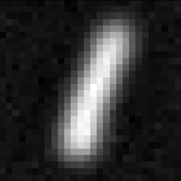
Figure 1: Observation (Left) and reconstruction (Right)

Figure 1 shows an example observation and ground-truth pair. For the purpose of recovering an approximation to $x_{\text{true}}$ using our observation $y$, we formulate a minimisation problem given by

$$\min_{x}\left\{f(x):=\frac{1}{2}\|Ax-y\|_{2}^{2}+\alpha H_{\epsilon}(x)\right\},$$ (7.0.1)

with $\alpha=10^{-4}$, and $H_{\epsilon}$ given as the Huber regularised Total Variation [13, 19] with $\epsilon=0.01$, defined as

$$H_{\varepsilon}(\mathrm{D}u)=\sum_{i=1,j=1}^{m,n}h_{\varepsilon}\left(\sqrt{(\mathrm{D}u)_{i,j,1}^{2}+(\mathrm{D}u)_{i,j,2}^{2}}\right),$$ (7.0.2)

with the Huber loss defined as

$$h_{\varepsilon}(s)=\begin{cases}\frac{1}{2\varepsilon}{s^{2}},\text{ if }|s|\leq\varepsilon\\ |s|-\frac{\varepsilon}{2},\text{ otherwise},\end{cases}$$ (7.0.3)

and the gradient operator $\mathrm{D}:\mathbb{R}^{m\times n}\rightarrow\mathbb{R}^{m\times n\times 2}$ equal to

$$(\mathrm{D}u)_{i,j,1}=\begin{cases}u_{i+1,j}-u_{i,j}&\text{ if }1\leq i<m,\\ 0&\text{ else },\end{cases}$$ (7.0.4)

$$(\mathrm{D}u)_{i,j,2}=\begin{cases}u_{i,j+1}-u_{i,j}&\text{ if }1\leq j<n,\\ 0&\text{ else. }\end{cases}$$ (7.0.5)

Then, each function $f$ is $L$-smooth, where [5]

$$L=\|A\|^{2}+\frac{\alpha\|D\|^{2}}{\varepsilon}\leq 1+\frac{8\alpha}{\varepsilon}=1.08.$$ (7.0.6)

Learning preconditioners $G_{\theta_{t}}$:

Let

$$\mathcal{X}_{k}=\{x\in\mathcal{X}:x\text{ has label }k\},$$ (7.0.7)

then define the training set and two testing sets by the following:

• Training set: Image set $\mathcal{T}_{1,1}\subset\mathcal{X}_{1}$ of MNIST ones, with $|\mathcal{T}_{1,1}|=1000$ .

• Testing set $1$: Image set $\mathcal{T}_{1,2}\subset\mathcal{X}_{1,2}$ of MNIST ones not in training set, with $|\mathcal{T}_{1,2}|=100$.

• Testing set $2$: Image set $\mathcal{T}_{2}\subset\mathcal{X}\setminus\mathcal{X}_{1}$ of MNIST digits in $\{2,3,4,5,6,7,8,9,0\}$, with $|\mathcal{T}_{2}|=100$.

The learned convolutional kernel is chosen to be of size $28\times 28$.

At iteration $t$, for a parametrisation $G_{\theta}$, we learn $\theta_{t}$ via the following procedure, for a tolerance $\nu=10^{-3}$ we have the stopping condition given by

$$\frac{\|\nabla g_{t}(\theta_{t}^{w})\|_{2}}{\|\nabla g_{t}(\tilde{\theta})\|_{2}}<\nu,$$ (7.0.8)

at some sub-iteration $w$, for $\tilde{\theta}$ defined in (6.0.19) and $\theta_{t}^{w}$ as in (5.0.1). A stopping iteration $\tilde{T}=5000$ is also used, such that if the optimisation algorithm hasn’t terminated due to the criterion (7.0.8), set $\theta_{t}=\theta_{t}^{\tilde{T}}$.

Preconditioners are learned up to iteration $T=100$, such that we learn preconditioners $G_{\theta_{0}},\cdots,G_{\theta_{99}}$, for our parameterisations (P1-P4) in Table 1.

Comparison of learned parametrisations with classical hand-crafted optimisation algorithms

In Figure 2, we see the performance of the learned preconditioners over the first $100$ iterations against gradient descent with a constant step size equal to $1/L$. In particular, we see that, despite the diagonal preconditioner and the convolutional preconditioner having the same number of parameters, the convolutional preconditioner dramatically outperforms the diagonal preconditioner in this numerical experiment. In this case, there is evidence that adding local information is more important than adding pixel-specific flexibility.

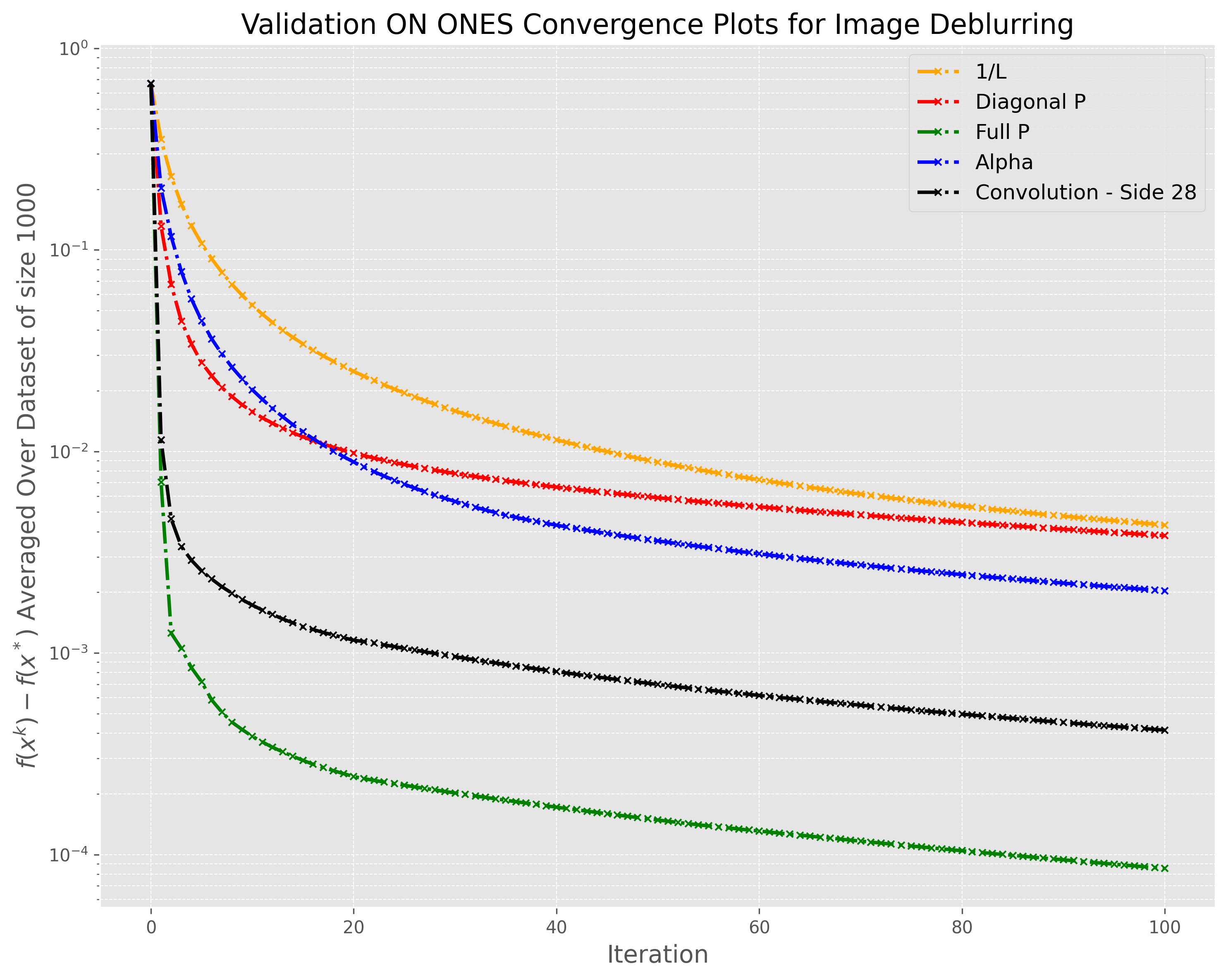
Figure 2: Performance of learned preconditioners on the test set $\mathcal{T}_{1,2}$, compared to a step-size given by $1/L$. On the $x$-axis, we have the iteration number, and on the $y$-axis, we have $f_{k}(x_{k}^{t})-f_{k}^{*}$ averaged over all data points.

Furthermore, we see more comparisons in Figure 3. For example, in the left image, we compare our learned preconditioning with FISTA and BFGS. The methods we learned initially significantly outperformed these methods. However, these handcrafted methods outperform at further iterations, as shown in Figure 4. Figure 5 shows that these further iterations may be of little importance as the images at these iterations are very similar to those at slightly higher objective values.

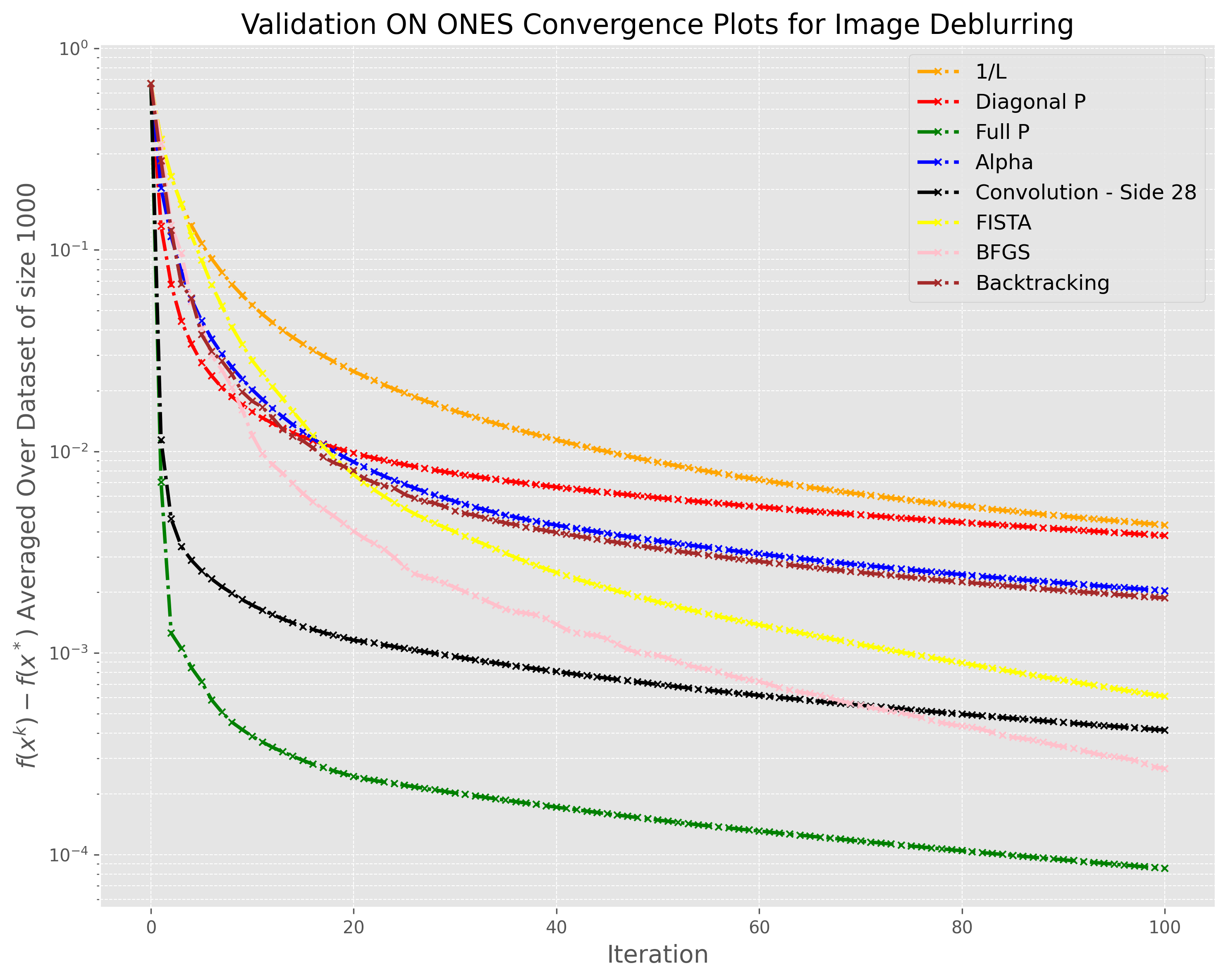
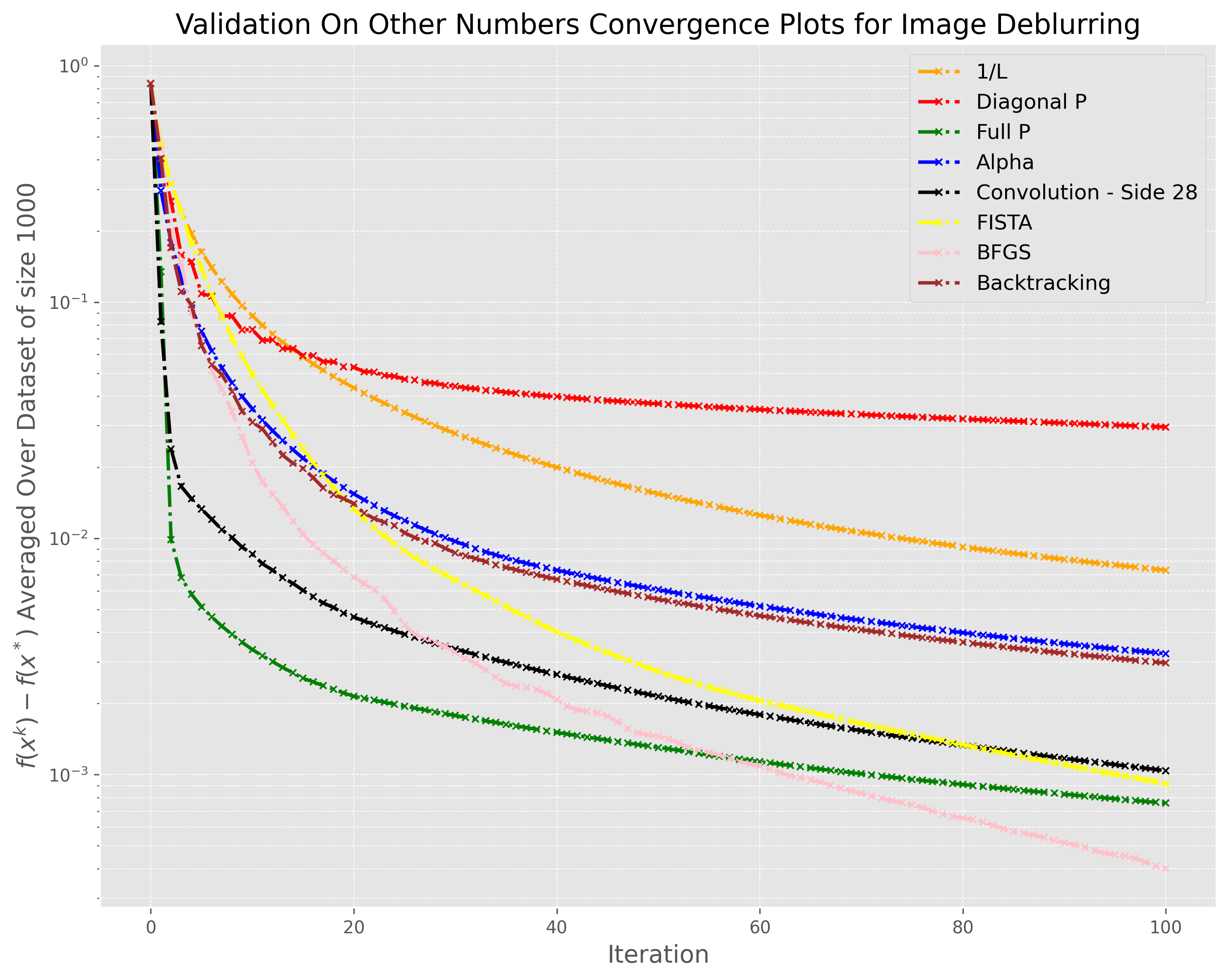
Figure 3: (Left) Performance of learned preconditioners on the test set $\mathcal{T}_{1,2}$, compared to a step-size given by $1/L$, backtracking line-search, and BFGS. (Right) Performance of learned preconditioners on the test set $\mathcal{T}_{2}$, compared to a step-size given by $1/L$, backtracking line-search, and BFGS.

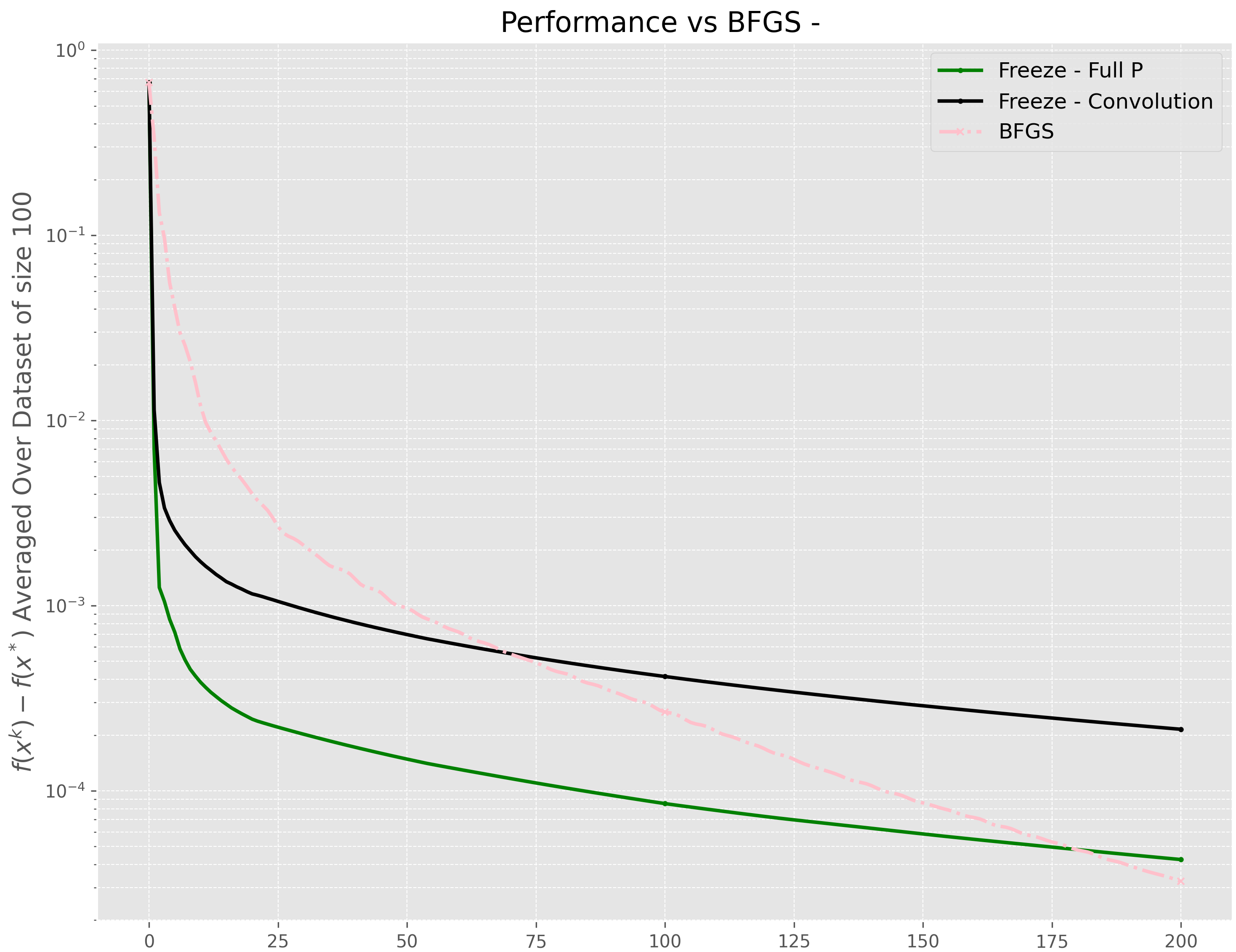
Figure 4: A comparison of the learned convolutional and full matrix preconditioners to BFGS on the test set $\mathcal{T}_{1,2}$. We observe much faster initial convergence for the learned methods, but BFGS is eventually overtaken. In Figure 5, we see this may not be relevant as the images do not visually change much below a loss of $\frac{5}{10^{4}}$.

Iteration 10

Iteration 20

Iteration 50

Iteration 90

Full

Convolution

BFGS

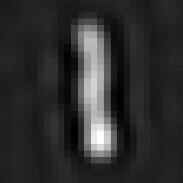
Figure 5: A comparison of BFGS, convolution and full matrix preconditioning reconstructions.

Freeze vs recycle

Now we compare whether freezing our final preconditioner or recycling all learned preconditioners is favourable. Figure 6 shows that recycling preconditioners can produce more unstable behaviour, for example, in the case of the learned step-sizes in blue and the learned full matrix in green. In the case of the learned full matrix, however, we see that the final performance is better when recycling preconditioners. However, when freezing the final preconditioner, the learned diagonal preconditioner leads to divergence. Therefore, it is not obvious which choice is better; it depends on which parameterisation is under consideration.

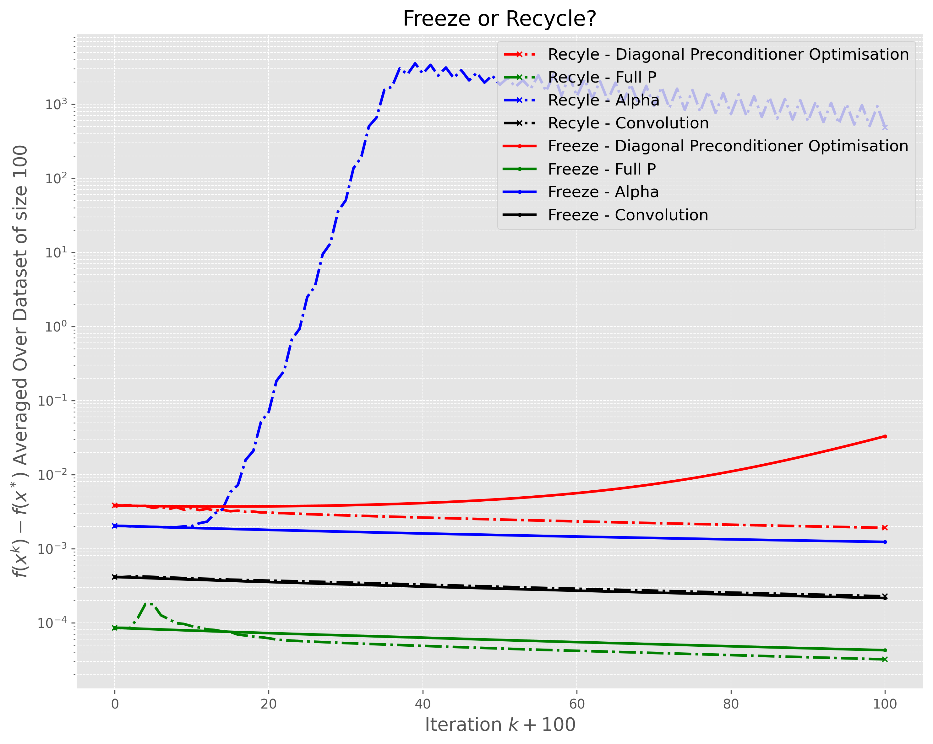
Figure 6: Performance comparison freezing the final preconditioner vs recycling the final preconditioner on iterations AFTER training, i.e. starting at iteration $100$.

Learned preconditioners:

Now, we visualise the learned parameters for convolutional and diagonal preconditioning and learned step sizes. We see learned convolutional kernels in Figures 8 and 9. Note that these learned kernels contain negative values. While this does not necessarily imply that the corresponding matrices learned are not positive-definite, in Figures 11 and 12, we see that the learned diagonals have negative values, meaning that the learned matrices are not positive-definite!

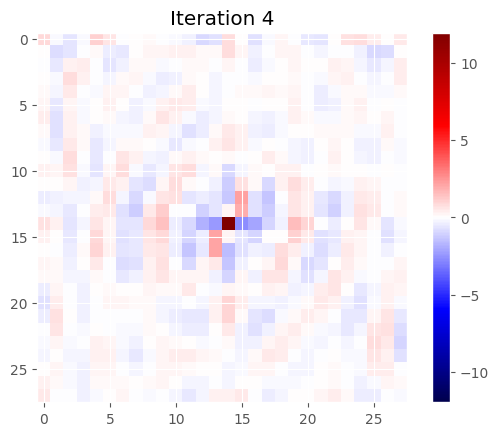
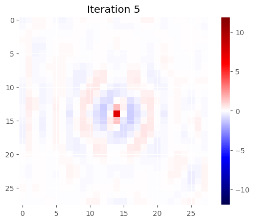
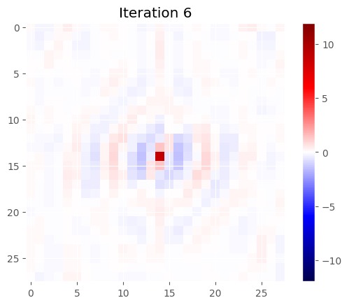
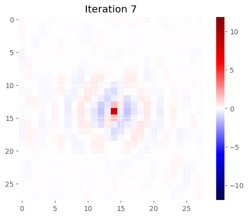
Figure 8: Learned convolutional kernels for the first $8$ images, on the same scale.

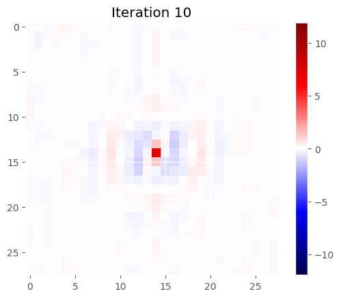
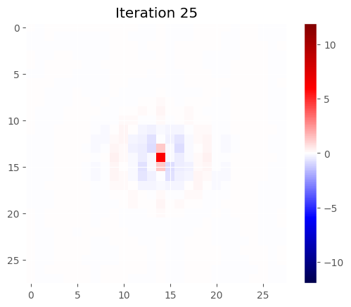
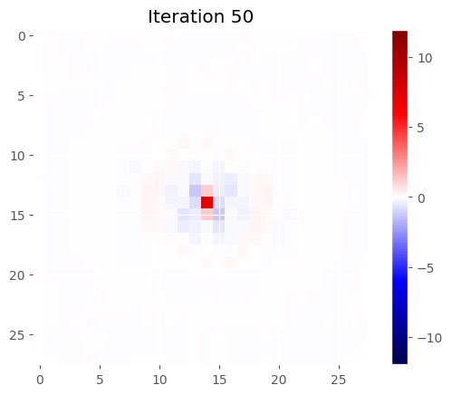
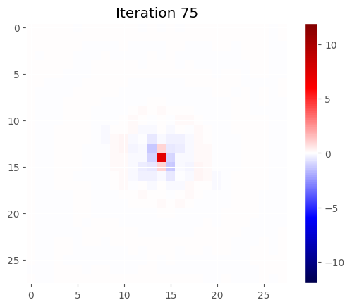
Figure 9: Learned convolutional kernels at iteration $10,25,50,75$.

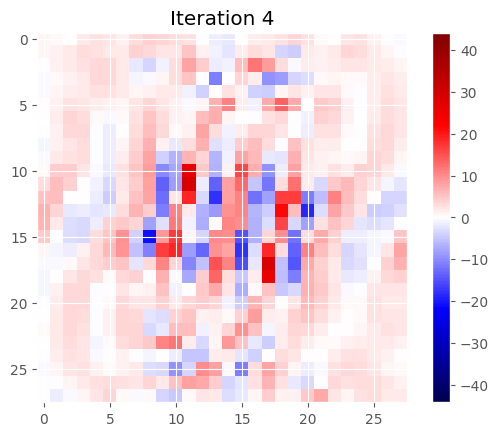
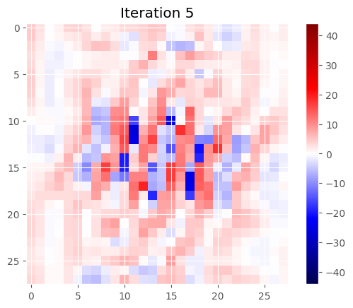
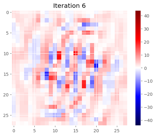
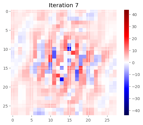
Figure 11: Learned diagonal preconditioner (reshaped to an image) for the first $8$ images, on the same scale.

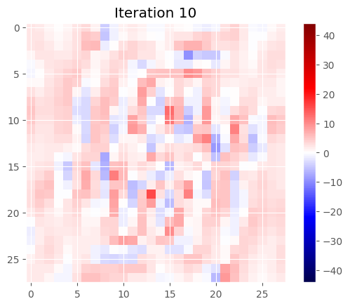
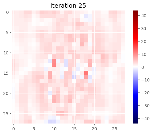
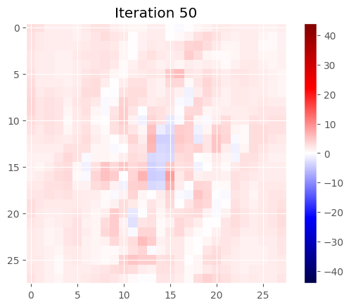
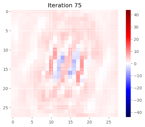
Figure 12: Learned diagonal preconditioner (reshaped to an image) at iteration $10,25,50,75$.

Figure 13 shows learned step sizes. Note that these values often fluctuate up and down. Furthermore, the learned step sizes are initially all greater than $2/L$ and, therefore, out of the range of provable convergence. However, after iteration $55$, the learned step sizes fluctuate above and below this threshold.

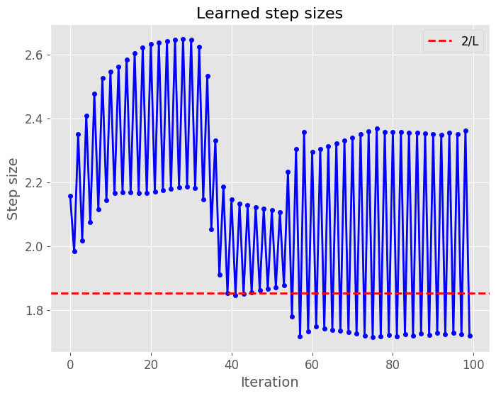
Figure 13: Learned step sizes.

8 Conclusions and future work

8.1 Conclusions

This paper introduced how one can learn preconditioners for gradient descent for use in ill-conditioned optimisation problems. We formulated how to generate a sequence of preconditioners learned using a convex optimisation problem on a dataset such that

• The preconditioners need not be positive definite, nor symmetric,

• the preconditioner at iteration $t$ is constant over all functions,

• these preconditioners have a closed-form equation for least-squares problems,

• and convergence is guaranteed for all functions in the training set,

• with proved convergence rates for each train function.

• Empirical performance was tested, with good results, especially for convolutional preconditioning in the image deblurring example, with maintained performance on out-of-distribution test images.

8.2 Future Work

As was seen in the numerical experiments, despite the tremendous early-iteration performance of the full-matrix and convolutional preconditioning, we saw that the performance of FISTA eventually overtook that of the learned algorithms. Future research aims to extend these learned methods to include momentum terms. One way of achieving this is to extend the minimisation problem (3.0.5) to include a momentum preconditioner.

One potential drawback of the learned preconditioning is not knowing $\lim_{t\to\infty}G_{\theta_{t}}$, which limits the convergence analysis on unseen data. To remedy this, one can introduce regularisation of the learned parameters. Another use of regularisation is to encourage preconditioners to exhibit specific behaviours. One may encourage preconditioners to exhibit symmetry or smoothness, for example.

This paper considered only diagonal, full matrices, and convolution, which is not an exhaustive list of potential parametrisations. Despite significantly fewer parameters learned, we saw that convolution may offer a more expressive update than the diagonal preconditioner. One could also consider an update similar to Quasi-Newton methods.

This paper only considered an explicit dataset of functions $f_{1},\cdots,f_{N}$, equivalent to sampling from the class of functions $\mathcal{F}$ using a Dirac delta distribution. One can instead consider sampling from a class of function $\mathcal{F}$ using an arbitrary probability distribution.

Finally, in this paper, we only considered learning a matrix preconditioner. Future work would extend this to consider preconditioners as a function of $x_{t}$ and $\nabla f(x_{t})$, for example.

Appendix A Nonconvexity for multiple steps

This can be seen as

$$f(x_{2}(\theta_{0},\theta_{1})) =f(x_{1}-G_{\theta_{1}}(\nabla f(x_{1}(\theta_{0})))$$ (A.0.1)

$$=f(x_{0}-G_{\theta_{0}}(\nabla f(x_{0}))-G_{\theta_{1}}(\nabla f(x_{0}-G_{\theta_{0}}(\nabla f(x_{0}))))$$ (A.0.2)

is non-convex in general. In particular, if we wish to learn a single step-size $\alpha$ for a least-squares function $f(x)=\frac{1}{2}\|Ax-y\|$, then $\nabla f(x)=A^{T}(Ax-y)$ and

$$f(x_{2}(\alpha)) =f(x_{0}-\alpha\nabla f(x_{0})-\alpha A^{T}(A(x_{0}-\alpha\nabla f(x_{0}))-y)$$ (A.0.4)

$$=f(x_{0}-\alpha\nabla f(x_{0})-\alpha A^{T}Ax_{0}+\alpha^{2}A^{T}A\nabla f(x_{0})-\alpha A^{T}y)$$ (A.0.5)

and we see we get the composition of a quadratic function in $\alpha$ with $f$, which is not convex in general. If we consider $h(x)$ convex and define $q(x)=h(x_{2})$, then assuming that $q$ is convex, we have

$$q(0)=q\left(\frac{1}{2}x+\frac{1}{2}(-x)\right)\leq\frac{1}{2}q(x)+\frac{1}{2}q(-x)=h(x_{2}),$$ (A.0.7)

a contradiction.

References

• [1] Marcin Andrychowicz, Misha Denil, Sergio Gomez, Matthew W Hoffman, David Pfau, Tom Schaul, Brendan Shillingford, and Nando De Freitas. Learning to learn by gradient descent by gradient descent. Advances in neural information processing systems, 29, 2016.
• [2] Sebastian Banert, Axel Ringh, Jonas Adler, Johan Karlsson, and Ozan Oktem. Data-driven nonsmooth optimization. SIAM Journal on Optimization, 30(1):102–131, 2020.
• [3] Amir Beck. Introduction to nonlinear optimization: Theory, algorithms, and applications with MATLAB. SIAM, 2014.
• [4] Silvia Bonettini, Ignace Loris, Federica Porta, and Marco Prato. Variable metric inexact line-search-based methods for nonsmooth optimization. SIAM journal on optimization, 26(2):891–921, 2016.
• [5] Antonin Chambolle and Thomas Pock. An introduction to continuous optimization for imaging. Acta Numerica, 25:161–319, 2016.
• [6] Tianlong Chen, Xiaohan Chen, Wuyang Chen, Howard Heaton, Jialin Liu, Zhangyang Wang, and Wotao Yin. Learning to optimize: A primer and a benchmark. Journal of Machine Learning Research, 23(189):1–59, 2022.
• [7] William C Davidon. Variable metric method for minimization. SIAM Journal on optimization, 1(1):1–17, 1991.
• [8] Li Deng. The mnist database of handwritten digit images for machine learning research [best of the web]. IEEE signal processing magazine, 29(6):141–142, 2012.
• [9] Matthias J Ehrhardt, Pawel Markiewicz, and Carola-Bibiane Schönlieb. Faster pet reconstruction with non-smooth priors by randomization and preconditioning. Physics in Medicine & Biology, 64(22):225019, 2019.
• [10] Roger Fletcher. A new approach to variable metric algorithms. The computer journal, 13(3):317–322, 1970.
• [11] Paul Häusner, Ozan Öktem, and Jens Sjölund. Neural incomplete factorization: learning preconditioners for the conjugate gradient method. arXiv preprint arXiv:2305.16368, 2023.
• [12] Tao Hong, Xiaojian Xu, Jason Hu, and Jeffrey A Fessler. Provable preconditioned plug-and-play approach for compressed sensing mri reconstruction. arXiv preprint arXiv:2405.03854, 2024.
• [13] Peter J Huber. Robust estimation of a location parameter. In Breakthroughs in statistics: Methodology and distribution, pages 492–518. Springer, 1992.
• [14] Kirsten Koolstra and Rob Remis. Learning a preconditioner to accelerate compressed sensing reconstructions in mri. Magnetic Resonance in Medicine, 87(4):2063–2073, 2022.
• [15] Ke Li and Jitendra Malik. Learning to optimize. arXiv preprint arXiv:1606.01885, 2016.
• [16] Vishal Monga, Yuelong Li, and Yonina C Eldar. Algorithm unrolling: Interpretable, efficient deep learning for signal and image processing. IEEE Signal Processing Magazine, 38(2):18–44, 2021.
• [17] Yurii Nesterov et al. Lectures on convex optimization, volume 137. Springer, 2018.
• [18] Jorge Nocedal and Stephen J Wright. Numerical optimization. Springer, 1999.
• [19] Leonid I Rudin, Stanley Osher, and Emad Fatemi. Nonlinear total variation based noise removal algorithms. Physica D: nonlinear phenomena, 60(1-4):259–268, 1992.
• [20] Hong Ye Tan, Subhadip Mukherjee, Junqi Tang, and Carola-Bibiane Schönlieb. Data-driven mirror descent with input-convex neural networks. SIAM Journal on Mathematics of Data Science, 5(2):558–587, 2023.
• [21] Singanallur V Venkatakrishnan, Charles A Bouman, and Brendt Wohlberg. Plug-and-play priors for model based reconstruction. In 2013 IEEE global conference on signal and information processing, pages 945–948. IEEE, 2013.