Model-based Clustering of Zero-Inflated Single-Cell RNA Sequencing Data via the EM Algorithm

Abstract

Biological cells can be distinguished by their phenotype or at the molecular level, based on their genome, epigenome, and transcriptome. This paper focuses on the transcriptome, which encompasses all the RNA transcripts in a given cell population, indicating the genes being expressed at a given time. We consider single-cell RNA sequencing data and develop a novel model-based clustering method to group cells based on their transcriptome profiles. Our clustering approach takes into account the presence of zero inflation in the data, which can occur due to genuine biological zeros or technological noise. The proposed model for clustering involves a mixture of zero-inflated Poisson or zero-inflated negative binomial distributions, and parameter estimation is carried out using the EM algorithm. We evaluate the performance of our proposed methodology through simulation studies and analyses of publicly available datasets.

1 Introduction

For many years, researchers have been interested in discovering more about the distinct cell types in multi-cellular organisms. For this purpose, researchers can differentiate cells by phenotype, such as size and shape or at the molecular level, based on their genome, epigenome, and transcriptome. In this paper, we focus on the transcriptome, which includes all ribonucleic acid (RNA) transcripts present in a given cell population, indicating the genes being expressed at any given time. Transcriptome analyses can be conducted at the bulk level, where the transcriptome of thousands or millions of cells is measured and averaged simultaneously (Mortazavi et al., 2008; Cloonan et al., 2008). Alternatively, gene expression profiling can be carried out at the single-cell level, offering a powerful, high-resolution tool for biological and medical discoveries (Saliba et al., 2014; Trapnell, 2015; Tanay and Regev, 2017; Qu et al., 2023; Jovic et al., 2021; Heumos et al., 2023). Therefore, the development of statistical and computational methods to analyze single-cell RNA sequencing (scRNA-seq) data is critical for researchers to assess the heterogeneity between individual cells and identify cell types based on their transcriptome (Macaulay and Voet, 2014; Andrews and Hemberg, 2018).

The process of scRNA-seq includes the following main steps: creating single-cell suspension using an isolation method; cell lysis (with or without whole genome amplification); library preparation and sequencing; and, finally, mapping the reads to the reference genome. Thus, the expression of a gene can be measured by the number of reads aligned within its genomic coordinates (the so-called read counts or counts). Therefore, scRNA-seq data arise as a count matrix with counts across genes over each cell upon sequencing. Because the amount of RNA material per cell is limited, some transcripts are not detected during sequencing, leading to high dropouts (zero counts) in the generated scRNA-seq data (Kharchenko et al., 2014). In addition, some of the observed zero counts may correspond to true biological zeros (no expression). This leads to an excess of zeros (zero-inflation) in the count matrix of scRNA-seq data, an important characteristic of these data. This feature of zero-inflation poses some challenges for the statistical analysis of scRNA-seq data, where most methods for bulk RNA-seq data should be modified for scRNA-seq data or novel methods should be developed (Lähnemann et al., 2020).

Analysis of scRNA-seq data requires statistical methods for various undertakings including, but not limited to, quality control, normalization of raw read counts, feature extraction, dimensionality reduction, cell clustering and identification of differentially expressed genes (O. Stegle and Marioni, 2015; Heumos et al., 2023). In this paper, we focus on cell clustering. Therefore, we aim to develop a model-based clustering approach for cell type identification capable of dealing with the zero-inflated count data.

Different model-based clustering methods have been developed to analyze scRNA-seq data. These methods include TSCAN (Ji and Ji, 2016), BISCUIT (Prabhakaran et al., 2016), DIMM-SC (Sun et al., 2018), BasClu (Liu et al., 2019), and CellAssign (Zhang et al., 2019). After dimensionality reduction via PCA, TSCAN employs a mixture of multivariate Gaussian distributions to cluster cells based on their gene expression. BISCUIT uses a hierarchical Bayesian Dirichlet process mixture model, assuming gene log counts follow a Gaussian distribution. BasClu extends the Dirichlet process mixture model of BISCUIT to account for zero counts and dropout events by introducing a sequence of latent binary indicators and modelling the probability of missing data across genes. DIMM-SC proposes a Dirichlet mixture model for clustering droplet-based scRNA-seq data, assuming gene read counts follow a multinomial distribution. Lastly, CellAssign considers a mixture of negative binomial distributions and prior knowledge of some cell-type marker genes to classify cells.

So far, most available clustering tools for scRNA-seq data do not tackle the issue of zero inflation, especially non-model-based tools such as distance-based methods (Kiselev et al., 2017; Wang et al., 2017; Grun et al., 2016; Kim et al., 2018; Žurauskienė and Yau, 2016; Zeisel et al., 2015) or graph-based approaches (Wei et al., 2022; Liu, 2021; Wolf et al., 2018; Shi and Huang, 2017; Satija et al., 2015; Levine et al., 2015; Xu and Su, 2015). In some studies, zero inflation is tackled in the dimensionality reduction or feature selection step of the analysis, which is usually carried out prior to clustering. For example, Pierson and Yau (2015) developed a dimensionality reduction technique, ZIFA, which considers the zero inflation of scRNA-seq data, and they demonstrated that in comparison with other dimensionality reduction methods, ZIFA performs better in both simulated and biological data sets. Also, Tian et al. (2019, 2021) consider a zero-inflated negative binomial model-based loss function autoencoder for dimensionality reduction followed by a deep-embedded clustering algorithm. Qiu (2020) tackles the zero-inflation problem by first binarizing the scRNA-seq data, turning all the non-zero observations into one, and then proposing a non-probabilistic multi-step clustering method to cluster the binarized data.

In this paper, we aim to cluster cells based on their scRNA-seq data using a model-based approach that directly considers the zero-inflated distribution of the raw counts (number of reads aligned to each gene), thus addressing a significant gap in previous studies. We assume a probabilistic model in which scRNA-seq data follows a mixture of either zero-inflated Poisson (ZIP) or zero-inflated negative binomial (ZINB) distributions. We also allow the logarithm of the rate parameter of the Poisson or negative binomial component to be a linear combination of some fixed and known covariates, such as batch effects and cell size factor. We estimate cluster assignments and model parameters via the Expectation-Maximization (EM) algorithm (Dempster et al., 1977; McLachlan and Krishnan, 2008). We implement our proposed methodology using R, and the code is available online at https://github.com/desouzalab/em-mzip.

This paper is organized as follows. In Section 2, our novel model-based methodology for clustering zero-inflated counts is presented. Simulation results under various scenarios are presented in Section 3. Real data applications of the proposed models are studied in Section 4. Finally, the conclusion and final remarks are discussed in Section 5.

2 Method

Our model-based clustering approach assumes that the scRNA-seq count data arise from a mixture of zero-inflated Poisson (ZIP) or zero-inflated negative binomial (ZINB) distributions. Section 2.1 presents the proposed mixture model and EM algorithm for zero-inflated Poisson counts, considering the cases without and with covariates. In Section 2.2, we describe our proposed methodology for the mixture of ZINB distributions, also covering cases without and with covariates.

2.1 The proposed mixture model for ZIP counts

Let $Y_{ng}$ be a random variable for the number of read counts aligned to gene $g$ in cell $n$, for $g=1,\dots,G$ and $n=1,\dots,N$, where $Y_{ng}$ takes a value in $\{0,1,2,3,\dots\}$. So, the observed data can be written in the following matrix format:

$$\mathbf{y}=\begin{pmatrix}y_{11}&y_{12}&\cdots&y_{1G}\\ y_{21}&y_{22}&\cdots&y_{2G}\\ \vdots&\vdots&\ddots&\vdots\\ y_{N1}&y_{N2}&\cdots&y_{NG}\end{pmatrix}.$$ (1)

Suppose that there are $K\ll N$ clusters of cells and let $\boldsymbol{Z}=\{Z_{11},\dots,Z_{NK}\}$ be the set of latent random variables indicating the true cell cluster assignments, that is:

$$Z_{nk}=\begin{dcases*}1,&if cell $n$ belongs to cluster $k$,\\ 0,&otherwise.\end{dcases*}$$ (2)

with $\sum_{k=1}^{K}Z_{nk}=1$, $P(Z_{nk}=1)=\pi_{k}$ for $n=1,\dots,N$, $k=1,\dots,K$, and $\sum_{k=1}^{K}\pi_{k}=1$. We assume that given $Z_{nk}=1$, $Y_{n1},\ldots,Y_{nG}$ are independent and follow a ZIP distribution with parameters that depend on cluster $k$. Let $\boldsymbol{\theta}=\{\boldsymbol{\theta}_{1},\dots,\boldsymbol{\theta}_{K}\}$ be the set of all models parameters with $\boldsymbol{\theta}_{k}=\{\pi_{k},\phi_{k},\boldsymbol{\lambda}_{k}\}$, and $\boldsymbol{\lambda_{k}}=\{\lambda_{1k},\dots,\lambda_{Gk}\}$. Thus, we can write the probability mass function (pmf) for each cell as the following mixture of zero-inflated Poisson (ZIP) distributions:

$$p(\mathbf{y}_{n}\,|\,\boldsymbol{\theta})=\sum_{k=1}^{K}\pi_{k}p(\mathbf{y}_{n}\,|\,\boldsymbol{\theta}_{k})=\sum_{k=1}^{K}\pi_{k}\prod_{g=1}^{G}p(y_{ng}\,|\,\lambda_{gk},\phi_{k}),$$

where

$$p(y_{ng}\,|\,\lambda_{gk},\phi_{k})=\begin{dcases*}\phi_{k}+(1-\phi_{k})e^{-\lambda_{gk}},&if $y_{ng}=0$,\\ (1-\phi_{k})\frac{e^{-\lambda_{gk}}\lambda_{gk}^{y_{ng}}}{y_{ng}!},&if $y_{ng}=1,2,3,\dots$,\end{dcases*}$$ (3)

in which $\lambda_{gk}$ is the Poisson rate parameter and $\phi_{k}$ is the probability of always (or perfect) zero. By assuming independence across cells, the observed-data log-likelihood based on all cells is given by:

$$\ell(\boldsymbol{\theta}\,|\,\boldsymbol{y})=\sum_{n=1}^{N}\log\left[\sum_{k=1}^{K}\pi_{k}\prod_{g=1}^{G}p(y_{ng}\,|\,\lambda_{gk},\phi_{k})\right].$$ (4)

The goal is to find the parameter estimates that maximize $\ell(\boldsymbol{\theta}\,|\,\boldsymbol{y})$ in (4), but we cannot do it analytically with a closed formula. To tackle this problem, we develop an EM algorithm to iteratively find the parameter estimates. To obtain these estimates using the EM framework, we consider the true latent cluster assignments $Z_{nk}$ for $n=1,\dots,N$ and $k=1,\dots,K$ as in (2). In addition, we introduce another set of hidden variables $\boldsymbol{U}=\{U_{11},\ldots,U_{NG}\}$, where each $U_{ng}$, for $n=1,\ldots,N$ and $g=1,\ldots,G$, is defined as follows:

$$U_{ng}=\begin{dcases*}1,&if $y_{ng}$ is from the perfect zero state,\\ 0,&if $y_{ng}$ is from the Poisson state.\end{dcases*}$$

This latent indicator variable is drawn from a Bernoulli distribution that depends on the cluster $k$, $U_{ng}\mid Z_{nk}=1\sim$ Bernoulli($\phi_{k}$), with probability of success (for this case, probability of always zero) $\phi_{k}$, defined as $\phi_{k}=P(U_{ng}=1|Z_{nk}=1)$.

In the E-step of the EM algorithm to maximize the observed-data log-likelihood, first we obtain the conditional expectation of the complete-data log-likelihood, and maximize it given the observed data and current parameter estimates is obtained. Then, in the M-step, the expectation from the E-step is maximized with respect to each parameter of interest. These two steps are executed iteratively until convergence. Now, considering the observed counts and the introduced latent variables, the complete-data log-likelihood can be written as:

$$\ell(\boldsymbol{\theta}\,|\,\boldsymbol{y},\boldsymbol{u},\boldsymbol{z})= \sum_{n=1}^{N}\sum_{k=1}^{K}z_{nk}\log\pi_{k}+\sum_{n=1}^{N}\sum_{k=1}^{K}\sum_{g=1}^{G}\Big{(}z_{nk}u_{ng}\log\phi_{k}+z_{nk}(1-u_{ng})\log(1-\phi_{k})\Big{)}$$

$$+\sum_{n=1}^{N}\sum_{k=1}^{K}\sum_{g=1}^{G}z_{nk}(1-u_{ng})\log\left(\frac{e^{-\lambda_{gk}}\lambda_{gk}^{y_{ng}}}{y_{ng}!}\right).$$

In what follows, we present the E and M steps of our proposed EM algorithm for the case without covariates (Section 2.1.1) and the case with covariates (Section 2.1.2).

2.1.1 EM for the ZIP mixture model without covariates

E-Step: We first write the conditional expectation of the complete-data log-likelihood given the current estimates of the parameters, $\boldsymbol{\theta}^{(t)}=\{\boldsymbol{\lambda}^{(t)},\,\boldsymbol{\phi}^{(t)},\,\boldsymbol{\pi}^{(t)}\}$, and the observed data, $\boldsymbol{y}$:

$$Q(\boldsymbol{\theta};\boldsymbol{\theta}^{(t)})= E\Big{[}\ell(\boldsymbol{\theta}\,|\,\boldsymbol{y},\boldsymbol{u},\boldsymbol{z})\,|\,\boldsymbol{y},\boldsymbol{\theta}^{(t)}\Big{]}$$

$$= \sum_{n=1}^{N}\sum_{k=1}^{K}E\Big{[}Z_{nk}\,|\,\boldsymbol{y},\boldsymbol{\theta}^{(t)}\Big{]}\log\pi_{k}$$

$$+\sum_{n=1}^{N}\sum_{k=1}^{K}\sum_{g=1}^{G}\Bigg{(}E\Big{[}Z_{nk}U_{ng}\,|\,\boldsymbol{y},\boldsymbol{\theta}^{(t)}\Big{]}\log\phi_{k}+E\Big{[}Z_{nk}(1-U_{ng})\,|\,\boldsymbol{y},\boldsymbol{\theta}^{(t)}\Big{]}\log(1-\phi_{k})\Bigg{)}$$

$$+\sum_{n=1}^{N}\sum_{k=1}^{K}\sum_{g=1}^{G}E\Big{[}Z_{nk}(1-U_{ng})\,|\,\boldsymbol{y},\boldsymbol{\theta}^{(t)}\Big{]}\log\Bigg{(}\frac{e^{-\lambda_{gk}}\lambda_{gk}^{y_{ng}}}{y_{ng!}}\Bigg{)}$$ (5)

Then, we can show that the expectations in (2.1.1) are as follows:

$$\hat{Z}_{nk}^{(t)} =E\Big{[}Z_{nk}\,|\,\boldsymbol{y}\,,\,\boldsymbol{\theta}^{(t)}\Big{]}$$

$$=E\Big{[}Z_{nk}\,|\,\boldsymbol{y}_{n}\,,\,\boldsymbol{\theta}^{(t)}\Big{]}$$

$$=p\Big{(}Z_{nk}=1\,|\,\boldsymbol{y}_{n}\,,\,\boldsymbol{\theta}^{(t)}\Big{)}$$

$$=\frac{\pi_{k}^{(t)}\prod_{g=1}^{G}p\Big{(}y_{ng}\,|\,\lambda_{kg}^{(t)},\phi_{k}^{(t)}\Big{)}}{\sum_{j=1}^{K}\pi_{j}^{(t)}\prod_{g=1}^{G}p\Big{(}y_{ng}\,|\,\lambda_{jg}^{(t)},\phi_{j}^{(t)}\Big{)}}\mbox{,}$$ (6)

and

$$E\big{[}Z_{nk}U_{ng}\,\big{|}\,\boldsymbol{y},\boldsymbol{\theta}^{(t)}\big{]} =p(Z_{nk}=1,U_{ng}=1\,\big{|}\,\boldsymbol{y},\boldsymbol{\theta}^{(t)})$$

$$=p(U_{ng}=1\,\big{|}\,Z_{nk}=1,y_{ng},\boldsymbol{\theta}^{(t)})\,\times\,p(Z_{nk}=1\,\big{|}\,\boldsymbol{y}_{n},\boldsymbol{\theta}^{(t)})=\hat{U}_{ngk}^{(t)}\hat{Z}_{nk}^{(t)},$$

where $\hat{Z}_{nk}^{(t)}$ is as in (2.1.1) and $\hat{U}_{ngk}^{(t)}=p(U_{ng}=1\,\big{|}\,Z_{nk}=1,y_{ng},\boldsymbol{\theta}^{(t)})$ is given by:

$$\hat{U}_{ngk}^{(t)}=\begin{dcases*}\frac{\phi_{k}^{(t)}}{\Big{(}\phi_{k}^{(t)}+(1-\phi_{k}^{(t)})e^{-\lambda_{gk}^{(t)}}\Big{)}},&if $y_{ng}=0$,\\ 0,&if $y_{ng}=1,2,\dotsc\ $.\end{dcases*}$$ (7)

Note that $\hat{U}_{ngk}^{(t)}$ in (7) is separated into two cases because if $U_{ng}=1$, $y_{ng}$ can only be equal to zero, otherwise, if $y_{ng}$ takes a non-zero count value, it definitely arises from the Poisson state.

Using the calculated values $\hat{Z}_{nk}^{(t)}$ and $\hat{U}_{ngk}^{(t)}$ from Equations (2.1.1) and (7), we can rewrite $Q(\boldsymbol{\theta};\boldsymbol{\theta}^{(t)})$ in (2.1.1) as:

$$Q(\boldsymbol{\theta};\boldsymbol{\theta}^{(t)}) =Q_{1}(\boldsymbol{\pi};\boldsymbol{\pi}^{(t)})+Q_{2}(\boldsymbol{\phi};\boldsymbol{\phi}^{(t)})+Q_{3}(\boldsymbol{\lambda};\boldsymbol{\lambda}^{(t)}),$$ (8)

where

$$Q_{1}(\boldsymbol{\pi};\boldsymbol{\pi}^{(t)})= \sum_{n=1}^{N}\sum_{k=1}^{K}\hat{Z}_{nk}^{(t)}\log(\pi_{k}),$$ (9)

$$Q_{2}(\boldsymbol{\phi};\boldsymbol{\phi}^{(t)})= \sum_{n=1}^{N}\sum_{k=1}^{K}\sum_{g=1}^{G}\Big{[}\hat{Z}_{nk}^{(t)}\hat{U}_{ngk}^{(t)}\log(\phi_{k})+\hat{Z}_{nk}^{(t)}(1-\hat{U}_{ngk}^{(t)})\log(1-\phi_{k})\Big{]},$$ (10)

and

$$Q_{3}(\boldsymbol{\lambda};\boldsymbol{\lambda}^{(t)})= \sum_{n=1}^{N}\sum_{k=1}^{K}\sum_{g=1}^{G}\Big{\{}\hat{Z}_{nk}^{(t)}(1-\hat{U}_{ngk}^{(t)})\Big{[}-\lambda_{gk}+y_{ng}\log\lambda_{gk}-\log y_{ng}!\Big{]}\Big{\}}.$$

M-step: In this step, we maximize $Q(\boldsymbol{\theta};\boldsymbol{\theta}^{(t)})$ in (8) with respect to $\boldsymbol{\theta}$, obtaining the following updated parameters:

$$\pi_{k}^{(t+1)}= \frac{\sum_{n=1}^{N}\hat{Z}_{nk}^{(t)}}{N},$$ (11)

$$\phi_{k}^{(t+1)}= \frac{\sum_{n=1}^{N}\sum_{g=1}^{G}\hat{Z}_{nk}^{(t)}\hat{U}_{ngk}^{(t)}}{G\sum_{n=1}^{N}\hat{Z}_{nk}^{(t)}},\text{ and}$$ (12)

$$\lambda_{gk}^{(t+1)}= \frac{\sum_{n=1}^{N}\hat{Z}_{nk}^{(t)}(1-\hat{U}_{ngk}^{(t)})y_{ng}}{\sum_{n=1}^{N}\hat{Z}_{nk}^{(t)}(1-\hat{U}_{ngk}^{(t)})}.$$ (13)

Note that the conditional expected value of each $Z_{nk}$ in Equation (2.1.1), obtained at the last iteration $t^{*}$, is used to infer the cluster assignment of each cell. Thus, we obtain the decision that cell $n$ belongs to cluster $k$ if that cluster is the one with the highest expected value (highest probability); that is:

$$\hat{Z}_{nk}=\begin{dcases*}1,&if $\hat{Z}_{nk}^{(t^{*})}=\underset{j\in\{1,\dots,K\}}{\mbox{max}}{\hat{Z}_{nj}^{(t^{*})}}$,\\ 0,&otherwise.\end{dcases*}$$ (14)

Algorithm 1 in the Appendix summarizes the EM algorithm for the ZIP mixture model without covariates.

2.1.2 EM for the ZIP mixture model with covariates

In this case, we assume that the Poisson rate parameters depend on a linear combination of covariates via a log link function as follows:

$$\log\lambda_{ngk}=\log T_{n}+\rho_{gk}+\beta_{0g}+\sum_{p=1}^{P}\beta_{pg}x_{np},$$ (15)

for $n=1,\dotsc,N$, $g=1,\dotsc,G$, $k=1,\dotsc,K$, and $p=1,\dotsc,P$, where $T_{n}$ is a fixed size factor (also known as a Poisson offset variable) for cell $n$ (e.g., sequencing library size), $\rho_{gk}$ is the fixed effect of cluster $k$ on gene $g$, $\beta_{0g}$ is a baseline expression for gene $g$, $x_{n1},\dotsc,x_{nP}$ are $P$ known covariates for cell $n$ (e.g., batch and treatment effects), and $\beta_{1g},\dotsc,\beta_{Pg}$ their corresponding unknown coefficients on gene $g$.

This model with covariates can also be called a mixture of generalized ZIP regression models. We again use the EM algorithm to find the estimated parameters and inferred cluster assignments. Therefore, considering the complete-data log-likelihood as

$$\ell(\boldsymbol{\theta}\,|\,\boldsymbol{y},\boldsymbol{x},\boldsymbol{z},\boldsymbol{u})=\sum_{n=1}^{N}\sum_{g=1}^{G}\sum_{k=1}^{K}\Big{[} z_{nk}\log\pi_{k}+z_{nk}u_{ng}\log\phi_{k}+z_{nk}(1-u_{ng})\,\log(1-\phi_{k})$$

$$+\;z_{nk}(1-u_{ng})\,\log(p(y_{ng}\mid\rho_{gk},\beta_{0g},\beta_{pg}))\Big{]},$$

where $\boldsymbol{\theta}=(\boldsymbol{\pi},\boldsymbol{\phi},\boldsymbol{\rho},\boldsymbol{\beta}_{0},\boldsymbol{\beta})$, with $\boldsymbol{\pi}=(\pi_{1},\dots,\pi_{k})^{T}$, $\boldsymbol{\phi}=(\phi_{1},\dots,\phi_{k})\,^{T}$, $\boldsymbol{\rho}=(\rho_{11},\dots,\rho_{G1},\dots,\rho_{1K},\dots,\rho_{GK})^{T}$, $\boldsymbol{\beta}_{0}=(\beta_{01},\dots,\beta_{0G})^{T}$ and $\boldsymbol{\beta}=(\beta_{11},\dots,\beta_{P1},\dots,\beta_{1G},\dots,\beta_{PG})^{T}$.

E-Step:

Similarly to Section 2.1.1, first in the E-step, we compute the conditional expectation of the complete-data log-likelihood given the observed data and the current parameter estimates as follows:

$$Q(\boldsymbol{\theta};\boldsymbol{\theta}^{(t)})= E\Big{[}\ell(\boldsymbol{\theta}\,|\,\boldsymbol{y},\,\boldsymbol{x},\,\boldsymbol{z},\,\boldsymbol{u}\,)\,|\,\boldsymbol{y},\,\boldsymbol{x},\,\boldsymbol{\theta}^{(t)}\,\Big{]}$$

$$= \sum_{n=1}^{N}\sum_{k=1}^{K}E\Big{[}Z_{nk}\,|\,\boldsymbol{y},\boldsymbol{x},\boldsymbol{\theta}^{(t)}\Big{]}\log(\pi_{k})$$

$$+\sum_{n=1}^{N}\sum_{g=1}^{G}\sum_{k=1}^{K}\Big{(}E\Big{[}Z_{nk}U_{ng}\,|\,\boldsymbol{y},\boldsymbol{x},\boldsymbol{\theta}^{(t)}\Big{]}\log(\phi_{k})+E\Big{[}Z_{nk}(1-U_{ng})\,|\,\boldsymbol{y},\boldsymbol{x},\boldsymbol{\theta}^{(t)}\Big{]}\log(1-\phi_{k})\Big{)}$$

$$+\sum_{n=1}^{N}\sum_{g=1}^{G}\sum_{k=1}^{K}E\Big{[}Z_{nk}(1-U_{ng})\,|\,\boldsymbol{y},\boldsymbol{x},\boldsymbol{\theta}^{(t)}\Big{]}$$

$$\times\left[-\exp\left\{\log T_{n}+\beta_{0g}+\rho_{gk}+\sum_{p=1}^{P}\,\beta_{pg}x_{np}\right\}+y_{ng}\,\left\{\log T_{n}+\beta_{0g}+\rho_{gk}+\sum_{p=1}^{P}\,\beta_{pg}x_{np}\right\}-\log\,y_{ng}!\right]$$ (16)

Similarly to Equations (2.1.1) and (7) in Section 2.1.1, we calculate $\hat{Z}_{nk}^{(t)}$ and $\hat{U}_{ngk}^{(t)}$ as follows:

$$\hat{Z}_{nk}^{(t)}=E\Big{[}Z_{nk}\,|\,\boldsymbol{y},\boldsymbol{x},\boldsymbol{\theta}^{(t)}\Big{]}=\frac{\pi_{k}^{(t)}\prod_{g=1}^{G}p(y_{ng}\,|\,\phi_{k}^{(t)},\rho_{gk}^{(t)},\beta_{0g}^{(t)},\beta_{pg}^{(t)})}{\sum_{k=1}^{K}\pi_{k}^{(t)}\prod_{g=1}^{G}p(y_{ng}\,|\,\phi_{k}^{(t)},\rho_{gk}^{(t)},\beta_{0g}^{(t)},\beta_{pg}^{(t)})}$$ (17)

$$\hat{U}_{ngk}^{(t)}=p\Big{(}U_{ng}=1|Z_{nk}=1,\boldsymbol{x},y_{ng},\boldsymbol{\theta}^{(t)}\Big{)}=\begin{dcases*}\frac{\phi_{k}^{(t)}}{\Big{(}\phi_{k}^{(t)}+(1-\phi_{k}^{(t)})e^{-\lambda_{ngk}^{(t)}}\Big{)}},&if $y_{ng}=0$,\\ 0,&if $y_{ng}=1,2,\dotsc,$\end{dcases*}$$ (18)

where $\lambda_{ngk}^{(t)}=\exp\Big{\{}\log T_{n}+\rho_{gk}^{(t)}+\beta_{0g}^{(t)}+\sum_{p=1}^{P}\beta_{pg}^{(t)}x_{np}\Big{\}}$.

By using the expected values $\hat{Z}_{nk}^{(t)}$ and $\hat{U}_{ngk}^{(t)}$ from Equations (17) and (18), we can rewrite $Q(\boldsymbol{\theta};\boldsymbol{\theta}^{(t)})$ as follows:

$$Q(\boldsymbol{\theta}\,;\,\boldsymbol{\theta}^{(t)}) =Q_{1}(\boldsymbol{\pi}\,;\,\boldsymbol{\pi}^{(t)})+Q_{2}(\boldsymbol{\phi}\,;\,\boldsymbol{\phi}^{(t)})+Q_{3}\Big{(}(\boldsymbol{\beta}_{0},\,\boldsymbol{\rho},\,\boldsymbol{\beta})\,;\,(\boldsymbol{\beta}_{0}^{(t)},\,\boldsymbol{\rho}^{(t)},\,\boldsymbol{\beta}^{(t)}\,)\Big{)}$$

where the form of $Q_{1}(\boldsymbol{\pi}\,;\,\boldsymbol{\pi}^{(t)})$ and $Q_{2}(\boldsymbol{\phi}\,;\,\boldsymbol{\phi}^{(t)})$ remain as in (9) and (10), respectively, and

$$0Q_{3}\Big{(}(\boldsymbol{\beta}_{0},\,\boldsymbol{\rho},\,\boldsymbol{\beta}\,);\,(\boldsymbol{\beta}_{0}^{(t)},\boldsymbol{\rho}^{(t)},\,\boldsymbol{\beta}^{(t)})\Big{)}=\sum_{n=1}^{N}\sum_{g=1}^{G}\sum_{k=1}^{K}\hat{Z}_{nk}^{(t)}(1-\hat{U}_{ngk}^{(t)})\times$$

$$\left[-\exp\left\{\log(T_{n})+\beta_{0g}+\rho_{gk}+\sum_{p=1}^{P}\,\beta_{pg}x_{np}\right\}+y_{ng}\left\{\log(T_{n})+\beta_{0g}+\rho_{gk}+\sum_{p=1}^{P}\,\beta_{pg}x_{np}\right\}-\log\,y_{ng}!\right]$$ (19)

M-Step: In the M-Step, through differentiating $Q(\boldsymbol{\theta}\,;\,\boldsymbol{\theta}^{(t)})$ with respect to each parameter, we can find the updated estimates. We obtain $\pi_{k}^{(t+1)}$ and $\phi_{k}^{(t+1)}$ in closed form as in (11) and (12), respectively, in Section 2.1.1. Next, we find the updated estimates $\beta_{0g}^{(t+1)}$, $\rho_{gk}^{(t+1)}$, and $\beta_{pg}^{(t+1)}$ as the values that maximize $Q_{3}$ in (2.1.2) numerically by applying the Fisher scoring algorithm (a form of Newton–Raphson method) within the M-step.

Algorithm 2 in the Appendix presents a summary of the EM algorithm steps for the ZIP mixture model with covariates.

A simpler model than in (15) can be considered when there are no covariates but one wants to include a size factor $T_{n}$. Thus, we can model $\lambda_{ngk}$ as

$$\log\lambda_{ngk}=\log T_{n}+\rho_{gk}+\beta_{0g}.$$ (20)

In this case, only a few modifications are required in the EM algorithm. In the E-step, $Q_{1}(\boldsymbol{\pi}\,;\,\boldsymbol{\pi}^{(t)})$ and $Q_{2}(\boldsymbol{\phi}\,;\,\boldsymbol{\phi}^{(t)})$ remain as in (9) and (10), respectively, but $Q_{3}$ now becomes:

$$\scriptstyle Q_{3}\big{(}(\boldsymbol{\beta}_{0},\,\boldsymbol{\rho})\,;\,(\boldsymbol{\beta}_{0}^{(t)},\,\boldsymbol{\rho}^{(t)})\big{)}=\sum_{n=1}^{N}\sum_{g=1}^{G}\sum_{k=1}^{K}\hat{Z}_{nk}^{(t)}(1-\hat{U}_{ngk}^{(t)})\,\times\left[-\exp\left\{\log(T_{n})+\beta_{0g}+\rho_{gk}\right\}+y_{ng}\left\{\log(T_{n})+\beta_{0g}+\rho_{gk}\right\}-\log\,y_{ng}!\right].$$

Therefore, in the M-step, the updates $\pi_{k}^{(t+1)}$ and $\phi_{k}^{(t+1)}$ are as in (11) and (12), respectively, and the updates $\rho_{gk}^{(t+1)}$ and $\beta_{0g}^{(t+1)}$ can also be obtained via the Fisher scoring algorithm within the M-step.

In our code implementation of the EM algorithm, to avoid identifiability issues when estimating the parameters, we assume that $\beta_{gk}=\beta_{0g}+\rho_{gk}$ with the restriction that $\sum_{k=1}^{K}\rho_{gk}=0$. This assumption and restriction imply that $\beta_{0g}=\sum_{k=1}^{K}\beta_{gk}/K$. So, we fit our model considering $\log\lambda_{ngk}=\log(T_{n})+\beta_{gk}$ (or $\log\lambda_{ngk}=\log(T_{n})+\beta_{gk}+\sum_{p=1}^{P}\beta_{pg}x_{np}$), and after we obtain $\beta_{gk}^{(t+1)}$ at each EM iteration, we find the updates for $\beta_{0g}$ and $\rho_{gk}$ as follows:

$$\beta_{0g}^{(t+1)}=\frac{\sum_{k=1}^{K}\beta_{gk}^{(t+1)}}{K},$$

and

$$\rho_{gk}^{(t+1)}=\beta_{gk}^{(t+1)}-\;\beta_{0g}^{(t+1)}.$$

2.2 The proposed mixture model for ZINB counts

In this section, our proposed clustering approach is based on a mixture model of zero-inflated negative binomial distributions. In this case, given $Z_{nk}=1$, that is, given that cell $n$ belongs to cluster $k$, we assume that genes are independent and follow a zero-inflated negative binomial (ZINB) distribution with parameters that depend on cluster $k$. Let $\boldsymbol{\mu}_{k}=(\mu_{11},\dots,\mu_{GK})^{T}$ and $\boldsymbol{\theta}_{k}=\{\pi_{k},\phi_{k},\alpha_{k},\boldsymbol{\mu}_{k}\}$, where $\pi_{k}$ is the cluster assignment probability, defined as $P(Z_{nk}=1)=\pi_{k}$, $\phi_{k}$ is the zero-inflation proportion (or probability of always zero), $\mu_{gk}$ is the rate parameter and $\alpha_{k}$ is the dispersion parameter which is the inverse of size ($\nu_{k}$) parameter $(\alpha_{k}={}^{1}\!/_{\nu_{k}})$. Thus, we define $\boldsymbol{\theta}=\{\boldsymbol{\theta}_{1},\dotsc,\boldsymbol{\theta}_{K}\}$ as the set containing all model parameters and write the probability mass function for each cell as a mixture of ZINB distributions as follows:

$$p(\boldsymbol{y}_{n}\,|\,\boldsymbol{\theta})=\sum_{k=1}^{K}\pi_{k}p(\mathbf{y}_{n}\,|\,\boldsymbol{\theta}_{k})=\sum_{k=1}^{K}\pi_{k}\prod_{g=1}^{G}p(y_{ng}\,|\,\phi_{k},\alpha_{k},\mu_{gk}),$$

where

$$\scriptstyle p(y_{ng}\,|\,\phi_{k},\alpha_{k},\mu_{gk})=\begin{dcases*}\scriptstyle\phi_{k},&\small if $y_{ng}$ belongs to the always zero state,\\ \scriptstyle(1-\phi_{k})\frac{\Gamma(y_{ng}+\frac{1}{\alpha_{k}})}{\Gamma(y_{ng}+1)\Gamma(\frac{1}{\alpha_{k}})}\left(\frac{1}{1+\alpha_{k}\mu_{gk}}\right)^{(\frac{1}{\alpha_{k}})}\left(1-\frac{1}{1+\alpha_{k}\mu_{gk}}\right)^{y_{ng}},&\small if $y_{ng}$ belongs to the NB state,\end{dcases*}$$ (21)

for $n=1,\dots,N$, $g=1,\dots,G$, and $k=1,\dots,K$. The function $\Gamma(\cdot)$ is the gamma function.

Thus, the observed-data log-likelihood across all cells is given by:

$$\ell(\boldsymbol{\theta}\,|\,\boldsymbol{y})=\sum_{n=1}^{N}\log\left[\sum_{k=1}^{K}\pi_{k}\prod_{g=1}^{G}p(y_{ng}\,|\,\phi_{k},\alpha_{k},\mu_{gk})\right].$$ (22)

Similarly to Section 2.1, our goal is to find the parameter estimates that maximize (22) iteratively via the EM algorithm. To find the parameter estimates using the EM framework, we consider the latent cluster assignments $\boldsymbol{Z}=(Z_{11},\dots,Z_{NK})^{T}$ and the hidden Bernoulli variable $U_{ng}$ now defined as follows:

$$U_{ng}=\begin{dcases*}1,&if $y_{ng}$ is from the perfect zero state,\\ 0,&if $y_{ng}$ is from the Negative Binomial (NB) state,\end{dcases*}$$

with $P(U_{ng}=1|Z_{nk}=1)=\phi_{k}$, for $n=1,\dots,N$ and $g=1,\dots,G$. Considering the observed counts and the latent random variables, we can write the completed-data log-likelihood as follows:

$$\ell(\boldsymbol{\theta}\,|\,\boldsymbol{y},\boldsymbol{u},\boldsymbol{z})= \sum_{n=1}^{N}\sum_{k=1}^{K}z_{nk}\log\pi_{k}.$$

$$+\sum_{n=1}^{N}\sum_{k=1}^{K}\sum_{g=1}^{G}\Big{(}z_{nk}u_{ng}\log(\phi_{k})+z_{nk}(1-u_{ng})\log(1-\phi_{k})\Big{)}$$

$$+\sum_{n=1}^{N}\sum_{k=1}^{K}\sum_{g=1}^{G}z_{nk}(1-u_{ng})\log\left(\frac{\Gamma(y_{ng}+\frac{1}{\alpha_{k}})}{\Gamma(y_{ng}+1)\Gamma(\frac{1}{\alpha_{k}})}\left(\frac{1}{1+\alpha_{k}\mu_{gk}}\right)^{(\frac{1}{\alpha_{k}})}\left(1-\frac{1}{1+\alpha_{k}\mu_{gk}}\right)^{y_{ng}}\right)$$

In what follows, the E and M steps of our proposed EM algorithm for the ZINB mixture model without covariates (Section 2.2.1) and with covariates (Section 2.2.2) are presented.

2.2.1 EM for the ZINB mixture model without covariates

E-Step: Given the current estimates of the parameters $\boldsymbol{\theta}^{(t)}=(\boldsymbol{\alpha}^{(t)},\boldsymbol{\mu}^{(t)},\boldsymbol{\phi}^{(t)},\boldsymbol{\pi}^{(t)})$ and the observed data $\boldsymbol{y}$, we compute the conditional expectation of the complete-data log-likelihood as:

$$Q(\boldsymbol{\theta};\boldsymbol{\theta}^{(t)})= E\Big{[}\ell(\boldsymbol{\theta}\,|\,\boldsymbol{y},\boldsymbol{u},\boldsymbol{z})\,\big{|}\,\boldsymbol{y},\boldsymbol{\theta}^{(t)}\Big{]}$$

$$= \sum_{n=1}^{N}\sum_{k=1}^{K}E\Big{[}Z_{nk}\,\Big{|}\,\boldsymbol{y},\boldsymbol{\theta}^{(t)}\Big{]}\log(\pi_{k})$$

$$+\sum_{n=1}^{N}\sum_{k=1}^{K}\sum_{g=1}^{G}\Bigg{(}E\Big{[}Z_{nk}U_{ng}\,\Big{|}\,\boldsymbol{y},\boldsymbol{\theta}^{(t)}\Big{]}\log(\phi_{k})E\Big{[}Z_{nk}(1-U_{ng})\,\Big{|}\,\boldsymbol{y},\boldsymbol{\theta}^{(t)}\Big{]}\log(1-\phi_{k})\Bigg{)}$$

$$+\sum_{n=1}^{N}\sum_{k=1}^{K}\sum_{g=1}^{G}E\Big{[}Z_{nk}(1-U_{ng})\,\Big{|}\,\boldsymbol{y},\boldsymbol{\theta}^{(t)}\Big{]}\log\Bigg{(}\frac{\Gamma(y_{ng}+\frac{1}{\alpha_{k}})}{\Gamma(y_{ng}+1)\Gamma(\frac{1}{\alpha_{k}})}\left(\frac{1}{1+\alpha_{k}\mu_{gk}}\right)^{(\frac{1}{\alpha_{k}})}\left(1-\frac{1}{1+\alpha_{k}\mu_{gk}}\right)^{y_{ng}}\Bigg{)}$$ (23)

Similarly to Section 2.1.1, the expected values in (2.2.1) can be computed via $\hat{Z}_{nk}^{(t)}$ and $\hat{U}_{ng}^{(t)}$ given by:

$$\hat{Z}_{nk}^{(t)} =E\Big{[}Z_{nk}\,|\,\boldsymbol{y}\,,\,\boldsymbol{\theta}^{(t)}\Big{]}=\frac{\pi_{k}^{(t)}\prod_{g=1}^{G}p\Big{(}y_{ng}\,|\,\alpha_{k}^{(t)},\mu_{gk}^{(t)},\phi_{k}^{(t)}\Big{)}}{\sum_{j=1}^{K}\pi_{j}^{(t)}\prod_{g=1}^{G}p\Big{(}y_{ng}\,|\,\alpha_{j}^{(t)},\mu_{gj}^{(t)},\phi_{j}^{(t)}\Big{)}}\mbox{,}$$ (24)

and

$$\hat{U}_{ngk}^{(t)} =\begin{dcases*}\frac{\phi_{k}^{(t)}}{\Bigg{(}\phi_{k}^{(t)}+(1-\phi_{k}^{(t)})\Big{(}\frac{1}{1+\alpha_{k}^{(t)}\mu_{gk}^{(t)}}\Big{)}^{\frac{1}{\alpha_{k}^{(t)}}}\Bigg{)}},&if $y_{ng}=0$,\\ 0,&if $y_{ng}=1,2,\dotsc\>$.\end{dcases*}$$ (25)

Thus, using $\hat{Z}_{nk}^{(t)}$ and $\hat{U}_{ngk}^{(t)}$ from Equations (24) and (25), we can rewrite (2.2.1) as:

$$Q(\boldsymbol{\theta};\boldsymbol{\theta}^{(t)}) =Q_{1}(\boldsymbol{\pi};\boldsymbol{\pi}^{(t)})+Q_{2}(\boldsymbol{\phi};\boldsymbol{\phi}^{(t)})+Q_{3}((\boldsymbol{\mu},\boldsymbol{\alpha});(\boldsymbol{\mu}^{(t)},\boldsymbol{\alpha}^{(t)})),$$ (26)

where the form of $Q_{1}(\boldsymbol{\pi}\,;\,\boldsymbol{\pi}^{(t)})$ and $Q_{2}(\boldsymbol{\phi}\,;\,\boldsymbol{\phi}^{(t)})$ remain as in (9) and (10), and

$$Q_{3}\Big{(}(\boldsymbol{\mu}\,,\,\boldsymbol{\alpha});(\boldsymbol{\mu}^{(t)},\boldsymbol{\alpha}^{(t)})\Big{)}=\sum_{n=1}^{N}\sum_{k=1}^{K}\sum_{g=1}^{G}\Bigg{[}\hat{Z}_{nk}^{(t)}(1-\hat{U}_{ngk}^{(t)})\Bigg{\{}y_{ng}\,\log\Big{(}\frac{\alpha_{k}\mu_{gk}}{1+\alpha_{k}\mu_{gk}}\Big{)}-\frac{1}{\alpha_{k}}\log(1+\alpha_{k}\mu_{gk})$$

$$+\log\Gamma(y_{ng}+\frac{1}{\alpha_{k}})-\log\Gamma(y_{ng}+1)-\log\Gamma\left(\frac{1}{\alpha_{k}}\right)\Bigg{\}}\Bigg{]}.$$

M-step: In this step, we find the updated parameters $\boldsymbol{\theta}^{(t+1)}=(\boldsymbol{\alpha}^{(t+1)},\boldsymbol{\mu}^{(t+1)},\boldsymbol{\phi}^{(t+1)},\boldsymbol{\pi}^{(t+1)})$ that maximize $Q(\boldsymbol{\theta};\boldsymbol{\theta}^{(t)})$ given in Equation (26). The updated estimates of $\pi_{k}^{(t+1)}$ and $\phi_{k}^{(t+1)}$ have the same form as in (11) and (12), respectively. The updated $\mu_{gk}^{(t+1)}$ is obtained as follows:

$$\mu_{gk}^{(t+1)}=\frac{\sum_{n=1}^{N}\hat{Z}_{nk}^{(t)}(1-\hat{U}_{ngk}^{(t)})y_{ng}}{\sum_{n=1}^{N}\hat{Z}_{nk}^{(t)}(1-\hat{U}_{ngk}^{(t)})}.$$ (27)

Finally, to reach the updated $\alpha_{k}^{(t+1)}$, we consider the expectation-conditional maximization (ECM) algorithm by fixing $\mu_{gk}$ at $\mu_{gk}^{(t+1)}$ and obtaining $\alpha_{k}^{(t+1)}$ as the solution of the following equation:

$$\frac{\partial\,Q_{3}\Big{(}(\boldsymbol{\mu},\boldsymbol{\alpha});\,(\boldsymbol{\mu^{(t)}},\boldsymbol{\alpha}^{(t)})\Big{)}}{\partial\,\alpha_{k}}$$

$$=\sum_{n=1}^{N}\sum_{g=1}^{G}\hat{Z}_{nk}^{(t)}(1-\hat{U}_{ngk}^{(t)})\left[\frac{1}{\alpha_{k}^{2}}\left(\log\left(1+\alpha_{k}\mu_{gk}^{(t+1)}\right)+\frac{\alpha_{k}(y_{ng}-\mu_{gk}^{(t+1)})}{(1+\alpha_{k}\mu_{gk}^{(t+1)})}+\psi\left(y_{ng}+\frac{1}{\alpha_{k}}\right)-\psi\left(\frac{1}{\alpha_{k}}\right)\right)\right]=0,$$ (28)

where $\psi(\cdot)$ is the digamma function, which is defined as the derivative of the natural logarithm of the gamma function $\Gamma(\cdot)$, that is, $\psi(x)=\displaystyle\frac{\mathrm{d}}{\mathrm{d}x}\log\Gamma(x)$ (Hilbe, 2011). However, there is no closed-form solution for (2.2.1); therefore, a numerical optimization algorithm, such as Newton–Raphson or Fisher scoring, must be applied.

Algorithm 3 in the Appendix shows the ECM algorithm to obtain the updated parameter estimates for the ZINB mixture model without covariates.

2.2.2 EM for the ZINB mixture model with covariates

In the case of a ZINB mixture model with covariates, we assume that the log-link function for the rate parameters is as in (15) in Section 2.1.2; that is:

$$\log\mu_{ngk}=\log T_{n}+\rho_{gk}+\beta_{0g}+\sum_{p=1}^{P}\beta_{pg}x_{np},$$ (29)

for $n=1,\dots,N$, $g=1,\dots,G$, $k=1,\dots,K$, and $p=1,\dots,P$, with $T_{n}$, $\beta_{0g}$, $\rho_{gk}$, $x_{np}$, and $\beta_{pg}$ as in (15).

Let $\boldsymbol{\theta}=(\boldsymbol{\pi},\boldsymbol{\phi},\boldsymbol{\alpha},\boldsymbol{\rho},\boldsymbol{\beta}_{0},\boldsymbol{\beta})$, where $\boldsymbol{\pi}=(\pi_{1},\dots,\pi_{k})^{T}$, $\boldsymbol{\phi}=(\phi_{1},\dots,\phi_{k})^{T}$, $\boldsymbol{\alpha}=(\alpha_{1},\dots,\alpha_{k})^{T}$, $\boldsymbol{\beta}_{0}=(\beta_{01},\dots,\beta_{0G})^{T}$, $\boldsymbol{\beta}=(\beta_{11},\dots,\beta_{P1},\dots,\beta_{1G},\dots,\beta_{PG})^{T}$, and $\boldsymbol{\rho}=(\rho_{11},\dots,\rho_{G1},\dots,\rho_{1K},\dots,\rho_{GK})^{T}$. In this case, the complete-data log-likelihood can be written as:

$$\ell(\boldsymbol{\theta}\,|\,\boldsymbol{y},\boldsymbol{x},\boldsymbol{z},\boldsymbol{u})=\sum_{n=1}^{N}\sum_{g=1}^{G}\sum_{k=1}^{K}\Big{[}z_{nk}\log\pi_{k}+z_{nk}u_{ng}\log\phi_{k}+z_{nk}(1-u_{ng})\,\log(1-\phi_{k})+$$

$$+z_{nk}(1-u_{ng})\,\log(p(y_{ng}\,|\,\rho_{gk},\beta_{0g},\beta_{pg},\alpha_{k}))\Big{]}.$$

E-Step: The conditional expectation of the complete-data log-likelihood given the observed data and current parameter estimates is as follows:

$$Q(\boldsymbol{\theta};\boldsymbol{\theta}^{(t)})= E\Big{[}\ell(\boldsymbol{\theta}\,|\,\boldsymbol{y},\boldsymbol{x},\boldsymbol{z},\boldsymbol{u})\,\Big{|}\,\boldsymbol{y},\boldsymbol{x},\boldsymbol{\theta}^{(t)}\Big{]}$$

$$= \sum_{n=1}^{N}\sum_{k=1}^{K}E\Big{[}Z_{nk}\,|\,\boldsymbol{y},\boldsymbol{x},\boldsymbol{\theta^{(t)}}\Big{]}\log(\pi_{k})$$

$$+\sum_{n=1}^{N}\sum_{g=1}^{G}\sum_{k=1}^{K}\Big{(}E\Big{[}Z_{nk}U_{ng}\,|\,\boldsymbol{y},\boldsymbol{x},\boldsymbol{\theta}^{(t)}\Big{]}\log(\phi_{k})+E\Big{[}Z_{nk}(1-U_{ng})\,|\,\boldsymbol{y},\boldsymbol{x},\boldsymbol{\theta}^{(t)}\Big{]}\log(1-\phi_{k})\Big{)}$$

$$+\sum_{n=1}^{N}\sum_{g=1}^{G}\sum_{k=1}^{K}E\Big{[}Z_{nk}(1-U_{ng})\,|\,\boldsymbol{y},\boldsymbol{x},\boldsymbol{\theta}^{(t)}\Big{]}$$

$$\times\log\Bigg{\{}\frac{\Gamma(y_{ng}+\frac{1}{\alpha_{k}})}{\Gamma(y_{ng}+1)\Gamma(\frac{1}{\alpha_{k}})}\times\left(\frac{1}{1+\alpha_{k}\exp\{\log T_{n}+\rho_{gk}+\beta_{0g}+\sum_{p=1}^{P}\beta_{pg}x_{np}\}}\right)^{\frac{1}{\alpha_{k}}}$$

$$\times\left(1-\frac{1}{1+\alpha_{k}\exp\{\log T_{n}+\rho_{gk}+\beta_{0g}+\sum_{p=1}^{P}\beta_{pg}x_{np}\}}\right)^{y_{ng}}\Bigg{\}}$$ (30)

As described in previous sections, we can calculate the expectations in (2.2.2) using $\hat{Z}_{nk}$ and $\hat{U}_{ngk}$ given by:

$$\hat{Z}_{nk}^{(t)} =E\Big{[}Z_{nk}\,|\,\boldsymbol{y},\boldsymbol{x},\boldsymbol{\theta}^{(t)}\Big{]}=\frac{\pi_{k}^{(t)}\prod_{g=1}^{G}p(y_{ng}\,|\,\phi_{k}^{(t)},\alpha_{k}^{(t)},\rho_{gk}^{(t)},\beta_{0g}^{(t)},\beta_{pg}^{(t)})}{\sum_{k=1}^{K}\pi_{k}^{(t)}\prod_{g=1}^{G}p(y_{ng}\,|\,\phi_{k}^{(t)},\alpha_{k}^{(t)},\rho_{gk}^{(t)},\beta_{0g}^{(t)},\beta_{pg}^{(t)})},$$ (31)

and

$$\hat{U}_{ngk}^{(t)} =\begin{dcases*}\frac{\phi_{k}^{(t)}}{\Bigg{(}\phi_{k}^{(t)}+(1-\phi_{k}^{(t)})\Big{(}\frac{1}{1+\alpha_{k}^{(t)}\mu_{ngk}^{(t)}}\Big{)}^{\frac{1}{\alpha_{k}^{(t)}}}\Bigg{)}},&if $y_{ng}=0$,\\ 0,&if $y_{ng}=1,2,\dotsc$,\end{dcases*}$$ (32)

where $\mu_{ngk}^{(t)}=\exp\Big{\{}\log T_{n}+\rho_{gk}^{(t)}+\beta_{0g}^{(t)}+\sum_{p=1}^{P}\beta_{pg}^{(t)}x_{np}\Big{\}}$.

Using $\hat{Z}_{nk}$ and $\hat{U}_{ngk}$ as in (31) and (32), respectively, we can rewrite $Q(\boldsymbol{\theta};\boldsymbol{\theta}^{(t)})$ as follows:

$$Q(\boldsymbol{\theta}\,;\,\boldsymbol{\theta}^{(t)}) =Q_{1}(\boldsymbol{\pi}\,;\,\boldsymbol{\pi}^{(t)})+Q_{2}(\boldsymbol{\phi}\,;\,\boldsymbol{\phi}^{(t)})+Q_{3}((\boldsymbol{\beta}_{0},\boldsymbol{\rho},\boldsymbol{\beta},\boldsymbol{\alpha})\,;\,(\boldsymbol{\beta}_{0}^{(t)},\boldsymbol{\rho}^{(t)},\boldsymbol{\beta}^{(t)},\boldsymbol{\alpha}^{(t)})),$$ (33)

where again $Q_{1}(\boldsymbol{\pi}\,;\,\boldsymbol{\pi}^{(t)})$ and $Q_{2}(\boldsymbol{\phi}\,;\,\boldsymbol{\phi}^{(t)})$ have the form of (9) and (10), respectively, and

$$Q_{3}\Big{(}(\boldsymbol{\alpha},\boldsymbol{\rho},\boldsymbol{\beta}_{0},\boldsymbol{\beta});(\boldsymbol{\alpha}^{(t)},\boldsymbol{\rho}^{(t)},\boldsymbol{\beta}_{0}^{(t)},\boldsymbol{\beta}^{(t)}\Big{)}=\sum_{n=1}^{N}\sum_{g=1}^{G}\sum_{k=1}^{K}\hat{Z}_{nk}^{(t)}(1-\hat{U}_{ngk}^{(t)})$$

$$\times\log\Bigg{\{}\frac{\Gamma(y_{ng}+\frac{1}{\alpha_{k}})}{\Gamma(y_{ng}+1)\Gamma(\frac{1}{\alpha_{k}})}\times\left(\frac{1}{1+\alpha_{k}\exp\{\log T_{n}+\rho_{gk}+\beta_{0g}+\sum_{p=1}^{P}\beta_{pg}x_{np}\}}\right)^{\frac{1}{\alpha_{k}}}$$

$$\times\left(1-\frac{1}{1+\alpha_{k}\exp\{\log(T_{n})+\rho_{gk}+\beta_{0g}+\sum_{p=1}^{P}\beta_{pg}x_{np}\}}\right)^{y_{ng}}\Bigg{\}}.$$ (34)

M-Step:

In this step, we maximize $Q(\boldsymbol{\theta}\,;\,\boldsymbol{\theta}^{(t)})$ in (33) with respect to each parameter in $\boldsymbol{\theta}$ to find the updated parameter estimates. The updated estimates of $\pi_{k}$ and $\phi_{k}$ can be obtained in closed form as in (11) and (12), respectively. However, no closed-form solution exists for $\alpha_{k}$, $\beta_{0g}$, $\rho_{gk}$, and $\beta_{gp}$; therefore, we apply the ECM algorithm along with the Newton–Raphson optimization method to find $\alpha_{k}^{(t+1)}$, $\beta_{0g}^{(t+1)}$, $\rho_{gk}^{(t+1)}$, and $\beta_{gp}^{(t+1)}$.

We summarize the ECM algorithm to obtain the updated parameter estimates for the ZINB mixture model with covariates in Algorithm 4 in the Appendix. As in the Poisson case, a simpler model than in (29) can be considered when there is a size factor but no covariates, that is, we can model $\mu_{ngk}$ as

$$\log\mu_{ngk}=\log T_{n}+\rho_{gk}+\beta_{0g}.$$ (35)

In this case, in the E-step, $Q_{1}$ and $Q_{2}$ have the same form as in (9) and (10), but $Q_{3}$ now becomes:

$$Q_{3}\Big{(}(\boldsymbol{\alpha},\boldsymbol{\beta}_{0},\boldsymbol{\rho})\,;\,(\boldsymbol{\alpha}^{(t)},\boldsymbol{\beta}_{0}^{(t)},\boldsymbol{\rho}^{(t)}\Big{)} =\sum_{n=1}^{N}\sum_{g=1}^{G}\sum_{k=1}^{K}\hat{Z}_{nk}^{(t)}(1-\hat{U}_{ngk}^{(t)})$$

$$\times\log\Bigg{\{}\frac{\Gamma(y_{ng}+\frac{1}{\alpha_{k}})}{\Gamma(y_{ng}+1)\Gamma(\frac{1}{\alpha_{k}})}\times\left(\frac{1}{1+\alpha_{k}\times\exp\{\log(T_{n})+\rho_{gk}+\beta_{0g}\}}\right)^{\frac{1}{\alpha_{k}}}$$

$$\times\left(1-\frac{1}{1+\alpha_{k}\times\exp\{\log(T_{n})+\rho_{gk}+\beta_{0g}\}}\right)^{y_{ng}}\Bigg{\}}.$$ (36)

The updated estimates of $\pi_{k}$ and $\phi_{k}$ are as in (11) and (12), respectively, and the updated estimates of $\beta_{0g}$, $\rho_{gk}$, and $\alpha_{k}$ (or $\nu_{k}$) can also be obtained via Newton–Raphson within the ECM algorithm.

Similarly to the ZIP case, in the code implementation, to also avoid identifiability issues when estimating the parameters of the ZINB mixture model with covariates, one can consider $\beta_{gk}=\beta_{0g}+\rho_{gk}$ with the restriction that $\sum_{k=1}^{K}\rho_{gk}=0$. For more details, see the end of Section 2.1.2.

3 Simulation studies

In this Section, for each model introduced in Section 2, we conduct simulation studies to assess the performance of our proposed EM algorithm under various scenarios by varying different parameters and hyperparameters. For the hyperparameters, we vary the number of cells ($N$) (the number of rows in the $\mathbf{y}$ matrix in Eq. (1)), the number of genes ($G$) (the number of columns in the $\mathbf{y}$ matrix), and the number of clusters ($K$). We note that the number of clusters is fixed in the EM algorithm. However, the optimal $K$ can be found using a criterion such as the Akaike Information Criterion (AIC), the Bayesian Information Criterion (BIC), or the Integrated Complete Likelihood (ICL) (McLachlan and Krishnan, 2008). In Section 4, when analyzing publicly available datasets, we found the best $K$ using AIC. For the parameters, we consider different values of $\pi_{1},\ldots,\pi_{K}$, the cluster assignment probabilities, $\phi_{1},\ldots,\phi_{K}$, the probabilities of always zero, and $\nu_{1},\ldots,\nu_{K}$, the size parameters for the case of a mixture of ZINB distributions. We also examine different values for the rate parameters for the cases with and without covariates for the mixture of ZIP and ZINB distributions. Section 1.1 of the Supplementary Material presents some of the computer and software specifications for our simulation studies.

3.1 Performance Metrics

In what follows, the different metrics and plots used to assess the performance of the proposed EM algorithm are introduced. For evaluating the performance regarding the parameters $\pi_{1},\dots,\pi_{k}$ and $\phi_{1},\dots,\phi_{k}$, the means and standard deviations of the obtained EM estimates along with boxplots are computed across the different simulation scenarios. To evaluate the performance regarding the estimation of the rate parameters $\lambda_{gk}$’s or $\mu_{gk}$’s (case without covariates) and $\beta_{0g}$’s, $\beta_{pg}$’s, and $\rho_{gk}$’s (case with covariates), the mean squared error (MSE) or the median absolute deviation (MAD) are applied. For the size parameters in the ZINB case, we present boxplots, means, and standard deviations of the EM estimates. The V-measure (Rosenberg and Hirschberg, 2007) is used to evaluate the clustering performance, i.e., how well the clustering performs compared to the true assigned clusters of each data set. See Section 2 of the Supplementary Material for more details on the V-measure. Below, we provide more details on how we calculate the MSE and MAD in our simulations.

The number of rate parameters ($\lambda_{gk}$’s or $\mu_{gk}$’s in the case without covariates, and $\beta_{0g}$’s, $\beta_{pg}$’s, and $\rho_{gk}$’s for the cases with covariates) vary and can increase to a high number according to some settings such as the number of genes ($G$) in a simulated dataset. Therefore, we calculate the overall or cluster-specific mean squared error as follows:

MSE for the rate parameters for a mixture of ZIP without covariates:

$$\mbox{MSE}_{k}=\frac{1}{SG}\sum_{s=1}^{S}\sum_{g=1}^{G}(\lambda_{kg}-\hat{\lambda}_{kg}^{(s)})^{2}$$

MSE for the rate parameters for a mixture of ZINB without covariates:

$$\mbox{MSE}_{k}=\frac{1}{SG}\sum_{s=1}^{S}\sum_{g=1}^{G}(\mu_{kg}-\hat{\mu}_{kg}^{(s)})^{2}$$

MSE for the rate parameters for a mixture of ZIP or ZINB with covariates:

$$\mbox{MSE}_{k}=\frac{1}{SG}\sum_{s=1}^{S}\sum_{g=1}^{G}(\rho_{kg}-\hat{\rho}_{kg}^{(s)})^{2}$$

$$\mbox{MSE}=\frac{1}{SG}\sum_{s=1}^{S}\sum_{g=1}^{G}(\beta_{0g}-\hat{\beta}_{0g}^{(s)})^{2}$$

$$\mbox{MSE}_{p}=\frac{1}{SG}\sum_{s=1}^{S}\sum_{g=1}^{G}(\beta_{pg}-\hat{\beta}_{pg}^{(s)})^{2}$$

The Median Absolute Deviation (MAD) is another metric to measure the estimation error related to the rate parameters that we use in the presence of outliers. We first calculate the median absolute error (deviation) over the genes ($G$) in each simulated dataset $s$. Then, we obtain the median of those errors over all the simulated sets ($S$).

3.2 Simulation results for the ZIP mixture model without covariates

We study six different simulation scenarios considering the ZIP mixture model without covariates presented in Section 2.1.1. In each scenario, we generate data based on the ZIP model without covariates, varying one of the model parameters or hyperparameters while holding the others fixed. We then fit the data considering a ZIP model without covariates and the proposed EM algorithm. In Scenarios $1$ and $2$, we vary the number of cells ($N$) and the number of genes ($G$), respectively. In Scenario $3$, we vary the number of clusters ($K$). In Scenario $4$, we investigate the effect of changing the cluster assignment probabilities ($\pi_{k}$’s) from balanced to unbalanced cases. In Scenario $5$, we vary the similarities among clusters by changing the $\lambda_{gk}$’s. Finally, the effect of changes in the probabilities of always zero, $\phi_{k}$’s, is studied in Scenario $6$.

Table 1 summarizes each of the proposed simulation scenarios for the case of a ZIP mixture model without covariates, and it shows which parameters and hyperparameters vary in each scenario (indicated by the $\star$ symbol) along with the ones that are kept fixed. We simulate $S=256$ datasets for each scenario and apply the proposed EM algorithm (Algorithm 1 in Section 2.1.1) to each of these datasets, setting the initial parameter values to the true parameter values to speed up the computation process.

In Sections 3.2.1 and 3.2.2, we present the simulation results for Scenarios 1 and 2, respectively. Results from Scenarios 3 to 6 are available from Section 1.3.3 to Section 1.3.6 of the Supplementary Material.

Table 1: Settings used for each simulation study scenario. The $\star$ indicates the parameter or hyperparameter that varies in each scenario.

Scenario	$N$	$G$	$K$	$\phi_{k}$	$\pi_{k}$
1	$\star$	120	3	0.1	${}^{1}\!/_{K}$
2	1200	$\star$	3	0.1	${}^{1}\!/_{K}$
3	1200	120	$\star$	0.1	${}^{1}\!/_{K}$
4	1200	120	2	0.1	$\star$
5‡	1200	120	2	0.1	${}^{1}\!/_{K}$
6	1200	120	3	$\star$	${}^{1}\!/_{K}$

^‡ The settings are kept the same but we vary the similarities among clusters by changing the $\lambda_{gk}$’s.

3.2.1 Scenario 1 - ZIP mixture model without covariates

In this scenario, we vary $N$ according to six different values (cases), while all other parameters are kept fixed as shown in Table 2 below. Three distinct values are chosen for the rate parameters ($\lambda_{kg}$’s) and we repeat the same value for a third of the number of genes in each cluster (i.e., $\frac{G}{3}=40$ times), in a way that the rate parameters are distinct for each gene and across clusters. For this scenario, we choose $\lambda_{1}=5$, $\lambda_{2}=10$, and $\lambda_{3}=15$ and we use the following matrix for generating the simulated data sets:

$$\mathbf{\lambda}=\begin{pmatrix}\lambda_{1}&\cdots&\lambda_{1}&\lambda_{2}&\cdots&\lambda_{2}&\lambda_{3}&\cdots&\lambda_{3}\\ \lambda_{2}&\cdots&\lambda_{2}&\lambda_{3}&\cdots&\lambda_{3}&\lambda_{1}&\cdots&\lambda_{1}\\ \lambda_{3}&\cdots&\lambda_{3}&\lambda_{1}&\cdots&\lambda_{1}&\lambda_{2}&\cdots&\lambda_{2}\end{pmatrix}.$$

Figure 1 of the Supplementary Material shows an example of simulated data for Case 3 in Table 2.

Table 2: ZIP mixture model without covariates. Scenario 1: Values chosen for the number of observations $N$ in each of five cases along with the fixed parameters used to simulate the datasets under a ZIP mixture model without covariates.

Case	$N$	$G$	$K$	$\phi_{k}$	$\pi_{k}$
1	12
2	60
3	120	120	3	0.1	${}^{1}\!/_{K}$
4	600
5	1200

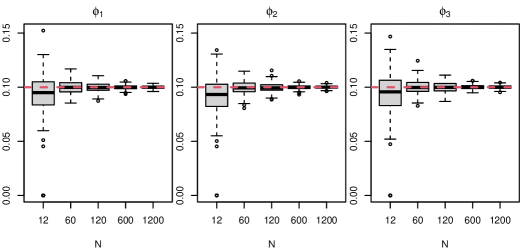
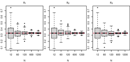
For this scenario, Figure 1 and Supplementary Tables 1 and 2 show that the EM estimates for $\phi_{k}$ and $\pi_{k}$, for $k=1,2,$ and 3, are centered around the true values across all the different choices of $N$, except for $\phi_{1},\phi_{2}$ and $\phi_{3}$ when $N=12$. Furthermore, as $N$ increases, the standard deviations of these estimates decrease as desired. Table 3 demonstrates that the MSE for estimating the $\lambda_{gk}$’s decreases while $N$ increases. Moreover, according to Supplementary Figure 2 , the clustering performance measured by the V-measures is deemed optimal (V-measure $=1$) except for the lowest value of $N=12$, which results in some misclassifications. Finally, we can see from Supplementary Figures 3 and 4 and Supplementary Tables 3 and 4 that although the computation time increases, as $N$ increases, the number of iterations until convergence decreases for the first three cases and then stabilizes for the larger $N$ cases.

Table 3: ZIP mixture model without covariates. Scenario 1: Mean squared error across genes and simulated datasets for the EM estimates of the $\lambda_{gk}$’s for each cluster $k$ and each $N$ according to the settings described in Table 2.

	$N$
$k$	12	60	120	600	1200
1	4.66910	0.58775	0.28343	0.05595	0.02819
2	4.18363	0.57776	0.28229	0.05559	0.02740
3	4.48772	0.57781	0.29115	0.05579	0.02800

Figure 1: ZIP mixture model without covariates. Scenario 1: Boxplots for the estimates of $\phi_{k}$ (top row) and $\pi_{k}$ (bottom row), for $k=1,\ldots,3$ obtained using the proposed EM algorithm across the datasets simulated from the settings described in Table 2. Red lines correspond to true values. See also Supplementary Tables 1 and 2 .

3.2.2 Scenario 2 – ZIP mixture model without covariates

In this scenario, the number of genes $G$ varies while the other parameters are kept fixed, as shown in Table 4. The number of clusters, the cluster assignment probabilities, the probabilities of always zero, and the $\lambda_{gk}$’s are fixed to values similar to those in Scenario 1. We fix $N=1200$ for this scenario, as seen in Table 4.

Table 4: ZIP mixture model without covariates. Scenario 2: Values chosen for the number of genes $G$ in each of five cases along with the fixed parameters used to simulate the datasets.

Case	$N$	$G$	$K$	$\phi_{k}$	$\pi_{k}$
1		12
2		60
3	1200	120	3	0.1	${}^{1}\!/_{K}$
4		600
5		1500

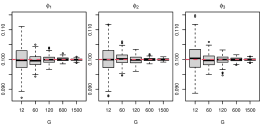
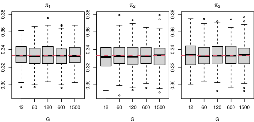
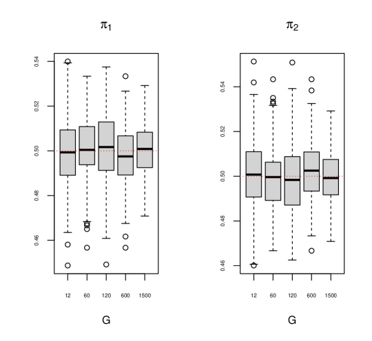
Figure 2 and Supplementary Table 5 show that as $G$ increases, the standard deviation of the estimates of each $\phi_{k}$ decreases, while the estimates remain centred around the true value of $0.1$. For the estimates of $\pi_{k}$, according to Figure 2 and Supplementary Table 6 , their standard deviations remain somewhat the same when varying $G$ across clusters. In addition, estimates of $\pi_{k}$ are unbiased, as in Scenario 1. Table 5 shows that the MSE of the estimates of the $\lambda_{gk}$’s for each cluster remains almost the same while varying $G$. Furthermore, the resulting V-measure values (Supplementary Figure 5 ) are equal to one for $G=60,120,600,1500$. However, for $G=12$, a few misclassifications lead to V-measure values slightly less than one. The number of iterations remains constant (see Table 7 and Figure 6 in the Supplementary Material), and the total computing time increases as $G$ increases (see Table 8 and Figure 7 in the Supplementary Material).

Table 5: ZIP mixture model without covariates. Scenario 2: Mean squared error across genes and simulated datasets for the EM estimates of the $\lambda_{gk}$’s for each cluster $k$ and each $G$ according to the settings described in Table 4.

	$G$
$k$	12	60	120	600	1500
1	0.02826	0.02804	0.02796	0.02823	0.02792
2	0.02823	0.02838	0.02794	0.02799	0.02810
3	0.02804	0.02879	0.02777	0.02791	0.02792

Figure 2: ZIP mixture model without covariates. Scenario 2: Boxplots for the estimates of $\phi_{k}$ (top row) and $\pi_{k}$ (bottom row), for $k=1,\ldots,3$ obtained using the proposed EM algorithm across the datasets simulated from the settings described in Table 4. Red lines correspond to true values. See also Supplementary Tables 5 and 6.

3.3 Simulation results for the ZIP mixture model with a size factor

In the simulation scenarios of this section, we model the rate parameter (expected read count) via a log link function as $\log(\lambda_{ngk})=\log(T_{n})+\beta_{0g}+\rho_{gk}$, which was introduced earlier in Section 2.1.2. So, to simulate data for the scenarios described in the following subsections, we construct the rate parameter by simulating the size factors, $T_{n}$, for $n=1\ldots,N$, from a normal distribution with parameters $\mu=1000$, $\sigma=100$, and we fix $\beta_{0g}$ at a value of one for all genes. For most of the cases, we choose three distinct values ($-0.6$, 0 and 0.6) for the cluster effects ($\rho_{gk}$’s), and we repeat the same value for a third of the number of genes in each cluster (i.e., $\frac{G}{3}$ times), in a way that the rate parameters for each gene are distinct across clusters. Note that, to avoid identifiability issues, we consider the restriction of $\sum_{k=1}^{K}\rho_{gk}=0$ to select the values of $\rho_{gk}$.

In this section, we study six different scenarios, each with 256 simulated datasets. Scenarios 1, 2, and 3 involve varying the values of $N$, $G$, and $K$, respectively. In Scenario 4, we consider two cases: Case 1 has initial parameter values matching the true values used to generate the data, while Case 2 has initial parameter values obtained through $K$-means clustering. Scenario 5 focuses on different probabilities of cluster assignments, while Scenario 6 varies the probabilities of always zero and compares the results. Note that, except for Case 2 in Scenario 4, we set the initial parameter values to the true values to speed up computation, as we did in Section 3.2.

In Sections 3.3.1 and 3.3.2, we present the simulation results for Scenarios 1 and 2, respectively. Results from Scenarios 3 to 6 are available in Sections 1.4.3 through 1.4.6 of the Supplementary Material.

3.3.1 Scenario 1 – ZIP mixture model with a size factor

In this scenario, similar to the case without covariates in Section 3.2.1, we vary $N$ while all other parameters and hyperparameters are kept fixed. See Table 6 for the parameter setting used to generate data under this scenario.

Table 6: ZIP mixture model with a size factor. Scenario 1: Values chosen for the number of observations $N$ in each case along with the fixed parameters used to simulate the datasets.

Case	$N$	$G$	$K$	$\phi_{k}$	$\pi_{k}$
1	12
2	60
3	120	120	3	0.1	${}^{1}\!/_{K}$
4	600
5	1200

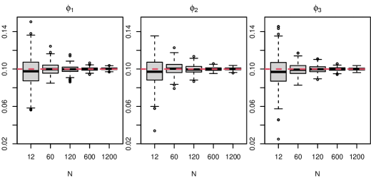
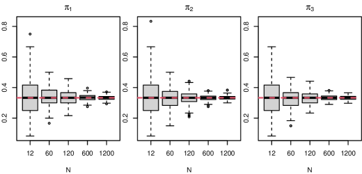
Figure 3 and Supplementary Tables 33 and 34 show that estimated probabilities of always zero ($\hat{\phi}_{k}$) and estimated cluster assignment’s probabilities ($\hat{\pi}_{k}$) are approximately around their true values and as $N$ increases, their standard deviations decrease. For the estimated $\rho_{gk}$ and $\beta_{0g}$, we consider the median absolute deviation (MAD) and we can observe from Tables 7 and 8 that as $N$ increases, the MADs for both $\rho_{gk}$ and $\beta_{0g}$ decrease. For most cases, the V-measures are one (see Supplementary Figure 22 ), except for the case with $N=12$ where there is some misclassification. As expected, the computing times increases while $N$ increases (see Table 35 and Figure 23 in the Supplementary Material). Finally, the required number of iterations to achieve convergence decreases as $N$ grows (see Table 36 and Figure 24 in the Supplementary Material).

Figure 3: ZIP mixture model with a size factor. Scenario 1: Boxplots for the estimates of $\phi_{k}$ (top row) and $\pi_{k}$ (bottom row), for $k=1,\ldots,3$ obtained using the proposed EM algorithm across the datasets simulated from the settings described in Table 6. Red lines correspond to true values. See also Supplementary Tables 33 and 34 .

Table 7: ZIP mixture model with a size factor. Scenario 1: Median absolute deviation for the estimates of $\rho_{gk}$ for each $k$ and each $N$, using the EM algorithm across the datasets simulated from the settings described in Table 6.

	$N$
$k$	12	60	120	600	1200
1	0.112408550	0.045393355	0.031839327	0.014172495	0.009948854
2	0.112812275	0.044446965	0.031538945	0.014278217	0.010051250
3	0.115637525	0.045467278	0.031932817	0.014086308	0.010112260

Table 8: ZIP mixture model with a size factor. Scenario 1: Median absolute deviation for the estimates of $\beta_{0g}$ for each $N$, using the EM algorithm across the datasets simulated from the settings described in Table 6.

$N$	12	60	120	600	1200
$\beta_{0g}$	0.08286	0.03281	0.02255	0.01017	0.00729

3.3.2 Scenario 2 – ZIP mixture model with a size factor

For this scenario, the number of genes $G$ varies as $G=12,\,60,\,120,\,600,\,1200,\,6000$ while all other parameters and hyperparameters are kept fixed according to the setting in Table 9.

Table 9: ZIP mixture model with a size factor. Scenario 2: Values chosen for the number of genes $G$ in each case along with the fixed parameters used to simulate the datasets.

Case	$N$	$G$	$K$	$\phi_{k}$	$\pi_{k}$
1		12
2		60
3	1200	120	3	0.1	${}^{1}\!/_{K}$
4		600
5		1200
6		6000

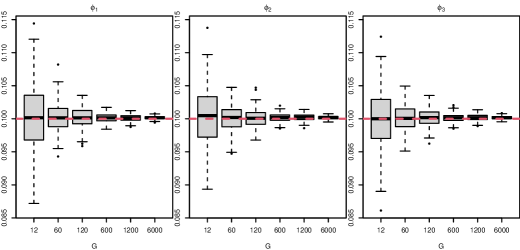
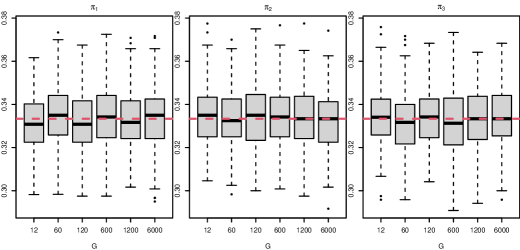
In this scenario, as can be seen in Figure 4 and Supplementary Tables 37 and 38 , estimates of $\phi_{k}$ and $\pi_{k}$ are approximately around their true values. Standard deviations decrease as $G$ increases for the probability of always zero ($\phi_{k}$). However, the standard deviations remain almost the same for the cluster assignment probabilities ($\pi_{k}$) as $G$ increases. Again, as expected, the MSEs for $\rho_{gk}$ and $\beta_{0g}$ remain somewhat the same in all cases (Tables 10 and 11). According to Supplementary Table 39 and Supplementary Figure 25 , for all cases, the number of EM iterations is between $7$ to $9$. The computation times increase for cases $5$ and $6$ which contain more genes (see Table 40 and Figure 26 in the Supplementary Material). Except for the first case with $G=12$, which has some misclassification leading to $V$-measures slightly less than one, for all other cases, the V-measures are equal to one (Supplementary Figure 27 ).

Figure 4: ZIP mixture model with a size factor. Scenario 2: Boxplots for the estimates of $\phi_{k}$ (top row) and $\pi_{k}$ (bottom row), for $k=1,\ldots,3$ obtained using the proposed EM algorithm across the datasets simulated from the settings described in Table 9. Red lines correspond to true values. See also Supplementary Tables 37 and 38.

Table 10: ZIP mixture model with a size factor. Scenario 2: Mean squared error for the estimates of $\rho_{gk}$ for each $k$ and each $G$, using the EM algorithm across the datasets simulated from the settings described in Table 9.

	$G$
$k$	12	60	120	600	1200	6000
1	0.000242605	0.000238823	0.000236353	0.000234922	0.000235966	0.000236160
2	0.000233509	0.000239676	0.000238435	0.000236828	0.000234413	0.000235708
3	0.000238199	0.000237094	0.000236564	0.000235157	0.000235041	0.000235893

Table 11: ZIP mixture model with a size factor. Scenario 2: Mean squared error for the estimates of for each $G$, using the EM algorithm across the datasets simulated from the settings described in Table 9.

$G$	12	60	120	600	1200	6000
$\beta_{0g}$	0.000115021	0.000114548	0.000112108	0.000113132	0.000113452	0.000114123

3.4 Simulation scenarios for the ZINB mixture model without covariates

In this section, we simulate data from the zero-inflated negative binomial mixture model without covariates (Section 2.2.1). We consider two scenarios where the number of cells ($N$) varies in Scenario 1, and in Scenario 2, the number of genes ($G$) varies while holding all other parameters and hyperparameters fixed. For both scenarios, we simulate data from $K=2$ clusters with equal cluster assignment probabilities ($\pi_{1}=\pi_{2}=0.5$). The probabilities of always zero are equal to $0.1$ for both clusters ($\phi_{1}=\phi_{2}=0.1$). The size parameters for the negative binomial components are $\nu_{1}=5$ and $\nu_{2}=20$. For the negative binomial rate parameters, we considered $\mu_{g1}=\mu_{1}=5$ and $\mu_{g2}=\mu_{2}=10$ for all $g$.

3.4.1 Scenario 1 – ZINB mixture model without covariates

As mentioned above, for this scenario, the number of cells ($N$) varies while we fix $G=120$ and all other parameters and hyperparameters according to the setting in Table 12.

Table 12: ZINB mixture model without covariates. Scenario 1: Values chosen for the number of observations $N$ in each case along with the fixed parameters used to simulate the datasets.

Case	$N$	$G$	$K$	$\phi_{k}$	$\pi_{k}$
1	60
2	120
3	300	120	2	0.1	${}^{1}\!/_{K}$
4	600
5	1200

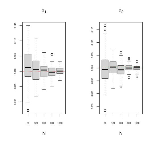
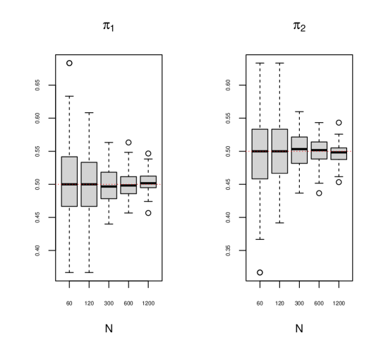
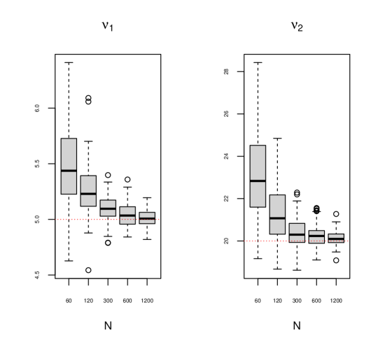
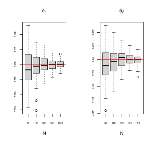
We can observe from Figure 5 and Supplementary Tables 81 and 82 that the estimates of $\pi_{k}$ and $\phi_{k}$ are close to their true values, and as $N$ increases, the standard deviations decrease. The MSEs for the estimates of the rate parameters decrease as $N$ increases (see Table 13). Furthermore, as shown in Figure 6 and Supplementary Table 83, for both clusters, the bias and the variance in the estimation of the size parameter decrease as $N$ increases. Finally, computing time increases when $N$ increases (see Table 84 and Figure 46 in the Supplementary Material), and V-measures for all data sets are equal to one.

Figure 5: ZINB mixture model without covariates. Scenario 1: Boxplots for the estimates of $\phi_{k}$ (top row) and $\pi_{k}$ (bottom row) using the EM algorithm across the datasets simulated from the settings described in Table 12. Red lines correspond to true values. See also Supplementary Tables 81 and 82.

Figure 6: ZINB mixture model without covariates. Scenario 1: Boxplots for the estimates of $\nu_{k}$ using the EM algorithm across the datasets simulated from the settings described in Table 12. Red lines correspond to true values. See also Supplementary Table 83.

Table 13: ZINB mixture model without covariates. Scenario 1: Mean squared error for the estimates of $\mu_{gk}$ for each $k$ and each $N$, using the EM algorithm across the datasets simulated from the settings described in Table 12.

	$N$
$k$	$60$	$120$	$300$	$600$	$1200$
1	0.40832	0.19947	0.08136	0.03927	0.01948
2	0.57480	0.27671	0.11284	0.05625	0.02844

3.4.2 Scenario 2 – ZINB mixture model without covariates

For this scenario, by fixing $N=1200$ and all other parameters and hyperparameters, the number of genes ($G$) varies between the simulated data according to the setting in Table 14.

Table 14: ZINB mixture model without covariates. Scenario 2: Values chosen for the number of genes $G$ in each case along with the fixed parameters used to simulate the datasets.

Case	$N$	$G$	$K$	$\phi_{k}$	$\pi_{k}$
1		12
2		60
3	1200	120	2	0.1	${}^{1}\!/_{K}$
4		600
5		1500

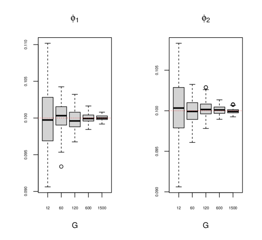
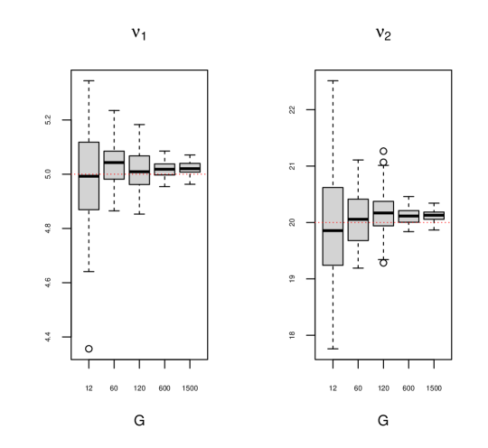
We can see from Figure 7 and Supplementary Tables 85 and 86 that the estimates for both parameters $\pi_{k}$ and $\phi_{k}$ are close to their true values. The standard deviation of the parameter estimates $\phi_{k}$ decreases as $G$ increases, but the standard deviations for the estimates of $\pi_{k}$ remain nearly the same with varying $G$. Table 15 shows that there are no significant changes in the MSEs of the parameter estimates of $\mu_{gk}$ for each cluster when $G$ varies. Furthermore, from Figure 8 and Supplementary Table 87, we can see that the size parameters are estimated close to their true values with a decrease in their standard deviations as $G$ increases. According to Table 88 and Figure 47 in the Supplementary Material, the computing time increases as $G$ increases. Finally, except for some misclassifications in the simulated data sets when $G=12$, the V-measures are very close to one for all the other cases (see Supplementary Figure 48).

Figure 7: ZINB mixture model without covariates. Scenario 2: Boxplots for the estimates of $\phi_{k}$ (top row) and $\pi_{k}$ (bottom row) using the EM algorithm across the datasets simulated from the settings described in Table 14. Red lines correspond to true values. See also Supplementary Tables 85 and 86.

Table 15: ZINB mixture model without covariates. Scenario 2: Mean squared error for the estimates of $\mu_{gk}$ for each $k$ and each $G$, using the EM algorithm across the datasets simulated from the settings described in Table 14.

	$G$
$k$	$12$	$60$	$120$	$600$	$1500$
1	0.02049	0.01917	0.01959	0.01990	0.01976
2	0.02816	0.02798	0.02851	0.02761	0.02783

Figure 8: ZINB mixture model without covariates. Scenario 2: Boxplots for the estimates of $\nu_{k}$ using the EM algorithm across the datasets simulated from the settings described in Table 14. Red lines correspond to true values. See also Supplementary Table 87.

3.5 Simulation scenarios for the ZINB mixture model with a size factor

In this section, we simulate only one scenario for the case of ZINB mixture model with a size factor when the number of cells varies as $N=60,120,300,600,$ and $1200$. We choose $G=120$ as the number of genes and $K=2$ as the number of clusters. We simulate $S=100$ datasets, and the true values of the parameters and hyperparameters are set as follows:

• $\pi=(0.5,0.5)$;

• $\phi=(0.1,0.2)$;

• $T_{n}\mbox{'s}$ are generated from a normal distribution with $\mu=10$ and $\sigma=0.5$;

• $\beta_{0g}=0.85$ for all $g$;

• $\rho_{1g}=(2,\dots,2,-2,\dots,-2)$, and $\rho_{2g}=(-2,\dots,-2,2,\dots,2)$.

Note that, for the cluster effect parameters ($\rho_{gk}$’s), over each cluster, the first half of the genes are assigned one value (either $2$ or $-2$), and the remaining half is assigned another value (either $2$ or $-2$) in such a way that their sums are equal to zero. The setting for this simulation scenario is also shown in Table 16.

Table 16: ZINB mixture model with a size factor. Scenario 1: Values chosen for the number of observations $N$ in each case along with the fixed parameters used to simulate the datasets.

Case	$N$	$G$	$K$	$\phi_{k}$	$\pi_{k}$
1	60
2	120
3	300	120	2	($\phi_{1}=0.1$,$\phi_{2}=0.2$)	${}^{1}\!/_{K}$
4	600
5	1200

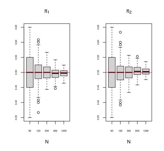
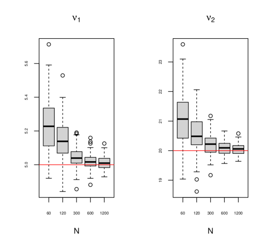
In Figure 9 and Supplementary Table 89, we can see that the estimated cluster assignment probabilities ($\hat{\pi}_{k}$) are close to their true values, and their standard deviations decrease as $N$ increases. From Figure 9 and Supplementary Table 90, we can observe similar behaviour for the estimated probabilities of always zero ($\hat{\phi}_{k}$); that is, as $N$ increases, their standard deviations decrease, and their values are close to the true values. Tables 17 and 18 present the MSEs for the estimated values of $\rho_{gk}$ and $\beta_{0g}$. We can observe that the MSEs reduce as $N$ becomes larger for both parameters. Figure 10 and Supplementary Table 91 illustrate the behavior of the estimated size parameters ($\nu_{1}$ and $\nu_{2}$). As expected, the estimated values of $\nu_{1}$ and $\nu_{2}$ get closer to their true values, and their standard deviations decrease as the sample size ($N$) increases. In all cases, the V-measures are equal to one, indicating perfect clustering assignment results. Finally, Supplementary Table 92 and Supplementary Figure 49 show that the computing time increases as $N$ increases.

Figure 9: ZINB mixture model with a size factor: Boxplots for the estimates of $\phi_{k}$ (top row) and $\pi_{k}$ (bottom row) using the EM algorithm across the datasets simulated from the settings described in Table 16. Red lines correspond to true values. See also Supplementary Tables 89 and 90.

Figure 10: ZINB mixture model with a size factor: Boxplots for the estimates of $\nu_{k}$ using the EM algorithm across the datasets simulated from the settings described in Table 16. Red lines correspond to true values. See also Supplementary Table 91 .

Table 17: ZINB mixture model with a size factor: Mean Squared error (MSE) for the estimates of $\rho_{gk}$ for each $k$ and each $N$, using the EM algorithm across the datasets simulated from the settings described in Table 16.

	$N$
$k$	$60$	$120$	$300$	$600$	$1200$
1	0.08710	0.06189	0.04038	0.02848	0.01996
2	0.04873	0.03532	0.02200	0.01585	0.01127

Table 18: ZINB mixture model with a size factor: Mean squared error (MSE) for the estimates of $\beta_{0g}$ for each $N$, using the EM algorithm across the datasets simulated from the settings described in Table 16.

$N$	$60$	$120$	$300$	$600$	$1200$
$\beta_{0g}$	0.04207	0.02902	0.01791	0.01278	0.00935

4 Data Analysis

In this Section, we illustrate the utility of our proposed model-based clustering methods introduced in Section 2 by applying them to two publicly available datasets. In Section 4.1, we consider scRNA-seq data from mouse embryonic stem cells collected by Klein et al. (2015) and fit the ZIP mixture model without covariates as well as the ZIP mixture model with a size factor. In Section 4.2, we analyze scRNA-seq data from mouse liver tissue cells profiled by Han et al. (2018) using the ZIP mixture model without covariates and the ZINB mixture without covariates.

4.1 Mouse Embryonic Stem Cell (MESC) data

Klein et al. (2015) developed a laboratory platform (called inDrop from indexing Droplets) for indexing thousands of individual cells for RNA sequencing. Klein et al. then used inDrop to obtain single-cell RNA sequencing data from mouse embryonic stem cells before (day 0) and after leukemia inhibitory factor (LIF) withdrawal (days 2, 4, and 7). Read counts across cells and genes for the different experiment days in Klein et al. (2015) are publicly available through the Gene Expression Omnibus online repository under the accession code GSE65525.

For our analysis, we consider the pooled data for day $0$ ($933$ cells) and day $4$ ($683$ cells) for a total of $N=$1616$$ cells and $G=$24175$$ genes. Then, as a common step in the analysis of scRNA-seq data (Zeisel et al., 2015; Klein et al., 2015; Jovic et al., 2021), we filter out genes with very little variation across cells. In particular, we filter out genes with a read count interquartile range across cells smaller than one ($\mbox{IQR}=Q_{3}-Q_{1}\leq 1$), resulting in $4514$ genes initially selected. From these $4514$ genes, we select $100$ of them with the highest read count standard deviations across cells. Therefore, we continue the data analysis in this section using the read count data for $N=$1616$$ cells and the selected $G=100$ most variable genes. Note that our choice to select 100 genes was based on reducing the computation complexity of running different models for different number of clusters with different initializations. However, one can consider a larger number of genes and compare the results.

We fit the mouse embryonic stem cell data (MESC) data considering the ZIP mixture model without covariates (Section 2.1.1) and with a size factor (as the total number of read counts for each cell before performing any gene filtering) as shown in Equation (20) of Section 2.1.2. For each model, we apply the proposed EM algorithm considering different choices of $K$ (total number of clusters) and two clustering initialization methods: $K$-means and random clustering. After obtaining initial cluster assignments for the cells by $K$-means or random clustering, we can find the initial parameter values required to start the EM algorithm as follows. For the cluster probabilities, the $\pi_{k}$’s, we set their initial values to the proportion of cells assigned to each initial cluster. For the probabilities of always zero, the $\phi_{k}$’s, we set each $\phi_{k}^{(0)}$ to the proportion of zero entries in each cluster. For the case of the ZIP mixture model without covariates (simple ZIP model), for each initial cluster, we take the mean read count for each gene as the initial values of the $\lambda_{gk}$’s. For the ZIP mixture model with a size factor, we initialize the $\beta_{0g}$’s at zero, and the cluster effects, the $\rho_{gk}$’s, as the mean read count for each gene for each initial cluster.

For each choice of $K$ and each initialization method (random or $K$-means), we run the EM algorithm $32$ times corresponding to $32$ different initialization runs from different seeds. Next, for each initialization method, we choose the run with the smallest Aikaike Information Criterion (AIC) for each possible total number of clusters $K$. For each initialization method, after choosing the best run over each $K$, we use the elbow method to select the optimum number of clusters. The elbow takes the point with the highest AIC (on the $y$-axis) and the point with the highest $K$ (in the $x$-axis) and defines a line, usually going from the top-left to the bottom-right on the plot. The optimum point is then determined to be the one that is the farthest away below this line.

4.1.1 Results of fitting the ZIP mixture model without covariates to the MESC data

This section presents the results of fitting the ZIP mixture model without covariates (simple ZIP, Section 2.1.1) to the MESC dataset. As mentioned above, for our analysis, we use the pooled data of day $0$ and day $4$ over the $100$ most variable selected genes and $1616$ cells.

Supplementary Figures 50 and 51 show the smallest AIC over the 32 EM runs for each $K$ when considering random and $K$-means initialization methods, respectively. Based on the elbow method, both initialization methods lead to $K=4$ as the best number of clusters for the simple ZIP model. Next, as a final choice between these two results with $K=4$, one using random clustering initialization and the other $K$-means, we select the one with the lowest AIC. In this case, the AIC from the $K$-means initialization approach reaches a lower value than that of the random initialization. Therefore, we select the EM run with the best AIC for $K=4$ from the $K$-means initialization approach and present its results in what follows.

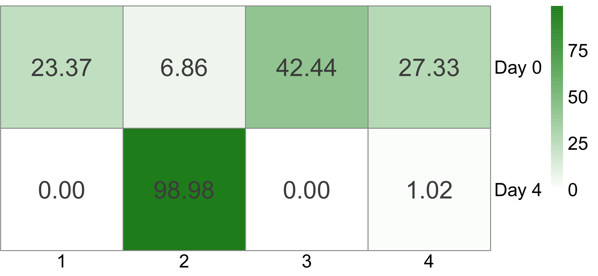
Figure 11 and Supplementary Table 93 present the co-clustering plot and confusion matrix, respectively, between cell experiment days (day 0 and day 4) and the inferred cell clusters (1, 2, 3, and 4) for the best EM algorithm run with $K=4$. The co-clustering plot allows us to observe the percentage of cells from each experiment day present in each inferred cluster. We can see that most cells (approximately $99\%$) of day $4$ are present in the inferred cluster $2$ and cells from day $0$ fall mainly into the inferred clusters $1$, $3$, and $4$. Interestingly, Klein et al. (2015) found in their analyses that cells from day $0$ belong to three main subpopulations plus two other rare subpopulations when clustering only day $0$ cells via hierarchical clustering.

Table 19 shows the estimated cluster proportion, $\hat{\pi}_{k}$, for each inferred cluster. Cluster $2$ has the highest proportion of cell assignments ($\hat{\pi}_{2}=45.91\%$) compared to the other three clusters. The estimated probability of always zero for each cluster is also displayed in Table 19 with cluster $2$ showing the highest probability at $\hat{\phi}_{2}=1.191\%$. Figure 12 shows the heatmap of the rate parameter estimates ($\hat{\lambda}_{gk}$’s) for each cluster (rows) over the $100$ genes (columns) when fitting the ZIP simple model to the MESC data.

Supplementary Figure 52 shows the heatmap of the data (read counts across all $1616$ cells and all $100$ selected genes) with cells (rows) ordered by their inferred cluster assignments. The heatmap also contains annotation for each cell’s experiment day (0 or 4). Supplementary Figure 53 presents a dimensionality reduction visualization of the data using $t$-SNE (Van der Maaten and Hinton, 2008). In the $t$-SNE plot, circle and triangle points correspond to cells from day 0 and day 4, respectively, and the colours to the inferred four clusters. Moreover, Supplementary Figure 54 shows the cluster assignment expected values (or probabilities), i.e., the $\hat{Z}_{nk}$’s, which we used to determine the final inferred cluster assignment of each cell. We can observe that overall the proposed EM algorithm assigned cells to their clusters with high (close to 1) probabilities.

Figure 11: MESC dataset. Co-clustering between experiment days (0 and 4; rows) and inferred clusters by the proposed EM algorithm (1, 2, 3, and 4; columns). Each entry $a_{ij}$ represents the $\%$ of cells from day $i$ that are present in the inferred cluster $j$. Rows sum up to $100\%$. Inferred clusters are from the best EM algorithm run ($K$-means initialization and $K=4$) under the simple ZIP model.

Table 19: Estimates of $\pi_{k}$ and $\phi_{k}$ for the MESC dataset obtained from the best EM algorithm run ($K$-means initialization and $K=4$) under the simple ZIP model.

$k$	$\hat{\pi}_{k}$	$\hat{\phi}_{k}$
1	0.13599	0.00077
2	0.45910	0.01191
3	0.24507	0.00077
4	0.15984	0.00127

Figure 12: Heatmap of the $\hat{\lambda}_{gk}$’s for MESC data set obtained from the best EM algorithm run ($K$-means initialization and $K=4$) under the simple ZIP model. Each row corresponds to a cluster, and each column to a gene. Dark blue colours represent low values, and dark red colours represent high values of $\hat{\lambda}_{gk}$.

4.1.2 Results of fitting the ZIP mixture model with a size factor to the MESC data

In this section, we present the results of fitting the ZIP mixture model with a size factor (as shown in Equation (20) of Section 2.1.2) to the same MESC dataset analyzed in Section 4.1.1; that is, the pooled data of day $0$ and day $4$ over the $100$ most variable selected genes and $1616$ cells.

Supplementary Figures 55 and 56 show the smallest AIC for each $K$ for random and $K$-means initialization methods, respectively. Based on the elbow method, the random initialization approach leads to $K=6$ clusters as the best number of clusters for the ZIP mixture model with size factor; however, the $K$-means initialization method leads to $K=4$ as the optimum number for clusters. As a final choice, we choose the best number of clusters between these two initialization methods based on the lowest AIC. Thus, as $K$-means initialization leads to the smallest AIC value, we choose the EM run with the best AIC from the $K$-means method when $K=4$ and present its results in the following.

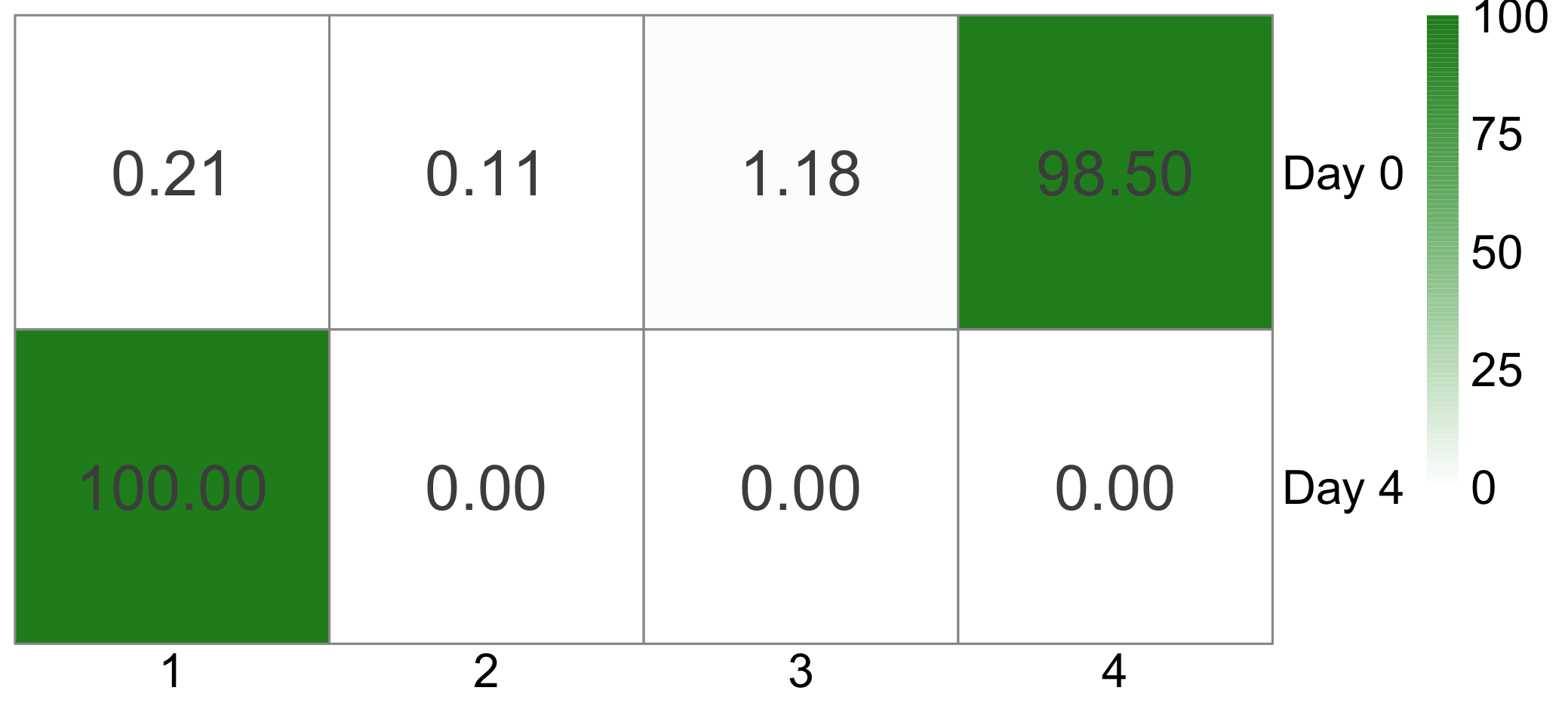
Figure 13 and Supplementary Table 94 display the co-clustering plot and confusion matrix, respectively, between cell experiment days ($0$ and $4$) and the inferred four clusters from the best EM algorithm run ($K=4$ clusters and $K$-means clustering initialization method) under a ZIP mixture model with a size factor. Notably, all cells ($100\%$) from day $4$ are present in the inferred cluster $1$, while most cells (approximately $98.5\%$) from day $0$ are in the inferred cluster $4$. Only a small portion of cells from day $0$ are found in the other inferred clusters: $0.21\%$ in cluster $1$, $0.11\%$ in cluster $2$, and $1.18\%$ in cluster $3$. Interestingly, these clustering results are similar to the ones presented in Qi et al. (2020).

The estimated cluster proportions ($\hat{\pi}_{k}$’s) are presented in Table 20. We can observe that more than $50\%$ of the cells belong to cluster $4$ ($56.83\%$), and $42.4\%$ of the cells fall into cluster $1$ and only a few of them are assigned to the other two clusters. Table 20 also shows the estimated probability of always zero for each cluster $k$, and we can see that $\hat{\phi}_{1}=0.01415$ has the highest probability of always zero compared with the other clusters. Figure 14 shows the heatmap of the estimates of $\beta_{0g}$ (baseline expression) and $\rho_{gk}$ (cluster effect) over the $100$ genes (columns) when fitting the ZIP mixture model with a size factor. The $\hat{\beta}_{0g}$’s are shown in the first row, and the $\hat{\rho}_{gk}$’s for each cluster $k$ are presented in rows $2$ to $5$.

Similarly to the previous section, Supplementary Figure 57 shows the heatmap of the read counts across all $1616$ cells and all $100$ selected genes with cells (rows) ordered by their inferred cluster assignments from the ZIP mixture model with size factor. The heatmap also shows each cell’s experiment day ($0$ or $4$). Supplementary Figure 58 shows the $t$-SNE representation of the data in two dimensions, where circle and triangle points correspond to cells from day 0 and day 4, respectively, and the colours to the inferred four clusters. As in Section 4.1.1, we can observe in Supplementary Figure 59 that overall the proposed EM algorithm assigned cells to their clusters with high (close to $1$) probabilities.

Figure 13: MESC dataset. Co-clustering between experiment days (0 and 4; rows) and inferred clusters by the proposed EM algorithm (1, 2, 3, and 4; columns). Each entry $a_{ij}$ represents the $\%$ of cells from day $i$ that are present in the inferred cluster $j$. Rows sum up to $100\%$. Inferred clusters are from the best EM algorithm run ($K$-means initialization and $K=4$) under the ZIP mixture model with a size factor.

Table 20: Estimates of $\pi_{k}$ and $\phi_{k}$ for the MESC dataset obtained from the best EM algorithm run ($K$-means initialization and $K=4$) under the ZIP mixture model with size factor.

$k$	$\hat{\pi}_{k}$	$\hat{\phi}_{k}$
1	0.42384	0.01415
2	0.00062	0.00000
3	0.00727	0.00086
4	0.56828	0.00072

Figure 14: Heatmap of the $\hat{\beta}_{0g}$’s and $\hat{\lambda}_{gk}$’s for the MESC dataset obtained from the best EM algorithm run ($K$-means initialization and $K=4$) under the ZIP mixture model with size factor. $\hat{\beta}_{0g}$’s are shown in the first row, and the $\hat{\rho}_{gk}$’s for each cluster $k$ are presented in rows $2$ to $5$. The columns correspond to the 100 selected genes. Dark blue colours represent low values, and dark red colours represent high values of $\hat{\beta}_{0g}$ and $\hat{\rho}_{gk}$.

4.1.3 Model selection for the MESC dataset

Table 21 shows the AIC values obtained from the best EM algorithm runs when fitting the simple ZIP model (ZIP mixture model without covariates) and the ZIP mixture model with a size factor. These values correspond to the red points in Supplementary Figures 51 and 56 . Table 21 shows that the ZIP mixture model with a size factor leads to a smaller AIC value than the simple ZIP model. Therefore, the ZIP mixture model with a size factor fits the MESC data better than the ZIP simple model. As shown in Section 4.1.2, the selected ZIP mixture model with size factor resulted in two main clusters, one with cells from day 0 and the other with cells from day 4.

Table 21: AIC values corresponding to the best EM runs when fitting the simple ZIP model and the ZIP mixture model with size factor to the MESC dataset (see also Supplementary Figures 51 and 56 ).

Model	AIC
Simple ZIP	80274.22
ZIP mixture model with size factor	72544.74

4.2 Liver Data

Han et al. (2018) collected thousands of single-cell transcriptome profiles from several mouse tissues, organs, and cell cultures using Microwell-seq as a high-throughput and low-cost scRNA-seq platform. The data is publicly available at https://figshare.com/s/865e694ad06d5857db4b and in the Gene Expression Omnibus online repository under the accession code GSE108097. In this paper, we focus on a subset of the scRNA-seq data from mouse liver tissue provided by Han et al. (2018), which comprises a total of $N=$4685$$ cells and $G=$15491$$ genes. We first select $N=$1000$$ cells from the total $4685$ cells using random sampling. Then, as in Section 4.1, we filter out genes with minimal variation across these randomly selected cells, keeping only a set of highly variable genes. In particular, we choose $100$ genes with the highest standard deviations of read count across cells. Therefore, the data analysis results presented in this section are based on the randomly selected $1000$ cells and their corresponding $100$ highly variable genes of the liver tissue data in Han et al. (2018), which will be referred to as the liver data hereafter.

We fit the liver data considering the ZIP mixture model without covariates (simple ZIP, Section 2.1.1) and the ZINB mixture model without covariates (simple ZINB, Section 2.2.1) via the EM algorithm. Similarly to Section 4.1, we apply the proposed EM algorithm to the liver data considering different choices of $K$ (total number of clusters) and two clustering initialization approaches: $K$-means and random clustering. After obtaining the initial cluster assignments for the cells using the two initialization methods, we can find the initial starting points of the EM algorithm for each model fitting. We can obtain the starting points for the cluster probabilities ($\pi_{k}$’s), proportions of always zero in each cluster ($\phi_{k}$’s) for both the simple ZIP and ZINB mixture models and the rate parameters of simple ZIP model as described earlier in Section 4.1. The initial rate parameters for each cluster under the simple ZINB mixture model are the mean read counts for each gene across cells in each initial cluster (similar to the initial rates for the simple ZIP mixture model). Finally, we calculate the initial values for the size parameters ($\nu_{k}$’s) for the simple ZINB mixture model. For each $k$, first, we calculate $\mu_{k}$ and $\sigma_{k}$ as the mean and standard deviation of read counts over all genes and cells in the initial cluster $k$. Then, we calculate the initial value for $\nu_{k}$ as:

$$\nu_{k}^{(0)}=\Big{[}\Big{(}\frac{\sigma_{k}}{\mu_{k}}\Big{)}^{2}-\frac{1}{\mu_{k}}\Big{]}^{-1}.$$

Again, similar to Section 4.1, for each choice of $K$ and initialization method, we run the proposed EM algorithm $32$ times as $32$ different initialization runs from different seeds and choose the run with the smallest AIC for each possible $K$ for each initialization method. Then, after selecting the best run for each $K$, we use the elbow method to find the optimum number of clusters $K$.

4.2.1 Result of fitting the ZIP mixture model without covariates to the liver data

This section presents the results of fitting the ZIP mixture model (simple ZIP) to the liver data set. The data correspond to the $1000$ randomly selected cells and the $100$ selected highly variable genes for our analysis.

Figures 60 and 61 in the supplementary show the smallest AIC for each $K$ for random and $K$-means initialization methods, respectively. Based on the elbow method, the random initialization approach leads to $K=6$ clusters as the best number of clusters. The $K$-means approach yields $K=4$ as the optimum number of clusters. As the best EM run from $K$-means initialization has the lowest value of AIC, in what follows, we present the results of the EM run with $K=4$ from the $K$-means initialization method.

Table 22 and Supplementary Figure 62 show the confusion matrix and co-clustering plot, respectively, between the cell type labels provided in the dataset by Han et al. (2018) and the inferred four clusters for the best EM run ($K=4$ clusters and $K$-means initialization approach) for the ZIP mixture model without covariates. We can observe that B cells ($62.16\%$) are mostly assigned to the inferred cluster $3$, dendritic cells are present equally in clusters $1$ ($50\%$) and $3$ ($50\%$), endothelial cells ($91.76\%$) are mainly assigned to cluster $3$, all epithelial cells are part of the inferred cluster $2$, $77.59\%$ of erythroblast cells and $84.62\%$ of granulocyte cells are assigned to cluster $3$, $90.14\%$ of hepatocyte cells are in the inferred cluster $2$, $67.14\%$ and $32.86\%$ of Kuppfer cells are assigned to clusters $1$ and $3$, respectively. $58\%$ of the macrophage cells are present in cluster $3$, and $42\%$ of them are in cluster $1$. All ($100\%$) of the neutrophil cells and $92.65\%$ of the T cells are assigned to the inferred cluster $3$.

Table 22: Confusion matrix between the EM clustering result when fitting the simple ZIP model to the liver data and the cell types. Inferred clusters are from the best EM algorithm run ($K$-means initialization and $K=4$) under the simple ZIP model (see also Supplementary Figure 62).

	Inferred cluster
Cell type	1	2	3	4
B cell	3	1	23	10
Dendritic cell	54	0	54	0
Endothelial cell	17	5	245	0
Epithelial cell	0	32	0	0
Erythroblast	9	17	90	0
Granulocyte	5	1	33	0
Hepatocyte	2	64	5	0
Kuppfer cell	141	0	69	0
Macrophage	21	0	29	0
Neutrophil	0	0	2	0
T cell	5	0	63	0

The estimated cluster proportions ($\hat{\pi}_{k}$’s) and probabilities of always zero ($\hat{\phi}_{k}$’s) are presented in Table 23. The table shows that $60.929\%$ of the cells are assigned in the inferred cluster $3$, $26.114\%$ are assigned to cluster $1$, $11.957\%$ fall into cluster $2$, and only $1\%$ of them fall into cluster $4$. We can also see that the higher estimated probabilities of always zero are for the inferred clusters $2$ and $4$, $\hat{\phi}_{2}=0.26895$ and $\hat{\phi}_{4}=0.13620$, respectively, followed by clusters $1$ and $3$ ($\hat{\phi}_{1}=0.09183$ and $\hat{\phi}_{3}=0.08780$). Finally, Figure 15 shows the heatmap of the estimates of the rate parameters ($\hat{\lambda}_{gk}$’s) for each cluster (rows) over the $100$ selected genes (columns) when fitting the ZIP simple model to the liver data.

Figure 63 in the Supplementary Material displays the heatmap of the read counts across the randomly selected $1000$ cells and all $100$ selected genes. The cells (rows) are ordered by their inferred cluster assignments from the simple ZIP mixture model. The heatmap also shows each cell’s type. Additionally, Supplementary Figure 64 shows the $t$-SNE representation of the data in two dimensions, where different point shapes correspond to the cell type and point colours to the inferred four clusters. As in Sections 4.1.1 and 4.1.2, Supplementary Figure 65 demonstrates that the proposed EM algorithm assigned cells to their clusters with high (close to $1$) probabilities.

Figure 15: Heatmap of the $\hat{\lambda}_{gk}$’s for the liver dataset obtained from the best EM algorithm run ($K$-means initialization and $K=4$) under the simple ZIP model. Each row corresponds to a cluster, and each column to a gene. Dark blue colours represent low values, and dark red colours represent high values of $\hat{\lambda}_{gk}$.

Table 23: Estimates of $\pi_{k}$ and $\phi_{k}$ for the liver dataset obtained from the best EM algorithm run ($K$-means initialization and $K=4$) under the simple ZIP model.

$k$	$\hat{\pi}_{k}$	$\hat{\phi}_{k}$
1	0.26114	0.09183
2	0.11957	0.26895
3	0.60929	0.08780
4	0.01000	0.13620

4.2.2 Result of fitting the ZINB mixture model without covariates to the liver data

In this section, the results of fitting the ZINB mixture model without covariates (simple ZINB) for the liver data (over the selected $1000$ cells and $100$ selected mostly variable genes, same data as in Section 4.2.1) are presented.

Supplementary Figures 66 and 67 present the corresponding smallest AIC for each $K$ for the random and $K$-means initialization methods, respectively. Based on the elbow method, random initialization results in $K=4$ as the optimum number of clusters, while $K$-means leads to $K=5$ as the best number of clusters. As the one from $K$-means clustering initialization has the smallest AIC, we choose that EM run for further analysis in this section. Therefore, for the simple ZINB mixture model, we choose the EM run with $K=5$ from the $K$-means initialization method, and we present its results in what follows.

Table 24 and Supplementary Figure 68 show the confusion matrix and co-clustering plot, respectively, between the cell types and the inferred five clusters for the best EM run ($K=5$ clusters and $K$-means initialization approach) for the ZINB mixture model without covariates. We can see that B cells are assigned primarily to $3$ clusters, with $43.24\%$ of them in cluster $3$, $35.14\%$ in cluster $5$, and $13.51\%$ in cluster $2$. Dendritic cells are primarily present in clusters $2$ ($85.19\%$), endothelial cells ($91.39\%$) are dense in cluster $3$, epithelial ($90.62\%$) cells are mainly in the inferred cluster $1$. $75\%$ of erythroblast cells and $69.23\%$ of Granulocyte cells fall into cluster $3$. $84.51\%$ of Hepatocyte cells are in the inferred cluster $1$, Kuppfer cells are mostly assigned to clusters $3$ and $4$, with $19.05\%$ and $80\%$, respectively. $70\%$ of macrophage cells fall into cluster $2$ and $22\%$ of them are in cluster $3$, and the remaining $8\%$ in cluster $4$. Neutrophil cells are assigned equally ($50\%$) to the inferred clusters $3$ and $5$. Finally, $77.94\%$ of T cells fall into the inferred cluster $3$.

Table 24: Confusion matrix between the EM clustering result when fitting the simple ZINB model to the liver data and the cell type labels. Inferred clusters are from the best EM algorithm run ($K$-means initialization and $K=5$) under the simple ZINB model (see also Supplementary Figure 68).

	Inferred cluster
Cell type	1	2	3	4	5
B cell	0	5	16	3	13
Dendritic cell	0	92	12	3	1
Endothelial cell	0	3	244	17	3
Epithelial cell	29	0	0	0	3
Erythroblast	1	3	87	9	16
Granulocyte	0	3	27	3	6
Hepatocyte	60	1	1	0	9
Kuppfer cell	0	2	40	168	0
Macrophage	0	35	11	4	0
Neutrophil	0	0	1	0	1
T cell	2	9	53	2	2

The estimated cluster proportions ($\hat{\pi}_{k}$’s) are presented in Table 25. We can see that $49.157\%$ of the cells are assigned to the inferred cluster $3$, $20.986\%$ are assigned to cluster $4$, $15.235\%$ fall into cluster $2$, $9.163\%$ are in cluster $1$, and only $5.54\%$ of them are assigned to cluster $5$. Table 25 also shows the estimated probability of always zero for each cluster $k$, and we can see that $\hat{\phi}_{1}=0.07266$ is the highest probability of always zero compared with the other clusters. The estimates of the size parameters for each cluster ($\nu_{k}$’s) are also shown in Table 25. We can see that clusters $3$, $4$, and $2$ have the higher estimated values ($\hat{\nu}_{3}=4.11696,\,\hat{\nu}_{4}=3.75589,\,\hat{\nu}_{2}=2.12675$), followed by the smaller estimated values for the other two clusters ($\hat{\nu}_{1}=1.93291,\,\hat{\nu}_{5}=0.66367$), demonstrating the presence of overdispersion in the liver data. Finally, Figure 16 shows the heatmap of the estimates of the rate parameters ($\hat{\mu}_{gk}$’s) for each cluster (rows) over the $100$ selected genes (columns) when fitting the ZINB simple model to the liver data.

Supplementary Figure 69 shows the heatmap of the read counts across the randomly selected $1000$ cells and all $100$ most variable selected genes with cells (rows) ordered by their inferred cluster assignment from the simple ZINB mixture model. The heatmap also shows the annotation for each cell’s type. Figure 70 in the Supplementary Material shows the $t$-SNE representation of the data in two dimensions, where different point shapes correspond to the cell type and the colors to the inferred five clusters. As in the previous sections, we can observe in Supplementary Figure 71 that overall the proposed EM algorithm assigned cells to their clusters with high (close to $1$) probabilities.

Figure 16: Heatmap of the $\hat{\mu}_{gk}$’s for the liver dataset obtained from the best EM algorithm run ($K$-means initialization and $K=5$) under the simple ZINB model. Each row corresponds to a cluster, and each column to a gene. Dark blue colours represent low values, and dark red colours represent high values of $\hat{\mu}_{gk}$.

Table 25: Estimates of $\pi_{k}$ for the liver dataset obtained from the best EM algorithm run ($K$-means initialization and $K=5$) under the simple ZINB model.

$k$	$\hat{\pi}_{k}$	$\hat{\phi}_{k}$	$\hat{\nu}_{k}$
1	0.09163	0.07266	1.93291
2	0.15235	0.00000	2.12675
3	0.49157	0.00005	4.11696
4	0.20986	0.00000	3.75589
5	0.05458	0.00007	0.66367

4.2.3 Model selection for the liver data

Table 26 shows the AIC values obtained from the best EM algorithm runs when fitting the simple ZIP model (ZIP mixture model without covariates) and the simple ZINB model (ZINB mixture model without covariates) to the liver data. These values correspond to the red points in Figures 61 and 67 in the Supplementary Material. Thus, based on the AIC values shown in Table 26, the simple ZINB model leads to a smaller AIC value than the simple ZIP model and, therefore, we can conclude that the simple ZINB fits the liver data better than the ZIP simple model. As shown in Section 4.2.2, the selected simple ZINB model resulted in five clusters comprising different cell types in the liver tissue.

Table 26: AIC values corresponding to the best EM runs when fitting the simple ZIP model and simpe ZINB model to the Liver dataset (see also Supplementary Figures 61 and 67).

Model	AIC
Simple ZIP	115744.1
Simple ZINB	360931

5 Conclusion

In this paper, we proposed a novel mixture-model-based clustering approach for scRNA-seq data. We conducted simulation studies to assess the frequentist properties (bias and variance) of the proposed parameter estimators. We also applied our clustering methodology on real publicly available scRNA-seq datasets.

In Section 2 of our paper, we introduced a new model-based approach for clustering scRNA-seq data, specifically addressing the issue of zero inflation in the data. Our proposed clustering algorithm is based on a mixture of zero-inflated Poisson (ZIP) or zero-inflated negative binomial (ZINB) distributions. We developed an EM algorithm to obtain cluster assignments and estimate the parameters for each proposed ZIP and ZINB mixture model with and without covariates. While other model-based clustering algorithms exist for this type of data, our approach directly considers the excess of zeros in the counts through our proposed probabilistic mixture models, which sets our study apart from previous work in this area.

In Section 3, we studied the performance of the proposed clustering algorithm on simulated data under various scenarios for each proposed mixture model. For the ZIP mixture model without covariates, we examined the estimation of the model parameters over six different scenarios, including varying the number of cells ($N$), the number of genes ($G$), the number of clusters ($K$), the probabilities of cluster assignments, the probabilities of always zero, and the rate parameters across clusters. We also studied parameter estimation for six scenarios under the ZIP mixture model with only a size factor. Changes in the number of cells, genes, and clusters were studied in Scenarios $1$, $2$, and $3$. In Scenario $4$, we studied the parameter estimation when we use true values as the initialization points compared to when we initialize the EM based on $K$-means clustering. Changes in the probabilities of cluster assignments were studied in Scenario $5$, and Scenario $6$ investigated changes in the probabilities of always zero. We also investigated parameter estimation for the ZIP mixture model with one covariate considering two scenarios, one varying the number of cells and another the number of genes (results available only in the Supplementary Material). Considering a ZINB mixture model without covariates, we conducted simulation studies varying the number of cells and the number of genes. Finally, we studied parameter estimation under the ZINB mixture model with a size factor when the number of cells varies.

Results from the simulation studies showed that for all of the estimated parameters, the bias, standard deviation, and MSE (or MAD) decreased as $N$ (the number of cells) increased, as expected from the convergence properties of the EM algorithm. When the number of genes ($G$) increased, in terms of bias, our proposed EM framework performed well, as almost all the estimated parameters were close to their true values. The standard deviations and MSEs (or MADs) for the estimated values of the cluster assignment probabilities and the rate parameters (for all models, including without covariates, with a size factor, and with covariates) remained almost the same when $G$ increased. However, when estimating the probability of always zero, we observed a decrease in standard deviation when increasing $G$. Furthermore, when increasing model complexity by increasing the number of clusters $K$, almost for all cases, the standard deviations, MSE, or MAD increased while all the estimates remained close to their true values.

In Section 4, we applied the proposed models and developed EM algorithms to the MESC and liver datasets. For the MESC data, we considered and compared the results from the ZIP mixture models without covariates and with a size factor. Using the AIC criterion for comparing the models, we selected the ZIP mixture model with a size factor as the final choice, resulting in $K=4$ clusters, which clustered cells mainly in $2$ clusters (all cells from experiment day $4$ were assigned to cluster $1$ and $98.5\%$ of the cells from experiment day $0$ were assigned to cluster $4$). Next, we fitted the simple ZIP and ZINB models (i.e., without covariates or size factors) to the liver tissue data. Comparing the AIC from the final fits between the simple ZIP and ZINB models led to the simple ZINB model with $K=5$ clusters as the model that best fitted the liver data. One of the challenges in analyzing real data is the selection/filtering of genes before model fitting. Different gene filtering methods are available in the literature, and we have applied one of them in our analyses. A sensitivity analysis considering different filtering methods could be further investigated in future work.

All in all, in this paper, a novel model-based clustering algorithm was proposed for single-cell RNA sequencing data that takes into account the feature of zero-inflation for this data. The proposed model was either a mixture of zero-inflated Poisson or a mixture of zero-inflated negative binomial distributions. Parameter estimation for all proposed models was conducted through the EM framework. Moreover, we considered and studied the proposed clustering algorithm for mixture models without and with covariates describing the rate parameter of the Poisson or negative binomial distributions. The performance of the proposed models was studied and evaluated by using different metrics (standard deviation, MSE, MAD) for a variety of scenarios, including the cases in which we varied the number of cells ($N$), the number of genes ($G$), or the number of clusters ($K$). Finally, model selection based on AIC values was implemented on two real data sets that are publicly available.

Future work regarding the proposed clustering methodology includes taking a Bayesian inference approach via MCMC or variational Bayes methods. As mentioned earlier, a sensitivity analysis on the choice of gene filtering methods prior to model fitting could be further assessed in future studies. Finally, one could consider scRNA-seq data from tumours (cancer cells), which usually undergo several copy number changes in their genome, and extend our proposed ZIP and ZINB mixture models to account for those copy number changes since these changes may affect gene expression and, therefore, cell clustering.

Conflict of interest

The authors declare that they have no conflict of interest.

Appendix

Algorithm 1 EM algorithm for the ZIP mixture model without covariates

1:$\boldsymbol{y}$: matrix of data; $\boldsymbol{\theta}^{(0)}=(\boldsymbol{\pi}^{(0)},\boldsymbol{\phi}^{(0)},\boldsymbol{\lambda}^{(0)})$: initial parameters; $tol$: tolerance; $m$: maximum number of iterations.

2:optimal set of parameters $\hat{\boldsymbol{\theta}}=(\hat{\boldsymbol{\pi}},\hat{\boldsymbol{\phi}},\hat{\boldsymbol{\lambda}})$ and $\hat{Z}_{nk}$ and $\hat{U}_{ngk}$ for all $n,g$ and $k$.

3:initial $t=0$ (iteration number);

4:repeat

5:     Start E-step:

6:     Calculate $\hat{Z}_{nk}^{(t)}$, for all $n$ and $k$, as in (2.1.1);

7:     Calculate $\hat{U}_{ngk}^{(t)}$, for all $n$, $g$, and $k$, as in (7).

8:     Start M-Step using the $\hat{Z}_{nk}^{(t)}$’s and $\hat{U}_{ngk}^{(t)}$’s:

9:     Compute $\pi_{k}^{(t+1)}$, for $k=1,\dots,K$, as in (11);

10:     Compute $\phi_{k}^{(t+1)}$, for $k=1,\dots,K$, as in (12);

11:     Compute $\lambda_{gk}^{(t+1)}$, for $k=1,\dots,K,g=1,\dots,G$, as in (13).

12:until $[\ell(\boldsymbol{\theta}^{(t+1)}\,|\,\boldsymbol{y})-\ell(\boldsymbol{\theta}^{(t)}\,|\,\boldsymbol{y})]\leq tol$  or  maximum number of iterations is achieved.

Algorithm 2 EM algorithm for the ZIP mixture model with covariates

1:$\boldsymbol{y}$: matrix of data; $\,\boldsymbol{\theta}^{(0)}=\,(\boldsymbol{\pi}^{(0)},\boldsymbol{\phi}^{(0)},\boldsymbol{\rho}^{(0)},\boldsymbol{\beta}_{0}^{(0)},\boldsymbol{\beta}^{(0)})$: initial parameters; $\,tol$: tolerance; $\,m$: maximum number of iterations; $\,\boldsymbol{x}$: matrix of covariates.

2:optimal set of parameters $\boldsymbol{\hat{\theta}}=(\boldsymbol{\hat{\pi}},\boldsymbol{\hat{\phi}},\boldsymbol{\hat{\beta}}_{0},\boldsymbol{\hat{\rho}},\boldsymbol{\hat{\beta}})$, and $\hat{Z}_{nk},\hat{U}_{ngk}$ for all $n$, $g$, and $k$.

3:initial $t=0$ (iteration number);

4:repeat

5:     Start E-step:

6:     Calculate $\hat{Z}_{nk}^{(t)}$, for all $n$ and $k$, as in (17);

7:     Calculate $\hat{U}_{ngk}^{(t)}$, for all $n$, $g$, and $k$, as in (18).

8:     Start M-Step using the $\hat{Z}_{nk}^{(t)}$’s and $\hat{U}_{ngk}^{(t)}$’s:

9:     Compute $\pi_{k}^{(t+1)}$, for $k=1,\ldots,K$, as in (11);

10:     Compute $\phi_{k}^{(t+1)}$, for $k=1,\ldots,K$, as in (12);

11:     Compute $\rho_{gk}^{(t+1)},\beta_{0g}^{(t+1)},\beta_{pg}^{(t+1)}$, for all $g$, $k$, and $p$, using the Fisher scoring algorithm.

12:until $[\ell(\boldsymbol{\theta}^{(t+1)}\,|\,\boldsymbol{y})-\ell(\boldsymbol{\theta}^{(t)}\,|\,\boldsymbol{y})]\leq tol$  or  maximum number of iterations is achieved.

Algorithm 3 ECM algorithm for the ZINB mixture model without covariates

1:$y$: Matrix of Data; $\boldsymbol{\theta}^{(0)}=\,(\boldsymbol{\pi}^{(0)},\boldsymbol{\phi}^{(0)},\boldsymbol{\mu}^{(0)},\boldsymbol{\nu}^{(0)})$: initial parameters; $tol$: tolerance; $m$: maximum number of iterations;

2:optimal set of parameters $\boldsymbol{\hat{\theta}}=(\boldsymbol{\hat{\pi}},\boldsymbol{\hat{\phi}},\boldsymbol{\hat{\mu}},\boldsymbol{\hat{\nu}})$, and $\hat{Z}_{nk},\hat{U}_{ngk}$, for all $n$, $g$ and $k$.

3:initial $t=0$ (iteration number);

4:repeat

5:     Start E-step;

6:     Calculate $\hat{Z}_{nk}^{(t)}$, for all $n$ and $k$, as in (24);

7:     Calculate $\hat{U}_{ngk}^{(t)}$, for all $n$, $g$, and $k$, as in (25);

8:     Start M-Step using the $\hat{Z}_{nk}^{(t)}$’s and $\hat{U}_{ngk}^{(t)}$’s;

9:     Compute $\pi_{k}^{(t+1)}$, for $k=1,\ldots,K$, as in (11);

10:     Compute $\phi_{k}^{(t+1)}$, for $k=1,\ldots,K$, as in (12);

11:     Compute $\mu_{gk}^{(t+1)}$, for $k=1,\dots,K$ and $g=1,\dots,G$ as in (27);

12:     Fix $\mu_{gk}$ at $\mu^{(t+1)}_{gk}$, compute $\alpha_{k}^{(t+1)}$, for $k=1,\ldots,K$, using the Newton–Raphson algorithm via the theta.ml function in R;

13:until $[\ell(\boldsymbol{\theta}^{(t+1)}\,|\,\boldsymbol{y})-\ell(\boldsymbol{\theta}^{(t)}\,|\,\boldsymbol{y})]\leq tol$  or  maximum number of iterations is achieved.

Algorithm 4 ECM algorithm for the ZINB mixture model with covariates

1:$\boldsymbol{y}$: matrix of data; $\,\boldsymbol{\theta}^{(0)}=\,(\boldsymbol{\pi}^{(0)},\boldsymbol{\phi}^{(0)},\boldsymbol{\nu}^{(0)},\boldsymbol{\beta}_{0}^{(0)},\boldsymbol{\rho}^{(0)},\boldsymbol{\beta}^{(0)})$: initial parameters; $\,x_{np}$: matrix of covariates; $\,tol$: tolerance; $\,m$: maximum number of iterations;

2:optimal set of parameters $\boldsymbol{\hat{\theta}}=(\boldsymbol{\hat{\pi}},\boldsymbol{\hat{\phi}},\boldsymbol{\hat{\beta}}_{0},\boldsymbol{\hat{\rho}},\boldsymbol{\hat{\beta}},\boldsymbol{\hat{\nu}})$, and $\hat{Z}_{nk},\,\hat{U}_{ngk}$, for all $n$, $g$ and $k$.

3:initial $t=0$ (iteration number);

4:repeat

5:     Start E-step;

6:     Calculate $\hat{Z}_{nk}^{(t)}$, for all $n$ and $k$, as in (31);

7:     Calculate $\hat{U}_{ngk}^{(t)}$, for all $n$, $g$, and $k$, as in (32);

8:     Start M-Step using the $\hat{Z}_{nk}^{(t)}$’s and $\hat{U}_{ngk}^{(t)}$’s;

9:     Compute $\pi_{k}^{(t+1)}$, for $k=1,\ldots,K$, as in (11);

10:     Compute $\phi_{k}^{(t+1)}$, for $k=1,\ldots,K$, as in (12);

11:     Fix $\alpha_{k}$ at $\alpha_{k}^{(t)}$, compute $\beta_{0g}^{(t+1)}$, $\rho_{gk}^{(t+1)}$, and $\beta_{pg}^{(t+1)}$, for all $g$, $k$ and $p$ using the Newton–Raphson algorithm;

12:     Fix $\beta_{0g}$, $\rho_{gk}$, and $\beta_{pg}$ at $\beta_{0g}^{(t+1)}$, $\rho_{gk}^{(t+1)}$, and $\beta_{pg}^{(t+1)}$, compute $\nu^{(t+1)}$ using the Newton–Raphson algorithm via the theta.ml function in R. Let $\alpha_{k}^{(t+1)}=1/\nu_{k}^{(t+1)}$.

13:until $[\ell(\boldsymbol{\theta}^{(t+1)}\,|\,\boldsymbol{y})-\ell(\boldsymbol{\theta}^{(t)}\,|\,\boldsymbol{y})]\leq tol$  or  maximum number of iterations is achieved.

References

- Andrews and Hemberg (2018) T. S. Andrews and M. Hemberg. Identifying cell populations with scRNASeq. Molecular aspects of medicine, 59:114–122, 2018.
- Cloonan et al. (2008) N. Cloonan, A. R. Forrest, G. Kolle, B. B. Gardiner, G. J. Faulkner, M. K. Brown, D. F. Taylor, A. L. Steptoe, S. Wani, G. Bethel, et al. Stem cell transcriptome profiling via massive-scale mRNA sequencing. Nature methods, 5(7):613–619, 2008.
- Dempster et al. (1977) A. P. Dempster, N. M. Laird, and D. B. Rubin. Maximum likelihood from incomplete data via the EM algorithm. Journal of the Royal Statistical Society. Series B (Methodological), 39(1):1–38, 1977.
- Grun et al. (2016) D. Grun, M. J. Muraro, J.-C. Boisset, H. Clevers, E. J. de Koning, and A. van Oudenaarden. De novo prediction of stem cell identity using single-cell transcriptome data. Cell Stem Cell, 19:266–277, 2016.
- Han et al. (2018) X. Han, R. Wang, Y. Zhou, L. Fei, H. Sun, S. Lai, A. Saadatpour, Z. Zhou, H. Chen, Fang, D. Huang, Y. Xu, W. Huang, M. Jiang, X. Jiang, J. Mao, Y. Chen, C. Lu, J. Xie, Q. Fang, Y. Wang, R. Yue, T. Li, H. Huang, S. H. Orkin, G.-C. Yuan, M. Chen, and G. Guo. Mapping the mouse cell atlas by microwell-seq. Cell, 172:1091–1107, 2018. URL https://doi.org/10.1016/j.cell.2018.02.001.
- Heumos et al. (2023) L. Heumos, A. C. Schaar, C. Lance, A. Litinetskaya, F. Drost, L. Zappia, M. D. Lücken, D. C. Strobl, J. Henao, F. Curion, S. cell Best Practices Consortium, H. B. Schiller, and F. J. Theis. Best practices for single-cell analysis across modalities. Nature Reviews Genetics, 24:550–572, 2023. URL https://doi.org/10.1038/s41576-023-00586-w.
- Hilbe (2011) J. M. Hilbe. Negative binomial regression. Cambridge University Press, 2011.
- Ji and Ji (2016) Z. Ji and H. Ji. TSCAN: Pseudo-time reconstruction and evaluation in single-cell RNA-seq analysis. Nucleic Acids Research, 44(13):e117, 2016.
- Jovic et al. (2021) D. Jovic, X. Liang, H. Zeng, L. Lin, F. Xu, and Y. Luo. Single-cell RNA sequencing technologies and applications: A brief overview. Clinical and Translational Medicine, 12, 2021. URL https://doi.org/10.1002/ctm2.694.
- Kim et al. (2018) J. Kim, D. E. Stanescu, and K. J. Won. CellBIC: bimodality-based top-down clustering of single-cell RNA sequencing data reveals hierarchical structure of the cell type. Nucleic Acids Research, 46 (21):e124, 2018. URL https://doi.org/10.1093/nar/gky698.
- Kiselev et al. (2017) V. Y. Kiselev, K. Kirschner, M. T. Schaub, T. Andrews, A. Yiu, T. Chandra, K. N. Natarajan, W. Reik, M. Barahona, A. R. Green, et al. SC3: consensus clustering of single-cell RNA-seq data. Nature methods, 14(5):483–486, 2017.
- Klein et al. (2015) A. M. Klein, L. Mazutis, I. Akartuna, N. Tallapragada, A. Veres, V. Li, L. Peshkin, D. A. Weitz, and M. W. Kirschner. Droplet barcoding for single cell transcriptomics applied to embryonic stem cells. Cell, 161 (5):1187–1201, 2015. URL https://doi.org/10.1016/j.cell.2015.04.044.
- Lähnemann et al. (2020) D. Lähnemann, J. Köster, E. Szczurek, D. J. McCarthy, S. C. Hicks, M. D. Robinson, C. A. Vallejos, K. R. Campbell, N. Beerenwinkel, A. Mahfouz, et al. Eleven grand challenges in single-cell data science. Genome biology, 21(1):1–35, 2020.
- Levine et al. (2015) J. H. Levine, E. F. Simonds, S. C. Bendall, K. L. Davis, D. A. El-ad, M. D. Tadmor, O. Litvin, H. G. Fienberg, A. Jager, E. R. Zunder, et al. Data-driven phenotypic dissection of AML reveals progenitor-like cells that correlate with prognosis. Cell, 162(1):184–197, 2015.
- Liu et al. (2019) Y. Liu, J. L. Warren, and H. Zhao. A hierarchical Bayesian model for single-cell clustering using RNA-sequencing data. The annals of applied statistics, 13(3):1733, 2019.
- Liu (2021) Z. Liu. Clustering single-cell RNA-seq data with regularized Gaussian graphical model. Genes, 12 (2):311, 2021. URL https://doi.org/10.3390/genes12020311.
- Macaulay and Voet (2014) I. C. Macaulay and T. Voet. Single cell genomics: Advances and future perspectives. PLOS Genetics, 10(1), 2014.
- McLachlan and Krishnan (2008) G. J. McLachlan and T. Krishnan. The EM algorithm and extensions. New Jersey: John Wiley & Sons, 2008.
- Mortazavi et al. (2008) A. Mortazavi, B. A. Williams, K. McCue, L. Schaeffer, and B. Wold. Mapping and quantifying mammalian transcriptomes by RNA-seq. Nature methods, 5(7):621–628, 2008.
- O. Stegle and Marioni (2015) S. T. O. Stegle and J. C. Marioni. Computational and analytical challenges in single-cell transcriptomics. Nature Reviews Genetics, 15(6):133–145, 2015.
- Pierson and Yau (2015) E. Pierson and C. Yau. ZIFA: Dimensionality reduction for zero-inflated single-cell gene expression analysis. Genome Biology, 16(241), 2015.
- Prabhakaran et al. (2016) S. Prabhakaran, E. Azizi, A. Carr, , and D. Pe’er. Dirichlet process mixture model for correcting technical variation in single-cell gene expression data. JMLR Workshop Conf Proc, 48:1070–1079, 2016.
- Qi et al. (2020) R. Qi, A. Ma, Q. Ma, and Q. Zou. Clustering and classification methods for single-cell RNA-sequencing data. Briefings in Bioinformatics, 21 (4):1196–1208, 2020. URL https://doi.org/10.1093/bib/bbz062.
- Qiu (2020) P. Qiu. Embracing the dropouts in single-cell rna-seq analysis. Nature Communication, 11(1169), 2020.
- Qu et al. (2023) H.-Q. Qu, C. Kao, and H. Hakonarson. Single-cell RNA sequencing technology landscape in 2023. Stem Cells, 42:1–12, 2023. URL https://doi.org/10.1093/stmcls/sxad077.
- Rosenberg and Hirschberg (2007) A. Rosenberg and J. Hirschberg. V-measure: A conditional entropy-based external cluster evaluation measure. Proceedings of the 2007 Joint Conference on Empirical Methods in Natural Language Processing and Computational Natural Language Learning, pages 410–420, 2007.
- Saliba et al. (2014) A.-E. Saliba, A. J. Westermann, S. A. Gorski, and J. Vogel. Single-cell RNA-seq: advances and future challenges. Nucleic acids research, 42(14):8845–8860, 2014.
- Satija et al. (2015) R. Satija, J. A. Farrell, D. Gennert, A. F. Schier, and A. Regev. Spatial reconstruction of single-cell gene expression data. Nature biotechnology, 33(5):495–502, 2015.
- Shi and Huang (2017) F. Shi and H. Huang. Identifying cell subpopulations and their genetic drivers from single-cell RNA-seq data using a biclustering approach. Computational Biology, 24:663–674, 2017. URL https://doi.org/10.1089/cmb.2017.0049.
- Sun et al. (2018) Z. Sun, T. Wang, K. Deng, X.-F. Wang, R. Lafyatis, Y. Ding, M. Hu, and W. Chen. DIMM-SC: a dirichlet mixture model for clustering droplet-based single cell transcriptomic data. Bioinformatics, 34(1):139–146, 2018.
- Tanay and Regev (2017) A. Tanay and A. Regev. Scaling single-cell genomics from phenomenology to mechanism. Nature, 541(7637):331–338, 2017.
- Tian et al. (2019) T. Tian, J. Wan, Q. Song, and Z. Wei. Clustering single-cell RNA-seq data with a model-based deep learning approach. Nature Machine Intelligence, 1(4):191–198, 2019. URL https://doi.org/10.1038/s42256-019-0037-0.
- Tian et al. (2021) T. Tian, J. Zhang, X. Lin, Z. Wei, and H. Hakonarson. Model-based deep embedding for constrained clustering analysis of single cell RNA-seq data. Nature Communications, 12(1):1873, 2021. URL https://doi.org/10.1038/s41467-021-22008-3.
- Trapnell (2015) C. Trapnell. Defining cell types and states with single-cell genomics. Genome research, 25(10):1491–1498, 2015.
- Van der Maaten and Hinton (2008) L. Van der Maaten and G. Hinton. Visualizing data using t-SNE. Journal of machine learning research, 9(11), 2008.
- Wang et al. (2017) B. Wang, J. Zhu, E. Pierson, D. Ramazzotti, and S. Batzoglou. Visualization and analysis of single-cell RNA-seq data by kernel-based similarity learning. Nature Methods, 14(4), 2017.
- Wei et al. (2022) N. Wei, Y. Nie, L. LiuID, X. ZhengID, and H.-J. Wu. Secuer: Ultrafast, scalable and accurate clustering of single-cell RNA-seq data. PLOS Computational Biology, 2022. URL https://doi.org/10.1371/journal.pcbi.1010753.
- Wolf et al. (2018) F. A. Wolf, P. Angerer, and F. J. Theis. SCANPY: large-scale single-cell gene expression data analysis. Genome biology, 19(1):1–5, 2018.
- Xu and Su (2015) C. Xu and Z. Su. Identification of cell types from single-cell transcriptomes using a novel clustering method. Bioinformatics, 31(12):1974–1980, 2015.
- Zeisel et al. (2015) A. Zeisel, A. B. Muñoz-Manchado, S. Codeluppi, P. Lönnerberg, G. La Manno, A. Juréus, S. Marques, H. Munguba, L. He, C. Betsholtz, et al. Cell types in the mouse cortex and hippocampus revealed by single-cell RNA-seq. Science, 347(6226):1138–1142, 2015.
- Zhang et al. (2019) A. W. Zhang, C. O’Flanagan, E. A. Chavez, J. L. Lim, N. Ceglia, A. McPherson, M. Wiens, P. Walters, T. Chan, B. Hewitson, D. Lai, A. Mottok, C. Sarkozy, L. Chong, T. Aoki, X. Wang, A. P. Weng, J. N. McAlpine, S. Aparicio, C. Steidl, and S. P. S. Kieran R Campbell and. Probabilistic cell-type assignment of single-cell RNA-seq for tumor microenvironment profiling. Nat Method, 16 (10):1007–1015, 2019. URL https://doi.org/10.1038/s41592-019-0529-1.
- Žurauskienė and Yau (2016) J. Žurauskienė and C. Yau. pcaReduce: Hierarchical clustering of single cell transcriptional profiles. BMC Bioinformatics, 17(140), 2016.