ImplicitTerrain: a Continuous Surface Model for Terrain Data Analysis

Abstract

Digital terrain models (DTMs) are pivotal in remote sensing, cartography, and landscape management, requiring accurate surface representation and topological information restoration. While topology analysis traditionally relies on smooth manifolds, the absence of an easy-to-use continuous surface model for a large terrain results in a preference for discrete meshes. Structural representation based on topology provides a succinct surface description, laying the foundation for many terrain analysis applications. However, on discrete meshes, numerical issues emerge, and complex algorithms are designed to handle them. This paper brings the context of terrain data analysis back to the continuous world and introduces ImplicitTerrain, an implicit neural representation (INR) approach for modeling high-resolution terrain continuously and differentiably. Our comprehensive experiments demonstrate superior surface fitting accuracy, effective topological feature retrieval, and various topographical feature extraction that are implemented over this compact representation in parallel. To our knowledge, ImplicitTerrain pioneers a feasible continuous terrain surface modeling pipeline that provides a new research avenue for our community.

1 Introduction

In geographic information systems and remote sensing, Digital Terrain Models (DTMs) have emerged as foundational elements for a myriad of applications spanning environmental management, urban planning, disaster control, and beyond. Morse theory [43] is one of the fundamental mathematical tools for exploring topological features that supports various downstream applications shape segmentation [17, 73] to road network analysis [21]. For a terrain height field, Morse theory interprets the terrain surface as a smooth manifold. However, obtaining a continuous surface model through interpolating for large-scale terrain data confronts formidable challenges: prohibitive computational cost, sophisticated surface modeling depending on hyperparameter tuning, and a lack of topological integrity. Consequently, continuous surface models find limited utility in topological analysis but are used for topography and visualization purposes [44]. In contrast, discrete mesh representations of the terrain surface are more commonly used not only for topological analysis but for terrain processing, visualization, and analysis [59, 18]. However, the discrete mesh resolution is limited by the computational resources. Discrete methods usually suffer from rough surface approximation and numerical instability. [18].

Figure 1: A 3D view of topological features derived from ImplicitTerrain’s smooth surface model (left) and discrete mesh model (right) over a synthetic terrain dataset. Different critical point types are highlighted in different colors. Separatrix lines from our ImplicitTerrain are smoothly aligned with the terrain surface and color-coded by the critical point pair they connected.

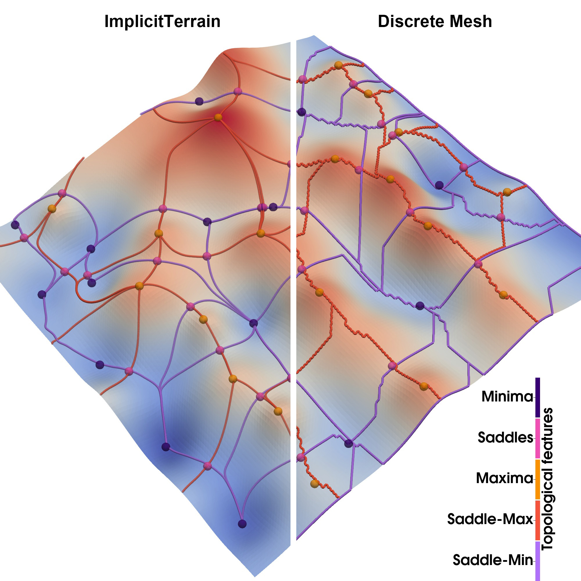
There is a need for a continuous surface model that can be used for topological analysis and is scalable to large-scale terrain data. Such accuracy of terrain surface and its high-order derivatives is pivotal for topological feature extraction and enhances many other analyses of terrain data, such as topography, hydrology, and geomorphology. In this paper, we propose a novel continuous surface modeling pipeline, ImplicitTerrain, that leverages the recent advances in the implicit neural representation (INR) to achieve a continuous surface model for terrain data analysis. For example, in Fig. 1, topological features extracted from ImplicitTerrain are well-aligned with the synthetic terrain surface. Benefiting from the interpolation capability, INR is a revolutionary representation that may achieve better memory efficiency than a discrete representation by decoupling the network size with the input data size.

However, there is still a gap between practical applications and the theoretical potential of INR. INR’s “over-smoothness” fitting result makes reconstructing the detailed surface geometry difficult, especially for high-resolution input [54]. Despite advancements (e.g., [62, 66]), for visual signals consisting of complex frequency components, obtaining accurate high-order derivatives is still challenging. The lengthy training process and the high computational cost of INR also limit its application in large-scale terrain data fitting and analysis. Besides, there is a domain difference between fitting the terrain height field and the photometric data, that the former requires both a plausible visual appearance and accurate surface restoration. Merging the gap between the theoretical potential and the practical applications of INR, ImplicitTerrain pioneers a feasible continuous terrain surface modeling pipeline that opens a new research avenue. Our main contributions are as follows:

• We introduce a novel Surface-plus-Geometry (SPG) cascaded INR model for high-resolution terrain surface modeling that keeps high reconstruction fidelity, reduces overall training time, and allows the topological analysis to be directly performed on the continuous manifold.

• We propose a progressive training strategy to train the SPG model from coarse to fine, significantly improving convergence speed while fulfilling the pre-processing requirement of topological and topographical analysis.

• Beyond surface fitting, we demonstrate the good alignment of the extracted topological features with the results based on the discrete Morse theory. Moreover, it shows superior perceptional and visual quality, reflecting terrain surfaces as perceived by human beings.

• Demonstrating ImplicitTerrain’s utility in calculations of various topographical features, i.e., slope, aspect, and curvature, directly from surface derivatives, underscoring its potential for comprehensive terrain data analysis.

2 Background and Related Work

2.1 Implicit neural representation

Different from the widely-known deep neural networks aiming to learn the hidden high-dimensional features such as semantic information of visual signal, INR is designed for reconstructing the input through neural network weights and it can be regarded as a revolutionary representation of the visual signals [71]. Most INRs are rooted in the Universal approximation theorem [35] - for a multi-layer perceptron (MLP) with a sufficient number of hidden units, any field function can be approximated within any precision [11]. For an MLP $\Psi\colon\mathbb{R}^{d}\to\mathbb{R}^{n}$ to reconstruct a visual signal, a common design of the network is to model a regression problem, in which the network takes individual coordinates $\vec{x}\in\mathbb{R}^{d}$ as input and predicts the field function values $\mathcal{F}|_{\vec{x}}\in\mathbb{R}^{n}$ corresponding to the coordinates, i.e., $\Psi(\vec{x})\approx\mathcal{F}|_{\vec{x}}$. Take a RGB image as an example, a neural work takes pixel coordinates $(u,v)\in\mathbb{R}^{2}$ and outputs pixel color $(r,g,b)\in\mathbb{R}^{3}$. This design of the network is also named as coordinate-based neural network. INR converts the signal to a continuous function representation defined on the input domain. Consequently, INR can be inferred in arbitrary resolutions and achieve better memory efficiency than a discrete representation by decoupling the network model size with the input data size [62]. The network can be stochastically optimized to be efficient and scalable to large input data [1]. Apart from the inherent continuity, INR is differentiable by an automatic differentiation technique that allows function gradient and higher-order derivatives to be easily accessible at any query location [62].

INR has gained much attention in various research fields where 2D images [10, 52, 40], 3D shapes [48, 30, 38, 72, 12, 68, 51, 1, 32], textures[56, 11, 49, 34], light fields [20, 5], dynamic fields [22, 36], and indoor and outdoor scenes [61, 47, 64, 70, 37, 39] are proposed to be converted into neural representations. For 3D objects, signed/unsigned distance functions [51, 13, 7, 75] and occupancy prediction networks [42, 53] are mostly used, while for 2D images, single MLP [62, 24] and decoder for feature grids [10, 46] are more common. Recently, researchers have shown the representation power of INR in biomedical data [74, 45], satellite images [20, 64, 70], and physics-informed simulations [16, 14]. Others take advantage of INR’s compression capabilities in image [63, 74, 6, 23] and video compression [8, 9].

Through Fourier analysis, many neural networks, such as ReLU MLP, suffer from capturing high-frequency components of the input signals, because their fitting power biases toward the low-frequency components, known as spectral bias [54, 4, 77]. It leads to the “over-smoothness” issue. FFN [66] makes use of Neural Tangent Kernel (NTK) techniques to analyze this phenomenon and proposes to use positional encoding techniques to counter the spectral biases and capture more high-frequency details. Another well-known approach is SIREN [62], which makes use of the sinusoidal non-linear activation function with carefully designed network initialization. A SIREN model can be expressed as

$$\Psi(\vec{x}) =\Omega_{n}(\psi_{n-1}\circ\psi_{n-2}\circ\cdots\circ\psi_{0})(\vec{x})+\vec{b}_{n}$$ (1)

$$\psi_{i}(\vec{x}) =\sin(\Omega_{i}\vec{x}+\vec{b}_{i})$$ (2)

where $\psi_{i}$ is the $i$-th layer of the MLP and $(\Omega_{i},\vec{b}_{i})$ is the corresponding network weights and biases. This design choice allows the model to be written in a composition of sinusoidal functions and the derivatives of the network have similar expressions such that the training process is not only targeting the field function $\mathcal{F}$ but also its derivatives $\{\nabla_{\vec{x}}\mathcal{F},\nabla_{\vec{x}}^{2}\mathcal{F},\ldots\}$ [62]. This design is important for topological analysis and topographical feature calculation since the reconstructed surface function is smooth and an accurate gradient field is necessary. ImplicitTerrain takes advantage of the compactness and the representation power of INR which may achieve better accuracy with less computational resources. As shown in this paper, ImplicitTerrain demonstrates the effectiveness and implementation simplicity in the field of terrain data analysis.

2.2 Topology-based terrain analysis

Morse theory. Morse theory captures the relationships between the topology of a manifold and the critical points of a function defined on it [43]. For a smooth scalar function $f$ on domain $D\subseteq\mathbb{R}^{2}$, critical points of $f$ are those gradients of $f$ vanishes. The index $k_{p}$ of a critical point $p$ is the number of negative eigenvalues of the Hessian matrix $\mathcal{H}|_{p}$ of the second-order partial derivatives of $f$ at $p$. If $k_{p}=0$, $p$ is a minimum, $k_{p}=1$ a saddle, and $k_{p}=2$ a maximum. A smooth function $f$ is a Morse function if every critical point $p$ is non-degenerate, i.e., $\mathcal{H}|_{p}(f)\neq 0$.

An integral line of $f$ is a path tangent to gradient $\nabla f$, tracing the steepest ascent or descent from one critical point to another. An integral line connecting two critical points of consecutive index is called a separatrix line. Given a critical point $p$ of index $k$, the integral lines converging at $p$ of index $k_{p}$ form a $k$-cell, called the descending $k$-manifold of $p$. Dually, integral lines originating at $p$ form a ($d$-$k$)-cell, called the ascending $k$-manifold of $p$. The ascending manifolds partition $D$ into cells forming the ascending Morse complex and descending Morse complex, respectively.

A Morse function $f$ is a Morse-Smale function when the ascending and descending manifolds intersect transversally. Cells obtained as the intersection of descending and ascending 2-manifolds of a Morse-Smale function $f$ decompose $D$ into a Morse-Smale complex. A critical net is the 1-skeleton of the Morse-Smale complex, which consists of the critical points and the separatrix lines connecting them.

The combinatorial structure of the critical net is described by the Morse Incidence Graph (MIG) [15]. The nodes of the MIG correspond to the critical points of $f$, while its arcs correspond to the separatrix lines, i.e., the connections between pairs of critical points. A value is associated with each arc of the graph, which is the absolute value of the difference between the function value at the critical points corresponding to its extreme nodes, called persistence. Insignificant critical points that do not contribute to the main topological structure of a surface are usually removed by the MIG based on the persistence values. The two fundamental operators for simplifying a MIG, while maintaining its topological integrity are: Minimum-Saddle-Minimum, which collapses two minima adjacent to the same saddle into one of them, eliminating also the common saddle, and its dual Maximum-Saddle-Maximum, which is defined symmetrically [18].

Discrete approaches. A variety of methods have been proposed in the literature to identify critical points and trace separatrix lines in the discrete case when a terrain is defined by a set of points either at the vertices of a regular square grid (gridded data), or scattered in the plane. In the case of gridded data, earlier approaches interpolate the data through smooth functions, including a $C1$-differentiable Bernstein-Bezier bi-cubic function [2], as well as bilinear $C0$-interpolant and bi-quadratic interpolant [58, 57], with derivatives computed numerically in [2] and analytically in [58, 57]. The efficacy of these methods depends on precise tuning of the approximation functions to avoid false critical points and maintain domain-wide continuity.

Smooth interpolation methods also struggle with scalability, especially with large terrain datasets. Thus, discrete methods based on triangulating the data points have been most widely used, for instance, in Topology ToolKit (TTK) [67], a popular topological data analysis toolkit.

Two discrete approaches have been applied to triangulated terrains, namely piecewise-linear Morse theory by Banchoff [3] and discrete Morse theory by Forman [28]. The former identifies and classifies critical points per [3] for polyhedral surfaces, tracing separatrix lines from saddles to minima and maxima along triangle edges.

Discrete Morse theory on a triangle mesh is based on extending the elevation function from the vertices to the edges and triangles of the mesh and on defining a discrete gradient field, usually called a Forman gradient. Several algorithms have been developed to compute a Forman gradient, its critical features [33, 55, 60] and simplicial complexes [69, 25]. The Forman gradient is the basis for an efficient computation of discrete separatrix lines through mesh traversals. See the supplementary materials for discrete Morse theory details and [18] for a comprehensive review.

The Forman method is favored in terrain analysis for its derivative-free nature, offering efficiency and scalability for large datasets [26, 27]. Yet, its topological accuracy can depend on mesh construction choices, like diagonal selection in grid triangulation [18].

3 Methodology

ImplicitTerrain represents the terrain surface function $\mathcal{F}_{s}$ via coordinate-based neural networks that are trained progressively from the ground elevation data $I\in\mathbb{R}^{H\times W}$ in GeoTIFF [41] format. The pipeline of ImplicitTerrain, as shown in Fig. 2, consists of three main stages: (I) Sec. 3.1 Input raster data preprocessing, (II) Sec. 3.2 Surface-plus-Geometry (SPG) model fitting, which consists of two cascaded networks: surface model $\Psi_{s}$ and geometric compensation model $\Psi_{g}$, and (III) Sec. 3.3 Topological feature extraction and Sec. 4.6 topographical feature computation.

Figure 2: The pipeline of the ImplicitTerrain. Firstly, terrain data is preprocessed as a Gaussian pyramid for progressive fitting. Then, the cascaded Surface-plus-Geometry (SPG) model is trained to fit the smoothed terrain surface and the residual/displacement map in order. Finally, various terrain data analyses are supported by the smooth surface model. Model weights can be serialized for storage and inference to reconstruct the terrain surface with flexible structures (grids or TINs) and resolutions. Better viewed in the digital version.

3.1 Input raster data preprocessing

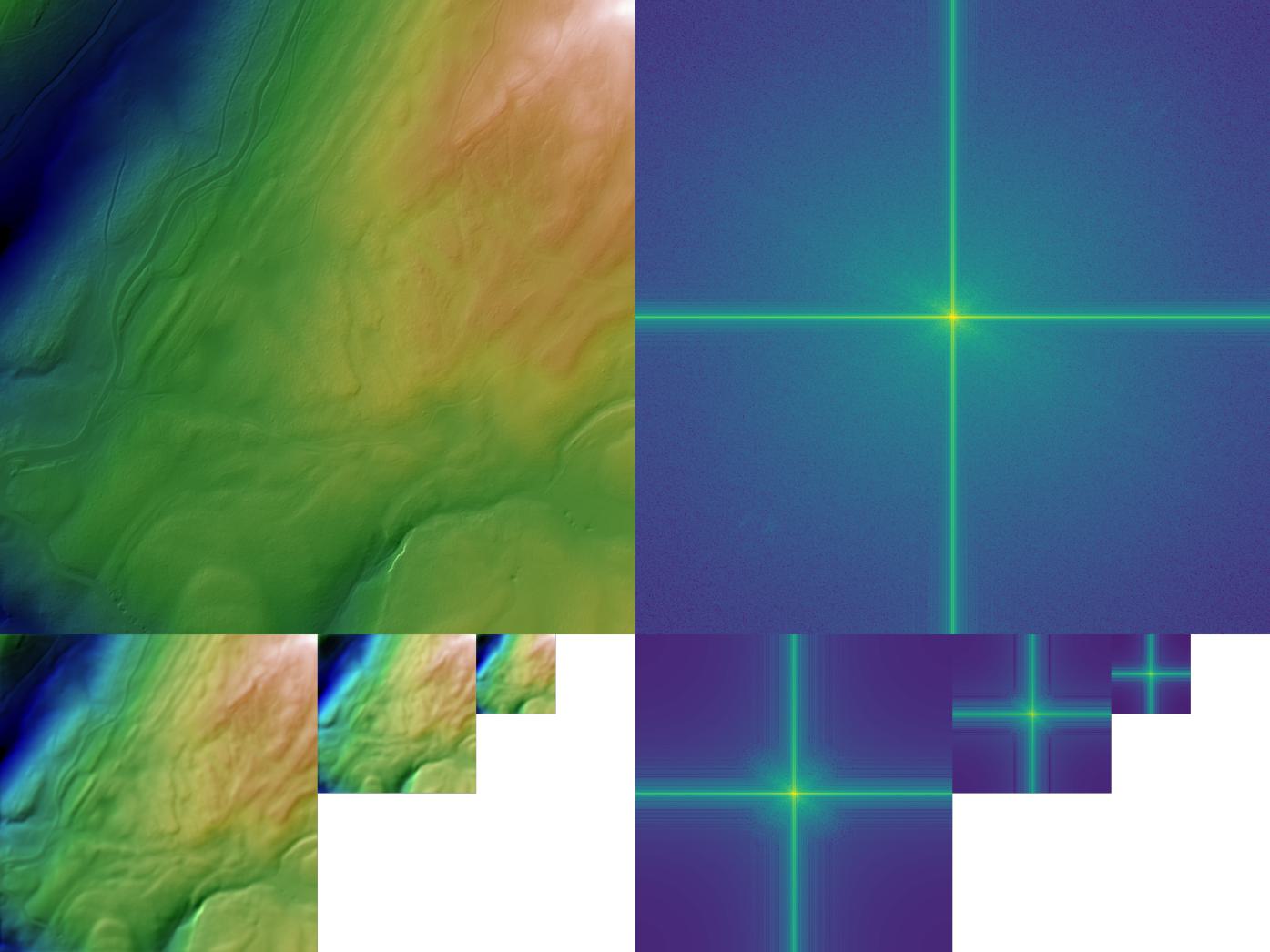
As a common practice in terrain data analysis, a smoothing process is applied to remove the noise and artifacts during the data acquisition process. This process may diminish the visual quality of the terrain surface since the high-frequency details are absent. To keep the high fidelity of the input signal, we make use of a low-pass Gaussian filter iteratively to construct a multi-resolution Gaussian pyramid of the input raster data as shown in Fig. 2, where the bottom layer is the original input $I$ and the layer on top is the smoothed version of the previous layer with half the size. This multi-resolution pyramid allows the progressive training of $\Psi_{s}$ from top to bottom (except the bottom layer) as detailed in Sec. 3.2. As shown in Fig. 3, surface details are preserved only in the bottom layer that is used by $\Psi_{g}$.

Figure 3: Gaussian pyramid and frequency view of $\text{Swiss}_{1}$ dataset.

3.2 Surface-plus-Geometry (SPG) model fitting

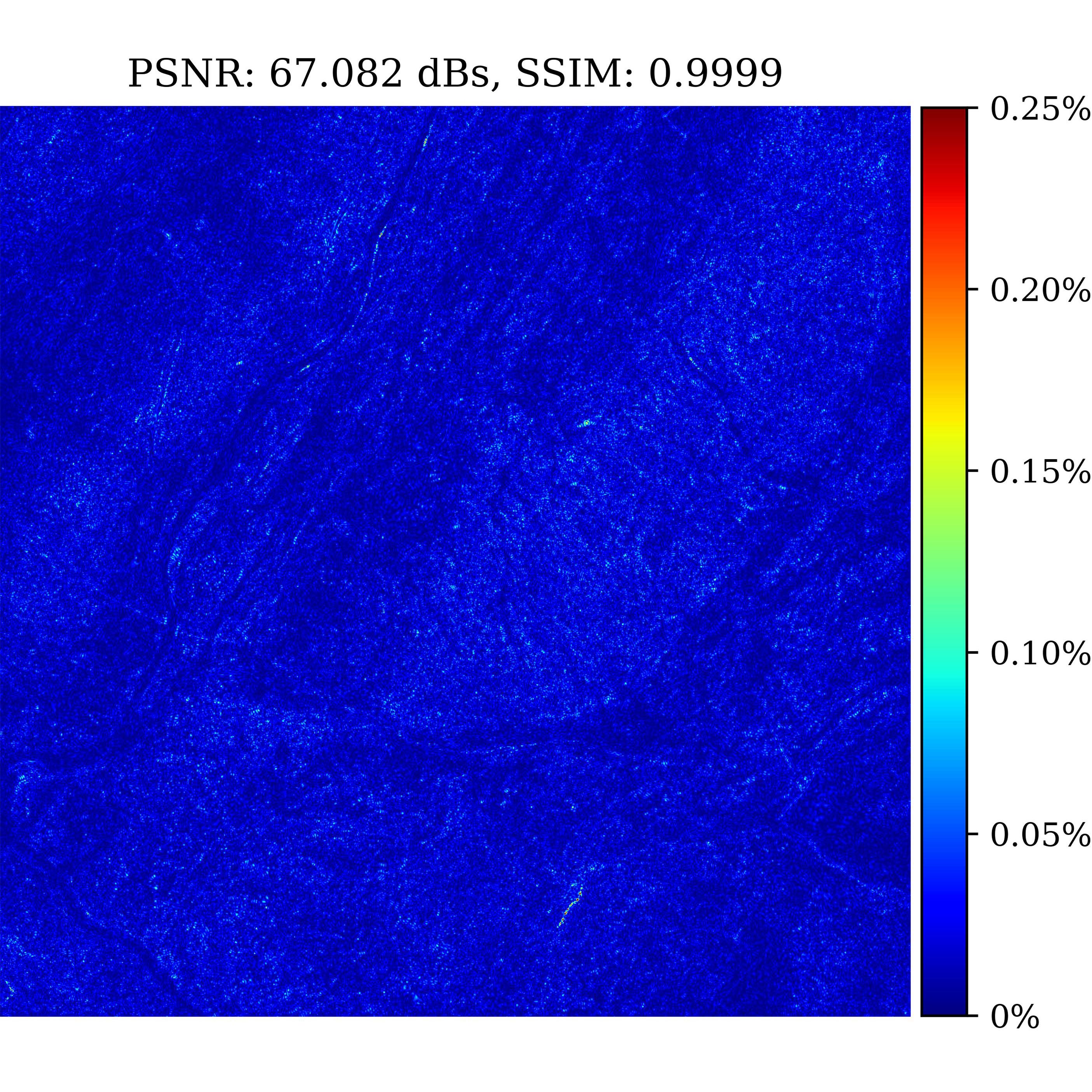
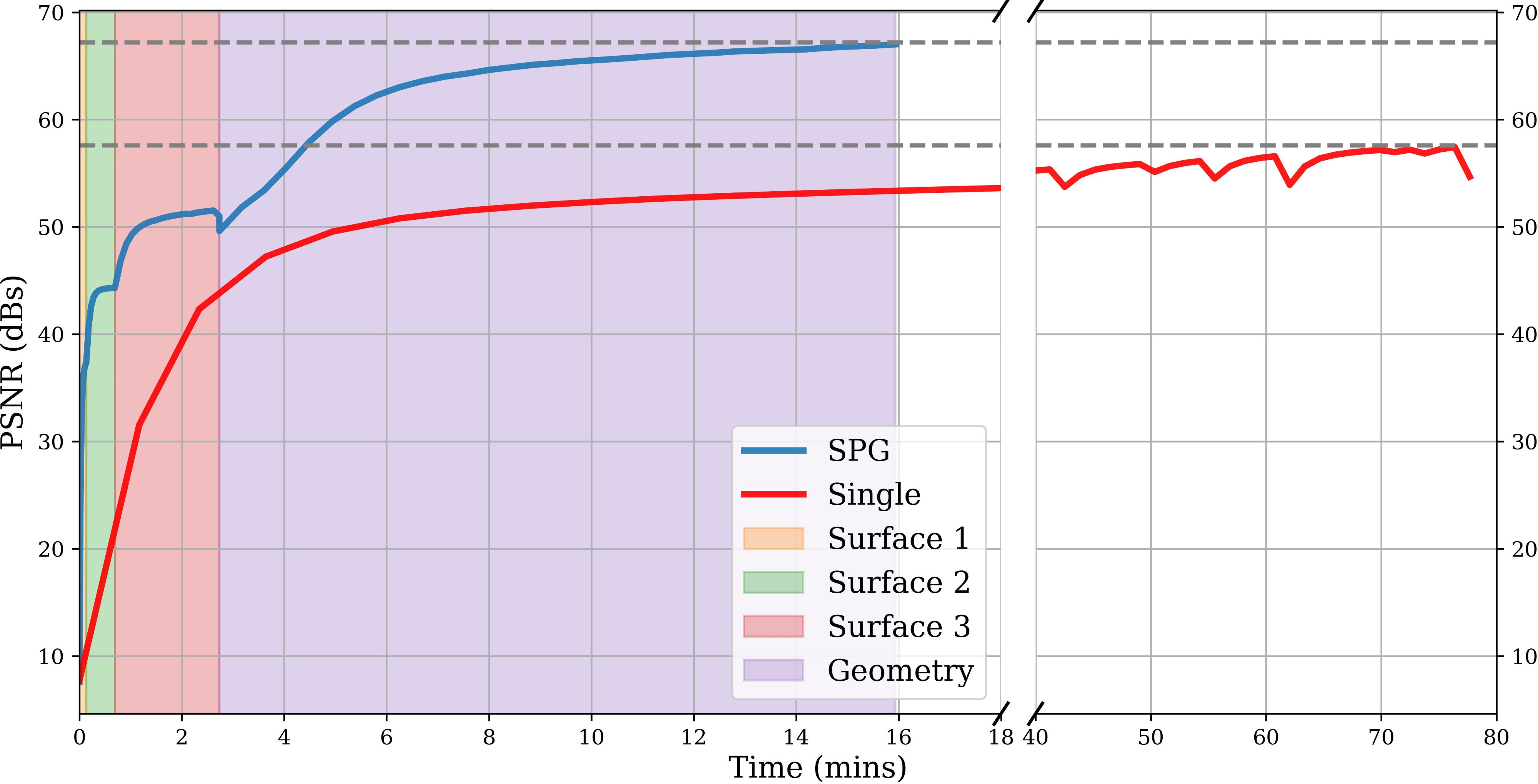
An MLP with sinusoidal non-linear activation function as in SIREN [62] is used for both $\Psi_{s}$ and $\Psi_{g}$ for simplicity and efficiency. This architecture allows accurate fitting of both $\mathcal{F}_{s}$ and its derivatives $\{\nabla_{\vec{x}}\mathcal{F}_{s},\nabla_{\vec{x}}^{2}\mathcal{F}_{s},\ldots\}$. $\Psi_{s}$ and $\Psi_{g}$ can be evaluated at arbitrary query coordinates and derivatives are calculated by the automatic differentiation. The network configuration can be determined heuristically to trade-off between model size and fitting accuracy. However, with the increment of the model size, the training time also increases, especially when $I$ is of high-resolution. Inspired by the spectral bias, we separate the hard-to-fit high-frequency components from $I$ by the Gaussian pyramid in Sec. 3.1 and fit $\Psi_{s}$ progressively from top to bottom to reduce the convergence time and smooth the training process. With less computational cost, $\Psi_{s}$ converges faster to the smoothed terrain surface. Then, $\Psi_{g}$ fits the absent details from $\Psi_{s}$ via the residual learning, as shown in Fig. 2. The residual is the pixel-wise difference between the high-resolution inference of $\Psi_{s}$ and the original input $I$. Fitting the residual shares similar intuition as the displacement map in computer graphics rendering and in the work by Wang et al. [76]. Therefore, $\Psi_{s}$ represents a smooth surface function with a stable gradient field, benefitting the following topological analysis in Sec. 3.3. Compensating $\Psi_{s}$ with surface details in $\Psi_{g}$ via the addition of both models’ output, the reconstructed surface function $\hat{\mathcal{F}_{s}}$ is more accurate and visually plausible than a single model design. As we will show in the ablation study Sec. 4.4, the SPG model achieves better overall fitting accuracy (PSNR 67.08 dBs vs. 57.66 dBs) and faster convergence speed ($\approx$ 4 times) than a single MLP model with approximately the same number of parameters.

3.3 Topological feature extraction

Surface model $\Psi_{s}$ can be used as a smooth surface function allowing the direct inference of height values and derivatives at any query locations within the domain. This characteristic greatly simplifies the algorithm design to identify critical points and build the connection between them. Without hindrance, Morse theory can be directly applied to the smooth function $\Psi_{s}$, avoiding the difficulties of approximating the gradient field on discrete meshes.

Identify critical points. Critical points are the points where the gradient vanishes (i.e., $||\nabla\mathcal{F}_{s}||=0$). For terrain surface, critical points can be classified into three types: Maximum, Minimum, and Saddle. According to Sylvester’s criterion [31], this classification can be achieved by the second-order derivatives, i.e., Hessian matrix $\mathcal{H}|_{\vec{p}}\in\mathbb{R}^{2\times 2}$ at the critical point coordinate $\vec{p}$. To locate the critical points, we trace the zero-cross points of the gradient field by a simple gradient descent algorithm to minimize the gradient norm $||\nabla\Psi_{s}||$. Candidate critical point locations are determined by considering the value differences of the neighboring vertices to the center vertex on smoothed meshes. Clone and random jitter of the coordinates are applied to these candidate coordinates. For each step, the gradient norm $||\nabla\Psi_{s}||$ minimization direction $\vec{d}$ takes the form:

$$\begin{split}\vec{d}=&-\left\langle\partial||\nabla\Psi_{s}||/\partial x,\partial||\nabla\Psi_{s}||/\partial y\right\rangle\\ =&-\left\langle f_{x}f_{xx}+f_{y}f_{yx},f_{x}f_{xy}+f_{y}f_{yy}\right\rangle\end{split}$$ (3)

where $f_{x},f_{y}$ are the first-order derivatives of $\Psi_{s}$ and $f_{xx},f_{xy},f_{yx},f_{yy}$ are the second-order derivatives.

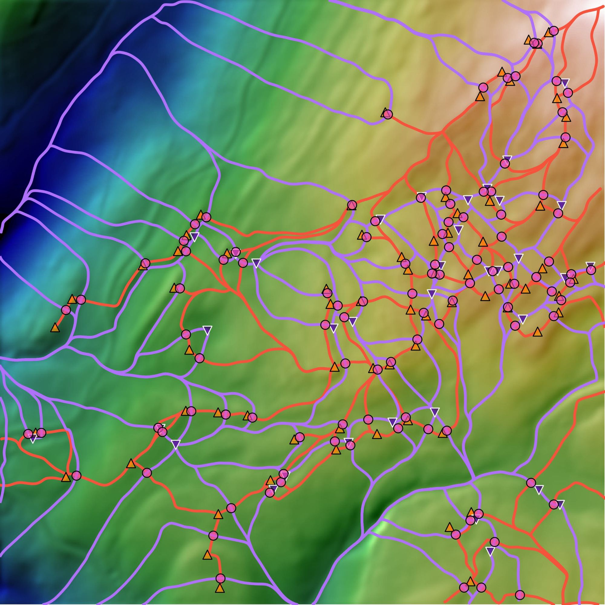
Separatrix lines and MIG. As detailed in Sec. 2.2, separatrix lines are a subset of integral lines that connect the critical points, depicting the topological skeleton of the terrain surface. For each Saddle, the separatrix lines connect it to two neighboring Minimum and two Maximum points. The eigenvector of the Hessian matrix $\mathcal{H}$ at the Saddle point is used to determine the starting directions of the four separatrix lines. Heading to the Maxima/Minima, the gradient field is traced to maximize/minimize the height values. Determining the relationship between the critical points helps to build the MIG of full resolution, from which, through persistence-based simplification, the prominent topological structure of the terrain surface is extracted as in Fig. 2. The design and implementation details of the tracing algorithms are provided in the supplementary material.

4 Experiments

We evaluate the performance of ImplicitTerrain on terrain dataset from two aspects: model accuracy and topological analysis results. We employ an open-source library to compute the separatrix lines and simplified MIGs by computing Forman gradients. In the rest of this paper, we refer to this library as the Forman method. Due to the lack of ground truth topology of the real-world terrain, in Sec. 4.2, a synthetic terrain model is generated to demonstrate the effective alignment between results from ImplicitTerrain and Forman method. In Sec. 4.3, high-resolution terrain data is fed to the pipeline. In Sec. 4.4, we design an ablation experiment to show the effectiveness and efficiency of our SPG model in terms of training time and fitting results. In Sec. 4.5, we conduct experiments for the noise robustness of the surface topology obtained from our surface model.

4.1 Experiment setup and evaluation metrics

Both $\Psi_{s}$ and $\Psi_{g}$ use an MLP with 3 hidden layers and 256 hidden units per layer to fit an input 1000$\times$1000 raster data $I$ for the height field of $1\text{km}^{2}$ terrain surface. Height values and the coordinates are normalized into the $[-1,1]$ range. The sinusoidal activation function and the same weight initialization are applied as in SIREN [62]. As in Fig. 2, $\Psi_{s}$ is progressively fitted on the top 3 layers of a 4-layer Gaussian pyramid constructed with a Gaussian kernel size $\sigma=4.0$. The final optimization target $I_{s}$ of $\Psi_{s}$ is of size 500$\times$500. Then, $\Psi_{g}$ fits the residual between $I$ and the surface model’s inference output $I_{\Psi}$. Both models are trained for 3000 steps with the Adam optimizer with a learning rate of 1e-4. All the experiments are conducted on a computation node with a 24-core CPU (AMD EPYC 7352) and an NVIDIA A5000 GPU. From the aspects of model accuracy and topological analysis results, various evaluation metrics are used to measure the performance of the ImplicitTerrain.

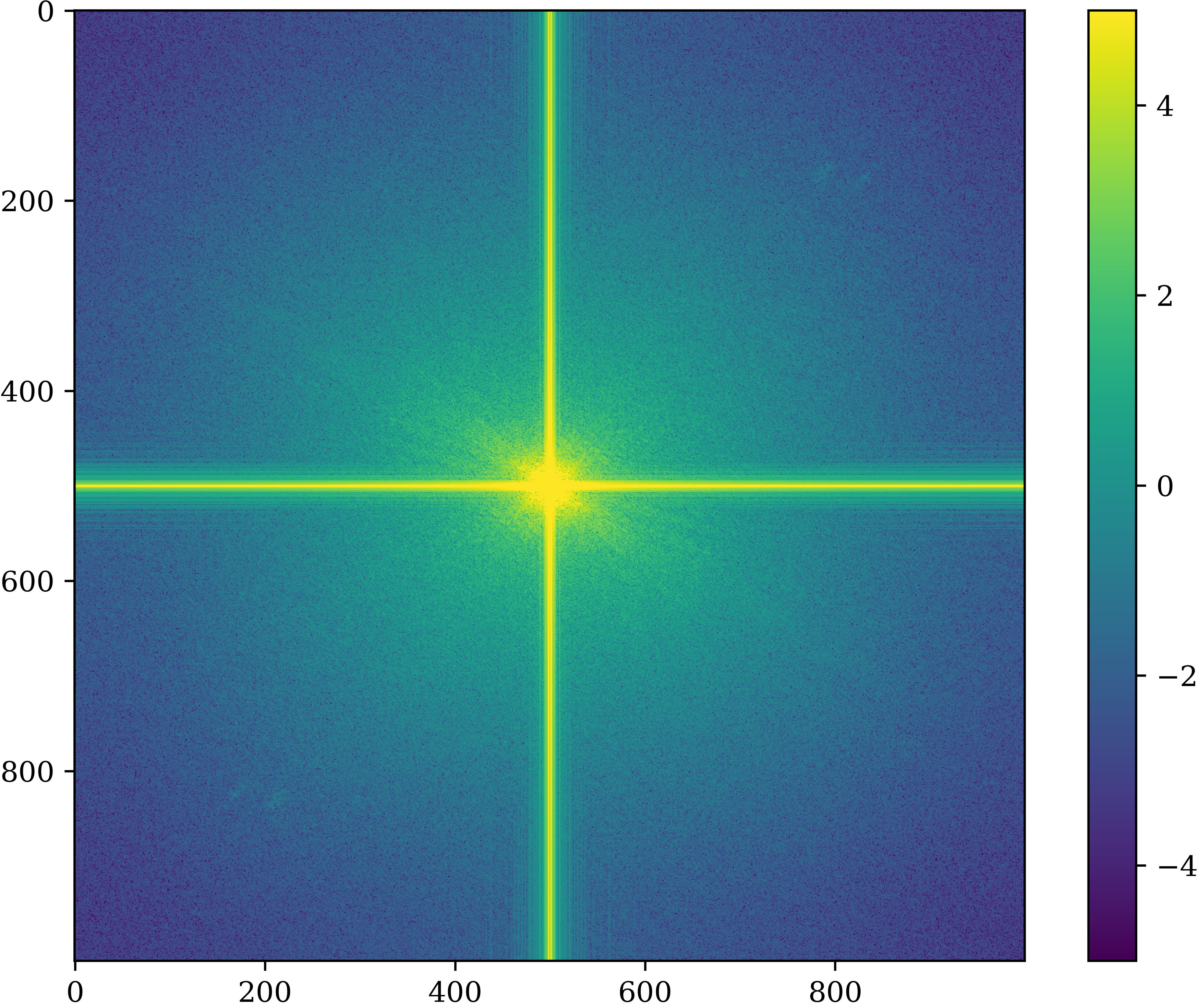
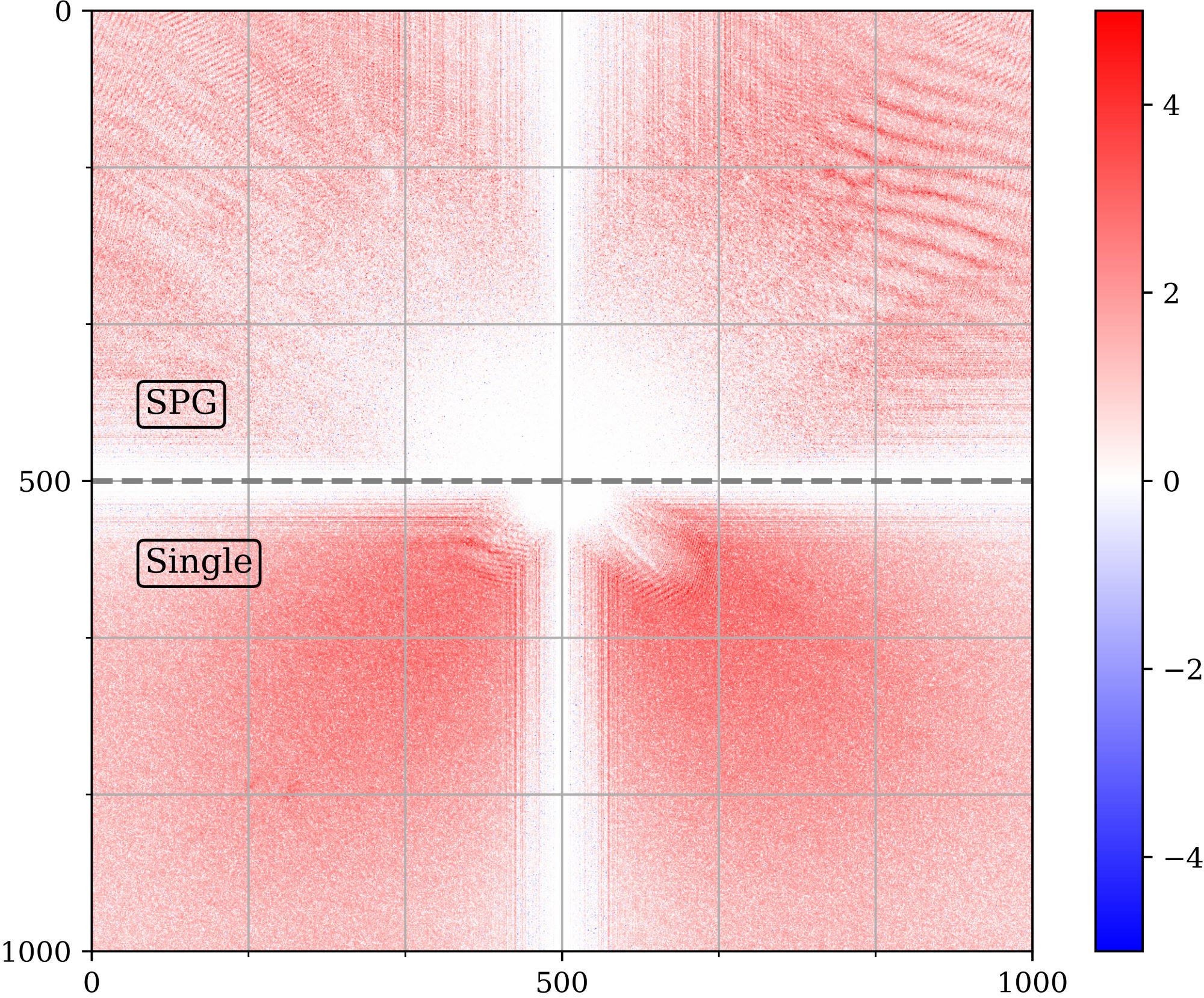
Model accuracy. To measure the reconstruction accuracy of the ImplicitTerrain, peak signal-to-noise ratio (PSNR) and structural similarity index measure (SSIM) are calculated. For PSNR calculation, since there is no boundary for the height field, the maximum possible value of the signal is set to $1.0$. SSIM metric evaluates the visual similarity between the model output and the original input data. For evaluating the surface model $\Psi_{s}$, the frequency band reconstruction capability is calculated by the difference between the log-scaled magnitude of the Fourier transform of $I_{s}$ and $\Psi_{s}$’s inference result in $I_{\Psi}$, i.e. $\log(|I_{s}|)-\log(|I_{\Psi}|)$. Since the gradient field is important for topological and topographical analysis, we measure the gradient field reconstruction accuracy in terms of the pixel-wise difference of gradient norm and direction between our model’s estimations $\nabla\Psi_{s}$ and the results derived from $I_{s}$ by pixel shifting.

Topological analysis. To evaluate the topological analysis result of $\Psi_{s}$, we measure the degree of alignment between the topology of our surface model and the topology from Forman method. The MIGs from both methods are simplified by a persistence value of 1 meter which is heuristically set to keep prominent critical points from Forman method. The MIG alignment is measured from two aspects: (1) critical points matching as a binary classification method, and (2) MIG-based persistence diagram. Critical points are matched based on spatial closeness and the result is reported in Precision, Recall, and $F_{0.5}$ score, which regards the precision as twice as important as the recall rate. To highlight the topological features in the MIG, we make use of its persistence diagram, which is a visualization of connected critical point pairs [29]. It depicts the evolution of the terrain surface topology and highlights the critical points representing prominent topological features, e.g., mountain peaks. We use the Wasserstein distance ($WS$) to measure the similarity between two persistence diagrams, which is defined as the minimal distance achieved by a perfect matching of two diagrams. A smaller $WS$ value indicates a higher similarity between two persistence diagrams.

For the Forman method applied to the regular gridded mesh, it is known that the mesh configuration (connectivity between neighboring vertices in a diagonal direction) may influence the MIG result [18]. Satisfying the Delaunay triangluation [19] of the gridded data, we consider two different mesh configurations for the Forman method: each vertice is connected to its (N, S, E, W, NW, SE) or (N, S, E, W, NE, SW) neighbors, named as Mesh1 and Mesh2 respectively. Considering the missing ground-truth persistence diagram and the influence of mesh configuration on the MIG, we further propose to evaluate the MIGs by the ratio of Wasserstein distance as

$$WS_{ratio}=\frac{\min(WS(\Psi_{s},\text{Mesh1}),WS(\Psi_{s},\text{Mesh2}))}{WS(\text{Mesh1},\text{Mesh2})}$$ (4)

If this ratio value is between 0 and 1, it means that the MIG from $\Psi_{s}$ is closer to the Forman method result than the distance between the MIGs of Mesh1 and Mesh2. Thus, we consider the topology obtained from our method to be accurate. Limited by the paper length, details about the Wasserstein distance calculation and the influence of mesh configuration are provided in the supplementary materials.

4.2 Synthetic terrain data

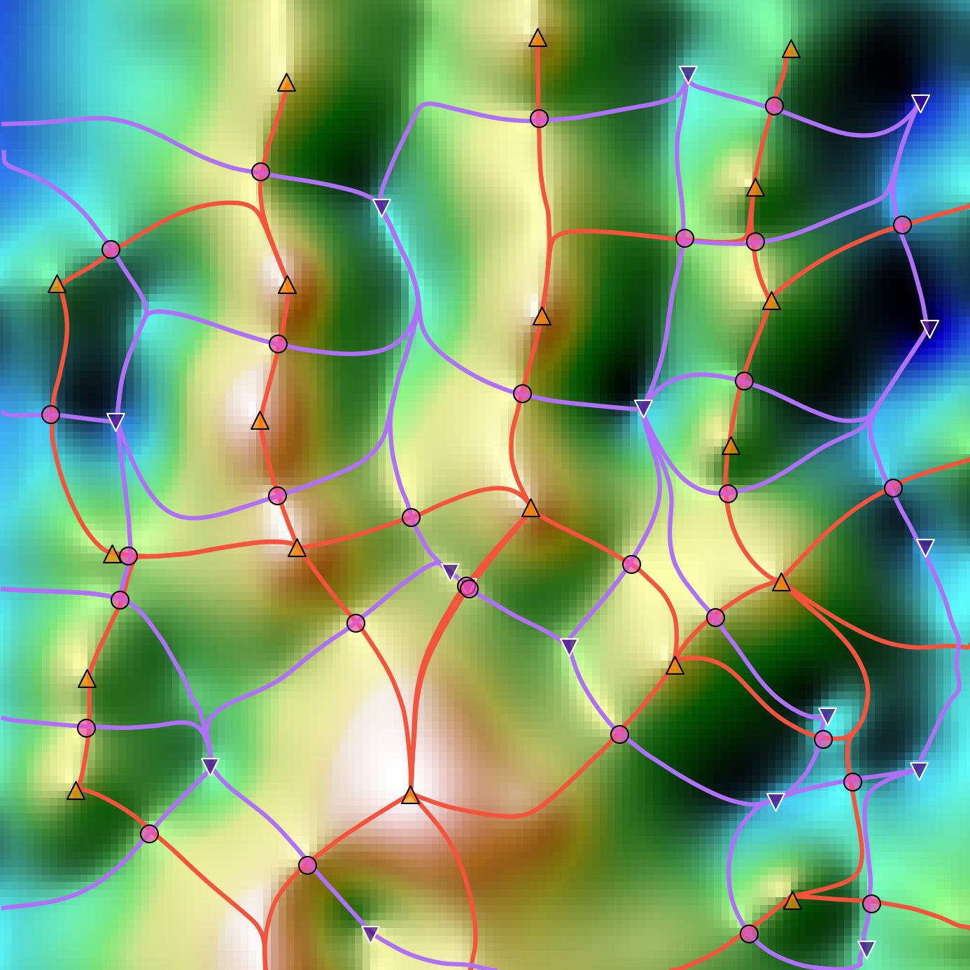
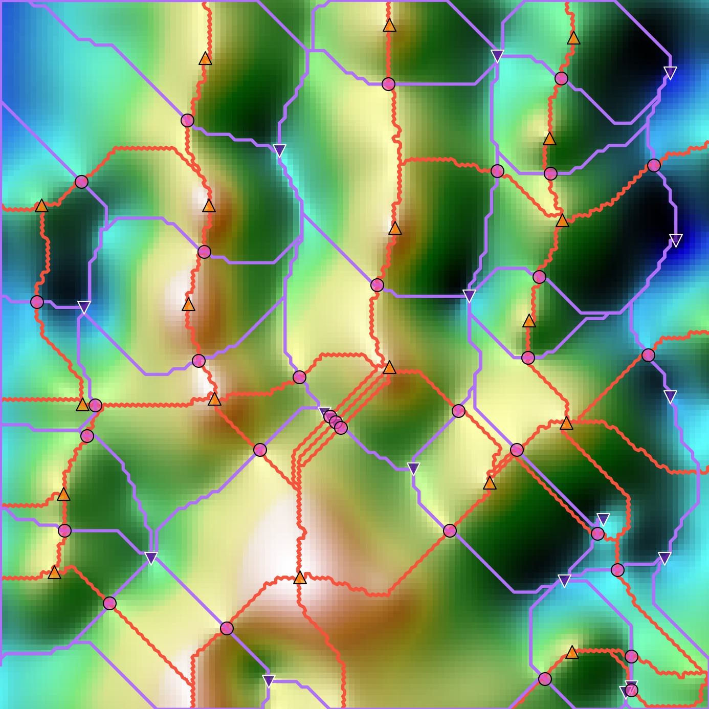
Before evaluating the ImplicitTerrain on real-world terrain data, synthetic terrain data with simple topology is generated to show the effective alignment of our surface model analysis results to the Forman method results. The synthetic terrain is of side length 256 with height values between $[0,200]$ and is generated as a combination of 2D random Gaussian signals with various covariances as shown in Fig. 1. Particularly, knowing the surface gradient of the synthetic terrain allows a better data triangulation than the Mesh1 and Mesh2. The triangulation of each grid cell is determined by the surface gradient, leading to visually better separatrix lines by Forman method. Due to the simplicity of this dataset, our models are also shrunk to have 3 hidden layers and 128 hidden units. As shown in Fig. 4, the critical points, separatrix lines, and MIGs from both methods form a good visual alignment. Quantitative evaluations of the topological analysis results are shown in Tab. 1. $F_{0.5}$-score value is $1.0$ and the small $WS_{ratio}$ proof the high similarity between our results and Forman method. Besides the correctness of the topological analysis results, it is obvious that the smooth (zigzag free) separatrix lines obtained from the ImplicitTerrain are visually plausible and faithfully align with the terrain surface. These smooth and accurate separatrix lines might lead to better segmentation results based on the Morse-Smale Complexes.

Name	precision	recall	$F_{0.5}$ score	$WS_{ratio}$
$\text{Synth}_{ours}$	1.00	1.00	1.00	0.68
$\text{Swiss}_{1}$	0.90	0.96	0.91	0.17
$\text{Swiss}_{2}$	0.91	0.831	0.89	0.31
$\text{Swiss}_{3}$	0.89	0.78	0.87	0.69
$\text{Swiss}_{4}$	0.91	0.83	0.89	0.35

Table 1: Topological analysis results of the synthetic and real-world terrain. $WS_{ratio}$ between $[0,1]$ indicates the MIGs from both methods are well aligned.

(a) Separatrix lines - ImplicitTerrain.

(b) Separatrix lines - Forman method.

(c) MIG - ImplicitTerrain.

(d) MIG - Forman method.

Figure 4: Comparison of topological analysis results of the synthetic terrain. Node colors and shapes represent the critical point types and the edge colors represent the separatrix lines as in the legend of (c) and (d). Better viewed in the digital version.

4.3 Real-world terrain data

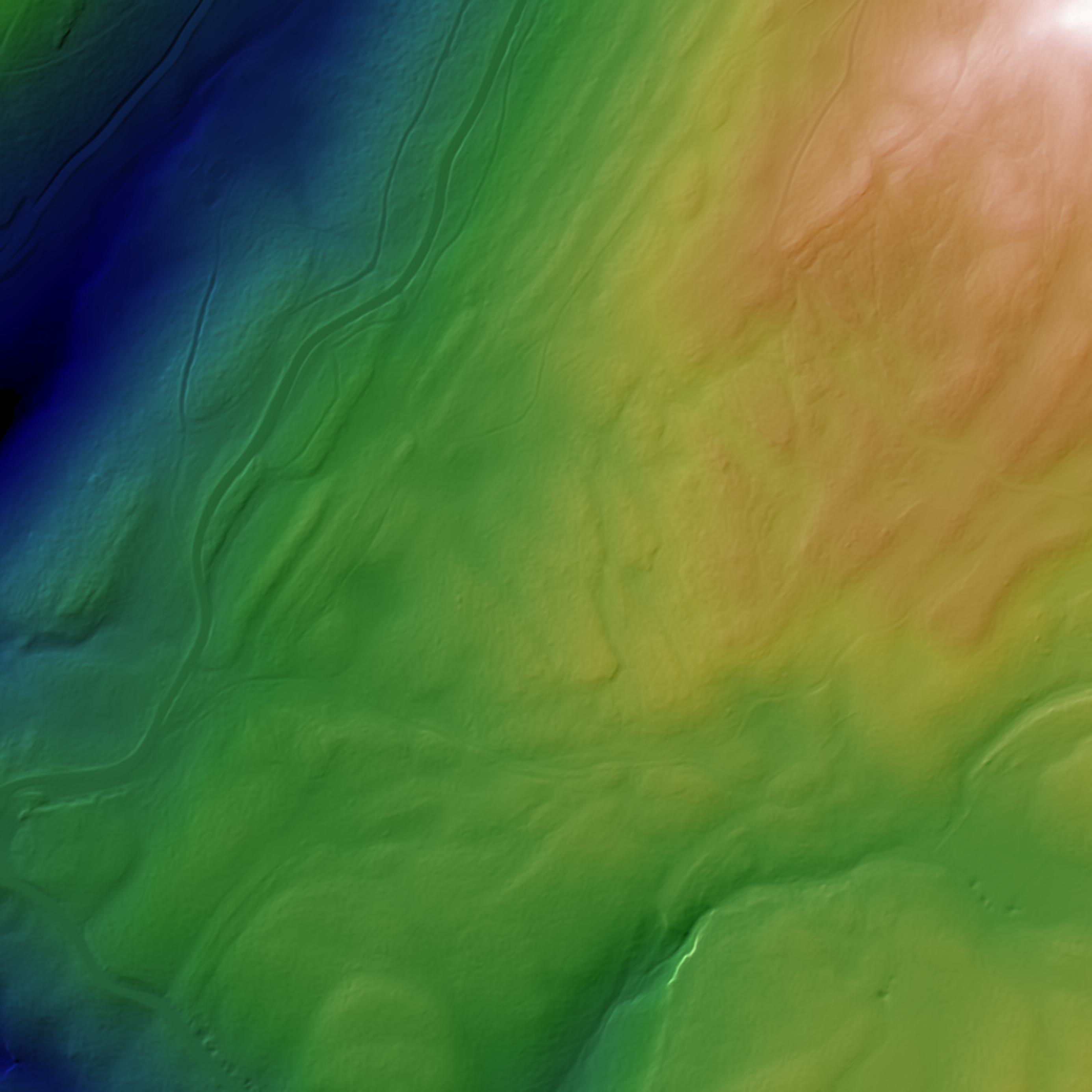
Swisstopo dataset swissALTI3D [65] provides high-resolution digital elevation information of the Switzerland terrain surface without vegetation. Four different tiles $\text{Swiss}_{k}$ ($k\in\{1,2,3,4\}$) of size 1km$\times$1km are selected with various terrain characteristics as input data and each tile is of resolution 1 meter per pixel. Limited by the paper length, we only put the results for $\text{Swiss}_{1}$ tile and the rest results with extra analysis can be found in the supplementary materials. As shown in Tab. 2, ImplicitTerrain model size is 80% less than the input raster file and the surface fitting criteria all show our method provides a very good reconstruction of the terrain surface function. The gradient field, especially the gradient direction, is accurately reconstructed, benefitting the following topological analysis and topographical calculation. Besides, in Fig. 5, the detailed textures over the terrain surface are preserved. With the accurate fitting of the terrain gradient field, in Tab. 1, the results of critical point matching and Wasserstein distance ratio show that our surface model is able to correctly capture the topological features from the input terrain. The value of the Wasserstein distance ratio is small enough to confirm that our persistence diagram is closely aligned with the Forman method result. As shown in Fig. 5, separatrix lines and critical points together delineate the terrain topology. Ridges/valleys between the mountain saddles and the peaks/basins are accurately depicted in the plot.

Name	Sizes (MBs)	Size ratio	$\Psi_{s}$ PSNR	$\Psi_{s}$ SSIM	Freq diff $\times 10$	Grad norm diff $\times 10$	Grad direction diff (rad) $\times 10$	SPG PSNR	SPG SSIM
$\text{Swiss}_{1}$	$1.51/7.6$	0.20	64.85	0.9999	1.49$\pm$2.31	0.54$\pm$0.52	0.62$\pm$1.10	67.08	0.9999
$\text{Swiss}_{2}$	$1.51/7.6$	0.20	60.53	0.9998	0.95$\pm$2.08	0.77$\pm$1.00	0.61$\pm$0.77	52.34	0.9992
$\text{Swiss}_{3}$	$1.51/7.6$	0.20	59.75	0.9998	0.13$\pm$0.29	0.86$\pm$1.05	0.72$\pm$1.02	58.93	0.9997
$\text{Swiss}_{3}$	$1.51/7.6$	0.20	62.54	0.9999	0.17$\pm$0.32	0.56$\pm$0.61	0.46$\pm$0.57	66.59	0.9999

Table 2: Numerical evaluation of the fitting results of the real-world terrain. Sizes are the total model sizes and the input raster size, and Size ratio is their ratio. $\Psi_{s}$ PSNR and $\Psi_{s}$ SSIM are the fitting accuracy of the surface model to the smoothed data. SPG PSNR and SPG SSIM are the fitting accuracy of the SPG model to the original input. For the surface model, Freq diff is the mean and standard deviation of the frequency domain difference. Grad norm/direction diffs are the mean and standard deviation of the difference of gradient norm and direction between $\nabla\Psi_{s}$ and the estimated image gradient from $I_{s}$. $\times 10$ denotes the scaling factor for better numerical representation.

(a) Hillshade of SPG output.

(b) Absolute error of the fitting.

(c) Separatrix lines.

(d) MIG.

Figure 5: ImplicitTerrain fitting results and topological features extracted from $\text{Swiss}_{1}$. (b) shows the fitting error with red color mapping to 0.25% error. Better viewed in the digital version.

4.4 Ablation study: SPG model vs. single model

To counter the harm of spectral bias, we propose this simple-but-effective SPG pipeline which takes advantage of the downstream task requirement - it is a common practice to smooth the terrain surface before topological and topographical analysis, especially for high-resolution inputs. Our SPG model preserves a detailed visual quality of the terrain surface texture while effectively capturing topological features as in Fig. 5. To further show this design’s benefit to fitting accuracy and training time, we compare it to a single model with about the same number of trainable parameters - 3 hidden layers with 512 hidden units. In Fig. 6, we plot the smoothed (via Exponential Moving Average) PSNR values averaged for 5 rounds, with reference to the training time. Same as in the pipeline, both models are fitted for 6000 steps in total. Our progressively fitting model converges much faster and more accurately than the single model which takes 4 times more time to achieve a worse fitting accuracy (PSNR 67 dBs vs. 58 dBs). Additionally, by analyzing the frequency domain difference, Figure 7 shows that the design of SPG helps increase the fitting capacity of the network, explaining the better PSNR value it achieves.

Figure 6: Ablation comparison of the fitting accuracy between SPG and single model w.r.t. training time. Colored regions denote different training stages of the SPG model.

(a) Fourier transform of the $\text{Swiss}_{1}$.

(b) Frequency domain loss.

Figure 7: Freqency domain comparison of the fitting results. (a) shows the ground truth. (b) Since the Fourier transform result is central symmetric, SPG and single model frequency domain loss are plotted together as labeled in the figure.

4.5 Noise robustness

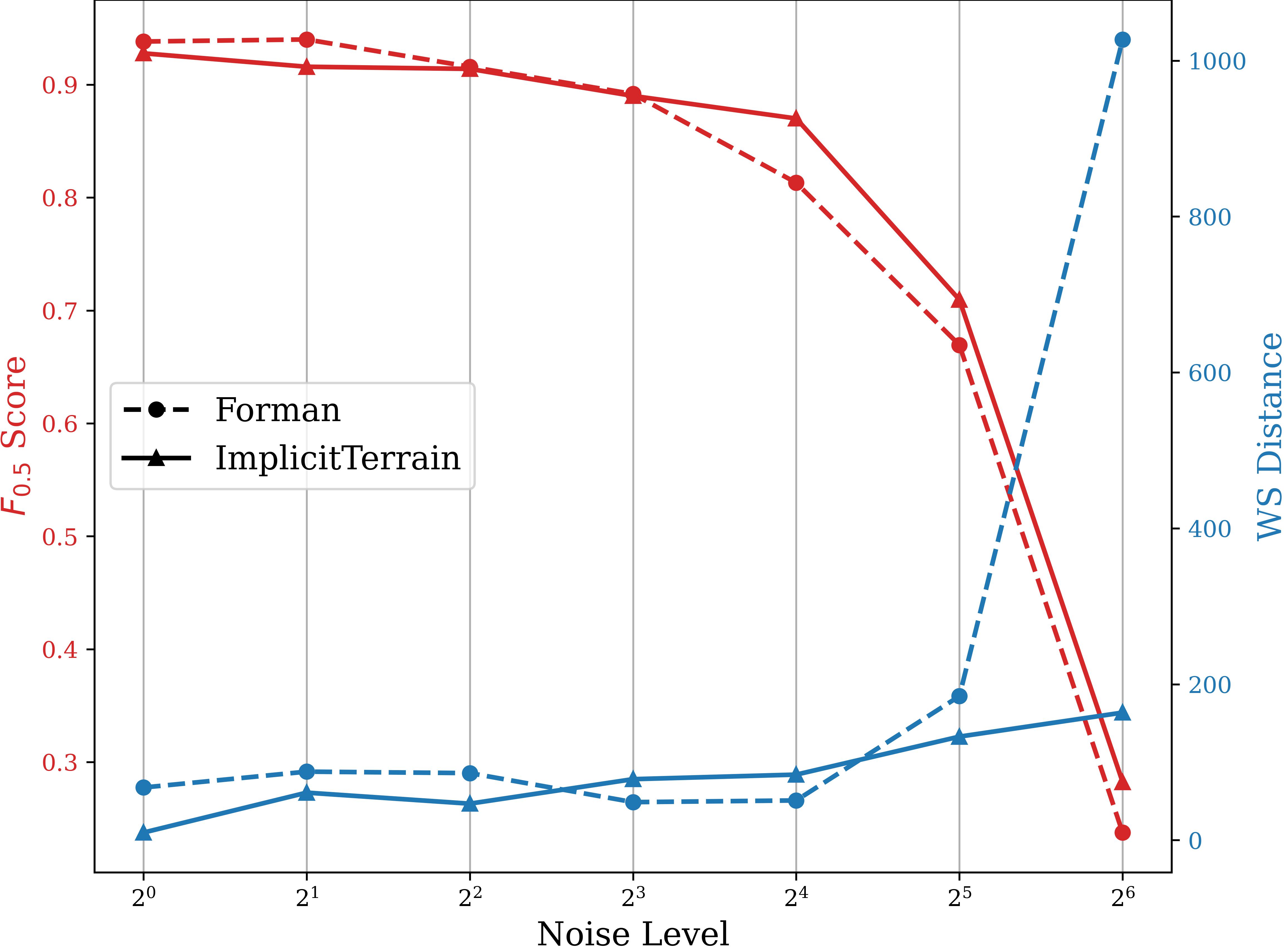
To evaluate the model’s robustness to the presence of noise, pixel-wise Gaussian random noise is added to the normalized input with the variance of noise growing from 1e-3 to 6.4e-2 exponentially. Averaging the results from 5 rounds, Figure 8 shows the changes of $\text{Swiss}_{1}$’s $F_{0.5}$-scores and Wasserstein distance to the reference (original input) with the increment of noise level. ImplicitTerrain achieves on par result with the Forman method at the beginning and shows superior robustness when the noise level further increases.

Figure 8: Comparison of noise robustness. Forman method and ImplicitTerrain comparison via $F_{0.5}$ score and Wasserstein distance of the $\text{Swiss}_{1}$ w.r.t. noise level.

4.6 Terrain topographical analysis

Our ImplicitTerrain, as a smooth model of the terrain surface, can easily support the topographical analysis that requires the computation of surface derivatives [44]. Since the surface function $F(x,y)=z$ is a scalar function defined over the 2D domain, the normal direction can be derived as $\left<-f_{x},-f_{y},1\right>$, where $f_{x},f_{y}$ are the first-order derivatives of the function. According to [50], the mean curvature of the manifold can be derived from the second-order derivative of the function as

$$H=\frac{(1+f_{y}^{2})f_{xx}-2f_{x}f_{y}f_{xy}+(1+f_{x}^{2})f_{yy}}{2(1+f_{x}^{2}+f_{y}^{2})^{3/2}}$$ (5)

where $f_{xx},f_{xy},f_{yy}$ are the second-order derivatives of the function. In the last stage of Fig. 2, we show the basic topographical terrain attributes of $\text{Swiss}_{1}$ derived from the gradient of $\Psi_{s}$, i.e. normal map, slope, aspect, and mean curvature. Limited by the paper length, detailed definition, and high-resolution results in the supplementary materials.

5 Conclusion

In this paper, we propose an ImplicitTerrain pipeline to accurately model high-resolution terrain data and support various downstream analyses over a smooth surface representation. Digital surface model and geometric details are sequentially learned by our Surface-plus-Geometry (SPG) model, in which the surface model fitting is accelerated by a multi-stage learning strategy. Furthermore, the smooth and accurate terrain model enables Morse theory-based topological analysis results to be reliable and interpretable. In the future, we plan to process high-resolution point clouds directly and extend the pipeline to support large-scale terrain regions with better model design. The training time and inferencing computation burden can be further optimized by the meta-learning and model quantization correspondingly. We believe that ImplicitTerrain will benefit many research fields that require accurate surface modeling and topological data analysis.

References

- Atzmon and Lipman [2020] Matan Atzmon and Yaron Lipman. Sal: Sign agnostic learning of shapes from raw data. In Proceedings of the IEEE/CVF conference on computer vision and pattern recognition, pages 2565–2574, 2020.
- Bajaj et al. [1998] Chandrajit L Bajaj, Valerio Pascucci, and Daniel R Schikore. Visualization of scalar topology for structural enhancement. IEEE, 1998.
- Banchoff [1967] Thomas Banchoff. Critical points and curvature for embedded polyhedra. Journal of Differential Geometry, 1(3-4):245–256, 1967.
- Basri et al. [2020] Ronen Basri, Meirav Galun, Amnon Geifman, David W. Jacobs, Yoni Kasten, and Shira Kritchman. Frequency bias in neural networks for input of non-uniform density. In International Conference on Machine Learning, 2020.
- Bemana et al. [2020] Mojtaba Bemana, Karol Myszkowski, Hans-Peter Seidel, and Tobias Ritschel. X-fields: Implicit neural view-, light-and time-image interpolation. ACM Transactions on Graphics (TOG), 39(6):1–15, 2020.
- Catania and Allegra [2023] Lorenzo Catania and Dario Allegra. Nif: A fast implicit image compression with bottleneck layers and modulated sinusoidal activations. Proceedings of the 31st ACM International Conference on Multimedia, 2023.
- Chabra et al. [2020] Rohan Chabra, Jan E Lenssen, Eddy Ilg, Tanner Schmidt, Julian Straub, Steven Lovegrove, and Richard Newcombe. Deep local shapes: Learning local sdf priors for detailed 3d reconstruction. In Computer Vision–ECCV 2020: 16th European Conference, Glasgow, UK, August 23–28, 2020, Proceedings, Part XXIX 16, pages 608–625. Springer, 2020.
- Chen et al. [2021a] Hao Chen, Bo He, Hanyu Wang, Yixuan Ren, Ser-Nam Lim, and Abhinav Shrivastava. Nerv: Neural representations for videos. In Neural Information Processing Systems, 2021a.
- Chen et al. [2022] Hao Chen, M. Gwilliam, Bo He, Ser Nam Lim, and Abhinav Shrivastava. Cnerv: Content-adaptive neural representation for visual data. In British Machine Vision Conference, 2022.
- Chen et al. [2021b] Yinbo Chen, Sifei Liu, and Xiaolong Wang. Learning continuous image representation with local implicit image function. In Proceedings of the IEEE/CVF conference on computer vision and pattern recognition, pages 8628–8638, 2021b.
- Chen and Zhang [2019] Zhiqin Chen and Hao Zhang. Learning implicit fields for generative shape modeling. In Proceedings of the IEEE/CVF Conference on Computer Vision and Pattern Recognition, pages 5939–5948, 2019.
- Chibane et al. [2020a] Julian Chibane, Thiemo Alldieck, and Gerard Pons-Moll. Implicit functions in feature space for 3d shape reconstruction and completion. In Proceedings of the IEEE/CVF conference on computer vision and pattern recognition, pages 6970–6981, 2020a.
- Chibane et al. [2020b] Julian Chibane, Gerard Pons-Moll, et al. Neural unsigned distance fields for implicit function learning. Advances in Neural Information Processing Systems, 33:21638–21652, 2020b.
- Chiu et al. [2021] Pao-Hsiung Chiu, Jian Cheng Wong, Chinchun Ooi, My Ha Dao, and Y. Ong. Can-pinn: A fast physics-informed neural network based on coupled-automatic-numerical differentiation method. ArXiv, abs/2110.15832, 2021.
- Comic et al. [2010] Lidija Comic, Leila De Floriani, and Federico Iuricich. Building Morphological Representations for 2D and 3D Scalar Fields. In Eurographics Italian Chapter Conference 2010. The Eurographics Association, 2010.
- Cuomo et al. [2022] Salvatore Cuomo, Vincenzo Schiano Di Cola, Fabio Giampaolo, Gianluigi Rozza, Maziar Raissi, and Francesco Piccialli. Scientific machine learning through physics–informed neural networks: Where we are and what’s next. Journal of Scientific Computing, 92(3):88, 2022.
- De Floriani et al. [2013] Leila De Floriani, Federico Iuricich, Paola Magillo, and Patricio Simari. Discrete morse versus watershed decompositions of tessellated manifolds. In Image Analysis and Processing–ICIAP 2013: 17th International Conference, Naples, Italy, September 9-13, 2013, Proceedings, Part II 17, pages 339–348. Springer, 2013.
- De Floriani et al. [2015] Leila De Floriani, Ulderico Fugacci, Federico Iuricich, and Paola Magillo. Morse complexes for shape segmentation and homological analysis: discrete models and algorithms. In Computer graphics forum, pages 761–785. Wiley Online Library, 2015.
- Delaunay et al. [1934] Boris Delaunay et al. Sur la sphere vide. Izv. Akad. Nauk SSSR, Otdelenie Matematicheskii i Estestvennyka Nauk, 7(793-800):1–2, 1934.
- Derksen and Izzo [2021] Dawa Derksen and Dario Izzo. Shadow neural radiance fields for multi-view satellite photogrammetry. In Proceedings of the IEEE/CVF Conference on Computer Vision and Pattern Recognition, pages 1152–1161, 2021.
- Dey et al. [2017] Tamal K Dey, Jiayuan Wang, and Yusu Wang. Improved road network reconstruction using discrete morse theory. In Proceedings of the 25th ACM SIGSPATIAL international conference on advances in geographic information systems, pages 1–4, 2017.
- Du et al. [2021] Yilun Du, Yinan Zhang, Hong-Xing Yu, Joshua B Tenenbaum, and Jiajun Wu. Neural radiance flow for 4d view synthesis and video processing. In 2021 IEEE/CVF International Conference on Computer Vision (ICCV), pages 14304–14314. IEEE Computer Society, 2021.
- Dupont et al. [2021] Emilien Dupont, Adam Goli’nski, Milad Alizadeh, Yee Whye Teh, and A. Doucet. Coin: Compression with implicit neural representations. ArXiv, abs/2103.03123, 2021.
- Fathony et al. [2020] Rizal Fathony, Anit Kumar Sahu, Devin Willmott, and J Zico Kolter. Multiplicative filter networks. In International Conference on Learning Representations, 2020.
- Fellegara et al. [2014] Riccardo Fellegara, Federico Luricich, Leila De Floriani, and Kenneth Weiss. Efficient computation and simplification of discrete morse decompositions on triangulated terrains. In Proceedings of the 22nd ACM SIGSPATIAL International Conference on Advances in Geographic Information Systems, pages 223–232, 2014.
- Fellegara et al. [2017] Riccardo Fellegara, Federico Iuricich, and Leila De Floriani. Efficient representation and analysis of triangulated terrains. In Proceedings of the 25th ACM SIGSPATIAL International Conference on Advances in Geographic Information Systems, pages 1–4, 2017.
- Fellegara et al. [2023] Riccardo Fellegara, Federico Iuricich, Yunting Song, and Leila De Floriani. Terrain trees: a framework for representing, analyzing and visualizing triangulated terrains. GeoInformatica, 27(3):525–564, 2023.
- Forman [1998] Robin Forman. Morse theory for cell complexes. Advances in mathematics, 134(1):90–145, 1998.
- Fugacci et al. [2016] Ulderico Fugacci, Sara Scaramuccia, Federico Iuricich, Leila De Floriani, et al. Persistent homology: a step-by-step introduction for newcomers. In STAG, pages 1–10, 2016.
- Genova et al. [2020] Kyle Genova, Forrester Cole, Avneesh Sud, Aaron Sarna, and Thomas Funkhouser. Local deep implicit functions for 3d shape. In Proceedings of the IEEE/CVF Conference on Computer Vision and Pattern Recognition, pages 4857–4866, 2020.
- Gilbert [1991] George T Gilbert. Positive definite matrices and sylvester’s criterion. The American Mathematical Monthly, 98(1):44–46, 1991.
- Gropp et al. [2020] Amos Gropp, Lior Yariv, Niv Haim, Matan Atzmon, and Yaron Lipman. Implicit geometric regularization for learning shapes. arXiv preprint arXiv:2002.10099, 2020.
- Gyulassy et al. [2008] Attila Gyulassy, Peer-Timo Bremer, Bernd Hamann, and Valerio Pascucci. A practical approach to morse-smale complex computation: Scalability and generality. IEEE Transactions on Visualization and Computer Graphics, 14(6):1619–1626, 2008.
- Henzler et al. [2020] Philipp Henzler, Niloy J Mitra, and Tobias Ritschel. Learning a neural 3d texture space from 2d exemplars. In Proceedings of the IEEE/CVF Conference on Computer Vision and Pattern Recognition, pages 8356–8364, 2020.
- Hornik [1991] Kurt Hornik. Approximation capabilities of multilayer feedforward networks. Neural networks, 4(2):251–257, 1991.
- Jiang et al. [2022] Boyan Jiang, Xinlin Ren, Mingsong Dou, Xiangyang Xue, Yanwei Fu, and Yinda Zhang. Lord: Local 4d implicit representation for high-fidelity dynamic human modeling. In European Conference on Computer Vision, pages 307–326. Springer, 2022.
- Jiang et al. [2020] Chiyu Jiang, Avneesh Sud, Ameesh Makadia, Jingwei Huang, Matthias Nießner, Thomas Funkhouser, et al. Local implicit grid representations for 3d scenes. In Proceedings of the IEEE/CVF Conference on Computer Vision and Pattern Recognition, pages 6001–6010, 2020.
- Lin et al. [2020] Chen-Hsuan Lin, Chaoyang Wang, and Simon Lucey. Sdf-srn: Learning signed distance 3d object reconstruction from static images. Advances in Neural Information Processing Systems, 33:11453–11464, 2020.
- Lindell et al. [2022] David B Lindell, Dave Van Veen, Jeong Joon Park, and Gordon Wetzstein. Bacon: Band-limited coordinate networks for multiscale scene representation. In Proceedings of the IEEE/CVF conference on computer vision and pattern recognition, pages 16252–16262, 2022.
- Luo et al. [2023] Jinming Luo, Lei Han, Xianjie Gao, Xiuping Liu, and Weiming Wang. Sr-feinr: Continuous remote sensing image super-resolution using feature-enhanced implicit neural representation. Sensors, 23(7):3573, 2023.
- Mahammad and Ramakrishnan [2003] Sk Sazid Mahammad and R Ramakrishnan. Geotiff-a standard image file format for gis applications. Map India, pages 28–31, 2003.
- Mescheder et al. [2019] Lars Mescheder, Michael Oechsle, Michael Niemeyer, Sebastian Nowozin, and Andreas Geiger. Occupancy networks: Learning 3d reconstruction in function space. In Proceedings of the IEEE/CVF conference on computer vision and pattern recognition, pages 4460–4470, 2019.
- Milnor [1963] John Willard Milnor. Morse theory. Number 51. Princeton university press, 1963.
- Mitášová and Mitáš [1993] Helena Mitášová and Lubos Mitáš. Interpolation by regularized spline with tension: I. theory and implementation. Mathematical geology, 25:641–655, 1993.
- Molaei et al. [2023] Amirali Molaei, Amirhossein Aminimehr, Armin Tavakoli, Amirhossein Kazerouni, Bobby Azad, Reza Azad, and Dorit Merhof. Implicit neural representation in medical imaging: A comparative survey. In Proceedings of the IEEE/CVF International Conference on Computer Vision, pages 2381–2391, 2023.
- Müller et al. [2022] Thomas Müller, Alex Evans, Christoph Schied, and Alexander Keller. Instant neural graphics primitives with a multiresolution hash encoding. ACM Transactions on Graphics (ToG), 41(4):1–15, 2022.
- Niemeyer and Geiger [2021] Michael Niemeyer and Andreas Geiger. Giraffe: Representing scenes as compositional generative neural feature fields. In Proceedings of the IEEE/CVF Conference on Computer Vision and Pattern Recognition, pages 11453–11464, 2021.
- Niemeyer et al. [2020] Michael Niemeyer, Lars Mescheder, Michael Oechsle, and Andreas Geiger. Differentiable volumetric rendering: Learning implicit 3d representations without 3d supervision. In Proceedings of the IEEE/CVF Conference on Computer Vision and Pattern Recognition, pages 3504–3515, 2020.
- Oechsle et al. [2019] Michael Oechsle, Lars Mescheder, Michael Niemeyer, Thilo Strauss, and Andreas Geiger. Texture fields: Learning texture representations in function space. In Proceedings of the IEEE/CVF International Conference on Computer Vision, pages 4531–4540, 2019.
- O’neill [2006] Barrett O’neill. Elementary differential geometry. Elsevier, 2006.
- Park et al. [2019] Jeong Joon Park, Peter Florence, Julian Straub, Richard Newcombe, and Steven Lovegrove. Deepsdf: Learning continuous signed distance functions for shape representation. In Proceedings of the IEEE/CVF conference on computer vision and pattern recognition, pages 165–174, 2019.
- Paz et al. [2022] Hallison Paz, Tiago Novello, Vinicius Silva, Guilherme Schardong, Luiz Schirmer, Fabio Chagas, Helio Lopes, and Luiz Velho. Multiresolution neural networks for imaging. In 2022 35th SIBGRAPI Conference on Graphics, Patterns and Images (SIBGRAPI), pages 174–179. IEEE, 2022.
- Peng et al. [2020] Songyou Peng, Michael Niemeyer, Lars Mescheder, Marc Pollefeys, and Andreas Geiger. Convolutional occupancy networks. In Computer Vision–ECCV 2020: 16th European Conference, Glasgow, UK, August 23–28, 2020, Proceedings, Part III 16, pages 523–540. Springer, 2020.
- Rahaman et al. [2018] Nasim Rahaman, Aristide Baratin, Devansh Arpit, Felix Dräxler, Min Lin, Fred A. Hamprecht, Yoshua Bengio, and Aaron C. Courville. On the spectral bias of neural networks. In International Conference on Machine Learning, 2018.
- Robins et al. [2011] Vanessa Robins, Peter John Wood, and Adrian P Sheppard. Theory and algorithms for constructing discrete morse complexes from grayscale digital images. IEEE Transactions on pattern analysis and machine intelligence, 33(8):1646–1658, 2011.
- Saito et al. [2019] Shunsuke Saito, Zeng Huang, Ryota Natsume, Shigeo Morishima, Angjoo Kanazawa, and Hao Li. Pifu: Pixel-aligned implicit function for high-resolution clothed human digitization. In Proceedings of the IEEE/CVF international conference on computer vision, pages 2304–2314, 2019.
- Schneider [2005] Bernhard Schneider. Extraction of hierarchical surface networks from bilinear surface patches. Geographical Analysis, 37(2):244–263, 2005.
- Schneider and Wood [2004] Bernhard Schneider and Jo Wood. Construction of metric surface networks from raster-based dems. Topological Data Structures for Surfaces: An Introduction to Geographical Information Science, pages 53–70, 2004.
- Scoville [2019] Nicholas A Scoville. Discrete Morse Theory. American Mathematical Soc., 2019.
- Shivashankar et al. [2011] Nithin Shivashankar, M Senthilnathan, and Vijay Natarajan. Parallel computation of 2d morse-smale complexes. IEEE Transactions on Visualization and Computer Graphics, 18(10):1757–1770, 2011.
- Sitzmann et al. [2019] Vincent Sitzmann, Michael Zollhöfer, and Gordon Wetzstein. Scene representation networks: Continuous 3d-structure-aware neural scene representations. Advances in Neural Information Processing Systems, 32, 2019.
- Sitzmann et al. [2020] Vincent Sitzmann, Julien Martel, Alexander Bergman, David Lindell, and Gordon Wetzstein. Implicit neural representations with periodic activation functions. Advances in neural information processing systems, 33:7462–7473, 2020.
- Strümpler et al. [2021] Yannick Strümpler, Janis Postels, Ren Yang, Luc Van Gool, and Federico Tombari. Implicit neural representations for image compression. In European Conference on Computer Vision, 2021.
- Stucker et al. [2022] Corinne Stucker, Bingxin Ke, Yuanwen Yue, Shengyu Huang, Iro Armeni, and Konrad Schindler. Implicity: City modeling from satellite images with deep implicit occupancy fields. arXiv preprint arXiv:2201.09968, 2022.
- Swisstopo [2023] Swisstopo. Swissalti3d datasets. https://www.swisstopo.admin.ch/en/height-model-swissalti3d, 2023.
- Tancik et al. [2020] Matthew Tancik, Pratul Srinivasan, Ben Mildenhall, Sara Fridovich-Keil, Nithin Raghavan, Utkarsh Singhal, Ravi Ramamoorthi, Jonathan Barron, and Ren Ng. Fourier features let networks learn high frequency functions in low dimensional domains. Advances in Neural Information Processing Systems, 33:7537–7547, 2020.
- Tierny et al. [2017] Julien Tierny, Guillaume Favelier, Joshua A Levine, Charles Gueunet, and Michael Michaux. The topology toolkit. IEEE transactions on visualization and computer graphics, 24(1):832–842, 2017.
- Wang et al. [2021] Peng Wang, Lingjie Liu, Yuan Liu, Christian Theobalt, Taku Komura, and Wenping Wang. Neus: Learning neural implicit surfaces by volume rendering for multi-view reconstruction. arXiv preprint arXiv:2106.10689, 2021.
- Weiss et al. [2013] Kenneth Weiss, Federico Iuricich, Riccardo Fellegara, and Leila De Floriani. A primal/dual representation for discrete morse complexes on tetrahedral meshes. In Computer Graphics Forum, pages 361–370. Wiley Online Library, 2013.
- Xiangli et al. [2022] Yuanbo Xiangli, Linning Xu, Xingang Pan, Nanxuan Zhao, Anyi Rao, Christian Theobalt, Bo Dai, and Dahua Lin. Bungeenerf: Progressive neural radiance field for extreme multi-scale scene rendering. In European conference on computer vision, pages 106–122. Springer, 2022.
- Xie et al. [2022] Yiheng Xie, Towaki Takikawa, Shunsuke Saito, Or Litany, Shiqin Yan, Numair Khan, Federico Tombari, James Tompkin, Vincent Sitzmann, and Srinath Sridhar. Neural fields in visual computing and beyond. In Computer Graphics Forum, pages 641–676. Wiley Online Library, 2022.
- Xu et al. [2019] Qiangeng Xu, Weiyue Wang, Duygu Ceylan, Radomir Mech, and Ulrich Neumann. Disn: Deep implicit surface network for high-quality single-view 3d reconstruction. Advances in neural information processing systems, 32, 2019.
- Xu et al. [2023] Xin Xu, Federico Iuricich, Kim Calders, John Armston, and Leila De Floriani. Topology-based individual tree segmentation for automated processing of terrestrial laser scanning point clouds. International Journal of Applied Earth Observation and Geoinformation, 116:103145, 2023.
- Yang et al. [2023] Runzhao Yang, Tingxiong Xiao, Yuxiao Cheng, Qianni Cao, Jinyuan Qu, Jinli Suo, and Qionghai Dai. Sci: A spectrum concentrated implicit neural compression for biomedical data. In Proceedings of the AAAI Conference on Artificial Intelligence, pages 4774–4782, 2023.
- Yariv et al. [2021] Lior Yariv, Jiatao Gu, Yoni Kasten, and Yaron Lipman. Volume rendering of neural implicit surfaces. Advances in Neural Information Processing Systems, 34:4805–4815, 2021.
- Yifan et al. [2021] Wang Yifan, Lukas Rahmann, and Olga Sorkine-Hornung. Geometry-consistent neural shape representation with implicit displacement fields. arXiv preprint arXiv:2106.05187, 2021.
- Yüce et al. [2022] Gizem Yüce, Guillermo Ortiz-Jiménez, Beril Besbinar, and Pascal Frossard. A structured dictionary perspective on implicit neural representations. In Proceedings of the IEEE/CVF Conference on Computer Vision and Pattern Recognition, pages 19228–19238, 2022.