Lessons from the high-resolution spectroscopy of AW UMa and $\epsilon\,$CrA:
Is the Lucy model valid?

Abstract

A re-examination of high-resolution spectral monitoring of the W UMa-type binaries AW UMa and $\epsilon\,$CrA casts doubt on the widely utilized Lucy (1968a, b) model of contact binaries. The detection of the very faint profile of the secondary component in AW UMa leads to a new spectroscopic determination of the mass ratio, $q_{\rm sp}=0.092\pm 0.007$, which is close to the previous, medium-resolution spectroscopic result of Pribulla & Rucinski (2008), $q_{\rm sp}=0.101\pm 0.006$, and remains substantially different from a cluster of generally accepted photometric results by several authors, concentrated around $q_{\rm ph}=0.080\pm 0.005$. The two approaches are independent, with the spectroscopic technique being more direct yet more demanding on telescope/spectrograph resources, while the photometric determinations are accessible to smaller telescopes but entirely dependent on the Lucy model. A survey of binaries with the best-determined values of the mass ratio shows a common tendency for $q_{\rm ph}<q_{\rm sp}$. The tendency for systematically smaller values of $q_{\rm ph}$ may result from the overfilling of the primary lobe and underfilling of the secondary lobe relative to the Roche model geometry, as predicted by the Stȩpień (2009) model; the tendency may be variable in time. Despite the observed moderate inter-systemic velocities, the photometric Lucy model may remain useful in providing approximate, though biased, results for the mass ratio. A complicating factor in detailed spectral analysis may be the occurrence of Enhanced Spectral-line Perturbations (ESP) projected over the secondary profiles, appearing in different numbers in the two studied binaries. The ESPs are tentatively identified within the Stȩpień model as collision fronts or fountains of hot, primary-component gas from the circumbinary, energy-carrying flow.

1 Introduction

This paper is a combined re-discussion of the high spectral-resolution time monitoring of two W UMa-type binary stars, AW UMa (Rucinski, 2015, paper P1) and $\epsilon\,$CrA (Rucinski, 2020, paper P2). The binaries are located at the high-mass, long-period end of the W UMa-binary effective-temperature sequence. Excellent introductions to the current state of research on W UMa-type or contact binaries can be found in Gazeas & Stȩpień (2008) and Gazeas (2024).

The W UMa binaries, sometimes also called “contact binaries”, consist of apparently Main Sequence stars in the spectral range from early F-type to early K-type. W UMa binaries are moderately common in the solar vicinity, with one such system per about 500 F-K dwarfs (Rucinski, 2002a). Their kinematic and metallicity properties are characteristic of the old disk population (Rucinski et al., 2013a). The high-luminosity detection advantage of the early F-type systems, such as AW UMa and $\epsilon\,$CrA, compensates for their smaller numbers compared with somewhat later counterparts and for a tendency to have more dissimilar components, resulting in small variability amplitudes. The mass ratios $q=M_{2}/M_{1}$ tend to peak in a wide range around $q\simeq 0.3-0.5$ for more common late-F and early-G type binaries, but rarer early-F systems tend to show small values of $q$ and consequently small light variations. There may exist a bifurcation in the mass ratio as a function of the orbital period (Rucinski, 2010, Fig.6); this matter is currently a subject of further research (Gazeas, 2024).

The similarity of our two targets was not accidental but resulted from a limited availability of telescopes equipped with efficient high-resolution spectrographs that could be used for extended time-monitoring programs. The two objects in question are the brightest W UMa binaries in the sky (with magnitudes $V=6.8$ and 4.8) making them suitable for observation with a signal-to-noise per spectral-resolution element of around one hundred over a few consecutive nights. Such time-monitoring is resource-expensive, and it is possible that the two objects will remain the only ones observed in this manner for the foreseeable future. This paper brings a comparison and rediscussion of the results from P1 and P2, highlighting that rapid spectral monitoring is one of the few avenues for advancing the currently somewhat stalled research on the validity of the popular Lucy (1968a, b) model for W UMa-type binaries (Webbink, 2003), especially considering the new, attractive, yet unstudied model proposed by Stȩpień (2009).

In both of the considered here binaries, the early-F type primary component dominates over its smaller companion in terms of the mass and size. Because of its small mass, approximately ten times smaller in both cases, the secondary is an energetically inert appendage to the primary. It carries the binary angular momentum, produces strong tidal effects and provides a substantial surface area for the combined radiative losses of the system. The two binaries are typical for the W UMa-type binaries in that their secondary components appear as hot as the primaries. This characteristic is unique among binary stars with unequal mass components and is the main defining feature of the W UMa-type binaries.

The small masses and unexpectedly high effective temperatures of the secondary components in apparently stable W UMa-type systems emphasize the need to determine the mass ratios $q$ with high accuracy. Ideally, these determinations should involve as few initial assumptions as possible. Currently, many determinations of the mass ratios are based on light-curve-synthesis photometric solutions which utilize the relatively complex Lucy (1968a, b) model, where $q_{\rm ph}$ is one of its many parameters. In contrast, spectroscopic determinations, through a ratio of orbital semi-amplitudes, $q_{\rm sp}=K_{1}/K_{2}$, are expected to reflect global binary dynamics directly but are observationally more challenging to determine.

This paper focuses particularly on the observational properties of the secondary components and the energy-transport mechanisms that lead to their high effective temperatures. We also address the good agreement between the photometric and spectroscopic determinations for $\epsilon\,$CrA at $q=0.13$ (Section 3) and the continuing substantial discrepancy for AW UMa (Section 4). For AW UMa, the medium-resolution result of Pribulla & Rucinski (2008), $q_{\rm sp}=0.101\pm 0.006$, significantly differs from the widely accepted $q_{\rm ph}\simeq 0.08$, based on several photometric studies starting from Mochnacki & Doughty (1972a) and ending with Wilson (2008).

We note that before P1, there have been several previous short-duration attempts to observe AW UMa spectroscopically (Paczyński, 1964; McLean, 1981; Anderson et al., 1983; Rensing et al., 1985; Rucinski, 1992), These efforts mainly focused on detecting the spectroscopically faint secondary component and confirming the photometric mass ratio. The DDO analysis of Pribulla & Rucinski (2008) was the first to provide a larger amount of data. In contrast, $\epsilon\,$CrA was analyzed spectroscopically using a cross-correlation function (CCF) approach only once by Goecking & Duerbeck (1993), followed by the high-quality high-resolution spectral analysis reported in P2. The previous line-by-line measurements for the primary component of $\epsilon\,$CrA by Tapia & Whelan (1975) currently have limited value.

A general description and comparison of both binaries in terms of their general properties is in Section 2. Sections 3 and 4 discuss the complex appearance of the secondary components as seen in spectroscopy. In these sections, the new term Enhanced Spectral-line Perturbation (ESP) is introduced to describe radial-velocity-defined features of increased density of the primary-component gas, projected onto the secondary component profile. A newly detected, very faint signature of the secondary component in AW UMa confirms the “large” value of $q_{\rm sp}$ of about 0.10.

Section 5 demonstrates that the tendency for $q_{\rm ph}<q_{\rm sp}$ is a common feature in the best mass-ratio determinations of other W UMa binaries. As discussed in Section 7, this tendency cannot be explained by the Lucy model but is consistent with the Stȩpień (2009) model. Section 8 discusses the implications of the presented results and suggests possible directions for future research.

2 The two binaries as seen in radial velocities

All results presented in papers P1 and P2 were based on the radial velocity (RV) profiles obtained through the analysis of individual spectra using the linear, Broadening-Functions (BF) deconvolution technique (Rucinski, 2002b, 2010, 2012). The technique is computationally more demanding than the inherently non-linear, easier-to-implement Cross-Correlation Function (CCF) technique; it provides high-quality RV profiles in reference to the shape and strength of the spectral lines for a star of the same spectral type. However, the BF profiles should not be interpreted as RV-projected images of a binary system; to do so, an assumption of a solid-body rotation is necessary; generally, we do not know the spatial location of a given RV feature. Strict solid-body rotation is a basic assumption of the Lucy model, yet determining the correct model is precisely the main subject of our investigation.

As with other spectral deconvolution process, the BF technique has the limitation of being sensitive to the presence of dispersed matter in the binary system: Any emission component in observed line spectra would produce a dip or would weaken the restored velocity profile, while any absorption would produce stronger features in BF profiles. In general, deviations from a standard, stellar-atmosphere optical-depth dependence of the source function can modify the profile. The BF technique, thanks to its linear properties, tends to show such deviations more directly than the CCF technique.

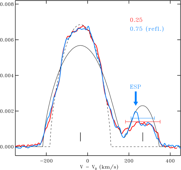
Figure 1: The BF profiles for $\epsilon\,$CrA at both orbital quadratures, i.e. phases $\phi=0.25$ (red) and $\phi=0.75$ (blue), in units per a RV sampling interval of 8.5 km s^-1. The profile $\phi=0.75$ is inverted in the velocity scale with the common origin at the RV of the binary mass center at $V_{0}=-62.54$ km s^-1. The Lucy-model profile for the orbital phase $\phi=0.25$ and the assumed mass ratio $q=0.13$, the fill-out parameter $f=0.25$ is shown by a thin black line. Vertical dashes mark the mass-center RV’s while a thin, broken line shows the rotational profile fit to the primary component. The red and blue bars over the secondary component show the widths of the secondary profile observed at both orbital quadratures. An Enhanced Spectral-line Perturbation (ESP) affecting the secondary profile at $\phi=0.75$ is pointed by an arrow at 235 km s^-1.

The data for AW UMa (P1) and $\epsilon\,$CrA (P2) were analyzed with the spectra resampled to the same spectral resolution of 8.5 km s^-1 (the resolving power $R\simeq 35,\!000$), with the final RV profiles for $\epsilon\,$CrA being of much better quality: The median signal-to-noise ratio per resolution element of $S/N=57$ was for AW UMa (P1) and $S/N=120$ for $\epsilon\,$CrA (P2). We show two typical RV profiles for $\epsilon\,$CrA at both orbital quadratures in Figure 1. Typical profiles for AW UMa are very similar, but are much more complex and variable within the secondary component parts and exhibit larger observational noise.

Here is a summary of similarities and differences between the two binaries:

1. In both stars, the upper two-thirds of the primary component profile is narrower than predicted by the Lucy contact-binary model but agrees very well with a standard profile for a single star rotating at about 80% – 85% of the orbit-synchronous rotation rate. This property was recognized in AW UMa already by Rensing et al. (1985) using photographic spectra. The base of the primary profile in both binaries referred to as the “pedestal” in P1, is approximately as wide, as predicted by the Lucy model. The narrow primary profile may be due to the anticyclonic circulation around the rotation pole of the mass-losing primary, as predicted by the hydrodynamic model of Oka et al. (2002), while the wide pedestal is explained by the binary circulation model of Stȩpień (2009). These observational properties contribute to our discussion of an appropriate model for W UMa binaries in Section 7.

2. In both stars, the primary $V\sin i$ widths show a very small tidal (ellipsoidal) component of $<5$ km s^-1, in comparison to their mean values of $\simeq 181$ km s^-1 in AW UMa (P1, Fig. 3) and $\simeq 147$ km s^-1 in $\epsilon\,$CrA (P2, Fig. 3). The tidal variations are partly masked by greater noise in AW UMa but are better defined in $\epsilon\,$CrA.

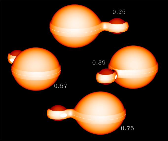
Figure 10: A schematic view of $\epsilon\,$CrA at four orbital phases envisaged for the Stȩpień model; compare it with Figure 3 for the Lucy model. The belt surrounding both stars is pictured here with an arbitrary height of $\pm 0.1$ orbital separation units; its temperature is set slightly higher than at the side of the primary for better visibility. For a simpler visual representation, all shown surfaces follow the equipotentials: the primary is at the inner critical one, the secondary at the one with the side radius 0.95 of its inner critical, while the belt is positioned at a half-way between the inner and outer critical equipotentials.

3. The primary component of AW UMa showed a network of “ripples” or non-radial pulsations partly extending into the profile pedestal. The ripples, which are visible after subtraction of the stable mean profile (Figures 8, 9, 10 in P1), look very similar to the non-radial pulsations detected (subsequently to the work reported in P1) in the rapidly rotating, bright star Altair ($\alpha$ Aql, A7V, $V\sin i\simeq 240$ km s^-1; Rieutord et al. (2023)).

   The primary of $\epsilon\,$CrA appears to be entirely free of such non-radial pulsations; they would be easily detectable because of the higher $S/N$ of its spectra.

4. The secondary-component RV profiles of both binaries appeared much weaker and flatter than expected by the Lucy model. This could indicate a genuine faintness of the secondaries or a different (later) spectrum, not matching the template used in the BF determination.

5. The secondary-component profiles in both binaries were distorted by localized perturbations which systematically shifted with the orbital phase. The disturbances, referred to as “wisps” in P1 and P2 due to their visibility in time-sequences of the RV profiles, complicated our interpretation of the secondary component shape in AW UMa; see their confusing appearance in Figure 13 in P1.

   $\epsilon\,$CrA (P2) showed only one “wisp”. Its phase evolution could be interpreted as due to a localized region of hotter (i.e.  primary-component) gas overlying the secondary component profile. Its location was estimated at the sub-observer orbital phase $\phi=0.65$ and may correspond to a collision front of the gas striking the primary after circulating the secondary component. The disturbance was very stable and remained visible during the whole observing run of the 28 orbital revolutions of $\epsilon\,$CrA. It is marked by an arrow in the $\phi=0.75$ profile in Figure 1; its orbital-phase evolution is discussed in Section 3. In this paper, we introduce the term Enhanced Spectral-line Perturbations (ESP) to stress that such perturbations in Broadening Function profiles correspond to stronger absorption spectra due to more gas atoms having the same atomic excitation properties as assumed for the early-F type template.

6. The better data quality and somewhat simpler profiles permitted the detection of weakly defined outermost edges of the secondary-component velocity profile in $\epsilon\,$CrA (P2). Since both edges were detected, the velocity field on the secondary seemed to be well confined, similar to that of a detached star. The mean velocity from the edges – assumed to be that of the secondary mass center – showed an approximately sine-curve phase dependence, as expected in anti-phase to that observed for the primary component. The semi-amplitude $K_{2}$ derived in this way led to a mass ratio $q_{\rm sp}=K_{1}/K_{2}=0.130\pm 0.001$, in general consistency with the photometric Lucy-model estimates, $q_{\rm ph}=0.114\pm 0.003$ (Twigg, 1979) and $0.1244\pm 0.0014$ (Wilson & Raichur, 2011). Unfortunately, a similar direct determination of $K_{2}$ for AW UMa in P1 could not be done due to the simultaneous presence of several ESPs affecting the secondary-component profile. Indirect estimates in P1, based on the poorly-defined mean profile shape suggested a value of the mass ratio $q_{\rm sp}\simeq 0.10$.

7. The edge-to-edge widths of the $\epsilon\,$CrA secondary-component RV profile appeared to differ for the two orbital quadratures. Expressed as the observed half-widths, they were approximately 90 km s^-1 at $\phi=0.25$ and 70 km s^-1 $\phi=0.75$. This unexplained variability is marked by horizontal bars over the secondary-component profiles in Figure 1. This subject is discussed further in Section 3.

8. No parallel photometry was conducted during the spectroscopic programs described in P1 and P2. Information restored from the available spectra (Figure 2 in P1; Figure 13 in P2) reveals different and complex phase variations of the integrated strength of all spectral lines in the used BF window for the two binaries.

9. The spectroscopic data do not provide information on the orbital inclinations of either binary. A difference in the photometric variability amplitudes suggests that the $\epsilon\,$CrA orbit is viewed at a slightly more inclined angle than AW UMa. The tentative assumptions of the previous, Lucy-model photometric estimates (Sec. 1) are $i\simeq 78^{\circ}-80^{\circ}$ for AW UMa and $i\simeq 72^{\circ}-73^{\circ}$ for $\epsilon\,$CrA, though these are not explicitly used in the paper. It may be useful to note that for $\epsilon\,$CrA, we can possibly observe the volume between the components during the transit eclipse ($\phi=0$), with a line-of-sight passing “above” the secondary component (see Figure 3).

10. Although they have the same spectral type and a similar, small mass ratio, the binaries are definitely not identical: Their orbital periods differ substantially: 0.4387 days for AW UMa and 0.5914 days for $\epsilon\,$CrA. The observed maximum-light $V$ magnitudes are 6.84 and 4.74, and the parallax data, 14.78 mas and 31.81 mas for AW UMa and $\epsilon\,$CrA respectively (Gaia Collaboration, 2020). These values give the absolute maximum-light magnitudes $M_{V}=2.69$ for AW UMa and 2.25 for $\epsilon\,$CrA. The longer period and the higher luminosity of $\epsilon\,$CrA align with its larger primary mass, as discussed in P1 and P2.

    Both binaries appear to systematically change their orbital periods, showing well-defined parabolic variations in the $O-C$ eclipse moments, but in the opposite sense: In AW UMa the period shortens (Rucinski et al., 2013b), while in $\epsilon\,$CrA the period lengthens (P2). The respective timescales are $(-2.3\pm 0.1)\times 10^{6}$ yrs and $(+1.26\pm 0.04)\times 10^{6}$ yrs. AW UMa has a physical, G7V proper-motion companion $67\arcsec$ away ($>\!4,600$ AU), while no third body has been detected for $\epsilon\,$CrA so far.

3 The secondary component of $\epsilon\,$CrA

The secondary components keep the secret of the moderate mass and large energy transfer between the component stars in W UMa-type systems such as $\epsilon\,$CrA and AW UMa. These processes are critical to understanding the relatively long duration of the contact phase in these systems. The following sections will describe the observed properties of the secondary components, beginning with $\epsilon\,$CrA and then moving on to AW UMa. This sequence deviates from the analysis order in the previous studies (P1 and P2), prioritizing the simpler and more thoroughly observed $\epsilon\,$CrA to more effectively elucidate the shared features. For $\epsilon\,$CrA, we rely on the previously established orbital semi-amplitudes, $K_{1}$ and $K_{2}$, as reported in P2, without any modifications. The focus will be on the lessons learned from the case of $\epsilon\,$CrA and how they could be applied to understanding AW UMa, as discussed in Section 4.

As described in P2, the secondary component was relatively easy to detect in the radial velocity profiles of $\epsilon\,$CrA. While no distinct peak or profile centroid could be detected, the range or extent of the profile was well defined by “edges” on images derived from the RV profiles. The presence of such RV edges made the secondary component profiles dramatically different from that predicted by the Lucy model and resembling those for a velocity field on a detached binary component. The profiles were significantly fainter and flatter than those expected by the Lucy model (Figure 1). However, the extremes of the observed profiles were consistently well-defined to assume that their mean values could correspond to the motion of the secondary mass center. These values varied in anti-phase to the orbital motion of the primary component, allowing the derivation of the semi-amplitude $K_{2}$. This finding stands in stack contrast to the complex appearance of the secondary-component profiles in AW UMa (P1, Figure 13)). However, the differences in data quality and quantity between the studies of $\epsilon\,$CrA and AW UMa could influence this comparison, potentially favoring $\epsilon\,$CrA due to its better data quality and phase coverage.

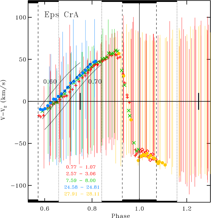
Figure 2: The vertical bars show the edge-to-edge extent of the secondary component RV profiles for $\epsilon\,$CrA, expressed relative to the velocity of the secondary component’s mass center. These measurements are derived from images formed from individual profiles. Observations from individual nights are color-coded as per the legend in the figure, where the integer part of the phase gives the number of elapsed orbits from the assumed initial epoch (see P2). Thick black lines along the upper and lower edges of the figure indicate the phase ranges of the estimated total and partial eclipses. In the left part of the figure, the phase drift of the dominant Enhanced Spectral-line Perturbation (ESP) is represented by colored symbols according to the figure legend. The inclined thin lines alongside these symbols represent the predicted phase drifts for three sub-observer longitudes, expressed in orbital phases: 0.6, 0.65, and 0.7.

The two main complications in the secondary-component profiles of $\epsilon\,$CrA were: (1) The half-extends or half-widths of the profile (functionally similar to $V\sin i$ in rotating stars) showed variations with phase, and (2) a moving, phase-dependent, “spiky” feature, what we call “Enhanced Spectral-line Perturbation” (ESP) was observed in the orbital phases $0.5<\phi<1.0$ (see Figure 1). The first complication was noted only briefly in P2. It is shown in Figure 2 as the full measured extent of the secondary component profile, relative to the assumed sine-curve motion of the secondary with $K_{2}=267$ km s^-1. The widths were determined from images similar to Figures 5 – 9 in P2, rather than from individual RV profiles; this provided a better definition of the measurements. The phase range in Figure 2 is limited to the phases when the secondary component is expected to be in front of the primary, $0.58<\phi<1.42$. Trends in the secondary-component RV widths in Figure 2 appear to be well established: The profile is noticeably narrower ($\simeq 70$ km s^-1) around $\phi\simeq 0.75$ and wider ($\simeq 90$ km s^-1) around $\phi\simeq 0.25$. The deviations from a sine-curve, while relatively small (20 – 30 km s^-1) compared with the large value of $K_{2}$, are definitely systematic. Their presence does not affect the essential anti-symmetric phase variation relative to the primary, yet it is concerning. We do not have a simple explanation for them beyond expectations that the velocity field over the secondary component may be complex and that the outer layers of the secondary are seen at constantly changing orientation and thus optical-depth, oblique-view accumulation.

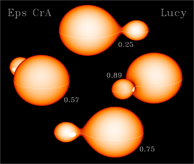
Figure 3: A schematic view of $\epsilon\,$CrA at four orbital phases, as indicated in the figure. The Lucy model with the mass ratio $q=0.13$, the fill-out parameter $f=0.25$ and the orbital inclination $i=73$ degrees were assumed in generating these images. The orbital phases $\phi\simeq 0.57$ and $\phi\simeq 0.89$ correspond to the orientations when the region of the Enhanced Spectral-line Perturbation (ESP), shown as a white patch, comes into view or is about to disappear behind the edge of the secondary component. Except for the approximate location in longitude, the geometry and extent of the ESP-causing region in the stellar latitude are unknown and arbitrary in the figure (see the text).

The second complication of the $\epsilon\,$CrA secondary-component profile, the prominent ESP visible in the phase range $0.57<\phi<0.89$ (Figure 2) requires special attention due to its location, strength and persistence. During each observed binary orbit, the region emerged at $\phi\simeq 0.57$ with the RV around $-10$ km s^-1 relative to the secondary center, then drifted to positive velocities reaching about +55 km s^-1 at $\phi\simeq 0.89$ where it started overlapping with the primary component profile. Constraints on the ESP location within the binary can be derived utilizing the orbital-phase dependence of the RV variations. The simplest model would be a region anchored to the secondary component, with the observed phase variations caused by the variable component of the observer-directed product $\vec{r}\,\Omega$. Here, $\vec{r}$ gives the spatial position of the active ESP region relative to the secondary center and $\Omega$ is the angular rotational velocity of the binary. The inclined lines in Figure 2 give predictions of such a phase dependence for an ESP located on the equator of the secondary component of the inner critical Roche equipotential at three sub-observer points, $\phi=0.60,0.65,0.70$. The zero RV crossing by the drift line suggests a position on the secondary component at the sub-observer position $\phi\simeq 0.65$. Lucy-model generated images of $\epsilon\,$CrA with the ESP located at that longitude are shown for four orbital phases in Figure 3.

To be detected as a positive deviation in the BF, the gas producing the ESP must possess properties similar to those of the outer layers of the primary component, with the same atomic-excitation properties. This is a direct result of the BF determination process which used a high-temperature, early-F type spectrum. The ESP is visible on the hemisphere centered at $\phi=0.75$, which is on the opposite side to where a Coriolis-force-deflected flow from the primary would be expected. Therefore, the stream of matter must have circled the secondary component to collide with some obstacle, forming a fountain or a collision front. We return to this subject in the discussion of the contact binary model in Section 7.

The ESP strength did not seem to vary with the orbital phase within the observed interval $0.57<\phi<0.89$ and remained at an intensity of about 1.5% to 2% ($\pm 0.2\%$) relative to the mean integrated Broadening Function. It was also surprisingly stable over the entire duration of our $\epsilon\,$CrA campaign, remaining at the same place on five observing nights within 28 binary orbits, i.e. for over 2 weeks. Although the active region was placed on the equipotential surface in Figure 3, its spatial location is not well defined; it may be in the space overlying the secondary, possibly as in Figure 9 in the discussion of the Stȩpień model (Section 7.2).

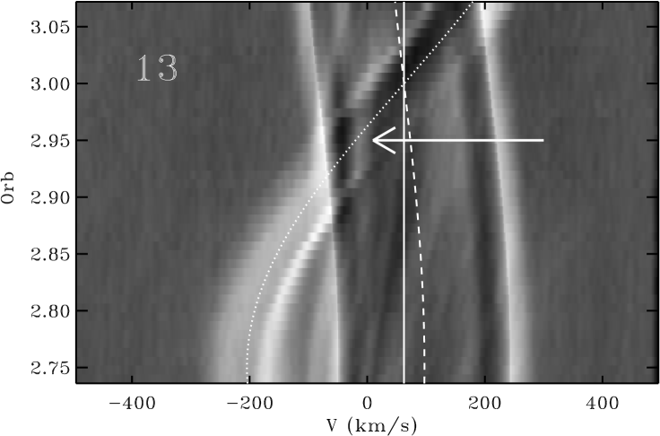
Figure 4: The orbital-phase evolution of the Enhanced Spectral-line Perturbation (ESP) on the secondary component of $\epsilon\,$CrA during the transit eclipse. The horizontal axis shows the radial velocity in the heliocentric system while the vertical axis gives the time (increasing upwards) expressed in orbital periods, $Orb$; the eclipse centre on the observing night #13 was located at $Orb=3.0$ (see P2). The ESP localized at the sub-observer point at $\phi\simeq 0.65$, as described above and in Figure 2, possibly continued its evolution into the eclipse phases and merged with other spectral-line intensity features (see the text). The mass-center velocities of both stars are shown by broken (primary) and dotted (secondary) sine-curve lines.

A detailed analysis of the images formed from the BF profiles for $\epsilon\,$CrA indicated an additional feature in the secondary-component profile that was not discussed in P2: The hot gas that produced the ESP remained at least partially visible during the transit-eclipse phases. As shown in Figure 4, after encountering the primary profile at $\phi\simeq 0.89-0.90$, the ESP stopped shifting in heliocentric radial velocities and stabilized at about $-75$ km s^-1 relative to the binary mass center. This orientation corresponded to the rapid variation of its RV relative to the secondary mass center. All of this happens in projection over the large primary-component disk (Figure 2). Because of the relatively low orbital inclination of $\epsilon\,$CrA of $i\simeq 72^{\circ}-73^{\circ}$, it is possible that – thanks to the line of sight passing above the secondary – we see here the volume between the binary components. This orientation can be visualized for transit-eclipse phases $\phi>0.90$ in Figure 3. From about $\phi\simeq 0.98$ onward, just before the mid-eclipse, the active region became visible at negative velocities (Figure 4), presumably on the observer-approaching side of the secondary component. This may be produced by the new, hot gas from the primary sliding along the surface of the secondary component.

4 The secondary component of AW UMa

The most extensive previous spectroscopic investigation of the AW UMa orbit by Pribulla & Rucinski (2008) was conducted at a medium spectral resolution with data collected at the David Dunlap Observatory (DDO) over ten non-consecutive nights. The mean secondary component profile was used to derive the semi-amplitude $K_{2}$ and then the mass ratio, $q_{\rm sp}=0.101\pm 0.006$. This value was larger than any of the previous Lucy model photometric determinations, which tended to concentrate around $q_{\rm ph}\simeq 0.08$.

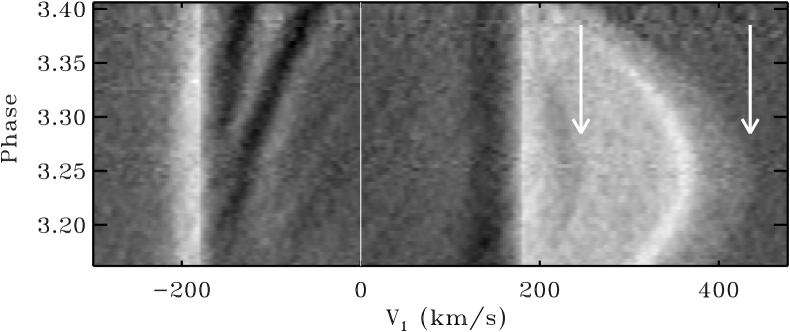
Figure 5: A segment of the 2D image formed from individual BF’s arranged in orbital phase for the second of the available three observing nights of AW UMa; it is a part of Figure 9 in P1. The radial velocities (the horizontal axis) are in the system centered on the primary component with the strong rotational profile of the primary component subtracted from the BF profiles for better visibility of the secondary component. The orbital phases (the vertical axis), are expressed as a full count of orbital cycles from the assumed initial epoch, as in P1. The edges of the secondary component profile, as marked by the arrows, $E_{1}$ and $E_{2}$, were determined from images similar to this one. Note that the strongly non-uniform distribution of intensity across the secondary-component profile and the presence of the bright RV “wisp” which is identified in Figure 7 as ESP #4.

With only three available nights and given a highly complex secondary-component profile, the P1 analysis could provide only a tentative confirmation of the $q_{\rm sp}\simeq 0.10$ result. We re-discuss the results of P1 in light of the experience gained in analyzing the simpler and better-observed $\epsilon\,$CrA binary (Section 3). It should be taken into account that only five orbital revolutions over three nights – with interruptions – were available for AW UMa. As for $\epsilon\,$CrA, a search was made for (1) distinct RV edges of the secondary component profile (as for a detached star) that (2) would move in anti-phase to the motion of the primary component of the binary. They have been detected, but they are less distinct than in $\epsilon\,$CrA due to the presence of several variable ESs (see Figures 8 – 10 of P1). An example of the edges is shown in Figure 5 where they are marked by arrows. The heliocentric velocities of the edges are listed in Table 1.

Table 1: AW UMa: Radial velocities of the secondary-component profile edges

Phase ($Orb$)	$E_{1}$ (km s-1)	$E_{2}$ (km s-1)
0.604	-303.33	-178.28
0.632	-336.09	-206.07
0.636	-334.82	-213.09
0.674	-379.83	-237.40
0.681	-377.60	-243.44

Note. — The first column gives the time expressed in orbital phase counted continuously from the assumed initial epoch (the $Orb$ units, as defined in P1).

The second and third column give the heliocentric radial velocities of the edges of the secondary component profile, $E_{1}$ and $E_{2}$ expressed in km s^-1, as explained in the text.

This table is available in the on-line version only.

Table 2: AW UMa: Orbital solutions

#	$V_{0}$	$K_{1}$	$K_{2}$	Comment
	km s-1	km s-1	km s-1
1	-15.90 ±0.12	28.37 ±0.37		From P1, $0.25<\phi<0.75$, 299 obs.
2	-15.88 ±0.06	29.08 ±0.09		same for $0.20<\phi<0.80$, 340 obs.
3	-14.57 ±1.13		314.06 ±1.18	$0.15<\phi<0.35$ and $0.65<\phi<0.85$, 45 obs.
4	-15.74 ±0.14	29.08 ±0.09	314.32 ±1.17	Combined solution, phases as for #2 and #3.

Note. — The solution uncertainties were estimated as standard ($\pm 1\sigma$) errors by a bootstrap-sampling experiment based on 10,000 repetitions. The bootstrap parameter distributions did not show any obvious asymmetries.

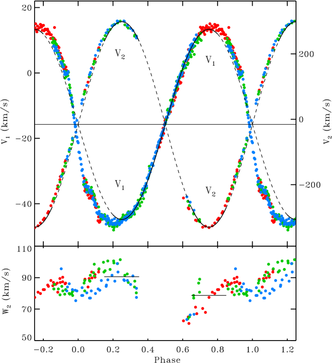
Figure 6: The heliocentric orbital velocities of both AW UMa components. The figure corresponds to Figure 4 in P1, with added velocities of the secondary component, derived as the mean values of the secondary profile edges $E_{1}$ and $E_{2}$. The scale for the secondary (the right vertical axis) is compressed 10 times relative to that for the primary and is shifted to the same $V_{0}$. The three observational nights of AW UMa are coded by color: 1 – red, 2 – green, 3 – blue. The continuous lines give the sine fits to the data in the phase ranges as discussed in the text, with the solid-line portions marking the phase intervals used in the orbital solutions (see the text). The lower panel shows the half-width of the secondary component profile, $W_{2}=(E_{2}-E_{1})/2$, which for a standard rotational profile would correspond to the apparent equatorial velocity $V_{2}\sin i$.

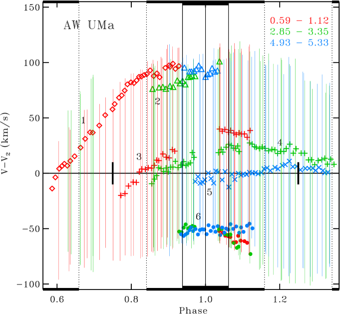
Figure 7: The figure shows the secondary-component profile extent, edge-to-edge, as vertical lines coded in color by the phase range of the observing night; see the legend in the right upper corner of the figure. The velocities are expressed relative to the secondary-component mass center. The horizontal axis shows the orbital phase range centered on the transit (deeper) eclipse. The phase drifts of several Enhanced Spectral-line Perturbations (ESP) are marked by symbols and identified by numbers in the text. The figure is similar to the one for $\epsilon\,$CrA (Figure 2). The thick black marks on the zero-velocity line mark the orbital quadrature phases 0.25 and 0.75 weighing most in the $K_{2}$ determination.

Table 3: The orbital parameters of AW UMa

Parameter	Result	$\pm\sigma$	Unit
$P$	0.4387242		day
$HJD(pri)$	2455631.6498		day
$V_{0}$	-15.74 00	0.14	km s-1
$K_{1}$	29.08	0.09	km s-1
$K_{2}$	314.32 0	1.17	km s-1
$q_{\rm sp}=M_{2}/M_{1}$	0.092	0.007
$A\sin i$	2.977	0.001	$R_{\odot}$
$(M_{1}+M_{2})\sin^{3}i$	1.841	0.019	$M_{\odot}$
$M_{1}\sin^{3}i$	1.685	0.020	$M_{\odot}$
$M_{2}\sin^{3}i$	0.156	0.0026	$M_{\odot}$

Note. — The errors are the formal least-squares errors and do not reflect possible systematic uncertainties in the data.

With the new RV data for the secondary component, we attempted a determination of the spectroscopic orbital elements for AW UMa. Of the available 584 radial velocities for the primary component and 118 measurements for the secondary, the orbital solution used 340 velocities within $0.2<\phi<0.8$ as listed in Table 3 of P1 and all 118 measurements of the profile edges $E_{1}$ and $E_{2}$, as listed in Table 1. The mean values from the edges were used to represent the motion of the secondary component.

The orbital solutions for AW UMa are given in Table 2. The first two lines quote the results for the primary component from P1, while the last line gives the combined final solution for the three parameters $V_{0}$, $K_{1}$ and $K_{2}$. The solution is well-defined thanks to the simultaneous constraint on $V_{0}$ from the motion of both components and the RV’s of the secondary component following the sine curve. The uncertainties of the RV parameters $V_{0}$, $K_{1}$ and $K_{2}$ in Table 2 were determined by bootstrap-sampling experiment. While the formal random errors estimated this way appear to be small, systematic errors may be larger because of the lack of a proper velocity-field description on the stellar disks.

The radial velocity variations for both components are shown in Figure 6. It is similar to Figure 4 in P1, but with the secondary-component orbit added using the velocity scale reduced by 10 times relative to that for the primary component. Table 3 gives the derived parameters of the binary. Please note that the value of $K_{2}$ in Sec. 7.1 of P1 was incorrectly given to the sum of the semi-amplitudes; the correct numbers are given here.

The new radial-velocity solution, as shown in Figure 6, confirms the previously noticed negative deviations of the primary-component radial velocities after the transit mid-eclipse, in the wide phase range $0<\phi<0.25$. Contrary to what was suggested in P1, the RV deviations do not appear to result from the “Rositter – McLaughlin” effect since we see only a trace of positive deviations before the mid-eclipse. Thus, the deviations are asymmetric relative to the line joining the mass centers. The change is forced mostly by the shift in $V_{0}$, caused by the inclusion of the secondary orbit. The phases immediately after the mid-eclipse correspond to the orientation of the binary with the Coriolis-deflected flow from the primary directed at the observer.

The negative RV deviations reach about $-10$ km s^-1 and, surprisingly, the whole, broad profile has acquired such a negative shift as if the whole hemisphere of the primary were approaching the observer. There exists a corresponding negative deviation after the mid-eclipse in $\epsilon\,$CrA (see P2, Fig.4), but it is smaller, on the order of $-3$ km s^-1 and much more localized in the phase range. The current restriction of the AW UMa primary data to the phase range $0.20<\phi<0.80$ is an attempt to eliminate those (poorly understood) profile distortions and thus restore symmetry relative to the line joining the two mass centers.

We note that the primary profiles were observed to briefly broaden during the primary eclipse phases in both binaries (see Fig. 3 in P1 and Fig. 3 in P2), but the width variations seemed to be symmetric relative to the primary eclipse mid-eclipse phase. The findings of the mean velocity shift and the broadening symmetry may be important in understanding the mass outflow from the primary component.

The radial velocities of the secondary component of AW UMa, as derived from the two profile edges $E_{1}$ and $E_{2}$, generally follow the anti-phase variations relative to the primary motion, but with the similar irregularities to those observed in $\epsilon\,$CrA:

1. The half-widths, $W_{2}=(E_{2}-E_{1})/2$, are systematically variable: At the first quadrature $W_{2}(0.25)=91\pm 3$ km s^-1 while at the second quadrature $W_{2}(0.75)=79\pm 3$ km s^-1 (the lower panel of Figure 6);

2. The mean velocities show $\pm 30$ km s^-1 deviations from the expected sine shape (Figure 7); they can be considered moderate relative to the large semi-amplitude $K_{2}=314$ km s^-1, but are systematic.

These irregularities, similar to those observed in $\epsilon\,$CrA (Section 3, Figure 2) probably reflect changes in the spectral-line optical depth for the rapidly changing geometry of the binary system.

While the extent and motion of the underlying secondary-component profiles in AW UMa and $\epsilon\,$CrA appear to be similar, the two binaries differ in the type and number of the ESPs. One strong ESP was visible for $\epsilon\,$CrA on all nights (Figure 2); it always showed the same phase drift as the binary rotated. In contrast, in AW UMa two to four ESPs were simultaneously visible (Figure 7) at different locations within the secondary component profile. One of these was very similar to that in $\epsilon\,$CrA, while the others appeared more irregular showing migration within hours and sometimes reappearing after the observing daytime breaks. The ESPs were typically stronger than the underlying profile; an example, ESP#4, is visible in Figure 5.

The very short period of AW UMa created another complication in attempts to follow the evolution of individual ESPs: expressed in the binary orbital cycles, the CFHT observations experienced relatively long daily breaks amounting to about 1.5 orbital periods of the binary. The observing run was short, lasting only three consecutive nights or five binary revolutions.

Figure 7 shows the ESP phase locations and phase evolution in AW UMa. The apparent equivalent of the single, well-defined feature in $\epsilon\,$CrA, ESP#1, could be observed only on the first night at a similar sub-observer phase $\simeq 0.6-0.65$, as for $\epsilon\,$CrA. It is possible that ESP#2 was a continuation of #1 on the two following nights; its velocities corresponded to the rotationally receding side of the secondary component. The features #3, #4 and #5 appeared at velocities similar to the presumed velocity of the secondary mass center. They tended to drift slightly on all three nights, with the region #5 being most stable at the mean velocity of the secondary. Finally, the repeatable and well-defined ESP#6 was observed at negative velocities; it was most probably produced by the matter moving along the surface of the secondary on its side approaching the observer.

While none of the ESPs can be explained within the Lucy model, the Stȩpień model actually predicts the existence of features such as those given numbers #1 and #6. The ESPs would be manifestations of the stream encompassing the binary system; the sufficiently spectral-line optically thick layers of the stream are visible emerging from behind the secondary component during the transit phases when they point at the observer and are visible as ESP#6. The stream continues around the secondary component and eventually strikes the outer layers of the primary, sending the hot gas into the overlying space; this region is visible as ESP#1 in AW UMa and as the corresponding single ESP in $\epsilon\,$CrA. However, the ESP features close to the center of the AW UMa secondary profile do not have an explanation.

5 The mass-ratio discrepancy

There exists a discrepancy in the mass-ratio determinations for AW UMa with the spectroscopic result, $q_{\rm sp}$, being consistently larger than the photometric one, $q_{\rm ph}$. The new determination, as listed in Table 3, $q_{\rm sp}=K_{1}/K_{2}=0.092\pm 0.007$, is close the the previous David Dunlap Observatory medium-resolution determination in Pribulla & Rucinski (2008), $q_{\rm sp}=0.101\pm 0.006$. Both are larger than several photometric determinations by different authors (see references in P1, particularly Wilson (2008)) which concentrate around $q_{\rm ph}=0.080\pm 0.005$. All photometric determinations utilized the Lucy model so that the above uncertainty is estimated from the scatter between published determinations; the formal, quoted uncertainties were typically by an order of magnitude smaller.

Existence of a possible $q_{\rm ph}$ vs.  $q_{\rm sp}$ discrepancy is important because the mass ratio is a fundamental parameter of a close binary system and plays a special role in the Lucy model in setting the value of the common equipotential. Indications of a possible discrepancy were signalled as early as Niarchos & Duerbeck (1991). At that time, spectroscopic determinations for W UMa binaries were few, and many spectral efforts were reduced to detecting faint secondary-component signatures. Some results appearing in the literature still used inappropriate – for W UMa binaries – spectral “line-by-line” radial-velocity measurements. Niarchos & Duerbeck (1991) correctly explained the mass-ratio discrepancies as mainly due to poor accuracies of $q_{\rm sp}$ determinations of that time.

AW UMa was one of the first objects used to test modern spectroscopic techniques that utilized combined RV information from many spectral lines. This was mainly due to its brightness but also because of its unexpectedly small mass ratio indicated by the light-curve photometric solutions, $q_{\rm ph}\simeq 0.08$. Initially, the new spectroscopic approaches utilized the inherently non-linear Cross-Correlation Function (CCF) technique applied to also non-linear photographic data (McLean, 1981; Anderson et al., 1983; Rensing et al., 1985). These were later replaced by tests of a linear deconvolution (Broadening Function) technique applied to digital results (Rucinski, 1992). Because of low detector sensitivity, limited large telescopes time, and the unexpectedly weak signature of the secondary component in AW UMa, early analyses were limited to confirming the photometric mass ratio. The first determination based on more extensive material by Pribulla & Rucinski (2008) clearly demonstrated that the mass ratio must be larger than previously thought, $q_{\rm sp}=0.101\pm 0.006$. Interestingly, this result coincided with a theoretical analysis of Paczyński et al. (2007), which pointed out difficulties in explaining AW UMa as the result of the close binary-star evolution for $q<0.10$.

The spectroscopic determination of $q_{\rm sp}$ for AW UMa by Pribulla & Rucinski (2008) was based on medium-resolution data obtained over 10 observing nights. This was probably the first and currently the only spectroscopic program not constrained by limited access to a moderately large telescope – in this case, the 1.9m telescope at the David Dunlap Observatory (DDO). The secondary component was detected and measured, with no indications that – except for its weakness – the profile had any spectral peculiarities such as those referred to here as ESPs. In contrast, the high-resolution CFHT observations of AW UMa, leading to the new semi-amplitude $K_{2}$ determination (Section 4) were done over only three observing nights. However, the high spectral resolution revealed the presence of several ESP features over a very faint secondary component substrate. The new determination, which is hopefully free of the ESP influences, $q_{\rm sp}=0.092\pm 0.007$, is again larger than the photometric estimates. Thus, the $q_{\rm sp}$ vs. $q_{\rm ph}$ discrepancy appears to be well established for AW UMa. A similar discrepancy does not seem to be present for $\epsilon\,$CrA, where the values of $q_{\rm sp}$ and $q_{\rm ph}$ are very close. Only a tiny difference appears, in the same sense as for AW UMa, with $q_{\rm sp}=0.1300\pm 0.0010$ (P2) compared with $q_{\rm ph}=0.114\pm 0.003$ (Twigg, 1979) and $q_{\rm ph}=0.1244\pm 0.0014$ (Wilson & Raichur, 2011).

A comparison of $q_{\rm ph}$ with $q_{\rm sp}$ utilizing much better data than those available to Niarchos & Duerbeck (1991) is now possible. A large body of spectroscopic determinations resulted from a program of RV observations of short-period ($P<1$ day), bright binaries conducted in years 1993 – 2010 at the DDO and published in 23 papers in years 1993 – 2010. The program included 124 W UMa-type binaries. The spectroscopic determinations during the DDO program did not use any previous, literature data by design, ensuring no bias from published $q_{\rm ph}$; the binaries were selected for observations based simply on the sky accessibility, star brightness, and the somewhat erratic weather conditions at the DDO. A convenient list of the observed binaries is provided in Rucinski et al. (2013a, Table 1).

The size of the DDO spectroscopic program and the consistency of the methods used ensure uniformity of the $q_{\rm sp}$ determinations. In contrast, the photometric determinations come from various sources in the literature. All researchers used the light-curve synthesis model developed following the Lucy (1968b) description, which was first extensively used by Mochnacki & Doughty (1972a, b). The light-curve synthesis approach gained widespread utilization after its implementation by Wilson & Devinney (1973), followed by several widely accessible computer codes such as Wilson & Van Hamme (2009); Prša et al. (2016); Conroy et al. (2020); Wilson et al. (2020).

Table 4: The $q_{\rm ph}$ and $q_{\rm sp}$ determinations of totally eclipsing systems

Name	$P(d)$	$B-V$	$q_{\rm ph}$	$\sigma q_{\rm ph}$	$q_{\rm sp}$	$\sigma q_{\rm sp}$	Refs.
$q_{\rm sp}$ from the DDO survey
CC Com	0.2207	1.240	0.521	0.004	0.527	0.006	(1, 2)
V1191 Cyg	0.3134	0.390	0.094	0.005	0.107	0.005	(3, 4)
FG Hya	0.3278	0.540	0.138	0.009	0.112	0.004	(5,6,7, 8)
BB Peg	0.3615	0.480	0.356	0.003	0.360	0.009	(9, 8)
AM Leo	0.3658	0.490	0.398	0.003	0.459	0.004	(10, 2)
V417 Aql	0.3703	0.570	0.368	0.001	0.362	0.007	(11, 8)
HV Aqr	0.3745	0.470	0.146	0.020	0.145	0.050	(12, 13)
V566 Oph	0.4096	0.410	0.238	0.005	0.263	0.012	(5, 14)
Y Sex	0.4198	0.390	0.175	0.002	0.195	0.010	(15, 16)
EF Dra	0.4240	0.460	0.125	0.025	0.160	0.014	(17, 8)
AP Leo	0.4304	0.470	0.301	0.005	0.297	0.012	(18, 8)
AW UMa	0.4387	0.360	0.080	0.005	0.092	0.007	(19,20, 21,22)
DK Cyg	0.4707	0.380	0.330	0.020	0.325	0.040	(5, 23)
UZ Leo	0.6180	0.350	0.230	0.003	0.303	0.024	(24, 23)
$q_{\rm sp}$ from other sources
RZ Com	0.3385	0.700	0.420	0.010	0.430	0.030	(25, 26)
AE Phe	0.3624	0.640	0.391	0.005	0.450	0.010	(27, 28)
AQ Tuc	0.5948	0.400	0.265	0.010	0.350	0.010	(29, 29)
RR Cen	0.6057	0.360	0.180	0.010	0.210	0.010	(5, 30)
MW Pav	0.7950	0.33	0.182	0.003	0.228	0.006	(31, 32)

Note. — References to individual mass-ratio determinations ($q_{\rm ph}$, $q_{\rm sp}$):

1. Rucinski (1976), 2. Pribulla et al. (2007), 3. Pribulla et al. (2005), 4. Rucinski et al. (2008), 5. Mochnacki & Doughty (1972b), 6. Twigg (1979), 7. Yang et al. (1991), 8. Lu & Rucinski (1999), 9. Leung et al. (1985), 10. Hiller et al. (2004), 11. Samec et al. (1997), 12. Robb (1992), 13. Rucinski et al. (2000), 14. Pribulla et al. (2006), 15. Hill (1979), 16. Pribulla et al. (2007), 17. Plewa et al. (1991), 18. Zhang et al. (1992), 19. Mochnacki & Doughty (1972a), 20. Wilson & Van Hamme (2009), 21. Pribulla & Rucinski (2008), 22. Rucinski (2015)[P1], 23. Rucinski & Lu (1999), 24. Vinkó et al. (1996), 25. Wilson & Devinney (1973), 26. McLean & Hilditch (1983), 27. Niarchos & Duerbeck (1991), 28. Duerbeck (1978), 29. Hilditch & King (1986), 30. King & Hilditch (1984), 31. Lapasset (1980), 32. Duerbeck & Rucinski (2006)

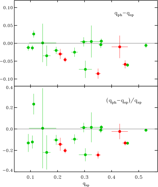
Figure 8: The mass-ratio discrepancy between the photometric, $q_{\rm ph}$, and spectroscopic, $q_{\rm sp}$, determinations is shown directly versus the spectroscopic value (the upper panel) and normalized by $q_{\rm sp}$ (the lower panel). The data shown in green correspond to $q_{\rm sp}$ determinations from the DDO survey while those in red are critically updated spectroscopic results listed by Niarchos & Duerbeck (1991). See the text for details.

Certain precautions were applied to ensure the mutual independence of the $q_{\rm sp}$ and $q_{\rm ph}$ determinations. The selection included only: (1) W UMa-type binaries with $q_{\rm ph}$ Lucy-model determinations published before the spectroscopic determinations, and (2) binaries showing total eclipses to ensure the highest photometric solution stability. The first condition aimed to prevent a “leak” and stabilization of the photometric, iterative, multi-parameter solution on the already available spectroscopic value. The selected binaries are listed in Table 4 which is similar to Table 2 in Niarchos & Duerbeck (1991).

The binaries with $q_{\rm sp}$ from the DDO program are marked in green in Figure 8 and listed in the first half of the table. We added binaries fulfilling the above restrictions from other sources, including the Niarchos & Duerbeck (1991) list, but only those with $q_{\rm sp}$ values determined using the CCF or BF deconvolution methods by other researchers. These results are listed in the second half of Table 4 and are marked by red symbols in the figure. Note that $\epsilon\,$CrA is not included in the table since its primary eclipse may be partial, not total.

The difference $q_{\rm ph}-q_{\rm sp}$ is shown in Figure 8 directly and, similarly as in Niarchos & Duerbeck (1991), in the relative sense, divided by the value of $q_{\rm sp}$. The normalization may artificially amplify discrepancies at the low-end of the mass ratio. Regardless of the presentation, we observe a widespread occurrence of $q_{\rm ph}<q_{\rm sp}$, exactly as for AW UMa, which is the binary with the smallest $q_{\rm sp}$ in the figure. The size of the discrepancy is moderate, so either $q_{\rm sp}$ or $q_{\rm ph}$ could serve as an argument in the figure. However, we believe that the spectroscopic $q_{\rm sp}$ is currently the better-determined value because of its more astrophysically meaningful and straightforward derivation; we return to this subject in Section 7.

The only binary in Figure 8 showing the photometric value of $q_{\rm ph}$ larger than the spectroscopic $q_{\rm sp}$ is FG Hya. This binary has an extensive and consistent record of several photometric determinations, so it urgently requires a confirmation of the spectroscopic result. We note the spectroscopic result was obtained at the very beginning of the DDO program (Lu & Rucinski, 1999).

The study of Niarchos & Duerbeck (1991) presented another strong indication that $q_{\rm ph}$ may be affected by phenomena occurring within the binary system, potentially affecting the applicability of the photometric Lucy model. The authors were confronted with excellent light curves of AE Phe that displayed significant season-to-season changes. One light curve showed a very well-defined total occultation eclipse, while the other light curves showed partial eclipses, usually associated with extensive out-of-eclipse light curve variability. This transition from the total to the partial eclipse already suggests a potential problem with the common-equipotential model for the binary. The authors modelled the four seasonal curves using the Lucy model and found a different $q_{\rm ph}$ for each season, with the range from $0.3836\pm 0.0014$ to $0.3964\pm 0.0010$. Although the formal uncertainties were small, as is almost always the case with the Lucy model solutions, a difference of more than 0.01 between individual determinations of $q_{\rm ph}$ is highly concerning. Strictly speaking, it would imply a large and rapid mass exchange between the components reaching $0.01\,M_{\odot}$ – but without an associated significant orbital-period jump. The Stȩpień model (Section 7.2) can explain the switches from the rounded to the flat-bottomed occultation eclipses in AE Phe as caused by variations in the overall loading of the flow around the secondary component. Unfortunately, no reliable $q_{\rm sp}$ determination is available for that star at this moment.

6 The photometric and spectroscopic mass-ratio determinations

The tendency for $q_{\rm ph}<q_{\rm sp}$ is an important indication that either the Lucy model gives systematically incorrect results for $q_{\rm ph}$ or that the spectroscopic derivations of $q_{\rm sp}$ carry systematic errors. We discuss the new model for W UMa binaries by Stȩpień (2009) in the next Section 7. The model is more complex than the Lucy model and requires the abandonment of the photometric determination of $q_{\rm ph}$.

The one-to-one dependence of the Roche geometry on the mass ratio is the essential property of the Lucy model and the basis for its widespread success in light-curve synthesis codes. The dependence of the radius ratio, $r_{2}/r_{1}$, on the mass ratio, $q=M_{2}/M_{1}$, is a strict relation for an equipotential surface selected to represent the common envelope of the binary. We suggest that this assumption (1) very likely leads to larger uncertainties in $q_{\rm ph}$ than claimed, and (2) may be an indication that the $q_{\rm ph}$ vs. $q_{\rm sp}$ discrepancy points to the failure of the Lucy model.

Determination of the photometric parameters of a W UMa-type binary is a complex process: First, a $3D\rightarrow 1D$ mapping of the stellar brightness (but not velocities) is done for us by the revolving binary. It is registered as a light curve, which is in turn subject to a multi-parameter solution utilizing the Roche-model geometry, with the added Lucy-model prescriptions for handling of stellar-atmosphere properties. The solution is a highly non-linear, iterative process which includes unknowns such as the degree of contact (or the actual value of the common equipotential), and the orbital inclination, intermixed with assumed quantities such as atmospheric properties, such as the local flux level estimated by the limb and gravity darkening laws. Because of the inherent nonlinearities, the parameter determination process is highly prone to biased estimates and may result in deceptively small uncertainties when estimated as for a linear, correlation-free problem. This unfortunately may lead to popularly quoted, but suspiciously small formal uncertainties.

The quoted errors of $q_{\rm ph}$ determinations may in fact be underestimated and may contribute to the observed $q_{\rm ph}$ vs. $q_{\rm sp}$ discrepancy. As an illustration of a prevailing nonlinearity, let’s consider the $r=r(q)$ relation which is essential for the $q_{\rm ph}$ determination. The eclipse effects carry relatively more information than the strongly model-dependent stellar-distortion effects. For spherical stars, it is known that the radius ratio, $k=r_{2}/r_{1}$ (Russell, 1912) is the essential parameter controlling the depth and shape of an eclipsing binary light curve. While in our case the binary components are not spherical stars, an equivalent of $k$ is present, although hidden in light-curve-synthesis code complexities. Individual dimensions of common-equipotential Roche lobes, expressed eg. as side equatorial radii $r_{1}$ and $r_{2}$, depend only on the mass ratio, $r=r(q)$. This relation is known to be non-linear: A simplified version of it has been extensively used by practitioners of close-binary evolutionary calculations to estimate the size of the Roche-lobe (inner critical equipotential) filling component. In the orbital separation units, $r=0.38+0.2\log(q)$; the equation works for both components (with inverted $q$) and has an asymptotic low mass-ratio extension (Paczyński, 1971, Eq.4). We see that, by being approximately logarithmic, the dependence $r=r(q)$ is a slowly-varying function with the Roche-lobe radii are weakly dependent on $q$. It is a convenience for stellar binary models. But the $q_{\rm ph}$ determination utilizes an inverse relation which – consequently – is a rapidly varying function. For the above approximation, it is an exponential function, $q=10^{5r-1.9}$. Therefore, small errors in the relative radius determination produce large deviations in the estimated mass ratio.

The above relations concern a single critical Roche-model lobe. For the ratio of their radii, $k=r_{2}/r_{1}$, the exponential character is partially reduced and the non-linearity is milder. Using the same approximation for the inner critical Roche lobe as above, an approximate relation for the whole range $0<k<1$ is still nonlinear, $q\simeq k^{+2.23\pm 0.03}$. Of course, one may hope that all similar imperfections will somehow average out; we do not see any obvious reason for the occurrence of the $q_{\rm ph}$ vs. $q_{\rm sp}$ discrepancy. The main point remains, that the commonly used linear estimates of uncertainties should be replaced by (probably much larger) estimates obtained using more rigorous statistical methods.

We note that systematically too small values of $q_{\rm ph}$ may result from the presence of an unrecognized “third light” in the light curve. Companions to W UMa binaries are very common (Rucinski et al., 2007). A light curve containing additional light has a reduced amplitude and most likely will give a smaller value of $q_{\rm ph}$. This was exactly the case for the photometric solution for $\epsilon\,$CrA by Shobbrook & Zola (2006), who commented that they had to reduce $q_{\rm ph}$ from the spectroscopic, initially assumed value of $q_{\rm sp}=0.129$ (Goecking & Duerbeck, 1993) by 0.02 to obtain the best fit.

The spectroscopic time-monitoring offers an entirely different and independent route of the mass ratio determination involving a $3D\rightarrow 2D$ mapping, from the spatial velocities into a series of RV profiles arranged in time. This approach ensures that more information is available and in two accessible dimensions of time and radial velocity. The RV dimension is that of the orbital semi-amplitudes $K_{1}$ and $K_{2}$ so that $q_{\rm sp}=K_{1}/K_{2}$. For very tight orbits, as observed for the W UMa-type binaries, with strongly dissipative, gaseous bodies involved, the only permitted orbits are circular, so that the derivation of the semi-amplitudes is particularly simple and direct. Thus – in principle – the spectroscopic $q_{\rm sp}$ is obtained with a lesser danger of biased results. Here, the uncertainties relate to the proper localization of the RV centroids and their coincidence with the projected mass centers. Our results for AW UMa and $\epsilon\,$CrA in P1 and P2 show that the inter-binary velocity fields are present with velocities reaching perhaps as much as 20 – 30 km s^-1. It is not clear if these fields are centered on the projected mass centers. While the rotational-profile centroids seem to work well for the primary components of both binaries, the confined extent of secondaries in velocities (as on detached components) is an unexpected discovery. Are centroids of these very faint features tracing the motion of the secondary components?

7 The W UMa-type binary model

7.1 The Lucy model

When it appeared more than half a century ago, the Lucy (1968a, b) model was the first consistent description of W UMa binaries as dynamically stable configurations of solar-type stars in strong physical contact. The Lucy publication left important structural and energy-related issues open, but the light-curve calculation prescription was very convincing and simple: it suggested that common equipotentials of the Roche binary model as better described W UMa binaries than complex descriptions of large tidal distortions imposed on spherical stars. While the unprecedented idea of two different-mass stars touching each other – and still in equilibrium – was not accepted immediately, the model found enthusiastic approval among binary-star observers interpreting light curves. The model perfectly reproduced the observed light curves, assuming that both stars had identical effective temperatures. The particularly successful work on totally eclipsing W UMa-type binaries by Mochnacki & Doughty (1972a, b) followed by similar investigations by Lucy (1973) and Wilson & Devinney (1973) showed the great potential in that domain. The Lucy prescription found widespread use when ready-made, easy-to-install codes became widely available thanks to the generosity of several investigators (Wilson & Van Hamme, 2009; Prša et al., 2016; Wilson et al., 2020; Conroy et al., 2020). There were voices of a rather low information content of the light curves (Rucinski, 1993, 2001) and of a sensitivity to the ubiquitous presence of third stars (Rucinski et al., 2007), but they were ignored.

Interpretation of the W UMa-type binary light curves unambiguously shows that the effective temperatures of both components are almost perfectly the same, despite commonly observed mass ratios different from unity, sometimes as small as $q\simeq 0.1$, as for our stars or smaller (Wadhwa et al., 2021; Li et al., 2022; Guo et al., 2023). For Main Sequence stars, the ratio of nuclear luminosities scales as $L_{2}/L_{1}\propto q^{\alpha}$ with $\alpha\simeq 4-5$ so that the secondary components in most cases would be expected to be energetically inert stars. To explain the observed equal-temperature property, Lucy (1968a) proposed the turbulent, gravity-driven convection – known for its high efficiency in solar-type stars – as a process carrying energy from the primary to the secondary component. This assumption was entirely ad hoc and most likely incorrect: the force driving convection is directed perpendicularly to the direction of energy transport in the volume between the two stars; therefore, turbulent convection is expected to be entirely extinguished there or to carry insignificant amounts of energy. A more likely seemed to be an organized flow deep in the stellar interior as suggested by Webbink (1976, 1977); however, existing descriptions still did not include the ever-present Coriolis force. In both mechanisms, by Lucy and by Webbink, an assumption was made of energy transport originating in the primary component core and depositing the energy deep inside the secondary. Thus, both can be called the “internal” energy-transport solutions.

An “external” process was proposed by Shu et al. (1976). The authors pointed out that the faster evolutionary expansion of the more massive component may lead to a “boiling over” of the primary-component matter onto the secondary, resulting in a complete enshrouding of the secondary component by the hotter gas. The same matter would then be visible over the whole binary surface. This would perfectly explain the observed temperature equality, but – contrary to normal conditions in external layers of stars – the hot material would have to stably stay on the cooler gas of the secondary. The inverted-temperature solution was strongly criticized as containing deep physical problems and has been abandoned (Papaloizou & Pringle, 1979; Shu et al., 1979).

Since then, for another thirty or so years, research on the internal energetics of the W UMa binaries stagnated, even as the Lucy model continued to perform excellently in reproducing light curves. The Lucy model slowly acquired general acceptance and the unresolved issue of energy transfer ceased to be discussed. The only voice highlighting the lack of any new theoretical research was that of Webbink (2003), but this did not lead to any obvious consequences.

7.2 The Stȩpień model

The Stȩpień (2009) model of W UMa-type binaries focuses on a matter ignored in the Lucy model, specifically the solution of the energy flow between the components. It predicts inter-binary velocities, thereby undermining the main assumption of the Roche geometry, which is the core of the Lucy model. Such velocities have been observed in both binaries discussed in this paper. Both, the observations and the model suggest that the velocities are moderate, allowing the Lucy model and its photometric solutions to continue providing reasonable guidance for the selecting particularly important objects.

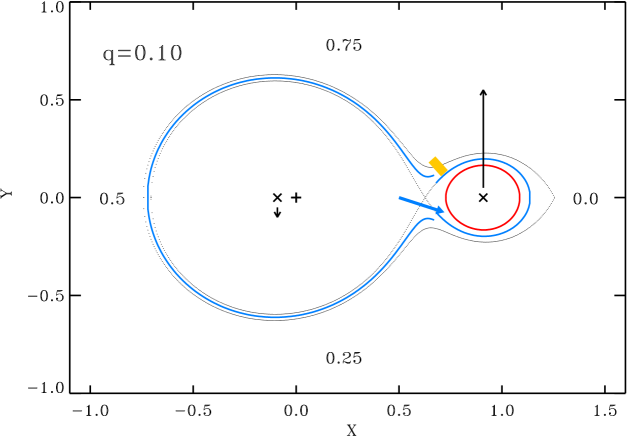
Figure 9: Properties of the Stȩpień (2009) model follow consideration of the initial stages of the Roche-lobe overflow by the primary. The flow is deflected by the Coriolis force to the side of the secondary, building up a thick belt. The shape of the belt in the orbital plane may be close to an equipotential but different from that describing the primary component and very likely tighter. As a result, one component slightly overfills and the other slightly underfills the common equipotential. The figure is for $q=0.10$, similar to that of AW UMa and $\epsilon\,$CrA. The blue line shows the hot gas of the expanding primary, while the secondary component is shown in red. The approximate location of the prominent Enhanced Spectral-line Perturbation (ESP) observed in both binaries is marked in orange. The numbers at the perimeter give the orbital phase positions of an external observer. The arrows at the mass centers represent (in scale) the orbital velocities of the component stars.

As a starting point, the Stȩpień (2009) model utilizes results from detailed hydrodynamical calculations by Oka et al. (2002), who analyzed the velocity field on a Roche-lobe-overflowing component in a close binary system. The other component of the Oka et al. model was an unspecified collapsed star, similar to those in cataclysmic variables, novae, etc. Upon leaving the primary, the gas flow – starting with moderately supersonic velocities – is deflected by the Coriolis force to the side of the secondary. This binary side corresponds to that visible at $\phi=0.25$ in AW UMa and $\epsilon\,$CrA (Figure 9). The analogy with the cataclysmic variables modeled by Oka et al. (2002) ends at this point for W UMa binaries: The flow does not continue into a deep potential well and does not accelerate by falling inwards. Instead, it encounters the outer layers of the secondary component, retaining its original, moderate outflow velocity. The photospheric sound velocity for F-type stars, such as the AW UMa and $\epsilon\,$CrA primaries, is expected to be of the order 7 km s^-1. Thus, the flow would not exceed local velocities of about 10 – 20 km s^-1.

As the matter is continuously transferred, an optically thick belt of hot, primary-component material accumulates in the equatorial region of the secondary. Most of the material makes only a single revolution around the secondary and strikes the primary atmosphere on the side visible in the $\phi=0.75$ hemisphere. This is exactly where we see the strong Enhanced Spectral-line Perturbation (ESP); it is visible in both binaries discussed in this paper, projecting against the secondary profile at the sub-observer phase $\phi\simeq 0.65$ (marked in orange in Figure 9). The net mass transfer between the binary components is minimal, in agreement with the observed, moderate period changes. The flow may continue around the primary component and – with the new matter from the primary – be visible as the “pedestal” of the primary-component profile (item 1. in the list in Section 2). Such a general circulation, when observed in the equatorial plane, could very well assure a light curve typical for a W UMa binary. The energy transfer would be thus similar to the “external” energy-transfer model of the enshrouded secondary (Section 7.1), but (1) only over the equatorial region, and (2) by a slowly moving flow, not by a static, fully-covering shroud. It is possible that cooler, polar regions of the secondary would be visible at larger inclinations, but not necessarily so. As pointed by Stȩpień (2009), a “bottling-up” effect of the secondary component’s own generated energy through the constriction of the hot gas may lead to substantial heating of the polar regions of the secondary.

Will the equatorial flow from the primary component follow the zero-velocity, equipotential surface and mimic the Lucy model? The hot material is injected into the secondary component’s critical lobe at relatively low velocities compared with those involved in the restoration of the dynamical equilibrium in the binary. Thus, the gas may approximately follow an equipotential, but the flow would be subject to energy and angular-momentum losses due to very strong tides. These forces should extract the kinetic energy of the flow and send the material “down”, closer to the surface of the secondary component. Thus, the Stȩpień model offers an interesting prediction which we seem to see demonstrated in the mass-ratio discrepancy (Section 5): On average, we expect that the primary component to slightly exceed the inner critical-lobe dimensions for the given mass ratio, while the transferred matter is injected into the secondary critical equipotential, possibly ending at a surface of smaller dimensions (see Figure 9). This would perfectly agree with the $q_{\rm ph}$ vs. $q_{\rm sp}$ discrepancy: The light-curve solution based on the Lucy model will indicate a systematically smaller mass ratio than the real one, as inferred by a systematically smaller ratio of the radii. Depending on the buildup of the circulation flow, the values of the perceived radii and thus of $q_{\rm ph}$ may change as the flow around the secondary component is loaded by a new matter from the primary. This may explain the mysterious case of the variable $q_{\rm ph}$ in AE Phe, as described by Niarchos & Duerbeck (1991).

The “poor thermal contact binaries” (i.e. binaries as close as those of the W UMa-type, yet with components of unequal temperatures) may be particularly useful in testing details and limits of the Stȩpień model. Siwak et al. (2010) conducted a combined photometric/spectroscopic investigation of several of such binaries utilizing the best currently available techniques. The spectroscopic data show well-defined profiles of cool and faint secondary components and the presence of strong ESP features visible on the $\phi=0.75$ hemisphere. CX Vir was most extensively observed: The “phase 0.65” ESP feature in that binary does not seem to look the same as in AW UMa and $\epsilon\,$CrA; it is much stronger and seems to show a different phase-drift dependence. Firm conclusions from the data in the paper are hard to derive because the available phase coverage is limited to narrow intervals around the orbital quadratures. We can recognize the features interpretable by the Stȩpień model, but the details seem to be different. The poor thermal contact binaries may hold important clues for our understanding of the energy and mass exchange in very close binaries.

8 Conclusions

The paper contains a combined discussion of the previously obtained results for the two W UMa-type binaries, AW UMa (P1) and $\epsilon\,$CrA (P2). Both binaries were subject to time monitoring at a high spectral resolution, and they share many physical properties, notably the very small mass ratio and early-F spectral type. Their similarity resulted mainly from the availability of instrumentation, yet it has revealed interesting and unexpected details discussed in this paper. Also, the later analysis of $\epsilon\,$CrA, which is a simpler binary, helped to interpret unexplained features observed in AW UMa. Both binaries – particularly AW UMa – have been repeatedly observed photometrically, and their light curves perfectly agree with the common-equipotential light-curve-synthesis model of Lucy (1968a, b). However, the spectroscopic view shows a more complex picture: the binaries are not rotating as solid bodies, as required by the strict Lucy model, but they show several phenomena which are related to circumbinary flow with velocities not exceeding 20 – 30 km s^-1. Velocities of that order are predicted in the Stȩpień (2009) model of W UMa binaries, in which the energy transport between the binary components is envisaged as an optically thick belt of the matter originated from the Roche-lobe overfilling primary component (Section 7.2). It remains to be investigated if such relatively moderate velocities, relative to the free-fall or orbital velocities of about 300 km s^-1, invalidate the application of the Lucy model to photometric solutions.

A significant result of this paper is the confirmation of the “large” value of the spectroscopically determined mass-ratio of AW UMa of $q_{\rm sp}=0.092\pm 0.007$ (Section 4), in contrast to the often quoted photometrically derived value, $q_{\rm ph}=0.080\pm 0.005$ (this error from multiple, independent solutions). The new determination agrees with the previous spectroscopic result obtained at a medium spectral resolution, $q_{\rm sp}=0.101\pm 0.006$ (Pribulla & Rucinski, 2008). The difference in spectral resolutions is important as it relates to the different ways of measuring the secondary component RV semi-amplitude $K_{2}$. The new, high spectral resolution result is based on the very weak, almost flat profiles of the AW UMa secondary, disregarding the Enhanced Spectral-line Perturbation (ESP) features; in contrast, the previous medium-resolution measurements included the then unrecognized ESPs in the averaged secondary profiles. The AW UMa secondary shows typically two to four such localized ESPs, which are seen migrating as the binary rotates, in projection onto the secondary profile. In both binaries, one strong ESP was localized in the region between the stars, projecting on the secondary component profile at the sub-observer orbital phase $\phi=0.65$. Such location is expected in the Stȩpień model as a place where the returning stream collides with the primary component after revolving around the secondary.

The tendency for several ESPs in AW UMa does not have an explanation. Being less stable than the single, persistent ESP visible in $\epsilon\,$CrA, they showed a tendency to evolve within hours. Their variability may indicate that the flow around the AW UMa secondary envisaged in the Stȩpień model is more erratic or subject to a pileup than that in $\epsilon\,$CrA. We note the opposite tendencies in the systematic orbital-period changes of the two binaries (Section 2): As indicated by the sign of the period changes, the net mass exchange between the components of AW UMa appears to be directed from the more-massive primary to the less-massive secondary, while it is in the opposite direction in $\epsilon\,$CrA. We may speculate that the multitude of ESPs on the AW UMa secondary signals some sort of “overload” of the flow by the abundance of the incoming matter at this particular stage of binary evolution.

The confirmation of the $q_{\rm ph}<q_{\rm sp}$ inequality in AW UMa, along with the absence (or small size) of a similar discrepancy in $\epsilon\,$CrA, prompted an analysis for several binaries in Section 5. A careful selection of W UMa binaries with spectroscopic $q_{\rm sp}$ determinations and best-constrained Lucy-model solutions indicates that discrepant results are common and that smaller values of $q_{\rm ph}$ are a persistent tendency (Section 5, Figure 8). This could be explained within the Stȩpień (2009) model as due to the tight circulation of the energy-transporting belt around the secondary component in contrast to the expanding, Roche-lobe overfilling primary. Thus, the two stars are expected to show opposite tendencies for deviations from the common equipotential of the Lucy model; this, in turn, could lead to a smaller value of $q_{\rm ph}$ than the real one.

By explaining the energy-transfer problem in the W UMa-type binaries and giving reasons for the $q_{\rm ph}<q_{\rm sp}$ tendency, the Stȩpień model casts a deep shadow on the applicability of the common-equipotential Lucy model for the derivation of physical data for these binaries. Yet, the new model does not bring any predictions on the size of the deviations from the Lucy model nor on ways how to correct its $q_{\rm ph}$ results. Are the results already obtained with the photometric Lucy model still of use? This question applies to large-scale projects utilizing state-of-the-art light-curve synthesis codes (Prša et al., 2016; Conroy et al., 2020; Wilson et al., 2020) to the currently ongoing large photometric surveys, in the spirit of the first explorations based on ASAS (Pilecki, 2009) and OGLE (Soszyński et al., 2015) surveys. A convenient tool for handling statistical $q_{\rm ph}$ data has already been developed by Pešta & Pejcha (2023). Another question is: Are summaries utilizing mixed $q_{\rm ph}$ and $q_{\rm sp}$ data, such as those by Gazeas & Stȩpień (2008) or Gazeas (2024), giving us an unbiased picture?

Concerning further research: The most needed are spectroscopic observations of fainter W UMa-type binaries. The case of AW UMa suggests that medium-resolution ($R\simeq 15,\!000-20,\!000$) data may be adequate for an acceptable determination of $q_{\rm sp}$, but that analysis of detailed profiles and detection of ESPs require a higher resolution ($R>30,\!000$). The binary FG Hya ($V\simeq 10$) is the only case of the inverted mass-ratio discrepancy (Section 5, Figure 8); it urgently requires a new $q_{\rm sp}$ determination. Binaries with less extreme mass ratios particularly need spectroscopic work: We already have tantalizing indications (Pribulla et al., 2006; Pribulla & Rucinski, 2008) that medium-resolution RV profiles for V566 Oph ($V\simeq 7.5$, $q_{\rm sp}=0.263\pm 0.012$) look – unlike those of our two binaries – as predicted by the Lucy model. Interpreted within the Stȩpień model, this may be an indication that the circumbinary flow fully dominates the profile shape. This case possibly sends a signal that by considering our two, extremely low mass-ratio systems, we fortuitously selected atypical binaries with particularly prominent primaries. It may be of use to note that the two binaries considered here may not be the most extreme cases in terms of the very small mass ratio: Smaller values of $q_{\rm ph}$ were already reported in the literature (Wadhwa et al., 2021; Li et al., 2022; Guo et al., 2023).

Two moderately bright W UMa binaries with large mass ratios would be particularly important for further high spectral resolution studies: SW Lac ($V\simeq 8.7$) with $q_{\rm sp}=0.776\pm 0.012$ (Rucinski et al., 2005) and OO Aql ($V\simeq 9.5$) with $q_{\rm sp}=0.846\pm 0.007$ (Pribulla et al., 2007). We noticed during the DDO program that the RV profiles of SW Lac have shapes very much like those of a semi-detached system, yet with components having identical atmospheric properties. Finally, the poor thermal contact binaries, particularly the bright ones previously analyzed by Siwak et al. (2010), may – when observed spectroscopically over all orbital phases – show more details of the flow that in this case is too weak to engulf the equatorial regions of the secondary yet strong enough to produce prominent ESP features.

Theoretical research should elucidate the role of the tidal forces and their dissipation within the circumbinary flow. The results could find application in a full hydrodynamic model of contact systems in the spirit of that of Oka et al. (2002). Such a model could predict the expected velocity profiles in relation to the projected mass centers and help in resolving the matter of the profile centroids used to determine the orbital RV semi-amplitudes.

References

- Anderson et al. (1983) Anderson, L., Stanford, D., & Leininger, D. 1983, ApJ, 270, 200
- Conroy et al. (2020) Conroy, K. E., Kochoska, A., Hey, D., Pablo, H., et al. 2020, ApJS, 250, 34
- Duerbeck (1978) Duerbeck, H. W. 1978, Acta Astr., 28, 49
- Duerbeck & Rucinski (2006) Rucinski, S. M. & Duerbeck, H. W. 2006, AJ, 132, 1539
- Gaia Collaboration (2020) Gaia Collaboration EDR3, 2020, A&A, 649A, 1
- Gazeas (2024) Gazeas, K. 2024, Contr. Astr. Obs. Skalnaté Pleaso, 54, 58
- Gazeas & Stȩpień (2008) Gazeas, K. & Stȩpień, K. 2008, MNRAS, 390, 1577
- Goecking & Duerbeck (1993) Goecking, K.D., & Duerbeck, H.W. 1993, A&A, 278, 463
- Guo et al. (2023) Guo, D.-F., Li, K., Liu, F., Li, H.-Z., & Liu, X.-Y. 2023, MNRAS, 521, 51
- Hilditch & King (1986) Hilditch, R. W. & King, D. J. 1986, MNRAS, 223, 581
- Hill (1979) Hill, G. 1979, Publ. DAO, 15, 297
- Hiller et al. (2004) Hiller, M. E., Osborn, W., & Terrell, D. 2004, PASP, 116, 337
- King & Hilditch (1984) King, D. J. & Hilditch, R. W. 1984, MNRAS, 209, 645
- Lapasset (1980) Lapasset, E. 1980, AJ, 85, 1098
- Leung et al. (1985) Leung, K.-C., Zhai, D., & Zhang, Y. 1985, AJ, 90, 515
- Li et al. (2022) Li, K., Gao, X., Liu, X.-Y., Gao, X. et al. 2022, AJ, 164, 202
- Lu & Rucinski (1999) Lu, W. & Rucinski, S. M. AJ, 118, 515
- Lucy (1968a) Lucy, L. B. 1968a, ApJ, 151, 1123
- Lucy (1968b) Lucy, L. B. 1968b, ApJ, 153, 877
- Lucy (1973) Lucy, L. B. 1973, Ap&SS, 22, 381
- McLean (1981) McLean, B. J. 1981, MNRAS, 195, 931
- McLean & Hilditch (1983) McLean, B. J. & Hilditch, R. W. 1983, MNRAS, 203, 1
- Mochnacki & Doughty (1972a) Mochnacki S.W., & Doughty N.A. 1972a, MNRAS, 156, 51
- Mochnacki & Doughty (1972b) Mochnacki S.W., & Doughty N.A. 1972b, MNRAS, 156, 243
- Niarchos & Duerbeck (1991) Niarchos, P. G. & Duerbeck, H. W. 1991, A&A, 247, 399
- Oka et al. (2002) Oka, K., Nagae, T., Matsuda, T., Fujiwara, H., & Boffin, H. M. J. 2002, A&A, 394, 115
- Paczyński (1964) Paczyński B. 1964, AJ, 69, 124
- Paczyński (1971) Paczyński B. 1964, ARA&A, 9, 183
- Paczyński et al. (2007) Paczyński B., Sienkiewicz, R., & Szczygieł, D. M. 2007, MNRAS, 378, 961
- Papaloizou & Pringle (1979) Papaloizou, J. & Pringle, J. E. 1979, MNRAS, 189, 5P
- Pešta & Pejcha (2023) Pešta, M & Pejcha, O. 2023, A&A, 672, A176
- Pilecki (2009) Pilecki, B. 2009, PhD Thesis, Warsaw University (unpublished)
- Plewa et al. (1991) Plewa, T., Haber, G., Włodarczyk, K. J., & Krzesiński, J. 1991, Acta Ast., 41, 291
- Pribulla & Rucinski (2008) Pribulla, T., & Rucinski, S. M. 2008, MNRAS, 386, 377
- Pribulla et al. (2005) Pribulla, T., Vaňko, M., Chochol, D., Parimucha, Š., & Baluďansky, D. 2005, Ap&SS, 296, 281
- Pribulla et al. (2006) Pribulla, T., Rucinski S. M., Lu, W., Mochnacki, S. W., et al. 2006, AJ, 132, 769
- Pribulla et al. (2007) Pribulla, T., Rucinski S. M., Conidis, G., DeBond, H., et al. 2007, AJ, 133, 1977
- Pribulla et al. (2007) Pribulla, T., Rucinski S. M., Blake, R. M., Lu, W., et al. 2009, AJ, 137, 3655
- Prša et al. (2016) Prša, A., Conroy, K. E., Horvat, M., Pablo, H., et al. 2016, ApJS, 227, 29.
- Rensing et al. (1985) Rensing, M. J., Mochnacki, S. W., & Bolton, C. T. 1985, AJ, 90, 767
- Rieutord et al. (2023) Rieutord, M., Petot, P., Reese, D., Böhm, T., Ariste, A. L., Mirouh, G. M., de Souza, A. D. 2023, A&A, 669, A99
- Robb (1992) Robb, R. M. 1992, Inf. Bull. Variable Stars, No. 3798
- Rucinski (1976) Rucinski S. M. 1976, PASP, 88, 777
- Rucinski (1992) Rucinski S. M. 1992, AJ, 104, 1968
- Rucinski (1993) Rucinski S. M. 1993, PASP, 105, 1433
- Rucinski (2001) Rucinski S. M. 2001, AJ, 122, 1007
- Rucinski (2002a) Rucinski, S. M. 2002a, PASP, 114, 1124
- Rucinski (2002b) Rucinski, S. M. 2002b, AJ, 124, 1746
- Rucinski (2010) Rucinski, S. M. 2010, in Binaries – Key to Comprehension of the Universe, eds. A. Prša, M. Zejda, ASP Conf. Ser. 435, 195
- Rucinski (2012) Rucinski, S. M. 2012, in From Interacting Binaries to Exoplanets: Essential Modeling Tools, eds. M. Richards, & I. Hubeny IAU Symp., 285, 365
- Rucinski (2015) Rucinski S. M. 2015, AJ, 149, 49 (P1)
- Rucinski (2020) Rucinski S. M. 2020, AJ, 160, 104 (P2)
- Rucinski et al. (2007) Rucinski S. M., Pribulla, T., van Kerkwijk, A. H. 2007, AJ, 134, 2353
- Rucinski & Lu (1999) Rucinski, S. M., & Lu, W. 1999, AJ, 118, 2451
- Rucinski et al. (2000) Rucinski, S. M., Lu, W., & Mochnacki, S. W. 2000, AJ, 120, 1133
- Rucinski et al. (2005) Rucinski, S. M., Pych, W., Ogłoza, W., DeBond, H., et al. 2005, AJ, 130, 767
- Rucinski et al. (2008) Rucinski S. M., Pribulla, T., Mochnacki, S. W., Liokumovich, E., et al. 2008, AJ, 136, 586
- Rucinski et al. (2013a) Rucinski, S. M., Pribulla, T., & Budaj, J. 2013a, AJ, 146, 70
- Rucinski et al. (2013b) Rucinski S. M., Matthews, J. M., Cameron, C., Guenther, D. B., et al. 2013b, Inf. Bull. Var. Stars, 6079
- Russell (1912) Russell, H. N. 1912, ApJ, 36, 54
- Samec et al. (1997) Samec, R. G., Pauley, B. R., & Carrigan, B. J. 1997, AJ, 113, 401
- Shobbrook & Zola (2006) Shobbrook, R. R., & Zola, S. 2006, Ap&SS, 304, 43
- Shu et al. (1976) Shu, F. H., Lubow, S. H., & Anderson, L. 1976, ApJ, 209, 536
- Shu et al. (1979) Shu, F. H., Lubow, S. H., & Anderson, L. 1979, ApJ, 229, 223
- Siwak et al. (2010) Siwak, M., Zola, S, & Koziel-Wierzbowska, D. 2010, Acta Astron., 60, 305
- Soszyński et al. (2015) Soszyński, I., Stȩpień, K., Pilecki, B., Mróz, P., et al. 2015, Acta Astron., 65, 39
- Stȩpień (2009) Stȩpień, K. 2009, MNRAS, 397, 857
- Tapia & Whelan (1975) Tapia, S. & Whelan, J., 1975, ApJ, 200, 98
- Twigg (1979) Twigg, L. W. 1979, MNRAS, 189, 907
- Vinkó et al. (1996) Vinkó, J., Hegedüs, T., & Hendry, P. D. 1996, MNRAS, 280, 489
- Wadhwa et al. (2021) Wadhwa, S.S., De Horta, A., Filipović, M.D., Tothill, N. F. H., 2021, MNRAS, 501, 229
- Webbink (1976) Webbink, R. F. 1976, ApJS, 32, 583
- Webbink (1977) Webbink, R. F. 1977, ApJ, 215, 851
- Webbink (2003) Webbink, R. F. 2003, in 3D Stellar Evolution, eds. S. Turcotte, S. C. Keller, R. M. Cavallo, ASP Conf. Series, 293, 76
- Wilson (2008) Wilson, R. E. 2008, ApJ, 672, 575
- Wilson & Raichur (2011) Wilson, R. E., & Raichur, H. 2011, MNRAS, 415, 596
- Wilson & Devinney (1973) Wilson, R. E., & Devinney, E. J. 1973, ApJ, 182, 539
- Wilson & Van Hamme (2009) Wilson, R. E., & Van Hamme, W. 2009, ApJ, 699, 118
- Wilson et al. (2020) Wilson, R. E., Devinney, E. J., & Van Hamme, W. 2020, Astrophysics Source Code Library. ascl:2004.004
- Yang et al. (1991) Yang, Y.-L., Liu, Q.-Y., Zhang, Y.-L., Wang, B., & Lu, L. 1991, Acta Astron. Sinica, 32, 326
- Zhang et al. (1992) Zhang, J. T., Zhang, R. X., & Zhai, D. S. 1992, Acta Astron. Sinica, 33, 131 (Chinese Astron. Astrophys., 16, 407))