$\mu$LO: Compute-Efficient Meta-Generalization of Learned Optimizers

Abstract

Learned optimizers (LOs) can significantly reduce the wall-clock training time of neural networks, substantially reducing training costs. However, they often suffer from poor meta-generalization, especially when training networks larger than those seen during meta-training. To address this, we use the recently proposed Maximal Update Parametrization ($\mu$P), which allows zero-shot generalization of optimizer hyperparameters from smaller to larger models. We extend $\mu$P theory to learned optimizers, treating the meta-training problem as finding the learned optimizer under $\mu$P. Our evaluation shows that LOs meta-trained with $\mu$P substantially improve meta-generalization as compared to LOs trained under standard parametrization (SP). Notably, when applied to large-width models, our best $\mu$LO, trained for 103 GPU-hours, matches or exceeds the performance of VeLO, the largest publicly available learned optimizer, meta-trained with 4000 TPU-months of compute. Moreover, $\mu$LOs demonstrate better generalization than their SP counterparts to deeper networks and to much longer training horizons (25 times longer) than those seen during meta-training.

1 Introduction

Deep learning [13] has enabled a great number of breakthroughs [6, 5, 29, 1, 17, 31, 26]. Its success can, in part, be attributed to its ability to learn effective representations for downstream tasks. Notably, this resulted in the abandonment of a number of heuristics (e.g., hand-designed features in computer vision [11, 21]) in favor of end-to-end learned features. However, one aspect of the modern deep-learning pipeline remains hand-designed: gradient-based optimizers. While popular optimizers such as Adam or SGD provably converge to a local minimum in non-convex settings [16, 19, 30], there is no reason to expect these hand-designed optimizers reach the global optimum at the optimal rate for a given problem. Given the lack of guaranteed optimality and the clear strength of data-driven methods, it is natural to turn towards data-driven solutions for improving the optimization of neural networks.

Existing work [4, 37, 22, 23] has explored replacing hand-designed optimizers with small neural networks called learned optimizers (LOs). [24] showed that scaling up the training of such optimizers has the potential to significantly improve wall-clock training speeds and supersede existing hand-designed optimizers. However, LOs have limitations in generalizing to new problems. For example, despite training for $4000$ TPU months, VeLO [24] is known to (1) generalize poorly to longer optimization problems (e.g., more steps) than those seen during meta-training and (2) have difficulty optimizing models much larger than those seen during meta-training. Given the high cost of meta-training LOs (e.g., when meta-training, a single training example is analogous to training a neural network for many steps), it is essential to be able to train learned optimizers on small tasks and generalize to larger ones. [14] explore preconditioning methods to improve the generalization from shorter to longer optimization problems (e.g., ones with more steps). However, no works focus on improving the generalization of LOs to larger models.

A related problem in the literature is zero-shot hyperparameter transfer, which involves selecting optimal hyperparameters of handcrafted optimizers for training very large networks (that one cannot afford to tune directly) by transferring those tuned on smaller versions of the model. As it was shown in [43], under the standard parametrization (SP), the optimal hyperparameters of an optimizer used for a small model do not generalize well to larger versions of the model. However, [43] demonstrate that when a small model is tuned using the Maximal Update Parametrization ($\mu$P), and its larger counterparts are also initialized with $\mu$P, they share optimal hyperparameters.

Notably, the problem of meta-learning LOs and re-using them on larger unseen architectures can be reformulated as zero-shot hyperparameter transfer. Given this connection between zero-shot hyperparameter transfer and meta-generalization, we ask the following questions: Can learned optimizers be meta-trained under $\mu$P? Would the resulting optimizers benefit from improved generalization? We seek to answer these questions in the following study. Specifically, we consider the popular per-parameter LOs architecture introduced by [23] and demonstrate that $\mu$P can be adapted to this optimizer. We subsequently conduct an empirical evaluation which reveals the power of our $\mu$LO and its large advantages for scaling learned optimizers.

Our contributions can be summarized as follows:

• We demonstrate that $\mu$P can be adapted to the case of per-parameter MLP learned optimizers.

• We empirically demonstrate that $\mu$LOs significantly improve generalization to wider networks as compared to their SP counterparts and that, for the widest models, they outperform VeLO (Meta-trained with 4000 TPU-months of compute).

• We empirically demonstrate that $\mu$LOs significantly improve generalization to longer training horizons (shown for $25\times$ meta-training) as compared to their SP counterparts.

• We empirically demonstrate that $\mu$LOs show improved generalization to deeper networks as compared to their SP counterparts.

Our results show that $\mu$LOs significantly improve learned optimizer generalization without increasing meta-training costs. This constitutes a noteworthy improvement in the scalability of meta-training LOs.

2 Related Work

Learned optimization.

While research on learned optimizers (LOs) spans several decades [32, 34, 10, 3], our work is primarily related to the recent meta-learning approaches utilizing efficient per-parameter optimizer architectures of [23]. Unlike prior work [4, 37, 9], which computes meta-gradients (the gradients of the learned optimizer) using backpropagation, [23] use Persistent Evolutionary Strategies (PES) [36], a truncated variant of evolutionary strategies (ES) [7, 25, 27]. ES improves meta-training of LOs by having more stable meta-gradient estimates compared to backpropagation through time, especially for longer sequences (i.e. long parameter update unrolls inherent in meta-training) [22]. PES and most recently ES-Single [35] are more efficient and accurate variants of ES, among which PES is more well-established in practice making it a favourable approach to meta-training.

Generalization in LOs.

One of the critical issues in LOs is generalization in the three main aspects [10, 3]: (1) optimize novel tasks (which we refer to as meta-generalization); (2) optimize for more iterations than the maximum unroll length used in meta-training; (3) avoid overfitting on the training set. Among these, (3) has been extensively addressed using different approaches, such as meta-training on the validation set objective [22], adding extra-regularization terms [14], parameterizing LOs as hyperparameter controllers [2] and introducing flatness-aware regularizations [44]. The regularization terms [14, 44] often alleviate issue (2) as a byproduct. However, meta-generalization (1) has remained a more difficult problem. One approach to tackle this problem is to meta-train LOs on thousands of tasks [24]. However, this approach is extremely expensive and does not address the issue in a principled way leading to poor meta-generalization in some cases, e.g. when the optimization task includes much larger networks. Alternatively, [28] introduced Loss-Guarded L2O (LGL2O) that switches to Adam/SGD if the LO starts to diverge improving meta-generalization. However, this approach needs tuning Adam/SGD and requires additional computation (e.g. for loss check) limiting (or completely diminishing in some cases) the benefits of the LO. In this work, we study aspects (1) and (2) of LO generalization, demonstrating how existing SP LOs generalize poorly across these dimensions and showing how one can apply $\mu$P to learned optimizers to substantially improve generalization in both these aspects.

Maximal Update Parametrization.

First proposed by [41], the Maximal Update Parametrization is the unique stable abc-Parametrization where every layer learns features. The parametrization was derived for adaptive optimizers in [42] and was applied by [43] to enable zero-shot hyperparameter transfer, constituting the first practical application of the tensor programs series of papers. Earlier works in the tensor programs series build the mathematical foundation that led to the discovery of $\mu$P. [38] shows that many modern neural networks with randomly initialized weights and biases are Gaussian Processes, providing a language, called Netsor, to formalize neural network computations. [39] focuses on neural tangent kernels (NTK), proving that as a randomly initialized network’s width tends to infinity, its NTK converges to a deterministic limit. [40] shows that a randomly initialized network’s pre-activations become independent of its weights when its width tends to infinity. Building on the latest works in the tensor program series,  [42] and [43], in this work, we show that $\mu$P can easily be extended to the case of per-parameter learned optimizers and empirically evaluate its benefits in this setting.

3 Method

3.1 Background

A standard approach to learning optimizers [23] is to solve the following meta-learning problem:

$$\min_{\phi}\;\mathbb{E}_{({\mathcal{D}},{\bm{w}}_{0})\sim{\mathcal{T}}}\;\mathbb{E}_{(X,Y)\sim{\mathcal{D}}}\left(\frac{1}{T}\sum_{t=0}^{T-1}{\mathcal{L}}(X,Y;f_{\phi}(\cdot))\right),$$ (1)

where ${\mathcal{T}}$ is a distribution over optimization tasks defined as pairs of dataset ${\mathcal{D}}$ and initial weights ${\bm{w}}_{0}$ associated with a particular neural architecture (we refer to this network as the optimizee), $\phi$ represents the weights of the learned optimizer, $f_{\phi}$. Finally, ${\mathcal{L}}$ is the loss function used to train the optimizee. $T$ is the length of the unroll which we write as a fixed quantity for simplicity. In our experiments, during meta-optimization, $T$ is varied according to a truncation schedule [23]. A clear goal of the learned optimization community is not only learning to solve optimization problems over ${\mathcal{T}}$, but also to apply the learned optimizer, $f_{\phi}$, more generally to unobserved datasets and architectures. This transfer to new tasks is referred to as meta-generalization. This problem can be seen as a generalization of the zero-shot hyperparameter transfer problem considered in [43]; for instance, when the optimizer is a hand-designed method such as SGD or Adam and $\phi$ represents optimization hyper-parameters such as the learning rate.

Gradient descent is a standard approach to solving equation 1. However, estimating the meta-gradients via backpropagation for very long unrolls is known to be noisy [22]. Instead, gradients are estimated using evolutionary strategies [7, 25, 27]. Evolutionary strategies work by sampling perturbations to the LO’s weights (similar to SPSA [33]), unrolling an optimization trajectory for each perturbation, and estimating gradients with respect to evaluations of the meta-objective (usually the loss of the network being optimized, see eq. 1). In contrast to ES, which estimates one gradient per full unroll, PES [36] allows estimating unbiased gradients at many points (called truncations) during the full unroll. This allows updating the optimizer’s parameters more often during meta-training. We use PES to estimate meta-gradients in our experiments.

Our learned optimizer architectures for $f_{\phi}$ is per-parameter; that is, it is applied once for each parameter in the optimizee. Each parameter’s features are constructed based on momentum, second-order momentum, and adafactor values as in [23], with the full list of features described in the (Table 3 of the Appendix). The architecture of our $f_{\phi}$ is similar to small_fc_lopt of [23], it is a 2-layer MLP with width $32$. $f_{\phi}$ has two outputs $m$ and $d$, the magnitude and scale of the update respectively. The standard LO update is given as

$$w_{t}=w_{t-1}-\lambda_{1}d_{\phi}\exp{\left(\lambda_{2}m_{\phi}\right)},$$ (2)

where $\lambda_{1}$ and $\lambda_{2}$ are constant values of $0.001$ to bias initial step sizes towards being small.

3.2 $\mu$LO

Consider a model to be optimized $g_{w}$ with weights in layers $l$ denoted $w_{l}$. We perform and construct $\mu$LOs as follows.

Initialization-$\mu$.

$w_{l}$ which are hidden and input layers (aka the output sizes that can increase) have their weights initialized as $\mathcal{N}(0,\frac{1}{\sqrt{\textsc{fan\_in}}})$. While output layers (those mapping to fixed sizes) have their weights initialized as $\mathcal{N}(0,1)$.

Multipliers-$\mu$.

Output layers pre-activations are multiplied by $\frac{1}{\textsc{fan\_in}}$ during the forward pass.

Updates-$\mu$.

The update by $f_{\phi}$ on the parameters of $g_{w}$, at both meta-training and evaluation is modified as follows:

$$w_{t}=\begin{cases}w_{t-1}^{i}-\frac{1}{\textsc{fan\_in}}\cdot\left(\lambda_{1}d_{\phi}^{i}\exp{\left(\lambda_{2}m_{\phi}^{i}\right)}\right)&\text{if $w^{i}$ is part of a hidden layer}\\ w_{t-1}^{i}-\lambda_{1}d_{\phi}^{i}\exp{\left(\lambda_{2}m_{\phi}^{i}\right)}&\text{otherwise.}\end{cases}$$ (3)

We now show that this can lead to a maximal update Parametrization, following the analysis of [43, Appendix J.2.1] which studies the initial optimization step. For our analysis, we consider a simplified input set for $f_{\phi}$ which takes as input only the gradient while producing an update for each layer. Note that this analysis extends naturally to other first-order quantities.

Proposition 1.

Assume that the LO $f_{\phi}$ is continuous around 0. Then, if $f_{\phi}(0)\neq 0$, the update, initialization, and pre-activation multiplier above is necessary to obtain a Maximal Update Parametrization.

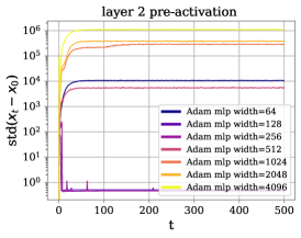
((a))

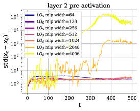
((b))

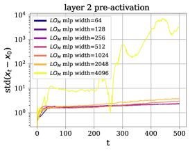
((c))

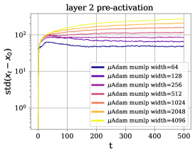
((d))

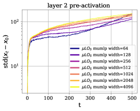
((e))

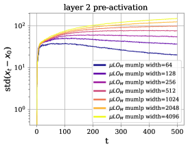
((f))

Figure 1: Pre-activations behave harmoniously in $\mu$P for LOs and Adam alike. We report the evolution of coordinate-wise standard deviation of the difference between the initial ($t=0$) and $t$-th second-layer pre-activations of an MLP during training (the remaining layers behave similarly, see Sec. G). We observe that all models parameterized in $\mu$P enjoy stable coordinates across scales, while the pre-activations of models in SP blow up after a number of training steps.

4 Empirical evaluation

We use a suite of optimization tasks to evaluate meta-generalization properties of our $\mu$LOs vs tuned $\mu$Adam [43] and baseline LOs, including pretrained VeLO [24] (the strongest publicly available pre-trained learned optimizer). We focus on evaluating generalization to wider networks, however, we also verify if $\mu$LOs can improve generalization to longer training horizons and deeper networks.

Table 1: Meta-training configurations of LOs and baselines in our empirical evaluation.

Identifier Type Architecture Optimizee Par. Meta-Training/Tuning Task(s) $\mu\text{LO}_{S}$ Ours small_fc_lopt [23] Adam $\mu$P ImageNet classification, 3-Layer MLP, width $\in\{128\}$ $\mu\text{LO}_{M}$ Ours small_fc_lopt [23] Adam $\mu$P ImageNet classification, 3-Layer MLP, width $\in\{128,512,1024\}$ $\mu$Adam_S Baseline – Adam $\mu$P ImageNet classification, 3-Layer MLP, width $\in\{128\}$ $\mu$Adam_M Baseline – Adam $\mu$P ImageNet classification, 3-Layer MLP, width $\in\{1024\}$ $\text{LO}_{S}$ Baseline small_fc_lopt [23] SP ImageNet classification, 3-Layer MLP, width $\in\{128\}$ $\text{LO}_{M}$ Baseline small_fc_lopt [23] SP ImageNet classification, 3-Layer MLP, width $\in\{128,512,1024\}$ VeLO SOTA Baseline VeLO [24] SP We refer the reader to [24, Appendix C.2]

Baseline LOs and $\mu$LOs. The training configuration of each learned optimizer is summarized in Table 1. Each LO is a 2-layer width $32$ per-parameter MLP [23]. The first baseline optimizer, $\text{LO}_{S}$, is trained on a single task where the optimizee is initialized via SP (standard parametrization as in previous works). This is the single task baseline which we assume to meta-generalize poorly to many tasks in our suite. The second baseline optimizer, $\text{LO}_{M}$, is trained on three versions of the same task where the width of the optimizee MLP changes. This baseline sheds light on whether simply varying the optimizee width during meta-training is enough to achieve generalization of the LO to wider networks. Our $\mu\text{LO}_{S}$ and $\mu\text{LO}_{M}$ are trained on the same tasks as $\text{LO}_{S}$ and $\text{LO}_{M}$, but the optimizee MLPs and parameter updates are parameterized in $\mu$P (section 3.2). For the inner optimization task, we used a maximum unroll length of $1000$ iterations. For all meta-training and hyperparameter tuning details, including their ablation experiments see section D of the appendix.

Pre-trained VeLO. VeLO [24] is a learned optimizer that was meta-trained on a curriculum of progressively more expensive meta-training tasks for a total of $4000$ TPU months. These tasks include but are not limited to image classification with MLPs, ViTs, ConvNets, and ResNets; compression with MLP auto-encoders; generative modeling with VAEs; and language modeling with transformers and recurrent neural networks. During meta-training, VeLO unrolls inner problems for up to 20k steps ($20\times$ ours); the final model was then fine-tuned on tasks with up to 200k steps of optimization. VeLO, therefore, represents the strongest baseline in our empirical evaluation.

Is Pre-trained VeLO a fair baseline? While we believe the comparison is important given the relevance of our results to scaling up LOs, we highlight that the comparison will unfairly advantage VeLO as all tasks in our suite fall within its meta-training distribution and VeLO was meta-trained on inner unroll horizons well beyond those we evaluate. Thus when comparing our LOs to VeLO, it is important to keep in mind that ours are meta-trained with only $0.004\%$ of VeLO’s compute budget.

$\mu$Adam_S and $\mu$Adam_M baselines. We tune two Adam baselines that follow $\mu$P Adam [43] on the same meta-training tasks as our learned optimizers and transfer the hyperparameters to the evaluation tasks making them fair baselines (Table 1). We tune the learning rate and three multipliers: input multiplier, output multiplier, and the hidden learning rate multiplier. These multipliers correspond to adding a tunable constant to the pre-activation multiplier for input weights, the pre-activation multiplier for output weights, and the Adam LR for hidden weights. More details about the grid search over $500$ configurations are provided in Section C of the appendix.

Evaluation tasks. Our evaluation suite includes 20 tasks spanning image classification (CIFAR-10, ImageNet) using MLPs and Vision Transformers (ViTs) [12] and autoregressive language modeling with a decoder-only transformer on LM1B [8]. To create the tasks, we further vary image size (for image classification), width and depth of the optimizee network, and the number of optimization steps. See Table 4 of the appendix for an extended description of all the tasks.

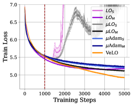
((a))

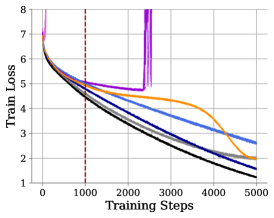
((b))

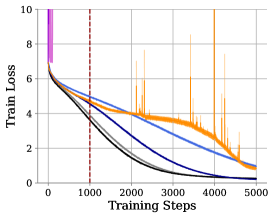
((c))

Figure 2: Evaluating generalization to wider networks. We train MLPs of different sizes to classify $32\times 32\times 3$ ImageNet images. Our optimizers are meta-trained for $1000$ inner steps (dotted red line), therefore, any optimization beyond $1000$ steps is considered out-of-distribution. We observe that $\mu\text{LO}_{M}$ generalize smoothly to all tasks, even surpassing the performance of VeLO (Fig.(b),(c)). We plot average training loss over $5$ seeds with standard error bars.

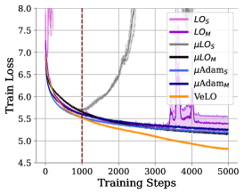
((a))

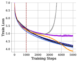
((b))

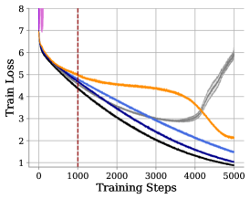
((c))

Figure 3: Meta-generalization to larger images and wider networks. We train MLPs of different sizes to classify $64\times 64\times 3$ ImageNet images. Our optimizers are meta-trained for $1000$ inner steps (dotted red line), therefore, any optimization beyond $1000$ steps is considered out-of-distribution. We observe that $\mu\text{LO}_{M}$ generalizes smoothly to all tasks, obtaining the best performance on the largest task. We plot average training loss over $5$ seeds with standard error bars.

4.1 Results

In the following sections, we first (section 4.1.1) present results empirically verifying the pre-activation stability of our $\mu$LOs and subsequently present the results of our empirical evaluation of meta-generalization to wider networks, deeper networks, and longer training horizons. In section 4.1.2, we start by evaluating our learned optimizers and the corresponding baselines in-distribution and on wider versions of the meta-training task(s) (Figure 2). Continuing with our evaluation of large widths, we study generalization to larger input images (e.g., a wider input layer) and wider hidden layers in Figure 3 and generalization to Cifar-10 (e.g., a smaller output layer) and wider hidden layers in Figure 4. To conclude our study of generalization to larger width, in section 4.1.3, we evaluate our optimizers on out-of-distribution ViT image classification and autoregressive language modeling (figure 5). In section 4.1.4, we transition to evaluating deeper versions of the MLP, ViT, and LM tasks seen previously (see figure 6). Finally, in section 4.1.5, we evaluate generalization to longer unrolls (25$\times$ meta-training) for MLP, ViT, and LM tasks (see figure 7).

4.1.1 Evaluating pre-activation stability

We now verify that desiderata J.1 of [43] is satisfied empirically. In Figure 1, we report the evolution of the coordinate-wise standard deviation of the difference between initial (t=0) and current (t) second-layer pre-activations of an MLP during the first $500$ steps of training. We observe that all models parameterized in $\mu$P enjoy stable coordinates across widths, while the pre-activations of the larger models in SP blow up after a number of training steps. Notably, SP Adam’s pre-activations blow up immediately, while $\text{LO}_{S}$ and $\text{LO}_{M}$ take longer to blow up and have a more erratic pattern; we hypothesize that this is a side effect of meta-training where the optimizers may learn to keep pre-activations small by rescaling updates. Section G of the appendix contains similar plots for the remaining layers of the MLP which show similar trends.

In summary, we find, empirically, that pre-activations of $\mu$LOs and $\mu$Adam are similarly stable across widths, while the activations of SP Adam and SP LOs both blow up but behave qualitatively differently.

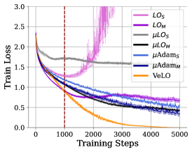
((a))

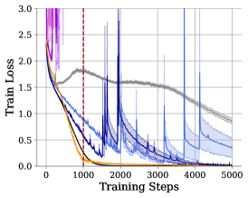
((b))

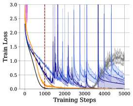
((c))

Figure 4: Meta-generalization to Cifar-10 and wider networks. We train MLPs of different sizes to classify Cifar-10 images. Our optimizers are meta-trained for $1000$ inner steps (dotted red line), therefore, any optimization beyond $1000$ steps is considered out-of-distribution. We observe that $\mu\text{LO}_{M}$ generalizes seamlessly to all tasks, reaching $0$ loss before VeLO in subplots (b) and (c) while all other optimizers struggle to train stably. We plot average training loss over $5$ seeds with standard error bars.

4.1.2 Meta-generalization to wider networks

Wider hidden layers. Figure 2 reports the results for optimizers evaluated on tasks ${\mathcal{T}}^{\text{MLP}}_{1},{\mathcal{T}}^{\text{MLP}}_{3},{\mathcal{T}}^{\text{MLP}}_{4}$, which involve training an MLP of width W=128, W=2048 and W=8192 (at least 8 times wider compared to those used in meta-training). The MLPs are trained on $32\times 32\times 3$ images of ImageNet for $5000$ steps. Since LOs are meta-trained for $1000$ inner steps, steps $1000-5000$ are considered out-of-distribution, posing an additional challenge for meta-generalization. Among the optimizers, $\text{LO}_{S}$ performs the worst diverging after around 1000 steps (Fig. 2, (a)) or immediately (Fig. 2, (b) and (c)). In contrast, our $\mu\text{LO}_{S}$ generalizes seamlessly to the larger tasks matching (Fig. 2, (b)) or improving upon VeLO (Fig. 2, (c)). However, $\mu\text{LO}_{S}$ diverges on the small task (Fig. 2, (a)), which may be caused by slight overfitting on the meta-training task leading to larger updates causing divergence. Compared to $\mu\text{LO}_{S}$, our $\mu\text{LO}_{M}$ generalizes seamlessly without diverging. This generalization is especially notable as its counterpart in SP, $\text{LO}_{M}$, comes nowhere close. Moreover, $\mu\text{LO}_{M}$ beats VeLO (Fig. 2, (b) and (c)) despite VeLO’s massive meta-training budget. While $\mu$Adam also shows strong performance, it underperforms our $\mu\text{LO}_{M}$ in all cases.

Larger images and wider hidden layers. Figure 3 reports the results for LOs evaluated on tasks ${\mathcal{T}}^{\text{MLP}}_{5}$-${\mathcal{T}}^{\text{MLP}}_{7}$, which involve training an MLP of width W=128, W=512 and W=2048 on $64\times 64\times 3$ images of ImageNet. This task evaluates generalization to a wider input layer and, therefore, all tasks are considered out-of-distribution. The $\text{LO}_{S}$ baseline is incapable of generalizing to these tasks, diverging at the beginning in each case. $\text{LO}_{M}$ performs slightly better indicating that meta-training on more tasks helps to some extent, however it still converges poorly for W=128 and W=512 and diverges for W=2048. Unlike $\text{LO}_{S}$, our $\mu\text{LO}_{S}$ only diverges after $1000$ steps of optimization and improves its performance for longer unrolls as the task size increases (similarly to Fig. 2). Once again, $\mu\text{LO}_{M}$ generalizes seamlessly to all tasks without encountering any instabilities outperforming VeLO and other optimizers at W=2048. The $\mu$Adam baselines generalize well to these tasks, however as in previous experiments, they underperform our $\mu\text{LO}_{M}$ overall.

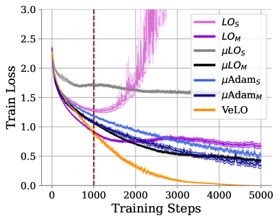
((a))

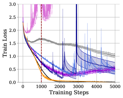
((b))

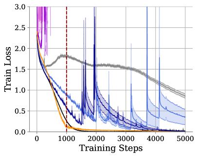
((c))

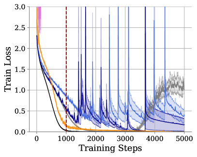
((d))

Figure 10: Meta-generalization to Cifar-10 and wider networks. We train MLPs of different sizes to classify Cifar-10 images. Our optimizers are meta-trained for $1000$ inner steps (dotted red line), therefore, any optimization beyond $1000$ steps is considered out-of-distribution. We observe that $\mu\text{LO}_{M}$ generalizes seamlessly to all tasks, reaching $0$ loss before VeLO in subplots (b),(c),(d) while all other optimizers struggle to train stably. We plot average training loss over $5$ seeds with standard error bars.

CIFAR-10 and wider hidden layers. Figure 4 reports the results of optimizers evaluated on tasks ${\mathcal{T}}^{\text{MLP}}_{8}$,${\mathcal{T}}^{\text{MLP}}_{10}$, and ${\mathcal{T}}^{\text{MLP}}_{11}$ (see ${\mathcal{T}}^{\text{MLP}}_{9}$ results in Fig. 10 of the appendix). Each of these tasks involves training an MLP of different width to classify CIFAR-10 images. These tasks can be seen as evaluating generalization to a smaller output layer size while width is increased. Aligned with our previous experiments, the baseline $\text{LO}_{S}$ and $\text{LO}_{M}$ struggle to generalize either diverging or converging slowly. Our $\mu\text{LO}_{S}$ is more stable, however $\mu\text{LO}_{M}$ is again the best on larger networks monotonically decreasing the loss. Notably, it even reaches loss=0 before VeLO at width W=512,2048,8192. In this case, we observe much superior generalization on the part of $\mu\text{LO}_{M}$ when compared to $\mu$Adam_S and $\mu$Adam_M whose training curves are fraught with instability.

In summary, the results in Fig. 2,3 and 4 indicate that simply meta-training on more tasks is not enough to achieve strong meta-generalization, while $\mu$LO can enable such meta-generalization even outperforming VeLO in some cases.

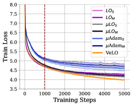
((a))

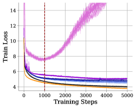
((b))

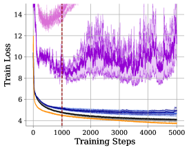
((c))

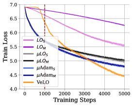
((d))

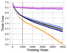
((e))

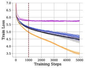
((f))

Figure 5: Meta-generalization to wider out-of-distribution tasks. We report the performance of our optimizers on autoregressive language modeling (top) and ViT image classification (bottom). The datasets used are LM1B and $32\times 32\times 3$ ImageNet, respectively. We observe that $\mu\text{LO}_{S}$ and $\mu\text{LO}_{M}$ train stably and consistently outperform all optimizers except VeLO (LM) our outperform SP LOs and match $\mu$Adam (ViT). We plot average training loss over $5$ seeds with standard error bars.

4.1.3 Meta-generalization far out-of-distribution

In the previous section, some of the tasks were out-of-distribution but remained similar. In this sections, we evaluate on the drastically different tasks than those used to meta-train our optimizers.

Language modeling. We train 3-layer decoder-only transformers of different widths on LM1B for $5000$ steps. The batch size is set to $128$ and the sequence length is set to $64$. Figure 5 (a,b,c) reports the training loss over iterations for each optimizer. We observe smooth training curves for $\mu\text{LO}_{S}$ and $\mu\text{LO}_{M}$ which best all optimizers except VeLO at every width. In contrast, $\text{LO}_{S}$ and $\text{LO}_{M}$ encounter training instabilities at $w=1024,2048$ and $w=2048$ respectively, significantly underperforming $\mu$LOs. While the $\mu$Adam baselines train stably, they underperform $\mu$LOs. Finally, VeLO performs best of all on all tasks which is expected given its compute budget (more than $28,000\times$ the compute used by $\mu\text{LO}_{M}$) and the fact that these tasks (including batch size) fall under its meta-training distribution.

ViT image classification. We train 3-layer ViTs of different widths to classify $32\times 32\times 3$ ImageNet images. The batch size is set to $1024$ . Figure 5 (d,e,f) reports the training loss over iterations for each optimizer. We observe smooth training curves for $\mu\text{LO}_{S}$ and $\mu\text{LO}_{M}$ which best SP LOs at each width and improve on $\mu$Adam as width increases. While $\text{LO}_{S}$ and $\text{LO}_{M}$ do not diverge, for larger models they have difficulty decreasing loss after the first $500$ steps and they significantly underperform $\mu$ LOs across the board. Similarly to the language task, VeLO performs the best as expected.

In summary, even for out-of-distribution tasks, we observe seamless generalization for our $\mu$LOs, showing that using $\mu$P can significantly improve optimizer quality without increasing meta-training time.

4.1.4 Meta-generalization to deeper networks

In this section, we evaluate LO meta-generalization to deeper networks. Specifically, we increase the number of layers used in MLP, ViT, and LM tasks from $3$ to $16$, while being sure to select models that have widths within the meta-training range ($128-1024$) to avoid confounding the results. Figure 6 reports the performance of our multi-task learned optimizers on deeper networks. We observe that $\mu\text{LO}_{M}$ optimizes stably throughout and outperforms $\text{LO}_{M}$ by the end of training on each task, despite being meta-trained on MLPs of exactly the same depth. Moreover, $\text{LO}_{M}$ immediately diverges when optimizing the deep MLP while $\mu\text{LO}_{M}$ experience no instability. This is remarkable as, unlike width, there is no theoretical justification for $\mu$P’s benefit to deeper networks. We hypothesizes that $\mu$P’s stabilizing effect on networks activations leads to this improvement generalization.

In summary, we find, empirically, that using $\mu$P during meta-training benefits the generalization of learned optimizers to deeper networks.

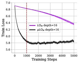
((a))

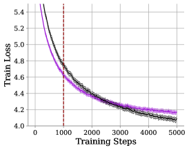
((b))

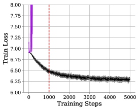
((c))

Figure 6: Evaluating generalization capabilities of $\mu\text{LO}_{S}$ to deeper networks. The figures report the performance of learned optimizers for training depth-16 ViTs for image classification, Transformers for language modeling, and MLPs for image classification. We plot average training loss over $5$ seeds with standard error bars.

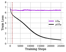
((a))

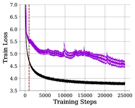
((b))

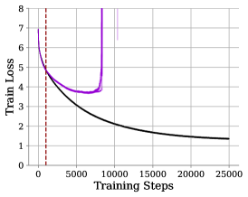
((c))

Figure 7: Evaluating generalization capabilities of $\mu\text{LO}_{S}$ to longer training horizons. $\mu\text{LO}_{S}$ is meta-trained for $1000$ steps of training (dotted red line), therefore, any optimization beyond $1000$ steps is considered out-of-distribution. We observe that the optimizer seamlessly generalizes to training horizons much longer than meta-training (25$\times$ longer, here).

4.1.5 Meta-generalization to longer training horizons

In this subsection, we evaluate the capability of $\mu$LOs to generalize to much longer training horizons than those seen during meta-training. Specifically, we use $\mu\text{LO}_{M}$ and $\text{LO}_{M}$ to train a $w=1024$ 3-layer MLP and ViT on $32\times 32\times 3$ ImageNet and a $w=1024$ 3-layer Transformer for autoregressive language modeling on LM1B. Each model is trained for $25,000$ steps (25$\times$ the longest unroll seen at meta-training time). Figure 7 reports the training loss averaged over $5$ random seeds. We observe that $\mu\text{LO}_{M}$ stably decreases training loss over time for each task, while $\text{LO}_{M}$ fails to decrease training loss (a), decreases it but suffers instabilities (b), or diverges after $8000$ steps (c). These results suggest that generalization to longer training horizons is another benefit of using $\mu$P with learned optimizers.

In summary, we find, empirically, that using $\mu$P during meta-training significantly benefits the generalization of learned optimizers to longer training horizons.

5 Limitations

While we have conducted a systematic empirical study and shown strong results within the scope of our study, there are a number of limitations of our work. Specifically, (1) we do not meta-train on tasks other than MLPs for image classification and we do not provide evaluation of models wider than $8192$ (MLPs) and $2048$ (transformers) due to computational constraints in our academic environment.

6 Conclusion

We have demonstrated that parameterizing networks in $\mu$P significantly improves the generalization of LOs to wider networks than those seen during training, even surpassing VeLO (meta-trained for $4000$ TPU months) on the widest tasks. Moreover, our experiments show that networks trained with $\mu$P generalize better to wider and deeper out-of-distribution tasks than their SP counterparts. When evaluated on much longer training tasks, we observe that $\mu$P has a stabilizing effect, enabling meta-generalization to much longer unrolls ($25\times$ maximum meta-training unroll length). All of the aforementioned benefits of $\mu$LOs come at zero extra computational cost compared to SP LOs. Our results outline a promising path forward for low-cost meta-training of learned optimizers that can generalize to large unseen tasks.

Appendix A Table of Contents

Contents

1. 1 Introduction
2. 2 Related Work
3. 3 Method
   1. 3.1 Background
   2. 3.2 $\mu$LO
4. 4 Empirical evaluation
   1. 4.1 Results
      1. 4.1.1 Evaluating pre-activation stability
      2. 4.1.2 Meta-generalization to wider networks
      3. 4.1.3 Meta-generalization far out-of-distribution
      4. 4.1.4 Meta-generalization to deeper networks
      5. 4.1.5 Meta-generalization to longer training horizons
5. 5 Limitations
6. 6 Conclusion
7. A Table of Contents
8. B Proof of proposition 1
9. C Hyperparameter tuning $\mu$Adam
10. D Meta-training with $\mu$LOs
11. E Features of the learned optimizer
12. F Extended Results
    1. F.1 List of Meta-testing Tasks
    2. F.2 Extended results
13. G Coordinate evolution of MLP layers in $\mu$P for different optimizers

Appendix B Proof of proposition 1

Proposition 1.

Assume that the LO $f_{\phi}$ is continuous around 0. Then, if $f_{\phi}(0)\neq 0$, the update, initialization, and pre-activation multiplier above is necessary to obtain a Maximal Update Parametrization.

Proof.

The update produced by $f_{\phi}$ is denoted $\Delta W$ and we write $\nabla W$ the corresponding gradient, so that $\Delta W=f_{\phi}(\nabla W)$. For the sake of simplicity, $n$ will be the output size and $d$ the feature input size of our neural network. Our goal is to satisfy the desiderata of [43, Appendix J.2]. We assume our initialization follows Initialization-$\mu$ in Sec 3. Overall, our goal is to study strategy so that if $x_{i}=\Theta(1)$, then one needs to renormalize/initialize so that $(Wx)_{i}=\Theta(1)$ while $((W+\Delta W)x)_{i}=\Theta(1)$ so that the update is as large as possible. Note that given the assumptions on $f$, if $x=\Theta(\frac{1}{n})$, then $f(x)=\Theta(1)$.

Output weights.

Here, if input $x$ has some $\Theta(1)$ coordinates, we initialize $W=(w_{i})_{i\leq n}$ with weights of variance 1 (which is necessary) and rescale the preactivations with $\frac{1}{n}$. For the update, we thus have that $\nabla W$ scales (coordinate wise) as $\Theta(\frac{1}{n})$ and we do not rescale the LR, given that $f_{\phi}(\nabla W)$ will also have coordinates in $\Theta(1)$.

Hidden weights.

Now, for the update, we observe that the gradient $\nabla W$ has some coordinates which scale as $\Theta(\frac{1}{n})$, due to the output renormalization choice. Thus, the LO $f_{\phi}(\nabla W)$ satisfies that $f(\nabla W)=\Theta(1)$, given that $f_{\phi}$ is continuous in 0 and satisfies $f_{\phi}(0)\neq 0$. Thus for the update, we need to use $\Delta W=\frac{1}{n}f_{\phi}(\nabla W)$ so that $\Delta Wx$ is coordinate wise bounded.

Input weights.

In this case, the gradient has coordinates which already scale in $\Theta(\frac{1}{n})$ (due to the output renormalization) and there is no need to rescale the LR. ∎

Appendix C Hyperparameter tuning $\mu$Adam

We tune two $\mu$Adam baselines on the same meta-training tasks as our learned optimizers, creating analogous baselines. $\mu$Adam_S is tuned on an ImageNet classification task with a 3-layer $128$ width MLP, while $\mu$Adam_M was tuned using a $1024$ width MLP for the same task. As mentioned in section 4, for each task, we tune the learning rate and three multipliers: input multiplier, output multiplier, and the hidden learning rate multiplier. These multipliers correspond to adding a tunable constant to the pre-activation multiplier for input weights, the pre-activation multiplier for output weights, and the Adam LR for hidden weights (e.g., in Table 8 of [43]). Specifically, we search for the learning rate in ${0.1,0.01,0.001,0.0001}$ and for each multiplier in $\{2^{-4},2^{-2},1,2^{2},2^{4}\}$. This results in a grid search of More details about the grid search over $500$ configurations, whose optimal values are reported in table 2.

Table 2: Best hyperparameters values for $\mu$Adam baselines. Both optimizers are tuned to optimize and MLP on $32\times 32\times 3$ ImageNet classification. However, $\mu$Adam_S optimizers a 3-layer W$=128$ MLP, while $\mu$Adam_S optimizers a 3-layer W$=1024$ MLP.

Optimizer	LR	Input Multiplier	Output Multiplier	Hidden LR Multiplier
$\mu$AdamS	$0.1$	$0.0625$	$0.25$	$4$
$\mu$AdamM	$0.1$	$0.25$	$0.25$	$4$

Appendix D Meta-training with $\mu$LOs

General meta-training setup

Each learned optimizer is meta-trained for $5000$ steps of gradient descent using AdamW [20] and a linear warmup and cosine annealing schedule. We using PES [36] to estimate meta-gradients with a truncation length of $50$ steps and sampling $8$ perturbations at each step with standard deviation $0.01$. For the inner optimization task, we used a maximum unroll length of $1000$ iterations; that is, all our learned optimizers see at most $1000$ steps of the inner optimization problem during meta-training. Unlike with $\mu$Adam, we do not tune the $\mu$P multipliers when meta-training $\mu\text{LO}_{S}$ and $\mu\text{LO}_{M}$, instead, we set the all to $1$. All optimizers are meta-trained on a single A6000 GPU. $\mu\text{LO}_{S}$ and $\text{LO}_{S}$ take $8$ hours each to meta-train, while $\mu\text{LO}_{M}$ and $\text{LO}_{M}$ take $103$ hours.

Ablating meta-training hyperparameters for $\mu$LOs

While there are very few differences between $\mu$LOs and SP LOs, the effective step size for hidden layers is changed (see eq. 3) which could alter the optimal meta-training hyperparameters. Consequently, we conduct an ablation study on hyper-parameters choices for $\mu\text{LO}_{S}$. Specifically, using AdamW and gradient clipping with a linear warmup and cosine annealing LR schedule, we meta-train $\mu\text{LO}_{S}$ to train 3-layer width 128 MLPs to classify $32\times 32\times 3$ ImageNet Images. By default, we warmup linearly for 100 steps to a maximum learning rate of $3e-3$ and anneal the learning rate for $4900$ steps to a value of $1e-3$ with $\lambda_{1}=0.001$ (from equation 3) and sampling $8$ perturbations per step in PES[36]. The above ablation varies the maximum learning rate $\in\{1e-2,3e-3,1e-3\}$ (always using $100$ steps of warmup and decaying to $0.3\times$MaxLR), $\lambda_{1}\in\{0.001,0.01,0.1\}$, the number of steps (5k or 10k), and the number of perturbations (8 or 16). We observe that using all default values except for $\lambda_{1}=0.01$ yields one of the best solutions while being fast to train and stable during meta-training. We, therefore, select these hyperparameters to meta-train $\mu\text{LO}_{S}$ and $\mu\text{LO}_{M}$.

$\mu$P at Meta-training time

While we use the same $\mu$P at meta-training and testing time, it is important to consider meta-training tasks that have similar training trajectories to their infinite width counterparts. In [43], authors provide discussions of these points for zero-shot hyperparameter transfer. Two notable guidelines are to initialize the output weight matrix to zero (as it will approach zero in the limit) and to use a relatively large key size when meta-training transformers. For all our tasks, we initialize the network’s final layer to zeros. While we do not meta-train on transformers, we suspect that the aforementioned transformer-specific guidelines may be useful.

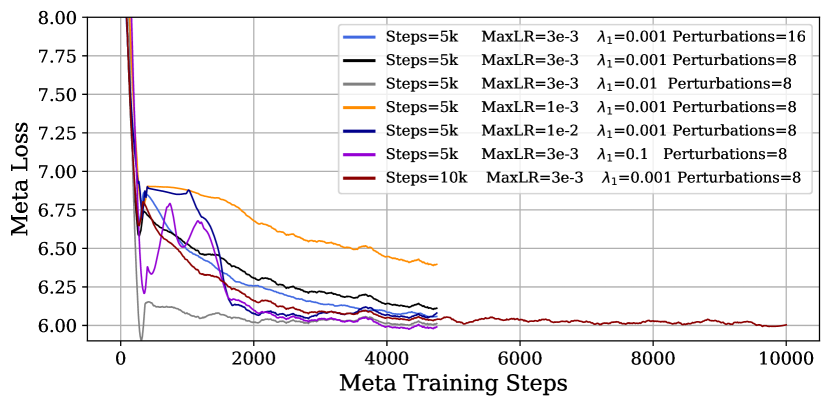
Figure 8: Ablating Meta-training Hyperparameter for $\mu\text{LO}_{S}$. Using AdamW with a linear warmup and cosine annealing schedule, we meta-train $\mu\text{LO}_{S}$ to train 3-layer width 128 MLPs for classifying $32\times 32\times 3$ ImageNet Images. By default, we warmup linearly for 100 steps to a maximum learning rate of $3e-3$ and anneal the learning rate for $4900$ steps to a value of $1e-3$ with $\lambda_{1}=0.001$ (from equation 3) and sampling $8$ perturbations per step in PES[36]. The above ablation varies the maximum learning rate $\in\{1e-2,3e-3,1e-3\}$ (always using $100$ steps of warmup and decaying to $0.3\times$MaxLR), $\lambda_{1}\in\{0.001,0.01,0.1\}$, the number of steps (5k or 10k), and the number of perturbations (8 or 16). We observe that using all default values except for $\lambda_{1}=0.01$ yields one of the best solutions while being fast to train and stable during meta-training.

Appendix E Features of the learned optimizer

Table 3: Per-parameter features used as input to our learned optimizers. All the coefficients, $\beta_{i}$, are learnable parameters adjusted during meta-optimization. We replicate the table of [15] for convenience.

Description	value
parameter value	$w_{t}$
3 momentum values with coefficients $\beta_{1},\beta_{2},\beta_{3}$	$m_{t,i}=\beta_{i}m_{t-1,i}+(1-\beta_{i})g_{t}$
second moment value computed from $g_{t}$ with decay $\beta_{4}$	$v_{t}=\beta_{4}v_{t-1}+(1-\beta_{4})g_{t}^{2}$
3 values consisting of the three momentum values normalized by the square root of the second moment	$\frac{m_{t,i}}{\sqrt{v}}$
the reciprocal square root of the second moment value	$\frac{1}{\sqrt{v}}$
3 $\Delta_{t}$ Adafactor normalized values	$g_{t}\times\textsc{row factor}\times\textsc{column factor}$
3 tiled Adafactor row features with coefficients $\beta_{5},\beta_{6},\beta_{7}$, computed from $g_{t}$	$r_{t,i}=\beta_{i}r_{t-1,i}+(1-\beta_{i})\textsc{row\_mean}(\Delta_{t}^{2})$
3 tiled Adafactor column feature with coefficients $\beta_{5},\beta_{6},\beta_{7}$ computed from $g_{t}$	$c_{t,i}=\beta_{i}c_{t-1,i}+(1-\beta_{i})\textsc{col\_mean}(\Delta_{t}^{2})$
the reciprocal square root of the previous 6 features	$\frac{1}{\sqrt{r_{t,i}\textsc{ or }c_{t,i}}}$
3 $m$ Adafactor normalized values	$m_{t,i}\times\textsc{row factor}\times\textsc{column factor}$

Appendix F Extended Results

F.1 List of Meta-testing Tasks

Table 4 reports the configuration of different testing tasks used to evaluate our optimizers. We note that we do not augment the ImageNet datasets we use in any way except for normalizing the images. We tokenize LM1B using a sentence piece tokenizer[18] with 32k vocabulary size. All evaluation tasks are run on A6000 or A100 GPUs for $5$ random seeds. Each individual run takes less than $2$ hours to complete on a single 80GB A100.

Table 4: Meta-testing settings. We report the optimization tasks we will use to evaluate the LOs of Table 1.

Identifier Dataset Model Depth Width Batch Size Sequence Length ${\mathcal{T}}^{\text{MLP}}_{1}$ $32\times 32$ ImageNet MLP $3$ $128$ $4096$ – ${\mathcal{T}}^{\text{MLP}}_{2}$ $32\times 32$ ImageNet MLP $3$ $512$ $4096$ – ${\mathcal{T}}^{\text{MLP}}_{3}$ $32\times 32$ ImageNet MLP $3$ $2048$ $4096$ – ${\mathcal{T}}^{\text{MLP}}_{4}$ $32\times 32$ ImageNet MLP $3$ $8192$ $4096$ – ${\mathcal{T}}^{\text{MLP}}_{5}$ $64\times 64$ ImageNet MLP $3$ $128$ $4096$ – ${\mathcal{T}}^{\text{MLP}}_{6}$ $64\times 64$ ImageNet MLP $3$ $512$ $4096$ – ${\mathcal{T}}^{\text{MLP}}_{7}$ $64\times 64$ ImageNet MLP $3$ $2048$ $4096$ – ${\mathcal{T}}^{\text{MLP}}_{8}$ $32\times 32$ Cifar-10 MLP $3$ $128$ $4096$ – ${\mathcal{T}}^{\text{MLP}}_{9}$ $32\times 32$ Cifar-10 MLP $3$ $512$ $4096$ – ${\mathcal{T}}^{\text{MLP}}_{10}$ $32\times 32$ Cifar-10 MLP $3$ $2048$ $4096$ – ${\mathcal{T}}^{\text{MLP}}_{11}$ $32\times 32$ Cifar-10 MLP $3$ $8192$ $4096$ – ${\mathcal{T}}^{\text{LM}}_{1}$ LM1B Transformer LM $3$ $192$ $128$ $64$ ${\mathcal{T}}^{\text{LM}}_{2}$ LM1B Transformer LM $3$ $1024$ $128$ $64$ ${\mathcal{T}}^{\text{LM}}_{2}$ LM1B Transformer LM $3$ $2048$ $128$ $64$ ${\mathcal{T}}^{\text{ViT}}_{1}$ $32\times 32$ ImageNet ViT $3$ $192$ $1024$ – ${\mathcal{T}}^{\text{ViT}}_{2}$ $32\times 32$ ImageNet ViT $3$ $1024$ $1024$ – ${\mathcal{T}}^{\text{ViT}}_{2}$ $32\times 32$ ImageNet ViT $3$ $2048$ $1024$ – ${\mathcal{D}}{\mathcal{T}}^{\text{MLP}}_{1}$ $32\times 32$ ImageNet MLP $16$ $512$ $4096$ – ${\mathcal{D}}{\mathcal{T}}^{\text{ViT}}_{1}$ $32\times 32$ ImageNet ViT $16$ $192$ $1024$ – ${\mathcal{D}}{\mathcal{T}}^{\text{LM}}_{1}$ LM1B Transformer LM $16$ $192$ $128$ $64$

F.2 Extended results

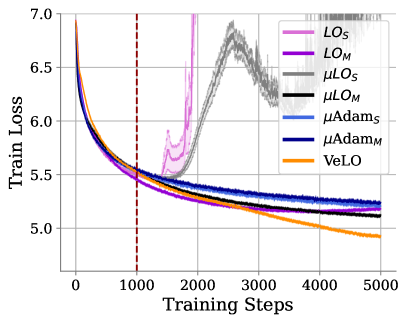
((a))

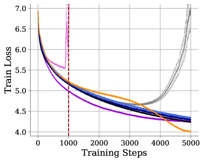
((b))

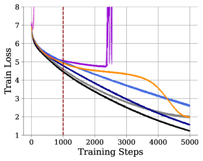
((c))

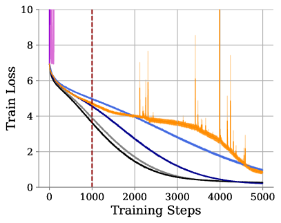
((d))

Figure 9: Evaluating generalization to wider networks. We train MLPs of different sizes to classify $32\times 32\times 3$ ImageNet images. Our optimizers are meta-trained for $1000$ inner steps (dotted red line), therefore, any optimization beyond $1000$ steps is considered out-of-distribution. We observe that $\mu\text{LO}_{M}$ generalize smoothly to all tasks, even surpassing the performance of VeLO (Fig.(c),(d)). We plot average training loss over $5$ seeds with standard error bars.

Appendix G Coordinate evolution of MLP layers in $\mu$P for different optimizers

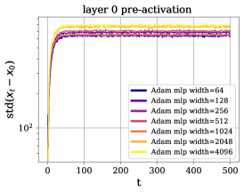
((a))

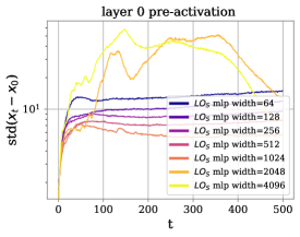
((b))

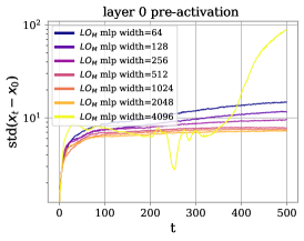
((c))

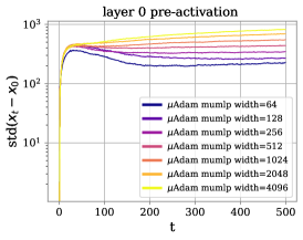
((d))

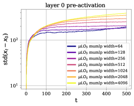
((e))

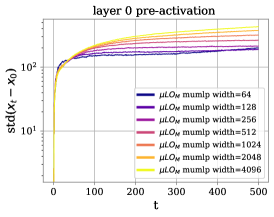
((f))

Figure 11: Layer 0 pre-activations behave harmoniously in $\mu$P for LOs and Adam alike. We report the evolution of coordinate-wise standard deviation between the difference of initial and current second-layer pre-activations. We observe that all models parameterized in $\mu$P enjoy stable coordinates across scales, while the pre-activations of models in SP blow up after a number of training steps.

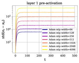
((a))

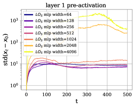
((b))

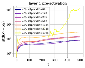
((c))

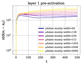
((d))

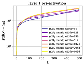
((e))

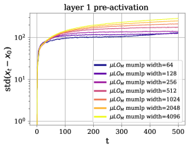
((f))

Figure 12: Layer 1 pre-activations behave harmoniously in $\mu$P for LOs and Adam alike. We report the evolution of coordinate-wise standard deviation between the difference of initial and current second-layer pre-activations. We observe that all models parameterized in $\mu$P enjoy stable coordinates across scales, while the pre-activations of models in SP blow up after a number of training steps.

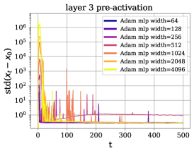
((a))

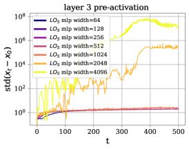
((b))

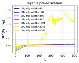
((c))

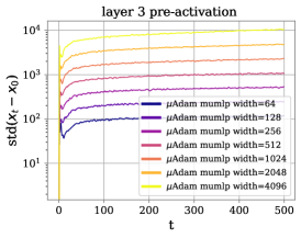
((d))

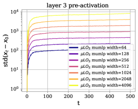
((e))

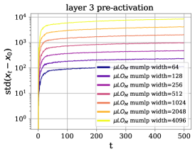
((f))

Figure 13: pre-activations behave harmoniously in $\mu$P for LOs and Adam alike. We report the evolution of coordinate-wise standard deviation between the difference of initial and current second-layer pre-activations. We observe that all models parameterized in $\mu$P enjoy stable coordinates across scales, while the pre-activations of models in SP blow up after a number of training steps.

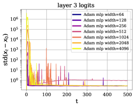
((a))

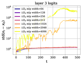
((b))

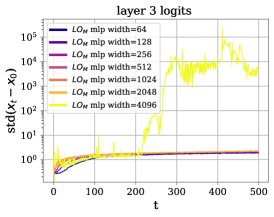
((c))

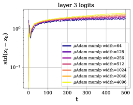
((d))

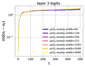
((e))

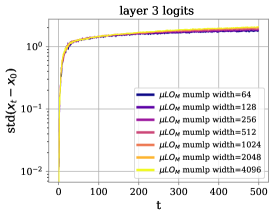
((f))

Figure 14: Logits behave harmoniously in $\mu$P for LOs and Adam alike. We report the evolution of coordinate-wise standard deviation between the difference of initial and current second-layer pre-activations. We observe that all models parameterized in $\mu$P enjoy stable logits across scales, while the pre-activations of models in SP blow up after a number of training steps.

References

- Alayrac et al. [2022] J. Alayrac, J. Donahue, P. Luc, A. Miech, I. Barr, Y. Hasson, K. Lenc, A. Mensch, K. Millican, M. Reynolds, R. Ring, E. Rutherford, S. Cabi, T. Han, Z. Gong, S. Samangooei, M. Monteiro, J. L. Menick, S. Borgeaud, A. Brock, A. Nematzadeh, S. Sharifzadeh, M. Binkowski, R. Barreira, O. Vinyals, A. Zisserman, and K. Simonyan. Flamingo: a visual language model for few-shot learning. In S. Koyejo, S. Mohamed, A. Agarwal, D. Belgrave, K. Cho, and A. Oh, editors, Advances in Neural Information Processing Systems 35: Annual Conference on Neural Information Processing Systems 2022, NeurIPS 2022, New Orleans, LA, USA, November 28 - December 9, 2022, 2022. URL http://papers.nips.cc/paper_files/paper/2022/hash/960a172bc7fbf0177ccccbb411a7d800-Abstract-Conference.html.
- Almeida et al. [2021] D. Almeida, C. Winter, J. Tang, and W. Zaremba. A generalizable approach to learning optimizers. arXiv preprint arXiv:2106.00958, 2021.
- Amos [2022] B. Amos. Tutorial on amortized optimization for learning to optimize over continuous domains. arXiv e-prints, pages arXiv–2202, 2022.
- Andrychowicz et al. [2016] M. Andrychowicz, M. Denil, S. Gomez, M. W. Hoffman, D. Pfau, T. Schaul, B. Shillingford, and N. De Freitas. Learning to learn by gradient descent by gradient descent. Advances in neural information processing systems, 29, 2016.
- Brooks et al. [2024] T. Brooks, B. Peebles, C. Homes, W. DePue, Y. Guo, L. Jing, D. Schnurr, J. Taylor, T. Luhman, E. Luhman, C. W. Y. Ng, R. Wang, and A. Ramesh. Video generation models as world simulators. 2024. URL https://openai.com/research/video-generation-models-as-world-simulators.
- Brown et al. [2020] T. B. Brown, B. Mann, N. Ryder, M. Subbiah, J. Kaplan, P. Dhariwal, A. Neelakantan, P. Shyam, G. Sastry, A. Askell, et al. Language models are few-shot learners. In Proceedings of the 34th International Conference on Neural Information Processing Systems, pages 1877–1901, 2020. URL https://arxiv.org/abs/2005.14165.
- Buckman et al. [2018] J. Buckman, D. Hafner, G. Tucker, E. Brevdo, and H. Lee. Sample-efficient reinforcement learning with stochastic ensemble value expansion. In S. Bengio, H. M. Wallach, H. Larochelle, K. Grauman, N. Cesa-Bianchi, and R. Garnett, editors, Advances in Neural Information Processing Systems 31: Annual Conference on Neural Information Processing Systems 2018, NeurIPS 2018, December 3-8, 2018, Montréal, Canada, pages 8234–8244, 2018. URL https://proceedings.neurips.cc/paper/2018/hash/f02208a057804ee16ac72ff4d3cec53b-Abstract.html.
- Chelba et al. [2013] C. Chelba, T. Mikolov, M. Schuster, Q. Ge, T. Brants, and P. Koehn. One billion word benchmark for measuring progress in statistical language modeling. CoRR, abs/1312.3005, 2013. URL http://arxiv.org/abs/1312.3005.
- Chen et al. [2020] T. Chen, W. Zhang, Z. Jingyang, S. Chang, S. Liu, L. Amini, and Z. Wang. Training stronger baselines for learning to optimize. Advances in Neural Information Processing Systems, 33:7332–7343, 2020.
- Chen et al. [2022] T. Chen, X. Chen, W. Chen, Z. Wang, H. Heaton, J. Liu, and W. Yin. Learning to optimize: A primer and a benchmark. The Journal of Machine Learning Research, 23(1):8562–8620, 2022.
- Dalal and Triggs [2005] N. Dalal and B. Triggs. Histograms of oriented gradients for human detection. In 2005 IEEE Computer Society Conference on Computer Vision and Pattern Recognition (CVPR’05), volume 1, pages 886–893 vol. 1, 2005. doi: 10.1109/CVPR.2005.177.
- Dosovitskiy et al. [2020] A. Dosovitskiy, L. Beyer, A. Kolesnikov, D. Weissenborn, X. Zhai, T. Unterthiner, M. Dehghani, M. Minderer, G. Heigold, S. Gelly, et al. An image is worth 16x16 words: Transformers for image recognition at scale. arXiv preprint arXiv:2010.11929, 2020.
- Goodfellow et al. [2016] I. Goodfellow, Y. Bengio, and A. Courville. Deep Learning. MIT Press, 2016. http://www.deeplearningbook.org.
- Harrison et al. [2022] J. Harrison, L. Metz, and J. Sohl-Dickstein. A closer look at learned optimization: Stability, robustness, and inductive biases. Advances in Neural Information Processing Systems, 35:3758–3773, 2022.
- Joseph et al. [2023] C. Joseph, B. Thérien, A. Moudgil, B. Knyazev, and E. Belilovsky. Can we learn communication-efficient optimizers? CoRR, abs/2312.02204, 2023. URL https://doi.org/10.48550/arXiv.2312.02204.
- Kingma and Ba [2017] D. P. Kingma and J. Ba. Adam: A method for stochastic optimization, 2017.
- Kirillov et al. [2023] A. Kirillov, E. Mintun, N. Ravi, H. Mao, C. Rolland, L. Gustafson, T. Xiao, S. Whitehead, A. C. Berg, W.-Y. Lo, P. Dollár, and R. Girshick. Segment anything. arXiv:2304.02643, 2023.
- Kudo and Richardson [2018] T. Kudo and J. Richardson. Sentencepiece: A simple and language independent subword tokenizer and detokenizer for neural text processing. In E. Blanco and W. Lu, editors, Proceedings of the 2018 Conference on Empirical Methods in Natural Language Processing, EMNLP 2018: System Demonstrations, Brussels, Belgium, October 31 - November 4, 2018, pages 66–71. Association for Computational Linguistics, 2018. URL https://doi.org/10.18653/v1/d18-2012.
- Li et al. [2023] H. Li, A. Rakhlin, and A. Jadbabaie. Convergence of adam under relaxed assumptions. In A. Oh, T. Naumann, A. Globerson, K. Saenko, M. Hardt, and S. Levine, editors, Advances in Neural Information Processing Systems 36: Annual Conference on Neural Information Processing Systems 2023, NeurIPS 2023, New Orleans, LA, USA, December 10 - 16, 2023, 2023. URL http://papers.nips.cc/paper_files/paper/2023/hash/a3cc50126338b175e56bb3cad134db0b-Abstract-Conference.html.
- Loshchilov and Hutter [2019] I. Loshchilov and F. Hutter. Decoupled weight decay regularization. In 7th International Conference on Learning Representations, ICLR 2019, New Orleans, LA, USA, May 6-9, 2019. OpenReview.net, 2019. URL https://openreview.net/forum?id=Bkg6RiCqY7.
- Lowe [2004] D. G. Lowe. Distinctive image features from scale-invariant keypoints. Int. J. Comput. Vis., 60(2):91–110, 2004. URL https://doi.org/10.1023/B:VISI.0000029664.99615.94.
- Metz et al. [2019] L. Metz, N. Maheswaranathan, J. Nixon, D. Freeman, and J. Sohl-Dickstein. Understanding and correcting pathologies in the training of learned optimizers. In International Conference on Machine Learning, pages 4556–4565. PMLR, 2019.
- Metz et al. [2022a] L. Metz, C. D. Freeman, J. Harrison, N. Maheswaranathan, and J. Sohl-Dickstein. Practical tradeoffs between memory, compute, and performance in learned optimizers, 2022a.
- Metz et al. [2022b] L. Metz, J. Harrison, C. D. Freeman, A. Merchant, L. Beyer, J. Bradbury, N. Agrawal, B. Poole, I. Mordatch, A. Roberts, et al. Velo: Training versatile learned optimizers by scaling up. arXiv preprint arXiv:2211.09760, 2022b.
- Nesterov and Spokoiny [2017] Y. E. Nesterov and V. G. Spokoiny. Random gradient-free minimization of convex functions. Found. Comput. Math., 17(2):527–566, 2017. URL https://doi.org/10.1007/s10208-015-9296-2.
- Oquab et al. [2023] M. Oquab, T. Darcet, T. Moutakanni, H. V. Vo, M. Szafraniec, V. Khalidov, P. Fernandez, D. Haziza, F. Massa, A. El-Nouby, R. Howes, P.-Y. Huang, H. Xu, V. Sharma, S.-W. Li, W. Galuba, M. Rabbat, M. Assran, N. Ballas, G. Synnaeve, I. Misra, H. Jegou, J. Mairal, P. Labatut, A. Joulin, and P. Bojanowski. Dinov2: Learning robust visual features without supervision, 2023.
- Parmas et al. [2018] P. Parmas, C. E. Rasmussen, J. Peters, and K. Doya. PIPPS: flexible model-based policy search robust to the curse of chaos. In J. G. Dy and A. Krause, editors, Proceedings of the 35th International Conference on Machine Learning, ICML 2018, Stockholmsmässan, Stockholm, Sweden, July 10-15, 2018, volume 80 of Proceedings of Machine Learning Research, pages 4062–4071. PMLR, 2018. URL http://proceedings.mlr.press/v80/parmas18a.html.
- Premont-Schwarz et al. [2022] I. Premont-Schwarz, J. Vitkuu, and J. Feyereisl. A simple guard for learned optimizers. arXiv preprint arXiv:2201.12426, 2022.
- Radford et al. [2021] A. Radford, J. W. Kim, C. Hallacy, A. Ramesh, G. Goh, S. Agarwal, G. Sastry, A. Askell, P. Mishkin, J. Clark, G. Krueger, and I. Sutskever. Learning transferable visual models from natural language supervision. In M. Meila and T. Zhang, editors, Proceedings of the 38th International Conference on Machine Learning, ICML 2021, 18-24 July 2021, Virtual Event, volume 139 of Proceedings of Machine Learning Research, pages 8748–8763. PMLR, 2021. URL http://proceedings.mlr.press/v139/radford21a.html.
- Robbins [1951] H. E. Robbins. A stochastic approximation method. Annals of Mathematical Statistics, 22:400–407, 1951. URL https://api.semanticscholar.org/CorpusID:16945044.
- Rombach et al. [2022] R. Rombach, A. Blattmann, D. Lorenz, P. Esser, and B. Ommer. High-resolution image synthesis with latent diffusion models. In IEEE/CVF Conference on Computer Vision and Pattern Recognition, CVPR 2022, New Orleans, LA, USA, June 18-24, 2022, pages 10674–10685. IEEE, 2022. URL https://doi.org/10.1109/CVPR52688.2022.01042.
- Schmidhuber [1992] J. Schmidhuber. Learning to control fast-weight memories: An alternative to dynamic recurrent networks. Neural Computation, 4(1):131–139, 1992.
- Spall [2000] J. C. Spall. Adaptive stochastic approximation by the simultaneous perturbation method. IEEE Trans. Autom. Control., 45(10):1839–1853, 2000. URL https://doi.org/10.1109/TAC.2000.880982.
- Thrun and Pratt [2012] S. Thrun and L. Pratt. Learning to learn. Springer Science & Business Media, 2012.
- Vicol [2023] P. Vicol. Low-variance gradient estimation in unrolled computation graphs with es-single. In International Conference on Machine Learning, pages 35084–35119. PMLR, 2023.
- Vicol et al. [2021] P. Vicol, L. Metz, and J. Sohl-Dickstein. Unbiased gradient estimation in unrolled computation graphs with persistent evolution strategies. In M. Meila and T. Zhang, editors, Proceedings of the 38th International Conference on Machine Learning, ICML 2021, 18-24 July 2021, Virtual Event, volume 139 of Proceedings of Machine Learning Research, pages 10553–10563. PMLR, 2021. URL http://proceedings.mlr.press/v139/vicol21a.html.
- Wichrowska et al. [2017] O. Wichrowska, N. Maheswaranathan, M. W. Hoffman, S. G. Colmenarejo, M. Denil, N. Freitas, and J. Sohl-Dickstein. Learned optimizers that scale and generalize. In International conference on machine learning, pages 3751–3760. PMLR, 2017.
- Yang [2019] G. Yang. Tensor programs I: wide feedforward or recurrent neural networks of any architecture are gaussian processes. CoRR, abs/1910.12478, 2019. URL http://arxiv.org/abs/1910.12478.
- Yang [2020a] G. Yang. Tensor programs II: neural tangent kernel for any architecture. CoRR, abs/2006.14548, 2020a. URL https://arxiv.org/abs/2006.14548.
- Yang [2020b] G. Yang. Tensor programs III: neural matrix laws. CoRR, abs/2009.10685, 2020b. URL https://arxiv.org/abs/2009.10685.
- Yang and Hu [2021] G. Yang and E. J. Hu. Tensor programs IV: feature learning in infinite-width neural networks. In M. Meila and T. Zhang, editors, Proceedings of the 38th International Conference on Machine Learning, ICML 2021, 18-24 July 2021, Virtual Event, volume 139 of Proceedings of Machine Learning Research, pages 11727–11737. PMLR, 2021. URL http://proceedings.mlr.press/v139/yang21c.html.
- Yang and Littwin [2023] G. Yang and E. Littwin. Tensor programs ivb: Adaptive optimization in the infinite-width limit. CoRR, abs/2308.01814, 2023. URL https://doi.org/10.48550/arXiv.2308.01814.
- Yang et al. [2022] G. Yang, E. J. Hu, I. Babuschkin, S. Sidor, D. Farhi, J. Pachocki, X. Liu, W. Chen, and J. Gao. Tensor programs v: Tuning large neural networks via zero-shot hyperparameter transfer. In NeurIPS 2021, March 2022. URL https://www.microsoft.com/en-us/research/publication/tuning-large-neural-networks-via-zero-shot-hyperparameter-transfer/.
- Yang et al. [2023] J. Yang, T. Chen, M. Zhu, F. He, D. Tao, Y. Liang, and Z. Wang. Learning to generalize provably in learning to optimize. In International Conference on Artificial Intelligence and Statistics, pages 9807–9825. PMLR, 2023.