Submodular Maximization in Exactly $n$ Queries

Abstract

In this work, we study the classical problem of maximizing a submodular function subject to a matroid constraint. We develop deterministic algorithms that are very parsimonious with respect to querying the submodular function, for both the case when the submodular function is monotone and the general submodular case. In particular, we present a $1/4$ approximation algorithm for the monotone case that uses exactly one query per element, which gives the same total number of queries $n$ as the number of queries required to compute the maximum singleton. For the general case, we present a constant factor approximation algorithm that requires $2$ queries per element, which is the first algorithm for this problem with linear query complexity in the size of the ground set.

1 Introduction

Submodular optimization.

Many objectives that we aim to optimize in machine learning, such as coverage, diversity, and entropy, satisfy the diminishing returns property required for a function to be submodular. Submodular maximization algorithms are thus employed in applications such as document summarization [27], influence maximization in networks [19], recommender systems [4], and feature selection [12]. A fundamental problem in this field is to maximize a monotone submodular function under a matroid constraint, which we refer to as MSM. For this problem, the celebrated greedy algorithm of Fisher et al. [16] achieves a $1/2$ approximation. This $1/2$ approximation was improved by Calinescu et al. [9] to $1-1/e$ with a continuous greedy algorithm, which is the best approximation achievable with polynomially many queries [30]. The broader problem of maximizing a, not necessarily monotone, submodular function under a cardinality constraint, which we refer to as GSM, is also known to admit constant factor approximation algorithms [24].

Fast algorithms for MSM.

Due to the many applications of submodular maximization over massive datasets, a major focus has been to develop fast algorithms for submodular maximization (see, e.g., [2, 29, 14, 6, 22, 26]). Since the time required to perform function evaluations usually dominates other parts of the computation, the speed of an algorithm is often measured by its query complexity, i.e., its number of function evaluations. In particular, the query complexity of the greedy algorithm is $kn$, where $k$ is the rank of the matroid and $n$ is size of the ground set. Badanidiyuru and Vondrák [2] improved this query complexity with an algorithm with $\mathcal{O}\left((n/\varepsilon)\log(k/\varepsilon)\right)$ query complexity that achieves a $1/2-\varepsilon$ approximation for MSM. Subsequently, Chakrabarti and Kale [10] achieved a linear query complexity with a $1/4$-approximation algorithm that makes at most $2n$ queries. On the hardness side, Kuhnle [22] showed that $n$ queries are required to obtain an approximation of $1/2+\varepsilon$, even for the special case of finding the maximum singleton.

Fast algorithms for GSM.

If the objective function is not monotone, there are no known algorithms with linear query complexity. Lee et al. [24] obtained the first constant factor approximation algorithm for GSM, with an algorithm that has query complexity $\tilde{O}(n^{4})$. An algorithm of Kuhnle [21] achieves a ratio $1/4-\varepsilon$ in $\mathcal{O}\left(\frac{n}{\varepsilon}\log\frac{k}{\varepsilon}\right)$ queries for the special case of a size constraint, and this algorithm was extended to handle a matroid constraint by Han et al. [18], keeping the same ratio and query complexity. Since the rank $k$ may be as large as $n$, the query complexity of these algorithms is superlinear in the size of the ground set.

The main question we ask in this paper is whether the best-known query complexity for these two problems can be improved while achieving a constant factor approximation guarantee.

What is the query complexity of achieving a constant factor approximation for MSM and GSM?

Our results.

Our first main result shows that $n$ queries are sufficient to achieve a constant factor approximation with a deterministic algorithm for MSM.

Theorem.

There is a deterministic $1/4$-approximation algorithm for MSM with query complexity $n$.

This result improves the query complexity of Chakrabarti and Kale [10] from $2n$ to $n$, while maintaining the same approximation. We emphasize that our algorithm, called QuickSwap, does a pass over the elements and performs a single query per element. The main idea needed to perform only a single query per element $e$ requires maintaining an infeasible solution and evaluating the marginal contribution of $e$ to this infeasible solution, whereas the vast majority of algorithms for submodular maximization only maintain a feasible solution. In fact, there have been lower bounds for submodular maximization that make the assumption that the algorithm only queries feasible sets [31, 23], and this has been considered a natural assumption. Whether our result can be achieved by only querying feasible sets is an interesting question for future work. This $n$ query complexity matches the number of queries required to find the element $e$ with maximum singleton value $f(\{e\})$ [22].

Our second main result is the first constant factor approximation algorithm with linear query complexity for GSM.

Theorem.

There is a deterministic $1/(6+4\sqrt{2})\approx 1/11.66$-approximation algorithm for GSM with query complexity $2n$.

The previous best query complexity achieved by a constant factor approximation algorithm for GSM is $\mathcal{O}\left(\frac{n}{\varepsilon}\log\frac{k}{\varepsilon}\right)$. In addition to achieving the first linear query complexity algorithm for this problem, we emphasize that another benefit of our algorithm is that the query complexity does not depend on large constants, which is important for the practicality of the algorithm. We emphasize that the algorithm and its analysis for GSM build on the QuickSwap algorithm for MSM.

Finally, we empirically demonstrate the practicality of QuickSwap. On real and synthetic datasets, it always achieves an improved number of queries and a similar objective value as the algorithm of Chakrabarti and Kale [10] with $2n$ queries. Compared to the lazy greedy algorithm and the algorithm of Badanidiyuru and Vondrák [2], it achieves a significant improvement in the number of queries at a small cost in the objective value.

1.1 Related work

Linear-Time Algorithms for Size and Knapsack Constraints.

For the special case of monotone submodular maximization under a size constraint, two works [22, 26] independently achieved an $\mathcal{O}\left((n/\varepsilon)\log(1/\varepsilon)\right)$ query complexity and a nearly optimal $1-1/e-\varepsilon$ approximation ratio. These are the first deterministic algorithms to achieve nearly the $1-1/e$ ratio for size constraints with linear query complexity. Li et al. [26] also provide an $\mathcal{O}_{\varepsilon}\left(n\log n\right)$ algorithm for the intersection of matroid and $\ell$ knapsack constraints; however, for the case of a single matroid and zero knapsacks, this algorithm reduces to the $1/2-\varepsilon$-approximation algorithm in [2] previously discussed.

Relationship to Kuhnle [22].

For MSM under size constraint, Kuhnle [22] provides the algorithm QuickStream, a $(1/4)$-approximation algorithm in exactly $n$ queries. Our algorithm shares some common features with this algorithm: both algorithms query an infeasible set to determine whether to add an element. However, QuickStream uses multiple ideas that are specific to size constraint which do not generalize to matroid constraints. Most importantly, it relies upon the fact that the last $k$ elements added to the infeasible set form a feasible set. This fact, together with the condition to add an element, is crucial for proving the $1/4$ ratio of QuickStream. Unfortunately, for the matroid constraint, one cannot find a feasible set in this way. A different strategy for maintaining a feasible subset of the infeasible set is required, together with a different strategy for adding an element.

We also note that for size constraint, Kuhnle [22] gave a technique to transform any $\alpha$-approximation deterministic algorithm with query complexity $q$ into an $\alpha/c$-approximation deterministic algorithm with query complexity $q/c$, for any integer $c$. However, this technique does not work for matroid constraints. Another technique to reduce the query complexity at the cost of the approximation ratio is to run an algorithm on a randomly sampled subset of the ground set. However, the approximation guarantees with this approach only hold in expectation, instead of deterministically, and the sampling also causes a loss in approximation. In particular, for GSM, this technique cannot be used with an existing algorithm to achieve a constant approximation and a linear query complexity.

Relationship to Chakrabarti and Kale [10].

As mentioned above, Chakrabarti and Kale [10] developed a streaming algorithm for the monotone problem that achieves the same ratio as our algorithm in at most $2n$ queries. Their algorithm takes one pass through the ground set and maintains a feasible set through the following swapping logic. Each element is assigned a weight (which requires at most two queries to the oracle), and the feasible solution is updated via appealing to an algorithm of Ashwinkumar [1] for maximum (modular) weight independent set. By contrast, our monotone algorithm employs a single query to an infeasible set to determine whether two elements should be swapped. In our empirical evaluation (Section 4), we show that the two algorithms obtain a similar objective value, but our algorithm uses fewer queries.

Relationship to Feldman et al. [15].

Feldman et al. [15] developed several streaming algorithms for the general problem GSM. These algorithms also take one pass through the ground set and decide whether it makes sense to swap out an existing element for a new candidate. These algorithms employ many queries to the submodular function to determine if a swap should be made: $O(k)$ queries are required per element in the worst case, where $k$ is the rank of the matroid. By contrast, our general algorithm makes two queries to two infeasible sets to determine if an element should be swapped. However, we should note that the graph constructions required to prove our approximation ratios are inspired by the graph constructions used in the analysis of these algorithms.

Faster algorithms that achieve optimal ratio for MSM.

Several works have improved the number of queries needed to obtain the optimal $1-1/e$ ratio for MSM [2, 8, 20]. Very recently, a ratio of $1-1/e-\varepsilon$ was achieved with $\mathcal{O}(\sqrt{k}\,n\,\text{poly}(1/\varepsilon,\log n))$ queries [20].

1.2 Preliminaries

A function $f:2^{\mathcal{N}}\rightarrow\mathbb{R}_{\geq 0}$ is submodular if it satisfies the following diminishing returns property: for all sets $S\subseteq T\subseteq\mathcal{N}$ and any element $a\in\mathcal{N}\setminus T$, we have $f(a|S)\geq f(a|T)$, where $f(a|S)=f(S+a)-f(S)$ is the marginal contribution of $a$ to $S$. Equivalently, $f$ is submodular if $f(S)+f(T)\geq f(S\cup T)+f(S\cap T)$ for all sets $S,T\subseteq\mathcal{N}$. It is monotone if $f(S)\leq f(T)$ for all sets $S\subseteq T\subseteq\mathcal{N}$.

Let $\mathcal{I}\subseteq 2^{\mathcal{N}}$ be a collection of subsets of $\mathcal{N}$. Then $\mathcal{M}=(\mathcal{N},\mathcal{I})$ is a matroid if the following three properties are satisfied: (1) $\emptyset\in\mathcal{I}$,   (2) for all sets $S\subseteq T\subseteq\mathcal{N}$, if $T\in\mathcal{I}$ then $S\in\mathcal{I}$ (downward-closed property), and   (3) for all sets $S,T\subseteq\mathcal{N}$ such that $|S|<|T|$, there exists $e\in T\setminus S$ such that $S+e\in\mathcal{I}$ (augmentation property).

In the submodular maximization under a matroid constraint problem (GSM), we are given a submodular function $f:2^{\mathcal{N}}\rightarrow\mathbb{R}_{\geq 0}$ and a matroid $\mathcal{M}=(\mathcal{N},\mathcal{I})$, and the goal is to approximately solve $\max_{S\in\mathcal{I}}f(S)$. In the monotone submodular maximization under a matroid constraint problem (MSM), the function $f$ is assumed to also be monotone. A set $S\in\mathcal{I}$ is interchangeably called independent or feasible. We assume without loss of generality that $\{e\}\in\mathcal{I}$ for all $e\in\mathcal{N}$.

The algorithm is given access to a value oracle for $f$, i.e., it can query the value $f(S)$ of any set $S\subseteq\mathcal{N}$, as well as an independence oracle for $\mathcal{M}$, i.e., it can test whether $S\in\mathcal{I}$ or $S\not\in\mathcal{I}$ for any set $S\subseteq\mathcal{N}$. In submodular maximization, the main bottleneck for the running time is typically the function evaluations $f(S)$, so we are interested in designing algorithms for MSM and GSM with low query complexity, which is the worst-case number of queries made by the algorithm to the value oracle for $f$.

2 An approximation algorithm for MSM in exactly $n$ queries

In this section, we present our $(1/4)$-approximation algorithm for MSM that uses exactly $n$ queries. Monotonicity is used in only one place in the analysis, and we also invoke the lemmata proved here in Section 3, where we develop a constant-factor algorithm for GSM with $2n$ query complexity.

Description of the algorithm.

In overview, the algorithm makes a single pass through the ground set, and each element is swapped into the solution $A^{\prime}$ if it is good enough relative to the element it displaces. The novelty lies in the fact that each element is considered to be swapped into $A^{\prime}$ only once; and the definition of good enough relies upon a single query of the marginal gain of the element to an infeasible set $A\supseteq A^{\prime}$ when it arrives.

Specifically, the algorithm maintains two sets, $A^{\prime}\subseteq A$; $A^{\prime}$ is always a feasible solution, and $A$ contains all elements that were once a member of $A^{\prime}$. On Line 1, the weight $\delta_{e}$ of element $e$ is defined as its marginal gain into $A$: $\delta_{e}=f(e|A)$. Since $f(A)$ is already known, computing the gain requires a single query: $f(A+e)$. The weight $\delta_{e}$ is fixed upon arrival of $e$ and never recomputed, and is used for all processing related to $e$. Next, the best candidate to swap $e$ into $A^{\prime}$ is found, according to the weights $\delta$. This element, denoted $a^{*}$, is chosen to be a smallest weight element such that $A^{\prime}\setminus a^{*}+e$ is feasible; that is, $a^{*}=\operatorname*{argmin}_{a\in A^{\prime}|A^{\prime}\setminus a+e\in\mathcal{I}}\delta_{a}$. If $\delta_{e}$ is large enough relative to $\delta_{a^{*}}$, then the swap occurs: $A^{\prime}$ is updated to $A^{\prime}\setminus a^{*}+e$, and $A$ is updated to $A+e$ (and the value of $f(A)$ is updated to $f(A)+\delta_{e}$).

1 Input: Oracle to $f$, ground set $\mathcal{N}$, independence oracle for $\mathcal{M}=(\mathcal{N},\mathcal{I})$, parameter $\beta$

2 $A,A^{\prime}\leftarrow\emptyset$

3 for $e\in\mathcal{N}$ do

4      $\delta_{e}\leftarrow f(e|A)$

5      if $A^{\prime}+e\in\mathcal{I}$ and $\delta_{e}\geq 0$ then

6           $A\leftarrow A+e$

7           $A^{\prime}\leftarrow A^{\prime}+e$

8          

9           else

10                $a^{*}\leftarrow\operatorname*{argmin}_{a\in A^{\prime}|A^{\prime}-a+e\in\mathcal{I}}\delta_{a}$

11                if $\delta_{e}\geq(1+\beta)\delta_{a^{*}}$ then

12                     $A\leftarrow A+e$

13                     $A^{\prime}\leftarrow A^{\prime}-a^{*}+e$

14                    

15                    

Return $A^{\prime}$

Algorithm 1 QuickSwap: A $\frac{1}{4}$-approximation algorithm for monotone submodular maximization under a matroid constraint

2.1 Overview of analysis

The analysis proceeds by first relating $f(A)$ and $f(A^{\prime})$ (Lemma 2.1), then $\textsc{Opt}=f(O)$, $f(A)$, and $f(A^{\prime})$ (Lemma 2.2). We state these two lemmata, then prove the approximation ratio. Subsequently, we prove the lemmata in Sections 2.2 and 2.3, respectively. Both lemmata hold for general, submodular functions, which will be needed in Section 3. Finally, we show that the $1/4$ ratio is tight, with a set of tight examples in Section 2.4.

Lemma 2.1 relates $f(A^{\prime})$ and $f(A)$; intuitively, because $A^{\prime}\subseteq A$ and $\delta_{e}=f(e|A)$, then by submodularity and the condition to swap $a^{*}$ for $e$, the $f$-value of $A^{\prime}$ increases by a constant fraction of the increase in the $f$-value of $A$, despite the loss from $a^{*}$.

Lemma 2.1.

Let $(f,\mathcal{M})$ be an instance of GSM, and let $A^{\prime},A$ be produced by Alg. 1 on this instance. Then $f(A^{\prime})\geq\frac{\beta f(A)}{1+\beta}$.

Next, Lemma 2.2 establishes a relationship between $f(O\cup A)$, $f(A)$, and $f(A^{\prime})$. Intuitively, the rejected elements $O\setminus A$ can each be mapped to an element of $A^{\prime}$ responsible for the rejection. The key fact, which much of the proof is devoted to showing, is that this mapping is injective. That is, each element $o$ of $O\setminus A$ can be mapped to a unique element of $A^{\prime}$, which may be thought of as gatekeeper for the element $o$. To prove the mapping is an injection, a graph construction is employed.

Lemma 2.2.

Let $(f,\mathcal{M})$ be an instance of GSM with optimal solution $O$, and let $A^{\prime},A$ be produced by Alg. 1 on this instance. Then $f(O\cup A)\leq f(A)+(1+\beta)f(A^{\prime})$.

The approximation follows directly from these two lemmata, as summarized in the following theorem.

Theorem 2.1.

Algorithm 1 is a $(1/4)$-approximation algorithm for MSM with query complexity $n$.

Proof.

Let $e_{i}$, $A_{i}$, and $A^{\prime}_{i}$ denote the element $e$, the set $A$, and the set $A^{\prime}$ at iteration $i$ of the algorithm. For the query complexity, note that at iteration $i$, the algorithm evaluates $f(e_{i}|A_{i-1})=f(A_{i-1}+e_{i})-f(A_{i-1})$. Let $e_{j}$ be the last element added to $A$ such that $j<i$. If there is no such $j$, then $A_{i-1}=\emptyset$ and $f(A_{i-1})=0$. Otherwise, we have $A_{i-1}=A_{j}=A_{j-1}+e_{j}$ and query $f(A_{i-1})=f(A_{j-1}+e_{j})$ was already performed at iteration $j$. Thus, only one query to $f$ is needed at each iteration and the query complexity is $n$. For the approximation, observe that

$$f(O)\leq_{(1)}f(O\cup A)<_{(2)}f(A)+(1+\beta)f(A^{\prime})\leq_{(3)}\frac{(\beta+1)^{2}}{\beta}f(A^{\prime}),$$

where $(1)$ is by monotonicity, $(2)$ is by Lemma 2.2, and $(3)$ is by Lemma 2.1. The $1/4$ ratio follows from optimizing over $\beta\in[0,\infty)$ (the ratio is optimized at $\beta=1$). ∎

2.2 Proof of Lemma 2.1

We first give a helper lemma, which relates the change in the sum of the weights of elements in $A^{\prime}$ to the same sum for $A$, for a single iteration.

Lemma 2.3.

Let $f$ be a submodular function (not necessarily monotone). Then, for any $i\in[n],$ we have that $\sum_{e_{j}\in A^{\prime}_{i}}\delta_{e_{j}}-\sum_{e_{j}\in A^{\prime}_{i-1}}\delta_{e_{j}}\geq\frac{\beta}{1+\beta}\left(\sum_{e_{j}\in A_{i}}\delta_{e_{j}}-\sum_{e_{j}\in A_{i-1}}\delta_{e_{j}}\right).$

Proof.

There are three cases. Case 1: if $A^{\prime}_{i-1}+e_{i}\in M$ and $\delta_{e_{i}}\geq 0$. Then, we have $A_{i}=A_{i-1}+e_{i}$ and $A^{\prime}_{i}=A^{\prime}_{i-1}+e_{i}.$ We get that

$$\sum_{e_{j}\in A^{\prime}_{i}}\delta_{e_{j}}-\sum_{e_{j}\in A^{\prime}_{i-1}}\delta_{e_{j}}=\delta_{e_{i}}\geq_{(1)}\frac{\beta\delta_{e_{i}}}{1+\beta}=\frac{\beta}{1+\beta}\left(\sum_{e_{j}\in A_{i}}\delta_{e_{j}}-\sum_{e_{j}\in A_{i-1}}\delta_{e_{j}}\right),$$

where $(1)$ is since $\delta_{e_{i}}\geq 0$. Case 2: If $A^{\prime}_{i-1}+e_{i}\in M$ and $\delta_{e_{i}}\geq 0$ do not hold and $\delta_{e_{i}}\geq(1+\beta)\delta_{a^{*}}$ does hold. This is the main case for this proof. In this case, we have $A_{i}=A_{i-1}+e_{i}$ and $A^{\prime}_{i}=A^{\prime}_{i-1}-a^{*}+e_{i}.$ We get that

$$\sum_{e_{j}\in A^{\prime}_{i}}\delta_{e_{j}}-\sum_{e_{j}\in A^{\prime}_{i-1}}\delta_{e_{j}}=_{(1)}\delta_{e_{i}}-\delta_{a^{*}}\geq_{(2)}\frac{\beta}{1+\beta}\delta_{e_{i}}=_{(3)}\frac{\beta}{1+\beta}\left(\sum_{e_{j}\in A_{i}}\delta_{e_{j}}-\sum_{e_{j}\in A_{i-1}}\delta_{e_{j}}\right).$$

where $(1)$ is since $A^{\prime}_{i}=A^{\prime}_{i-1}-a^{*}+e_{i}$, $(2)$ since $\delta_{e_{i}}\geq(1+\beta)\delta_{a^{*}}$, and $(3)$ since $A_{i}=A_{i-1}+e_{i}$. Case 3: if neither conditions hold for the two previous cases, we have that $A_{i}=A_{i-1}$ and $A^{\prime}_{i}=A^{\prime}_{i-1}$. This implies that $\sum_{e_{j}\in A^{\prime}_{i}}\delta_{e_{j}}-\sum_{e_{j}\in A^{\prime}_{i-1}}\delta_{e_{j}}=0$ and $\sum_{e_{j}\in A_{i}}\delta_{e_{j}}-\sum_{e_{j}\in A_{i-1}}\delta_{e_{j}}=0$, and we trivially obtain the desired claim. ∎

We are now ready to prove Lemma 2.1.

Proof of Lemma 2.1.

We first claim that $A^{\prime}_{n}\cap\{e_{1},\ldots,e_{j-1}\}\subseteq A_{j-1}$. Consider $e_{i}\in A^{\prime}_{n}\cap\{e_{1},\ldots,e_{j-1}\}$, so $i\leq j-1$. Since $e_{i}\in A^{\prime}_{n},$ we have $e_{i}\in A^{\prime}_{i}$ by definition of the algorithm. Since $i\leq j-1$, we have $A^{\prime}_{i}\subseteq A_{i}\subseteq A_{j-1}$. Since $e_{i}\in A^{\prime}_{i}$ and $A^{\prime}_{i}\subseteq A_{j-1}$, we get $e_{i}\in A_{j-1}$, which proves the desired claim. We get that

$$f(A^{\prime}_{n}) =\sum_{e_{j}\in A^{\prime}_{n}}f(e_{j}|A^{\prime}_{n}\cap\{e_{1},\ldots,e_{j-1}\})$$

$$\geq\sum_{e_{j}\in A^{\prime}_{n}}\delta_{e_{j}} A^{\prime}_{n}\cap\{e_{1},\ldots,e_{j-1}\}\subseteq A_{j-1}$$

$$=\sum_{i=1}^{n}\left(\sum_{e_{j}\in A^{\prime}_{i}}\delta_{e_{j}}-\sum_{e_{j}\in A^{\prime}_{i-1}}\delta_{e_{j}}\right)$$ telescoping sum

$$\geq\sum_{i=1}^{n}\frac{\beta}{1+\beta}\left(\sum_{e_{j}\in A_{i}}\delta_{e_{j}}-\sum_{e_{j}\in A_{i-1}}\delta_{e_{j}}\right)$$ Lemma 2.3

$$=\frac{\beta}{1+\beta}\sum_{e_{j}\in A_{n}}\delta_{e_{j}}$$ telescoping sum

$$=\frac{\beta f(A_{n})}{1+\beta}.$$

2.3 Proof of Lemma 2.2

The main lemma used to prove Lemma 2.2 is the following.

Lemma 2.4.

Let $f$ be a submodular function. For any independent set $S\subseteq\mathcal{N}$, there exists an injection $\phi:S\to A^{\prime}$ such that $\delta_{\phi(a)}\geq\delta_{a}/(1+\beta)$ for all $a\in S$.

In order to prove this lemma, we use graph constructions inspired by Chekuri et al. [11] and Feldman et al. [15]. At a high level, the proof will be divided into three parts as follows:

• Construct a graph based on a run of the algorithm (Section 2.3.1).

• Verify particular properties of this graph (Section 2.3.2).

• Invoke a technical lemma from Feldman et al. [15] which that allows to use the graph’s properties to deduce 2.4 (Section 2.3.3).

Finally, we use Lemma 2.4 to prove Lemma 2.2 in Section 2.3.4.

2.3.1 Graph construction

We initialize a directed graph $G_{0}$ with no edges and vertex set $V$ consisting of a vertex $v_{i}$ for each element $e_{i}$ of $\mathcal{N}$. Then, we obtain $G=G_{n}$ by iteratively constructing $G_{i}$ from $G_{i-1}$ via the addition of directed edges. The edges to be added are determined by the behavior of Process on iteration $i$, as follows. If $A^{\prime}_{i-1}+e_{i}$ is found to be independent and $f(e_{i}|A_{i-1})\geq 0$, so that $e_{i}$ is added to the current state of $A^{\prime}$ without necessitating a swap, then no edges are added and $G_{i}=G_{i-1}$. Otherwise, we consider the set $U_{i}=\{e_{i}\}\cup\{a:A^{\prime}_{i-1}\setminus a+e_{i}\in I\}$ which contains $e_{i}$ and the potential elements $e_{i}$ could have been swapped with in this round. Then, define $a^{*}_{i}$ to an $a\in U_{i}\setminus e_{i}$ with minimum $\delta_{a}$ value. Observe that exactly one of $a^{*}_{i}$ or $e_{i}$ is in $A^{\prime}_{i}$ (either $e_{i}$ had enough marginal contribution to cause $a^{*}_{i}$ to be swapped out, or it did not). Denote $u_{i}$ to be the element of $\{a^{*}_{i},e_{i}\}$ that is not in $A_{i}^{\prime}$. Then, $G_{i}=G_{i-1}\cup\{(u_{i},a):a\in U_{i}\setminus u_{i}\}$. That is, we add a directed edge from $u_{i}$ to all the other elements of $U_{i}$. After $n$ iterations of this procedure, we obtain our final graph $G=G_{n}$.

2.3.2 Properties of the graph

Next, we give properties that are satisfied by the graph $G$. We first note the following folklore theorem.

Theorem 2.2 (Folklore, as in Goemans [17]).

Given some matroid $\mathcal{M}=(\mathcal{N},\mathcal{I})$, if $S\in\mathcal{I}$ but $S+e\notin\mathcal{I}$ then there exists a unique circuit $C\subseteq S+e$.

From Theorem 2.2, we can show the following known proposition about circuits, whose proof we include for completeness.

Proposition 2.1.

Given a matroid $\mathcal{M}=(\mathcal{N},\mathcal{I})$, let $S\in\mathcal{I}$ and $e\in\mathcal{N}$, such that $S+e\not\in\mathcal{I}$. Then $\{a:S\setminus a+e\in\mathcal{I}\}\cup\{e\}$ is the unique circuit contained in $S+e$.

Proof.

Let $B=\{a:S\setminus a+e\in\mathcal{I}\}\cup\{e\}$. First, $e\in C$ since otherwise $C\subseteq S$, and hence would be independent. So it suffices to show that $C\setminus e=B\setminus e$.

Let $a\in B\setminus e$. Notice that since $S\setminus a+e\in\mathcal{I}$, every subset of $S\setminus a+e$ is independent, and hence $C\not\subseteq S\setminus a+e$. As $C$ is a subset of $S+e$, this implies that $a\in C$. Therefore, $B\setminus e\subseteq C\setminus e$.

Next, let $a\in C\setminus e$. Then $C^{\prime}=C\setminus a$ must be independent by the inclusionwise minimality of $C$. While $|S|>|C^{\prime}|$, we can iteratively add elements from $S$ to $C^{\prime}$ while preserving independence by the augmentation property of matroids. Observe that we never add $a$ to $C^{\prime}$, as then $C\subseteq C^{\prime}$ and $C^{\prime}$ would not be independent. Hence, we finally obtain $C^{\prime}=S\setminus a+e$. Thus, $S\setminus a+e\in\mathcal{I}$, and $a\in B\setminus e$. Therefore, $C\setminus e\subseteq B\setminus e$. ∎

We are now ready prove the graph properties.

Property 1.

All non-sinks $v$ of $G$ are spanned by the set $\delta^{+}(v)=\{x:(v,x)\in G\}$.

Proof.

From the graph construction, out-edges are added to $v$ if and only if $v=u_{i}$ at some iteration $i$. This means that $e_{i}+A^{\prime}_{i-1}$ is not independent, although $A^{\prime}_{i-1}$ is independent. Therefore, by 2.1, $U_{i}=\{e_{i}\}\cup\{x:A^{\prime}_{i-1}\setminus x+e_{i}\in\mathcal{I}\}$ is a circuit, and by construction each $u\in U_{i}\setminus u_{i}$ is an out-neighbor of $v$. Moreover, rank$(U_{i}\setminus u_{i})$ = rank($U_{i}$), so $U_{i}\setminus u_{i}$ spans $u_{i}$. Since $\delta^{+}(v)\supseteq U_{i}\setminus v$, it holds that $\delta^{+}(v)$ also spans $v$. ∎

Next, by simply inspecting the behavior of the algorithm in how it chooses $u_{i}$ in each iteration $i$, we get the following two properties.

Property 2.

No element $e_{k}$ can be designated as both $u_{i},u_{j}$ for some $i\neq j$ during the construction of $G$.

Proof.

Once an element $e_{k}$ is designated $u_{i}$ at some iteration $i$, by construction $e_{k}\not\in A^{\prime}_{i}$, and $k\leq i$. Moreover, the only possible candidates to be added to $A^{\prime}_{i}$ are $\{e_{i+1},\ldots,e_{n}\}$. So $e_{k}\not\in A^{\prime}_{j}$, for any $j\geq i$ and hence cannot be chosen as $u_{j}$ for some iteration $u>i$. ∎

Property 3.

An element $e_{i}\in A^{\prime}$ implies its corresponding vertex in $G$ is a sink. Conversely, a vertex $v$ in $G$ is a sink implies that it is in $A^{\prime}$.

Proof.

An element is chosen as $u_{i}$ in some iteration $i$ iff out-edges are added to its corresponding vertex in iteration $i$ iff $u_{i}$ is not a sink. By the proof of 2, an element $s$ chosen as $u_{i}$ in some iteration implies that $s\not\in A^{\prime}$. Further, if an element $s$ was never chosen as $u_{i}$ in any iteration $i$, necessarily $s\in A^{\prime}$. ∎

This leads very naturally to the following desirable property of $G$.

Property 4.

$G$ does not contain any cycles.

Proof.

To see this is the case, simply note that out-edges are only ever added to vertices which are at some point designated as $u_{i}$ for some iteration $i$ in the construction of $G$. Hence, if $G$ had a cycle, necessarily this fact and Property 2 above would imply that it would have to contain some edge $(u_{j},u_{i})$ for $j>i$ where $u_{i}\neq u_{j}$. However, by inspection this clearly yields a contradiction, as $u_{i}$ must have been such that it was not in $A^{\prime}_{i}$, and hence clearly not in $A^{\prime}_{j}$, so $u_{j}$ could never have an outedge from itself to $u_{i}$ (as all neighbors of $u_{j}$ must be in $A^{\prime}_{j}$). Thus, $G$ cannot contain a cycle. ∎

Finally, we state and prove our last property:

Property 5.

Let element $a$ be reachable in $G$ from element $e$. Then $\delta_{e}\leq(1+\beta)\delta_{a}$.

Proof.

Let $(y,x)$ be any edge in $G$. Observe that all edges added during the graph construction satisfy that the target vertex is in $A$. If also $y\in A$, it means that $y=u_{j}=a_{j}^{*}$ on some (unique) iteration $j$; and hence by the selection of $a_{j}^{*}$, $\delta_{y}\leq\delta_{x}$. If it is the case that $y\not\in A$, it means $y=u_{j}=e_{j}$ on some iteration $j$; since $y$ is rejected, it must hold that $\delta_{y}<(1+\beta)\delta_{x}$.

Consider the edges on a path from $e$ to $a$: $(e,x_{1}),(x_{1},x_{2}),\ldots,(x_{k-1},x_{k}=a)$. By the above observation $\{x_{1},\ldots,x_{k}\}\subseteq A$,. so $\delta_{x_{i}}\leq\delta_{x_{i+1}}$ for all $i\in 1,\ldots,k-1$; also, $\delta_{e}\leq(1+\beta)\delta_{x_{1}}$. Therefore, $\delta_{e}\leq(1+\beta)\delta_{a}$. ∎

2.3.3 Using the graph properties

We introduce a technical lemma from Feldman et al. [15].

Lemma 2.5 (Lemma 13 in [15]).

Consider an arbitrary directed acyclic graph $G$ whose vertices are elements of some matroid $\mathcal{M}$. If every non-sink vertex $v$ of $G$ is spanned by $\delta^{+}(v)$ in $\mathcal{M}$, then for every set $S$ of vertices of $G$ which is independent in $\mathcal{M}$ there must exist an injective function $\phi_{S}$ such that, for every vertex $v\in S$, $\phi_{S}(u)$ is a sink of $G$ which is reachable from $u$.

We are ready to formally prove Lemma 2.4, which we restate for convenience. See 2.4

Proof.

Consider the graph $G$ which we constructed above. By Lemma 2.5, Property 1, and Property 4 guarantee the existence, for any independent set $S\subseteq Y$, of an injective function $\phi$ mapping elements of $S$ to a set $T$ of sinks of $G$, such that $\phi(s)$ is reachable from $s$. By Property 3, $T\subseteq A^{\prime}$. Finally, by Property 5, it follows that $\delta_{s}\leq(1+\beta)\delta_{\phi(s)}$. ∎

2.3.4 Using Lemma 2.4 to prove Lemma 2.2

Finally, we use Lemma 2.4 to prove Lemma 2.2.

See 2.2

Proof.

By Lemma 2.4, there exists an injection $\phi:O\rightarrow A^{\prime}$ such that $\delta_{\phi(e_{j})}\geq\delta_{e_{j}}/(1+\beta)$ for all $e_{j}\in O$. We get that

$$f(O\cup A)-f(A) \leq\sum_{e_{j}\in O\setminus A}\delta_{e_{j}}$$ submodularity

$$\leq\sum_{e_{j}\in O\setminus A}(1+\beta)\delta_{\phi(e_{j})}$$

$$=\sum_{\begin{subarray}{c}e_{i}\in A^{\prime}:\ e_{i}=\phi(e_{j})\\ \text{for some }e_{j}\in O\setminus A\end{subarray}}(1+\beta)\delta_{e_{i}} \phi(e_{i})\in A^{\prime} e_{j}\in O$$ for

$$\leq\sum_{e_{i}\in A^{\prime}_{n}}(1+\beta)\delta_{e_{i}} \delta_{e_{i}}\geq 0 e_{i}\in A_{i}$$ for

$$\leq\sum_{e_{i}\in A^{\prime}_{n}}(1+\beta)f(e_{i}|A^{\prime}_{i-1})$$ submodularity

$$=(1+\beta)f(A^{\prime}_{n}).$$

2.4 Tight examples

In this section, we describe a set of instances for which QuickSwap gets a ratio arbitrarily close to $1/4$, which shows that the analysis of the preceding sections is tight. Let $\varepsilon>0$. We construct an instance where the set $A^{\prime}$ returned by QuickSwap is less $\textsc{Opt}/(4-\varepsilon)$. Let $m$ be an integer greater than $\log_{2}(1/\varepsilon)+1$, and let $\mathcal{N}=\{x_{0},x_{1},\ldots,x_{m},x_{m+1}=o\}$ be an ordered set of $m+2$ elements. For each $i<m+1$, let $g(x_{i})=2^{i}$. Let $g(o)=2^{m+2}-2$. For any $S\subseteq\mathcal{N}$, define $g(S)=\sum_{s\in S}g(s)$; thus, $g$ is a modular fuction. Finally, define $f(S)=\min\{g(S),g(o)\}$; then $f$ is a monotone, submodular function. Then, consider a size constraint of $k=1$. The optimal solution on this instance is clearly $\{o\}$.

Consider the run of QuickSwap on this instance, where the elements of $\mathcal{N}$ are processed in the given ordering (for convenience, number the iterations of the for loop from $0$). Suppose inductively at iteration $i-1$, $A_{i-1}=\{x_{0},\ldots,x_{i-1}\}$, and $A^{\prime}_{i-1}=\{x_{i-1}\}$; this is satisfied at iteration $1$ since $\{x_{0}\}$ is feasible at iteration $0$. Then, at iteration $i<m+1$,

$$g(A_{i-1}+x_{i})=\sum_{j=0}^{i}g(x_{j})=\sum_{j=0}^{i}2^{j}=2^{i+1}-1<g(o).$$

Therefore, $f(A_{i-1}+x_{i})=g(A_{i-1}+x_{i})$ and thus $\delta_{x_{i}}=g(x_{i})=2^{i}$. Since inductively, $A^{\prime}_{i-1}=\{x_{i-1}\}$, and $\delta_{x_{i}}\geq 2\delta_{x_{i-1}}$, a swap is made: $A^{\prime}_{i}=A^{\prime}_{i-1}\setminus x_{i-1}+x_{i}$ and $A_{i}=A_{i-1}+x_{i}$, which was to be shown.

Now, consider iteration $m+1$, by the above argument $A_{m}=\{x_{1},\ldots,x_{m}\}$ and $A^{\prime}_{m}=\{x_{m}\}$. By definition $f(A_{m}+o)=g(o)=2^{m+2}-2$. Hence

$$\Delta(o|A_{m})=2^{m+2}-2-(2^{m+1}-1)=2^{m+1}-1<2\delta_{x_{m}}=2^{m+1}.$$

Thus $o$ is rejected, and the algorithm terminates with $A^{\prime}=\{x_{m}\}$. Moreover,

$$\frac{f(o)}{f(x_{m})}=\frac{2^{m+2}-2}{2^{m}}=4-2^{1-m}>4-\varepsilon,$$

since $m\geq\log_{2}(1/\varepsilon)+1$.

3 Approximation algorithm for GSM with linear query complexity

In this section, we present the first constant-factor algorithm with linear query complexity for general submodular objectives under a matroid constraint. Specifically, Alg. 3 achieves ratio $\approx 1/11.67$ with exactly $2n$ queries to $f$. First, we discuss why our algorithm QuickSwap does not achieve a ratio for general, submodular objectives; Lemmata 2.1,2.2 establish a relationship between $f(O\cup A)$ and $f(A^{\prime})$, where $O$ is an optimal solution. Since $f$ is non-monotone, it may hold that $f(O\cup A)$ is smaller than $f(O)$ and may have no non-trivial lower bound.

Description of the algorithm.

To deal with this challenge, at a high level, we run two copies of QuickSwap concurrently, making sure all of the sets maintained are disjoint between the two versions. The first copy maintains sets $A^{\prime}\subseteq A$ as before, and the second copy maintains sets $B^{\prime}\subseteq B$. To ensure the sets $A\cap B$ are disjoint, an element $e$ is processed only by the copy that would assign a larger weight $\delta_{e}$ to the element; that is, the copy that determines a larger marginal gain to its infeasible set ($A$ or $B$). Making this determination requires two queries to $f$, which are the only queries required for processing the element.

1 Input: function $f$, matroid $M$, element $e$, sets $S$, set $S^{\prime}$, contributions $\{\delta_{a}\}_{a\in S^{\prime}},\delta_{e}$, parameter $\beta$

2 if $S^{\prime}+e\in M$ and $\delta_{e}\geq 0$ then

3      $S\leftarrow S+e$

4      $S^{\prime}\leftarrow S^{\prime}+e$

5      else

6           $a^{*}\leftarrow\operatorname*{argmin}_{a\in S^{\prime}:S^{\prime}-a+e\in M}\delta_{a}$

7           if $\delta_{e}\geq(1+\beta)\delta_{a^{*}}$ then

8                $S\leftarrow S+e$

9                $S^{\prime}\leftarrow S^{\prime}-a^{*}+e$

10               

return $S,S^{\prime}$

Algorithm 2 The Process subroutine

1 Input: function $f$, matroid $M$, ground set $N=\{e_{1},\ldots,e_{n}\}$, parameter $\beta$

2 $A,A^{\prime},B,B^{\prime}\leftarrow\emptyset$

3 for $i=1$ to $n$ do

4      if $f(e|A)>f(e|B)$ then

5           $\delta_{e}\leftarrow f(e|A)$

6           $A,A^{\prime}\leftarrow$ Process$(f,M,e,A,A^{\prime},\{\delta_{a}\}_{a\in A^{\prime}},\delta_{e},\beta)$

7           $B,B^{\prime}\leftarrow B,B^{\prime}$

8           else

9                $\delta_{e}\leftarrow f(e|B)$

10                $B,B^{\prime}\leftarrow$ Process$(f,M,e,B,B^{\prime},\{\delta_{a}\}_{a\in B^{\prime}},\delta_{e},\beta)$

11                $A,A^{\prime}\leftarrow A,A^{\prime}$

12               

Return $\operatorname*{argmax}\{f(A^{\prime}),f(B^{\prime})\}$

Algorithm 3 QuickSwapNM

The analysis.

Let $N_{A}=\{e:f(e|A_{i-1})>f(e|B_{i-1})\}$ and $N_{B}=N\setminus N_{A}$. Consider $e_{i}\in N$, then Algorithm 3 either calls Process over $A$ or over $B$ for $e_{i}$. In the first case, we say that $e_{i}$ is processed by $A$ and in the other we say that it is processed by $B$. Let $O_{A}$ and $O_{B}$ be the optimal elements $O$ that are processed by $A$ and $B$, respectively. The main observation that allows utilizing parts of the analysis of the monotone algorithm for the analysis of the above algorithm for non-monotone functions is that Algorithm 3 is equivalent to running Algorithm 1 twice, once over $N_{A}$ and once over $N_{B}$, to obtain $A^{\prime}$ and $B^{\prime}$ respectively. However, note that $N_{A}$ and $N_{B}$ are not initially known and that whether $e_{i}\in N_{A}$ or $e_{i}\in N_{B}$ crucially depends on $A_{i-1}$ and $B_{i-1}$, which is why we cannot simply call Algorithm 1 over $N_{A}$ and $N_{B}$.

Lemma 3.1.

Let $A^{\prime}_{nm}$ and $B^{\prime}_{nm}$ be the sets $A^{\prime}$ and $B^{\prime}$ computed by Algorithm 3 over an arbitrary function $f$, matroid $\mathcal{M}$. Let $A^{\prime}_{m}$ and $B^{\prime}_{m}$ be the sets computed by Algorithm 1 over $f,\mathcal{M},N_{A}$ and $f,\mathcal{M},N_{B}$, respectively. Then, we have that $A^{\prime}_{nm}=A^{\prime}_{m}$ and $B^{\prime}_{nm}=B^{\prime}_{m}$

Proof.

Observe that the Process subroutine is identical to Lines 5-12 of Algorithm 1. ∎

Since all the previous lemmas hold for non-monotone functions (monotonicity was only used in the proof of the main theorem for monotone functions), the above lemma implies that previous lemmas apply to $A^{\prime}$ and $B^{\prime}$ over ground sets $N_{A}$ and $N_{B}$. The only new lemma needed is the following.

Lemma 3.2.

For any submodular function $f$, consider $A_{n},B_{n},A^{\prime}_{n},B^{\prime}_{n}$ from Algorithm 3, we have $\max\{f(O\cup B_{n})-f(B_{n}),f(O\cup A_{n})-f(A_{n})\}\leq(1+\beta)(f(B^{\prime}_{n})+f(A^{\prime}_{n})).$

Proof.

Since $O=O_{A}\cup O_{B}$, we get that

$$f(O\cup A_{n})-f(A_{n})=f(O_{B}\cup O_{A}\cup A_{n})-f(O_{A}\cup A_{n})+f(O_{A}\cup A_{n})-f(A_{n}).$$

Next, we have

$$f(O_{B}\cup O_{A}\cup A_{n})-f(O_{A}\cup A_{n})$$

$$\leq \sum_{e_{j}\in O_{B}}f(e_{j}|O_{A}\cup A_{n})$$ submodularity

$$\leq \sum_{e_{j}\in O_{B}}f(e_{j}|A_{i-1}) \text{submodularity,}A_{i}\subseteq O_{A}\cup A_{n},$$

$$\leq \sum_{e_{j}\in O_{B}}f(e_{j}|B_{i-1}) O_{B}$$ definition of and Algorithm 3

$$< \sum_{e_{j}\in O_{B}}(1+\beta)f(e_{\phi_{O_{B}}(e_{j})}|B_{\phi_{O_{B}}(e_{j})-1})$$ Lemma 2.4

$$\leq \sum_{\begin{subarray}{c}e_{i}\in B^{\prime}_{n}:\\ i=\phi_{O_{B}}(e_{j})\\ \text{for some }e_{j}\in O_{B}\end{subarray}}(1+\beta)f(e_{i}|B_{i-1}) e_{\phi_{O_{B}}(e_{i})}\in B^{\prime}_{n} e_{i}\in O_{B}$$ for

$$\leq \sum_{e_{i}\in B^{\prime}_{n}}(1+\beta)f(e_{i}|B_{i-1}) f(e_{i}|B_{i-1})\geq 0 e_{i}\in B_{i}$$ for

$$\leq \sum_{e_{i}\in B^{\prime}_{n}}(1+\beta)f(e_{i}|B^{\prime}_{i-1})$$ submodularity

$$= (1+\beta)f(B^{\prime}_{n})$$

It is important to note that to apply submodularity for the second inequality, we have that $e_{j}\not\in O_{A}\cup A_{n}\text{ for }e_{j}\in O_{B}$. This holds since elements in $O_{A}\cup A_{n}$ are processed by $A$ and elements in $O_{B}$ are processed by $B$. We also note that $f(e_{i}|B_{i-1})\geq 0$ for all $e_{i}\in B_{i}$ is by definition of Process subroutine.

Next, observe that by submodularity we have

$$f(O_{A}\cup A_{n})-f(A_{n})\leq\sum_{e_{j}\in O_{A}\setminus A_{n}}f(e_{j}|A_{n})\leq\sum_{e_{j}\in O_{A}\setminus A_{n}}f(e_{j}|A_{i-1})$$

We get, similarly as above,

$$\sum_{e_{j}\in O_{A}\setminus A_{n}}f(e_{j}|A_{i-1})$$

$$< \sum_{e_{i}\in O_{A}\setminus A_{n}}(1+\beta)f(e_{\phi_{O_{A}}(e_{i})}|A_{\phi_{O_{A}}(e_{i})-1})$$ Lemma 2.4

$$\leq \sum_{\begin{subarray}{c}e_{i}\in A^{\prime}_{n}:\\ i=\phi_{O_{A}}(e_{j})\\ \text{for some }e_{j}\in O_{A}\setminus A_{n}\end{subarray}}(1+\beta)f(e_{i}|A_{i-1}) e_{\phi_{O_{A}}(e_{i})}\in A^{\prime}_{n} e_{i}\in O_{A}$$ for

$$\leq \sum_{e_{i}\in A^{\prime}_{n}}(1+\beta)f(e_{i}|A_{i-1}) f(e_{i}|A_{i-1})\geq 0 e_{i}\in A_{i}$$ for

$$\leq \sum_{e_{i}\in A^{\prime}_{n}}(1+\beta)f(e_{i}|A^{\prime}_{i-1})$$ submodularity

$$= (1+\beta)f(A^{\prime}_{n})$$

By combining the four previous series inequalities, we obtain that

$$f(O\cup A_{n})-f(A_{n}) =f(O_{B}\cup O_{A}\cup A_{n})-f(O_{A}\cup A_{n})+f(O_{A}\cup A_{n})-f(A_{n})$$

$$<(1+\beta)f(B^{\prime}_{n})+(1+\beta)f(A^{\prime}_{n}).$$

We also have that $f(O\cup B_{n})-f(B_{n})<(1+\beta)f(B^{\prime}_{n})+(1+\beta)f(A^{\prime}_{n}),$ which follows identically as for the bound on $f(O\cup A_{n})-f(A_{n})$. We conclude that $\max\{f(O\cup B_{n})-f(B_{n}),f(O\cup A_{n})-f(A_{n})\}\leq(1+\beta)(f(B^{\prime}_{n})+f(A^{\prime}_{n})).$ ∎

We are now ready to prove the main result for non-monotone functions.

Theorem 3.1.

For GSM, Algorithm 3 has query complexity $2n$ and achieves a $1/(6+4\sqrt{2})\approx 1/11.66$ approximation.

Proof.

At iteration $i$, the algorithm evaluates $f(e_{i}|A_{i-1})=f(A_{i-1}+e_{i})-f(A_{i-1})$ and $f(e_{i}|B_{i-1})=f(B_{i-1}+e_{i})-f(B_{i-1})$. Since queries $f(A_{i-1})$ and $f(B_{i-1})$ have already been evaluated in a previous iteration, the algorithm performs two queries at iteration $i$, $f(A_{i-1}+e_{i})$ and $f(e_{i}|B_{i-1})$, and the total number of queries is thus $2n$. For the approximation, we have that

$$f(O) =f(O\cup(A_{n}\cap B_{n})) A_{n}\cap B_{n}=\emptyset$$

$$\leq f(O\cup A_{n}\cup B_{n})+f(O\cup(A_{n}\cap B_{n}))$$ non-negativity

$$\leq f(O\cup A_{n})+f(O\cup B_{n})$$ submodularity

$$\leq 2(1+\beta)(f(B^{\prime}_{n})+f(A^{\prime}_{n}))+f(A_{n})+f(B_{n})$$ Lemma 3.2

$$\leq 2(1+\beta)(f(B^{\prime}_{n})+f(A^{\prime}_{n}))+(1+\beta)f(A^{\prime}_{n})/\beta+(1+\beta)f(B^{\prime}_{n})/\beta$$ Lemma 2.1

$$\leq 2(2(1+\beta)+(1+\beta)/\beta)\max\{f(A_{n}^{\prime}),f(B_{n}^{\prime})\}.$$

Finally, $2(2(1+\beta)+\frac{1+\beta}{\beta})$ is minimized at $\beta=1/\sqrt{2}$, where $2(2(1+\beta)+\frac{1+\beta}{\beta})=6+4\sqrt{2}.$ ∎

4 Experimental results

Benchmarks.

We experimentally compare QuickSwap to other algorithms with low query complexity for MSM. The algorithm of Chakrabarti and Kale [10], which we refer to as CK, achieves a $1/4$-approximation in $2n$ queries by also making a single pass over the elements. Lazy greedy ([28]) achieves the same $1/2$ approximation and $n\cdot\text{rank}(\mathcal{M})$ query complexity as greedy, but achieves a smaller number of queries in practice than greedy by lazily evaluating the marginal contributions. The algorithm of Badanidiyuru and Vondrák [2], which we refer to as threshold greedy, achieves a $1/2-\varepsilon$ approximation in $\mathcal{O}((n/\varepsilon)\log(k/\varepsilon))$ queries by iteratively decreasing a threshold and adding elements with marginal contribution over the current threshold to the current solution. Additional details on these algorithms and their implementation are provided in Appendix A.

Given some fixed ordering with which elements of the ground set are considered, these algorithms are all deterministic. Thus, for each problem instance, we choose 5 random orderings of the ground set, and then run each algorithm on each of these 5 orderings for each matroid, plotting the corresponding average results over these runs.

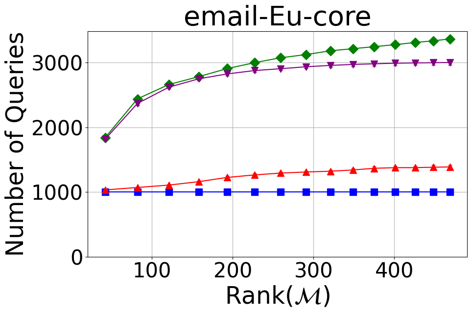
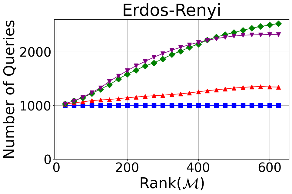
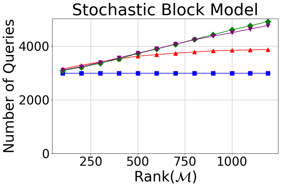
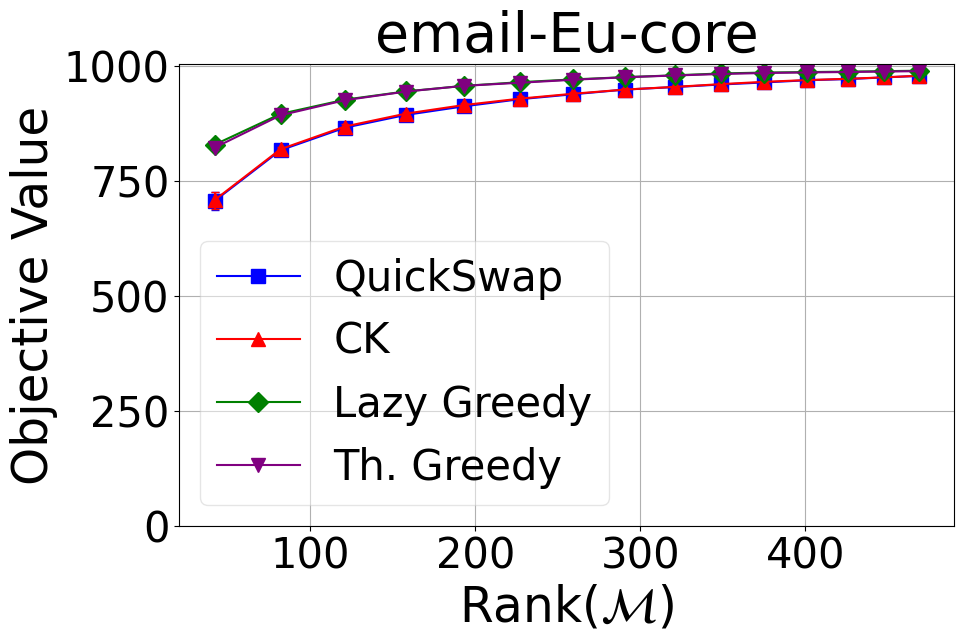
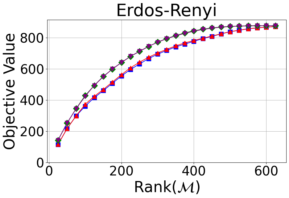
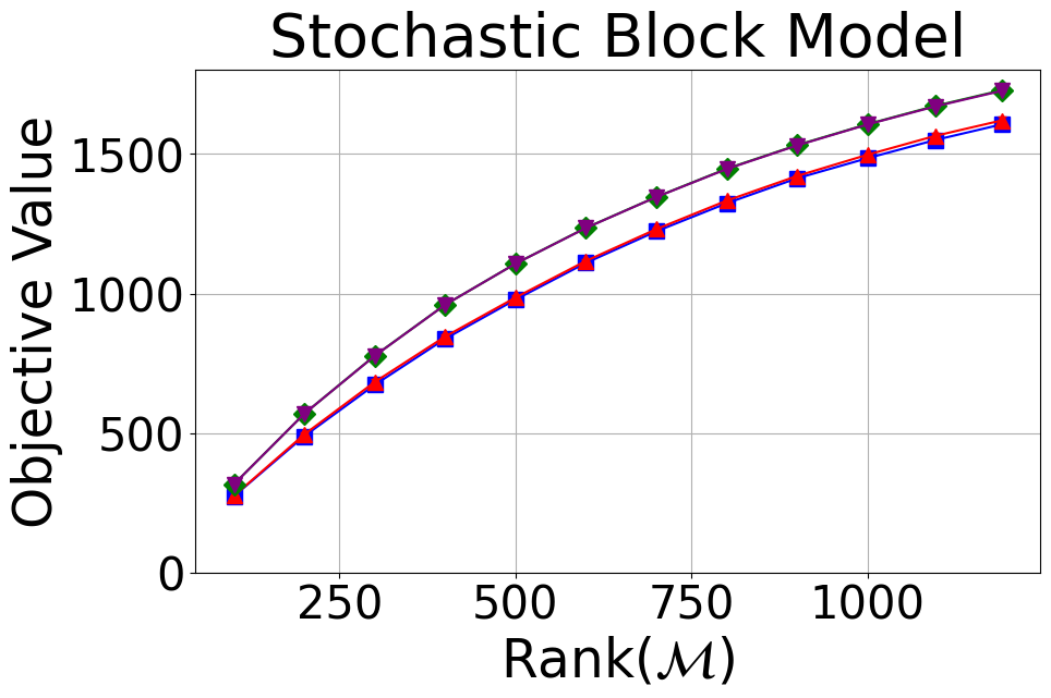
Figure 1: The numbers of queries and objective values achieves by the four algorithms for MSM as a function of rank of the matroid. For the objective value plots, lazy greedy and threshold greedy achieve nearly identical objective values and their lines overlap. For the same reason, the lines for QuickSwap and CK also overlap for these plots.

Problem instances.

We consider instances of influence maximization subject to a partition matroid constraint on various graphs, similarly to the experiment setting in [5] and [13]. In particular, given some graph $G=(V,E)$, we measure influence as defined by the coverage function $f:2^{V}\rightarrow Z_{\geq 0}$ where $f(S)=|\{v\in V\,|\,\exists s\in S\text{ such that }(s,v)\in E\}|$. The three graphs over $n$ nodes and $m$ edges, and the partition matroids, are as follows (additional details in Appendix A):

• email-Eu-core: The SNAP network email-Eu-core [25] is a real-world directed social network with $n=1005$ and $m=25571$. The dataset also includes which of 41 possible departments each individual belongs to, with these sets forming the parts of the partition matroid.

• Erdos-Renyi: An Erdos-Renyi graph with $n=1000$ and edge-formation probability $p=\frac{1}{500}$. The partition is generated by assigning each node to one of $20$ parts uniformly at random.

• Stochastic Block Model: A randomly generated graph according to the stochastic block model (SBM) with $100$ communities that have uniformly random size between $10$ and $50$. The parts of the partition matroid are the 100 sets corresponding to these 100 communities.

Results.

For the objective value plots, lazy greedy and threshold greedy achieve nearly identical objective values and their lines overlap. For the same reason, the lines for QuickSwap and CK also overlap for these plots. As shown in Figure 1, QuickSwap always achieves the least number of queries of all algorithms tested (exactly $n$ in each instance). QuickSwap significantly improves on the number of queries compared to lazy greedy and threshold greedy, at a small loss in objective value. More precisely, QuickSwap always achieves at least 80%, and often significantly over 90%, of the objective value achieved by lazy greedy and threshold greedy. For the performance of QuickSwap against the CK algorithm, it always requires fewer queries (and typically 20 to 30% less for larger size constraints), while simultaneously achieving nearly identical objective values.

5 Conclusion

In this work, we provide a deterministic algorithm for MSM that achieves a constant approximation factor with exactly $n$ queries to the oracle for the submodular function. However, our ratio of $1/4$ is smaller than the optimal ratio of $1-1/e\approx 0.63$. An interesting question for future work is what is the best ratio achievable with $\mathcal{O}(n)$ queries – in particular, is it possible to achieve the $1-1/e$ ratio, or even the $1/2$ ratio of the greedy algorithm with linear query complexity? For the general, non-monotone problem GSM, similar questions apply. We provided the first constant-factor approximation with linear query complexity, but our approximation ratio of $\approx 0.085$ in this setting is far from the best known ratio of $0.401$ [7] in polynomial time.

Furthermore, in this paper we consider the value query model, and measure the efficiency of an algorithm by the number of queries made to the oracle. We do not consider other metrics, such as the number of arithmetic operations or independence queries to the matroid. While computing the value of $f$ typically dominates other parts of the computation in most applications of submodular optimization, this may not hold true for all applications. In addition, there are other aspects related to computational efficiency, such as the ability to optimize marginal gain queries. We believe our algorithm would be able to be highly optimized in such settings (as it only queries the marginal gain into a nested sequence of sets), but we did not attempt to evaluate this explicitly.

Appendix A Additional details about experimental setup

A.1 Additional details about the algorithms

Below we provide specific details regarding the implementations of our algorithms from the experimental setup, including how queries were counted as well as specific data structures and parameter settings used. Note that in all implementations, once a given set has been queried for its value and causes the query count to increase by 1, this set will never again contribute to an increase in query count for any repeated computation which requires its evaluation.

• QuickSwap: Implemented exactly as in Algorithm 1, with $\beta=1$.

• CK Algorithm: This algorithm by Chakrabarti and Kale [10] takes one pass through the ground set and maintains a feasible set through the following swapping logic. Each element is assigned a weight (which requires at most two queries to the oracle), and the feasible solution is updated via appealing to an algorithm of Ashwinkumar [1] for maximum (modular) weight independent set. In particular, the weight of an element $e$ at the time of its consideration is set as its marginal contribution to the current maintained feasible, and it maintains this weight assignment throughout the entire duration of the algorithm. If $e$ can be added to this feasible set while maintaining its feasibility, it is added. Otherwise, it checks to see if the weight of $e$ is at least twice the weight of the minimum-weight element in the current feasible set which can be swapped with $e$ while maintaining feasibility. If this is the case, the swap occurs, and otherwise $e$ is not added to the feasible set and it remains unchanged.

• Lazy Greedy: Initially, the value of each singelton set is queried, with these corresponding values being assigned as priorties to each corresponding element and pushed onto a max heap. The initial query count is thus set to $n$, and the top element of the heap is popped and added to the maintained independent set $S$. From this point on, in each iteration the top element $e$ is popped from the max heap and we check if $e$ is the same element that was most recently popped. If so, we add $e$ to $S$. Otherwise, we check if $S+e$ is independent. If so, $e$ is pushed back onto the heap with priority $f(e|S)$ (and the query count is incremented by 1, not 2, as $f(S)$ must have already been queried as this computation only requires we newly query $f(S+e)$), and otherwise $e$ is not pushed onto the heap nor queried for its marginal contribution and we continue. This process continues until the heap is empty, i.e. no new element can be added to $S$ while maintaining its independence.

• Threshold Greedy: Two instances of threshold greedy were tested, for corresponding values of $\varepsilon=0.1$ and $\varepsilon=\frac{1}{6}$. The value $\varepsilon=\frac{1}{6}$ was chosen as it corresponds to the threshold value guaranteeing a $\frac{1}{4}$-approximation ratio. The value $\varepsilon=0.1$ was chosen to improve solution quality, at the potential risk of increasing the number of required queries. As these two parameters led to nearly identical performance (visually indistinguishable behavior in the plots), the version of threshold greedy implemented in this paper is for $\varepsilon=\frac{1}{6}$. Our implementation is based on that of Algorithm 1 in Badanidiyuru and Vondrák [3], which is a threshold greedy algorithm for monotone submodular maximization subject to a cardinality constraint, except that in each instance the algorithm checks $S+e$ satisfies the cardinality constraint we instead check that the appropriate matroid constraint is satisfied, and the lower-limit on the threshold at which point we stop checking is set to $\frac{\varepsilon}{r}$ where $r$ is the rank of the matroid. Furthermore, when we count queries, for each element we lazily store its last queried marginal contribution, so that it is only reevaluated should it be at least as large as the current threshold (as otherwise submodularity guarantees it must still be less than the current threshold).

A.2 Additional details about the problem instances

For each graph $G$, the partition matroid constraints considered are defined by a fixed partition of $V$ into sets $P_{1},\ldots,P_{m}$ (whose union is $V$ and pairwise intersection is always empty) and corresponding nonnegative integers $k_{1},\ldots,k_{m}$ such that any set $I\subset V$ is independent if and only if $I\cap P_{i}\leq k_{i}$ for each $i$. For our experiments, we consider partition matroids with fixed size constraints, i.e. such that $k_{1}=\ldots=k_{m}$. For the instances, we consider partition matroids with positive integer size constraints from $1$ up to $15$, $25$ and $12$ respectively. The three graphs and the partition matroids are as follows:

• email-Eu-core: The SNAP network email-Eu-core [25] representing email exchanges between members of a large European research institution, where each node corresponds to a member of the institution and each edge points from email senders to their recipients. The dataset also includes which of 41 possible departments each individual belongs to, with these sets forming the parts of the partition underlying each partition matroid considered. There are 1005 nodes and 25571 edges in this graph. Note that this dataset is released under the BSD license on SNAP, meaning it is free for both academic and commercial use.

• Erdos-Renyi: An Erdos-Renyi graph of 1000 nodes with edge-formation probability $p=\frac{1}{500}$, and a partition generated by assigning each node to one of 20 parts uniformly at random.

• Stochastic Block Model: A randomly generated graph according to the stochastic block model (SBM), with 100 communities set to have sizes chosen uniformly random from 10 to 50 inclusive, with edge formation probability of 0 between nodes in different communities and $\frac{1}{30}$ between nodes in the same community. The parts of the underlying partition are the 100 sets corresponding to these 100 communities.

A.3 Mean ± standard deviation tables

As each data point plotted corresponds to a mean of 5 trials, the corresponding standard deviations were computed. However, each was too small to be visible on the plots, with most standard deviations being less than 1% of their corresponding mean. Thus, these values, along with the exact value of the mean, are provided in Tables 1, 2, 3, 4, 5 and 6.

A.4 Compute resources

All code was run in a Jupyter Notebook, and took no more than 3 hours total to run on a standard Mac with an M1 chip.

Table 1: Mean ± Standard Deviation of Queries on email-Eu-core

Matroid Rank QuickSwap CK Lazy Greedy Threshold Greedy 42 1005.0 ± 0.0 1032.4 ± 3.1 1840.0 ± 0.0 1815.4 ± 15.5 82 1005.0 ± 0.0 1070.0 ± 7.8 2439.0 ± 0.0 2368.0 ± 33.4 121 1005.0 ± 0.0 1107.0 ± 12.0 2661.6 ± 0.5 2620.4 ± 25.6 158 1005.0 ± 0.0 1159.8 ± 15.7 2782.8 ± 1.2 2749.4 ± 25.0 193 1005.0 ± 0.0 1225.2 ± 29.0 2907.2 ± 0.7 2824.4 ± 29.5 227 1005.0 ± 0.0 1264.0 ± 21.7 2998.8 ± 1.3 2877.0 ± 26.6 259 1005.0 ± 0.0 1292.4 ± 22.1 3074.4 ± 1.6 2905.2 ± 26.5 291 1005.0 ± 0.0 1309.4 ± 16.5 3124.0 ± 1.1 2935.6 ± 26.5 321 1005.0 ± 0.0 1321.6 ± 18.0 3182.8 ± 0.7 2956.8 ± 30.6 349 1005.0 ± 0.0 1341.0 ± 21.3 3215.2 ± 2.0 2971.8 ± 32.6 375 1005.0 ± 0.0 1366.4 ± 24.7 3245.8 ± 0.7 2981.2 ± 30.9 401 1005.0 ± 0.0 1376.2 ± 24.4 3277.2 ± 1.3 2990.4 ± 32.5 426 1005.0 ± 0.0 1376.6 ± 28.2 3311.2 ± 0.4 2995.0 ± 34.1 448 1005.0 ± 0.0 1382.8 ± 30.7 3336.2 ± 0.4 2998.0 ± 34.2 469 1005.0 ± 0.0 1388.0 ± 28.3 3366.2 ± 2.0 3001.8 ± 35.8

Table 2: Mean ± Standard Deviation of Queries on ER

Matroid Rank QuickSwap CK Lazy Greedy Threshold Greedy 25 1000.0 ± 0.0 1026.6 ± 2.7 1032.4 ± 1.9 1033.0 ± 2.6 50 1000.0 ± 0.0 1049.2 ± 3.6 1084.8 ± 3.4 1085.8 ± 4.1 75 1000.0 ± 0.0 1067.8 ± 7.0 1145.8 ± 5.2 1152.6 ± 6.4 100 1000.0 ± 0.0 1090.2 ± 8.0 1222.2 ± 7.9 1238.8 ± 14.6 125 1000.0 ± 0.0 1102.6 ± 6.9 1304.2 ± 5.8 1329.0 ± 10.4 150 1000.0 ± 0.0 1112.0 ± 8.2 1386.0 ± 9.6 1449.0 ± 14.1 175 1000.0 ± 0.0 1127.0 ± 5.8 1493.2 ± 7.0 1551.0 ± 15.7 200 1000.0 ± 0.0 1143.4 ± 4.5 1584.0 ± 12.1 1648.4 ± 14.4 225 1000.0 ± 0.0 1157.4 ± 1.9 1658.6 ± 16.7 1739.6 ± 11.0 250 1000.0 ± 0.0 1171.6 ± 6.2 1736.8 ± 9.9 1820.0 ± 9.8 275 1000.0 ± 0.0 1181.4 ± 8.1 1794.6 ± 12.4 1899.6 ± 10.5 300 1000.0 ± 0.0 1191.4 ± 9.0 1868.2 ± 15.7 1967.0 ± 13.3 325 1000.0 ± 0.0 1204.6 ± 7.5 1948.4 ± 10.0 2030.2 ± 14.0 350 1000.0 ± 0.0 1216.8 ± 6.6 2011.8 ± 14.2 2083.0 ± 9.1 375 1000.0 ± 0.0 1233.0 ± 7.8 2084.4 ± 7.1 2133.2 ± 10.9 400 1000.0 ± 0.0 1256.8 ± 8.7 2144.2 ± 11.9 2175.6 ± 15.6 425 1000.0 ± 0.0 1274.4 ± 10.3 2218.6 ± 14.4 2215.6 ± 15.3 450 1000.0 ± 0.0 1291.4 ± 19.4 2275.0 ± 11.4 2245.8 ± 13.4 475 1000.0 ± 0.0 1308.0 ± 19.7 2319.6 ± 10.7 2271.4 ± 6.7 500 1000.0 ± 0.0 1325.4 ± 17.0 2359.4 ± 12.7 2293.4 ± 7.6 525 1000.0 ± 0.0 1336.0 ± 13.0 2401.8 ± 9.3 2308.6 ± 5.5 550 1000.0 ± 0.0 1347.4 ± 13.2 2439.8 ± 6.8 2315.4 ± 5.3 575 1000.0 ± 0.0 1353.8 ± 11.6 2472.2 ± 3.3 2319.4 ± 5.0 600 1000.0 ± 0.0 1345.8 ± 12.0 2500.2 ± 4.3 2323.0 ± 3.4 625 1000.0 ± 0.0 1342.8 ± 10.2 2525.2 ± 4.3 2324.0 ± 3.6

Table 3: Mean ± Standard Deviation of Queries on SBM

Matroid Rank QuickSwap CK Lazy Greedy Threshold Greedy 100 2992.0 ± 0.0 3150.0 ± 8.9 3091.0 ± 0.0 3110.0 ± 0.0 200 2992.0 ± 0.0 3287.0 ± 16.2 3210.8 ± 2.5 3232.4 ± 1.4 300 2992.0 ± 0.0 3410.8 ± 7.6 3359.4 ± 2.0 3394.2 ± 3.5 400 2992.0 ± 0.0 3525.2 ± 13.1 3524.8 ± 8.1 3563.4 ± 6.6 500 2992.0 ± 0.0 3625.2 ± 25.0 3726.0 ± 6.3 3736.8 ± 13.1 600 2992.0 ± 0.0 3684.0 ± 33.0 3892.6 ± 6.0 3902.6 ± 7.5 700 2992.0 ± 0.0 3733.6 ± 29.5 4071.2 ± 4.1 4071.8 ± 5.3 800 2992.0 ± 0.0 3781.6 ± 25.0 4249.2 ± 13.5 4236.6 ± 8.5 900 2992.0 ± 0.0 3823.0 ± 23.7 4428.0 ± 19.0 4373.6 ± 15.0 1000 2992.0 ± 0.0 3842.8 ± 14.7 4606.6 ± 15.7 4501.8 ± 11.8 1096 2992.0 ± 0.0 3858.8 ± 11.1 4757.0 ± 12.4 4636.0 ± 11.4 1191 2992.0 ± 0.0 3873.2 ± 8.6 4919.2 ± 10.1 4766.8 ± 13.6

Table 4: Mean ± Standard Deviation of Objective Values on email-Eu-core

Matroid Rank QuickSwap CK Lazy Greedy Threshold Greedy 42 706.6 ± 20.5 708.4 ± 18.7 829.0 ± 0.0 822.4 ± 4.5 82 817.0 ± 6.1 819.2 ± 4.9 896.0 ± 0.0 893.0 ± 1.3 121 866.0 ± 4.2 868.6 ± 4.4 927.0 ± 0.0 925.8 ± 1.7 158 893.8 ± 2.5 896.6 ± 3.1 945.0 ± 0.0 944.6 ± 1.4 193 912.4 ± 3.8 915.2 ± 4.8 957.0 ± 0.0 957.0 ± 0.6 227 928.0 ± 5.4 929.2 ± 6.4 965.0 ± 0.0 963.8 ± 1.5 259 938.6 ± 2.9 939.8 ± 4.0 971.0 ± 0.0 970.2 ± 1.0 291 949.0 ± 2.9 949.0 ± 3.0 976.0 ± 0.0 975.8 ± 1.7 321 954.4 ± 3.1 954.8 ± 2.9 980.0 ± 0.0 979.6 ± 2.1 349 960.0 ± 3.1 960.8 ± 2.9 984.0 ± 0.0 982.8 ± 1.7 375 964.4 ± 4.1 965.8 ± 4.3 986.0 ± 0.0 985.0 ± 1.1 401 969.2 ± 3.9 969.6 ± 4.2 987.0 ± 0.0 986.2 ± 0.4 426 971.8 ± 2.6 972.4 ± 3.3 988.0 ± 0.0 987.2 ± 0.7 448 975.4 ± 2.8 975.6 ± 2.9 989.0 ± 0.0 988.2 ± 0.7 469 978.8 ± 2.2 979.0 ± 2.3 990.0 ± 0.0 989.0 ± 0.9

Table 5: Mean ± Standard Deviation of Objective Values on ER

Matroid Rank QuickSwap CK Lazy Greedy Threshold Greedy 25 114.8 ± 1.9 116.0 ± 2.8 142.6 ± 1.0 142.4 ± 1.0 50 216.8 ± 3.8 216.2 ± 3.9 251.8 ± 1.2 253.0 ± 0.6 75 297.8 ± 3.1 298.6 ± 3.8 345.0 ± 1.1 344.0 ± 1.7 100 360.6 ± 5.7 372.2 ± 9.0 428.2 ± 0.4 423.8 ± 1.0 125 414.6 ± 2.8 423.4 ± 2.7 492.8 ± 1.7 493.2 ± 2.0 150 459.8 ± 7.5 467.4 ± 6.9 551.0 ± 4.4 549.0 ± 3.1 175 506.6 ± 5.4 515.0 ± 2.6 597.2 ± 2.5 598.6 ± 2.8 200 553.8 ± 6.5 562.0 ± 5.9 640.0 ± 2.3 639.8 ± 3.2 225 595.2 ± 5.8 606.0 ± 3.6 678.8 ± 2.1 679.4 ± 2.4 250 630.8 ± 6.0 642.0 ± 4.0 711.2 ± 2.0 712.4 ± 1.9 275 665.0 ± 5.9 673.6 ± 3.0 742.6 ± 1.9 743.2 ± 1.0 300 693.4 ± 4.4 701.0 ± 3.7 770.8 ± 1.9 769.6 ± 1.4 325 717.2 ± 4.2 724.2 ± 6.5 793.4 ± 2.1 792.4 ± 1.4 350 740.2 ± 7.7 746.6 ± 8.8 813.0 ± 3.8 811.0 ± 2.6 375 758.2 ± 8.2 765.8 ± 7.4 829.6 ± 3.3 826.6 ± 4.3 400 775.8 ± 6.0 780.8 ± 3.2 843.2 ± 3.2 840.4 ± 4.0 425 793.2 ± 5.2 795.6 ± 4.4 853.6 ± 1.6 851.6 ± 3.7 450 807.4 ± 4.8 809.6 ± 3.9 861.6 ± 1.5 860.0 ± 3.0 475 823.0 ± 3.9 824.0 ± 3.9 867.6 ± 2.1 866.4 ± 3.1 500 837.2 ± 3.7 837.6 ± 3.1 871.4 ± 1.0 870.6 ± 2.3 525 846.8 ± 2.0 847.0 ± 1.9 873.6 ± 0.5 873.0 ± 2.1 550 855.8 ± 2.6 856.4 ± 2.7 875.4 ± 0.5 874.2 ± 1.5 575 861.6 ± 2.8 862.0 ± 2.6 876.0 ± 0.0 875.4 ± 0.8 600 866.4 ± 1.5 866.6 ± 1.4 876.0 ± 0.0 876.0 ± 0.0 625 870.4 ± 1.4 870.6 ± 1.5 876.0 ± 0.0 876.0 ± 0.0

Table 6: Mean ± Standard Deviation of Objective Values on SBM

Matroid Rank QuickSwap CK Lazy Greedy Threshold Greedy 100 273.2 ± 3.5 274.4 ± 3.0 316.0 ± 0.0 316.0 ± 0.0 200 488.6 ± 8.5 494.8 ± 7.2 569.0 ± 0.0 569.0 ± 0.0 300 672.4 ± 9.8 682.6 ± 11.9 777.0 ± 0.0 776.2 ± 0.4 400 837.4 ± 4.6 845.4 ± 9.0 959.6 ± 1.0 959.4 ± 1.0 500 978.0 ± 8.2 985.4 ± 9.1 1107.0 ± 0.9 1106.8 ± 1.3 600 1109.6 ± 9.5 1116.6 ± 8.3 1235.4 ± 1.0 1234.6 ± 1.9 700 1222.8 ± 6.5 1230.6 ± 6.8 1346.2 ± 1.2 1345.6 ± 2.2 800 1323.4 ± 4.5 1332.8 ± 2.8 1447.4 ± 1.2 1446.0 ± 2.4 900 1413.0 ± 3.0 1421.2 ± 3.2 1532.0 ± 0.6 1530.6 ± 2.3 1000 1485.0 ± 8.3 1497.4 ± 5.3 1607.0 ± 1.1 1605.8 ± 2.3 1096 1550.0 ± 10.3 1564.8 ± 10.4 1672.4 ± 1.6 1670.4 ± 1.7 1191 1606.4 ± 10.4 1620.6 ± 13.3 1728.8 ± 1.5 1726.6 ± 1.6

References

- Ashwinkumar [2011] B. V. Ashwinkumar. Buyback Problem - Approximate matroid intersection with cancellation costs. In Proceedings of the 38th International Colloquium Conference on Automata, Languages and Programming, volume 6755, pages 379–390, 2011. doi: 10.1007/978-3-642-22006-7_32.
- Badanidiyuru and Vondrák [2014] Ashwinkumar Badanidiyuru and Jan Vondrák. Fast algorithms for maximizing submodular functions. In Proceedings of the Twenty-Fifth Annual ACM-SIAM Symposium on Discrete Algorithms, pages 1497–1514. Society for Industrial and Applied Mathematics, January 2014. ISBN 978-1-61197-338-9 978-1-61197-340-2. doi: 10.1137/1.9781611973402.110.
- Badanidiyuru and Vondrák [2014] Ashwinkumar Badanidiyuru and Jan Vondrák. Fast algorithms for maximizing submodular functions, pages 1497–1514. 01 2014. ISBN 978-1-61197-338-9. doi: 10.1137/1.9781611973402.110.
- Badanidiyuru et al. [2014] Ashwinkumar Badanidiyuru, Baharan Mirzasoleiman, Amin Karbasi, and Andreas Krause. Streaming submodular maximization: Massive data summarization on the fly. In Proceedings of the 20th ACM SIGKDD international conference on Knowledge discovery and data mining, pages 671–680, 2014.
- Balkanski et al. [2018] Eric Balkanski, Adam Breuer, and Yaron Singer. Non-monotone submodular maximization in exponentially fewer iterations. In Advances in Neural Information Processing Systems 31 (NeurIPS 2018), 2018.
- Breuer et al. [2020] Adam Breuer, Eric Balkanski, and Yaron Singer. The FAST Algorithm for Submodular Maximization. In Proceedings of the 37th International Conference on Machine Learning, pages 1134–1143. PMLR, November 2020.
- Buchbinder and Feldman [2023] Niv Buchbinder and Moran Feldman. Constrained Submodular Maximization via New Bounds for DR-Submodular Functions, arXiv, November 2023.
- Buchbinder et al. [2015] Niv Buchbinder, Moran Feldman, and Roy Schwartz. Comparing Apples and Oranges: Query Tradeoff in Submodular Maximization. In ACM-SIAM Symposium on Discrete Algorithms (SODA), 2015. doi: 10.1137/1.9781611973730.77.
- Calinescu et al. [2011] Gruia Calinescu, Chandra Chekuri, Martin Pal, and Jan Vondrák. Maximizing a monotone submodular function subject to a matroid constraint. SIAM Journal on Computing, 40(6):1740–1766, 2011.
- Chakrabarti and Kale [2015] Amit Chakrabarti and Sagar Kale. Submodular maximization meets streaming: Matchings, matroids, and more. Mathematical Programming, 154(1):225–247, December 2015. ISSN 1436-4646. doi: 10.1007/s10107-015-0900-7.
- Chekuri et al. [2015] Chandra Chekuri, Shalmoli Gupta, and Kent Quanrud. Streaming Algorithms for Submodular Function Maximization. In International Colloquium on Automata, Languages, and Programming (ICALP), 2015.
- Das and Kempe [2011] Abhimanyu Das and David Kempe. Submodular meets spectral: Greedy algorithms for subset selection, sparse approximation and dictionary selection. In Proc. 28th Int. Conf. on Machine Learning (ICML’11), pages 1057–1064, 2011.
- Dütting et al. [2022] Paul Dütting, Federico Fusco, Silvio Lattanzi, Ashkan Norouzi-Fard, and Morteza Zadimoghaddam. Deletion robust submodular maximization over matroids. In Proceedings of the 39th International Conference on Machine Learning, volume 162 of Proceedings of Machine Learning Research, pages 5671–5693. PMLR, 2022.
- Ene and Nguyen [2019] Alina Ene and Huy L. Nguyen. A Nearly-linear Time Algorithm for Submodular Maximization with a Knapsack Constraint. In ICALP, pages 1–24, 2019.
- Feldman et al. [2018] Moran Feldman, Amin Karbasi, and Ehsan Kazemi. Do Less, Get More: Streaming Submodular Maximization with Subsampling. In Advances in Neural Information Processing Systems, volume 31. Curran Associates, Inc., 2018.
- Fisher et al. [1978] Marshall L Fisher, George L Nemhauser, and Laurence A Wolsey. An analysis of approximations for maximizing submodular set functions—II. Springer, 1978.
- [17] Michel Goemans. Matroid optimization notes. https://math.mit.edu/~goemans/18433S13/matroid-notes.pdf.
- Han et al. [2020] Kai Han, Zongmai Cao, Shuang Cui, and Benwei Wu. Deterministic Approximation for Submodular Maximization over a Matroid in Nearly Linear Time. In NeurIPS, pages 1–12, 2020.
- Kempe et al. [2003] David Kempe, Jon Kleinberg, and Éva Tardos. Maximizing the spread of influence through a social network. In Proceedings of the ninth ACM SIGKDD international conference on Knowledge discovery and data mining, pages 137–146, 2003.
- Kobayashi and Terao [2024] Yusuke Kobayashi and Tatsuya Terao. Subquadratic Submodular Maximization with a General Matroid Constraint. In arXiv:2405.00359. arXiv, May 2024.
- Kuhnle [2019] Alan Kuhnle. Interlaced Greedy Algorithm for Maximization of Submodular Functions in Nearly Linear Time. In Advances in Neural Information Processing Systems, volume 32. Curran Associates, Inc., 2019.
- Kuhnle [2021] Alan Kuhnle. Quick Streaming Algorithms for Maximization of Monotone Submodular Functions in Linear Time. In Artificial Intelligence and Statistics (AISTATS), 2021.
- Kupfer et al. [2020] Ron Kupfer, Sharon Qian, Eric Balkanski, and Yaron Singer. The adaptive complexity of maximizing a gross substitutes valuation. Advances in Neural Information Processing Systems, 33:19817–19827, 2020.
- Lee et al. [2009] Jon Lee, Vahab S Mirrokni, Viswanath Nagarajan, and Maxim Sviridenko. Non-monotone submodular maximization under matroid and knapsack constraints. In Proceedings of the forty-first annual ACM symposium on Theory of computing, pages 323–332, 2009.
- Leskovec and Krevl [2014] Jure Leskovec and Andrej Krevl. Snap dataset: email-eu-core. https://snap.stanford.edu/data/email-Eu-core.html, Stanford Network Analysis Project (SNAP), 2014.
- Li et al. [2022] Wenxin Li, Moran Feldman, Ehsan Kazemi, and Amin Karbasi. Submodular Maximization in Clean Linear Time. Advances in Neural Information Processing Systems, 35:17473–17487, December 2022.
- Lin and Bilmes [2011] Hui Lin and Jeff Bilmes. A class of submodular functions for document summarization. In Proceedings of the 49th annual meeting of the association for computational linguistics: human language technologies, pages 510–520, 2011.
- Minoux [1978] Michel Minoux. Accelerated greedy algorithms for maximizing submodular set functions. In J. Stoer, editor, Optimization Techniques, pages 234–243, Berlin, Heidelberg, 1978. Springer Berlin Heidelberg.
- Mirzasoleiman et al. [2015] Baharan Mirzasoleiman, Ashwinkumar Badanidiyuru, Amin Karbasi, Jan Vondrak, and Andreas Krause. Lazier Than Lazy Greedy. In AAAI Conference on Artificial Intelligence (AAAI), 2015. ISBN 978-1-57735-701-8.
- Nemhauser and Wolsey [1978] George L Nemhauser and Laurence A Wolsey. Best algorithms for approximating the maximum of a submodular set function. Mathematics of operations research, 3(3):177–188, 1978.
- Norouzi-Fard et al. [2018] Ashkan Norouzi-Fard, Jakub Tarnawski, Slobodan Mitrovic, Amir Zandieh, Aidasadat Mousavifar, and Ola Svensson. Beyond 1/2-approximation for submodular maximization on massive data streams. In International Conference on Machine Learning, pages 3829–3838. PMLR, 2018.