${\sf solar}$: A solar thermal power plant simulator for blackbox optimization benchmarking

Abstract: This work introduces ${\sf solar,}$ a collection of ten optimization problem instances for benchmarking blackbox optimization solvers. The instances present different design aspects of a concentrated solar power plant simulated by blackbox numerical models. The type of variables (discrete or continuous), dimensionality, and number and types of constraints (including hidden constraints) differ across instances. Some are deterministic, others are stochastic with possibilities to execute several replications to control stochasticity. Most instances offer variable fidelity surrogates, two are biobjective and one is unconstrained. The solar plant model takes into account various subsystems: a heliostats field, a central cavity receiver (the receiver), a molten salt thermal energy storage, a steam generator and an idealized power block. Several numerical methods are implemented throughout the ${\sf solar}$ code and most of the executions are time-consuming. Great care was applied to guarantee reproducibility across platforms. The ${\sf solar}$ tool encompasses most of the characteristics that can be found in industrial and real-life blackbox optimization problems, all in an open-source and stand-alone code.

Keywords: Blackbox optimization (BBO), Derivative-free optimization (DFO), Benchmark problem, Concentrated solar power (CSP), Solar thermal power.

AMS subject classifications: 90-04, 90-10, 90C56.

1 Introduction

Blackbox optimization (BBO) refers to optimization problems where the objective or constraint functions are not explicitly known or easily computable. The term blackbox refers to the fact that output values can only be obtained via querying the function at the corresponding input points. These problems arise in various fields, including engineering design, machine learning, finance and operations research. An introduction to BBO is found in the textbook [10], a survey on methodology and software appears in [28], a survey on direct-search methods is proposed in [44] and hundreds of applications are presented in [4].

The challenge in BBO lies in the lack of knowledge about the underlying functions. Since the internal structure is unknown, traditional optimization methods that rely on explicit mathematical expressions or gradient information cannot be directly applied. Instead, algorithmic techniques leverage sampling and exploration to iteratively search the solution space, probing the blackbox for evaluations at different points and using the obtained information to guide the search towards an optimal solution.

1.1 Inherent difficulties in BBO

BBO problems introduce several complexities and considerations. First, multiple types of variables might be available: some may be continuous, some discrete and some may even be categorical, i.e., variables which do not satisfy any ordering properties. In addition, some variables may have an impact on the dimension of the problems. Terminology for such variables is proposed in [9]. Second, the evaluation of the functions can be computationally expensive, limiting the number of function evaluations that can be performed. Therefore, an optimization algorithm needs to strike a balance between exploration and exploitation to efficiently find good solutions. Third, BBO problems often involve noisy or stochastic functions, where the output values may vary even for the same input. This necessitates the use of techniques that can handle noise and uncertainty. Fourth, in many real applications, the computer simulation used to compute the functions may unexpectedly fail to return valid output. For example, when evaluating a vibration measure of a helicopter rotor blade, approximately 60% of the simulation calls fail to return a value [20, 21]. These types of constraints are known as hidden constraints [24]. Some constraints may also return Boolean values, making it difficult for models to approximate them. Finally, there are situations where one wishes to simultaneously optimize more than one objective function. In this case, one does not wish to find a single solution, but one wishes to obtain a set of non-dominated solutions [13, 18, 27].

1.2 Challenges in BBO benchmarking

Performance [29] and data [52] profiles are now the standard tools for benchmarking derivative-free algorithms. They allow to agglomerate several optimization runs in simple-to-visualize graphs, and are flexible enough to account for blackbox evaluations. They can also easily be generalized to the constrained and multiobjective cases. Good benchmarking practices are exposed in [10, 16]. Accuracy profiles are a related variant described in [10]. The COCO suite [36] also provides useful benchmarking tools. For examples of recent benchmarking studies, see [53, 54].

Many engineering optimization problems rely on proprietary models and cannot be freely shared with the academic community that develops optimization methods. As a consequence, the performance of BBO methods is often assessed on artificial analytic test problems such as the Rosenbrock banana function [55], the Hock and Schittkowski collection [38] or the problems from Moré and Wild [52]. All of these problems are of crucial importance to nonlinear and derivative-free optimization, but are not representative of difficulties encountered in real BBO applications, in which the objective and constraint functions are not known analytically [10]. A special issue of Optimization and Engineering [11] is dedicated to such problems. The objective of the present work is to introduce a collection of optimization problems as benchmarks for the development of BBO methods. The collection is developed from a mechanical engineering perspective and is closer to the problems solved in practice. Other realistic BBO problems are publicly available. For example, [33] compares derivative-free optimization methods using a set of groundwater supply and hydraulic capture problems. A styrene engineering production problem is proposed in [7], and [2, 42] study the optimization of the number and composition of heat intercepts in a load-bearing thermal insulation system. A pump-and-treat groundwater remediation problem from the Montana Lockwood Solvent Groundwater Plume Site is introduced in [51] using the Bluebird simulator [26].

Taken separately, these examples offer desirable characteristics for benchmarking BBO such as multifidelity, stochasticity, multiobjective and hidden constraints. In fact, it seems that no work exhibits a realistic application specifically developed for BBO benchmarking. ${\sf solar}$ is the first realistic blackbox that gathers all of these characteristics in a single family of instances. Various optimization of CSP plants are described in [25, 49, 50], but they do not provide benchmarking tools.

1.3 Contributions

The main contribution of this work is to provide a family of blackbox benchmarking optimization instances. The proposed blackbox gathers most of the desired characteristics of real-world problems, such as time-extensive evaluations, variable fidelity, stochasticity, surrogates, multiobjective, and several types of constraints, including hidden constraints.

The engineering models proposed within the blackbox simulates the operation of a concentrated solar power (CSP) tower plant with molten salt thermal energy storage. In this design, a large number of mirrors, or heliostats, reflects solar radiation on the receiver at the top of a tower. The heat collected from the concentrated solar flux is removed from the receiver by a stream of molten salt. Hot molten salt is then either used to feed thermal power to a conventional power block, or stored in an insulated tank for deferred use. The Thémis CSP power plant [30] (see Figure 1), in France, was the first built with this design. Gemasolar, in Spain, was the first CSP tower plant to produce electrical power on a “24/7” basis using molten salt thermal energy storage [23].

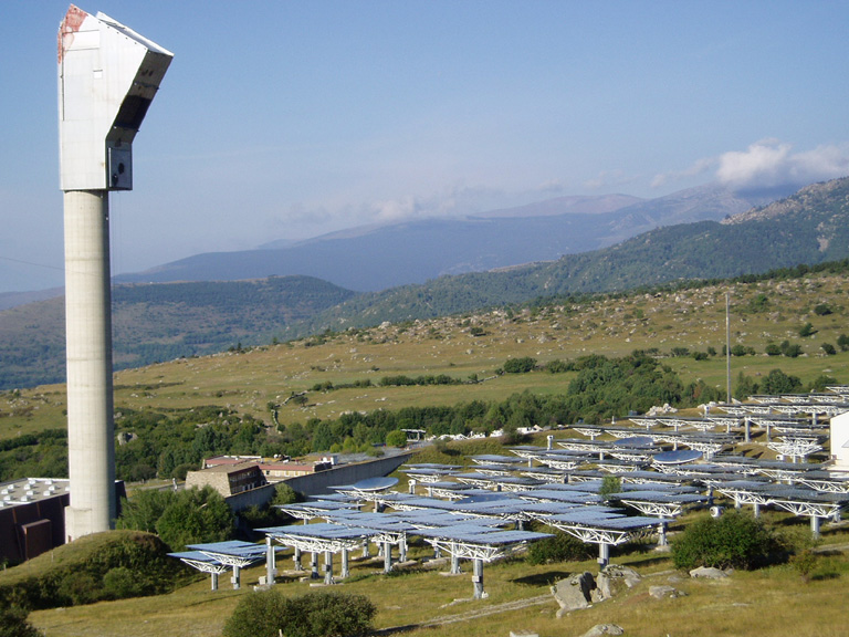
Figure 1: The Thémis CSP tower plant in Targasonne, France.
Source: https://commons.wikimedia.org/wiki/File:Themis$\_$2.jpg.

The source code of the models is freely available under the LGPL license at https://github.com/bbopt/solar, along with some starting points, best known values, and the logs provided by some solvers such as NOMAD [12, 45]. ${\sf solar}$ is written in standard C++, and compiles on most platforms and is guaranteed to reproduce the exact same outputs independently of the platform. It also provides variable-fidelity static surrogates, deterministic or stochastic outputs, and the control over its number of replications, leading to reduced variance in the output at the cost of more time-expansive simulations. The code is parametrized so that a total of 10 BBO problems instances with various complexity levels is provided. These instances are single- or bi-objective, involve between 5 and 29 integer, real or categorical variables, and implement between 5 and 17 binary, integer or continuous constraints. In addition, hidden constraints are present as some evaluations may fail to compute.

1.4 Organization

The paper is structured as follows: Section 2 provides a short literature review on solar plants, and a high-level description of the main components of the power plant model. The complete model description is available separately, in the MSc thesis [47]. Section 3 describes the collection of test problems from the point of view of BBO benchmarking. Section 4 describes the ${\sf solar}$ package, its many features, and provides illustrative examples of typical benchmarking situations. Concluding remarks follow.

2 Description of the solar thermal power plant simulator

This section gives a short literature review on CSP plants and introduces the technologies that are simulated when different instances are queried, as well as the mathematical/numerical models used to represent them.

2.1 A short literature review on solar plants

Solar energy has emerged as a pivotal solution to address challenges associated with fossil fuel depletion, environmental degradation, and climate change. Thermal energy, derived from solar radiation, represents a potentially abundant energy source. Harnessing and storing energy from solar radiation primarily involve two methods: photovoltaic and thermal energy storage.

Photovoltaics convert solar radiation into electrical energy, which can be used immediately or stored using batteries. When integrated into the grid, inverters are employed to convert direct current into alternating current. However, the intermittent and variable nature of solar radiation introduces substantial unpredictability into its utilization. Therefore, the development of efficient energy storage systems is imperative to fully realize its benefits. Thermal energy storage technologies entail the transfer of energy to a material, leading to an increase in its total enthalpy.This stored energy can be deployed as needed to meet grid power demands. Ultimately, the stored energy is transferred to a heat-transfer fluid, often water, using either sensible heat (heat transfer without a change in state) or latent heat interactions.

One example of sensible heat storage technology is the Solar Electric Station IX in California’s Mojave Desert, which utilizes a Phase Change Material (PCM). PCMs enable energy storage or release through a first-order phase transition, and the enthalpies of these transitions, known as latent heat, quantify the heat interactions. Four possible phase transformations can be used for heat storage: solid-solid, solid-liquid, solid-gas, and liquid-gas reactions. PCMs that undergo solid-liquid phase transitions offer the highest energy density variation, providing gigajoules of energy compared to kilojoules for liquid-gas transitions. Wei et al. [61] have reviewed the selection principles for PCMs, considering material properties like heat of transition, melting mechanism, thermal conductivity, heat capacity, volume change upon phase change, vapor pressure, reactivity, operating temperature constraints, and heat transfer equipment design.

Thermophysical properties are essential in PCM design. Numerous materials can serve as PCMs, covering a wide range [32, 40, 41, 56]. They are often categorized based on their chemical properties, with classifications for low-temperature thermal energy storage by Abhat [1] and for medium and high-temperature PCMs in [41]. In [35], a comprehensive analysis of the intricate interplay between thermophysical, thermal, economic, and corrosion properties identifies optimal PCMs for sustainable CSP plants. The study identified criteria including exceptional heat storage capacity, optimal thermal conductivity in solid and liquid phases, and high heat capacity per unit volume.

2.2 Introduction to the simulator

Several CSP subsystems are involved in the transformation of direct solar irradiation to electrical power. Table 1 details the quantities and notations used through this work. Note that these quantities do not necessarily correspond to the optimization variables described in Section 3.

Name	Quantity	Units
$D$	outer diameter	$\mathrm{m}$
$d$	inner diameter	$\mathrm{m}$
$H$	height	m
$L$	length	m
$P$	parasitic load	k$\mathrm{W}$
$Q$	heat transfer	k$\mathrm{W}$
$R$	radius	$\mathrm{m}$
$ST$	type of steam turbine	$-$
$t$	thickness	$\mathrm{m}$
$W$	width	$\mathrm{m}$
$\eta$	efficiency	$-$
$\theta$	angle	deg
$\tau$	transmissivity	$-$

Subscript	Definition
$\mathrm{baf}$	baffles
$\mathrm{bot}$	bottom
$\mathrm{cold}$	cold tank
$\mathrm{conv}$	convection
$\mathrm{cos}$	cosine effect
$\mathrm{hot}$	hot tank
$\mathrm{hf}$	heliostats field
$\mathrm{ms}$	molten salt
$\mathrm{pass}$	passes in steam generator
$\mathrm{rad}$	radiation
$\mathrm{rcv}$	receiver
$\mathrm{sg}$	steam generator
$\mathrm{sh}$	shell
$\mathrm{spl}$	spillage
$\mathrm{tank}$	tank ($\mathrm{hot}$ or $\mathrm{cold}$)
$\mathrm{tub}$	tubes
$\mathrm{trb}$	turbine
$\mathrm{twr}$	tower

Table 1: Notations for various quantities and signification of subscripts. Subscripts “$\mathrm{dry}$”, “$\mathrm{top}$” and “$\mathrm{wet}$” are obvious.

2.3 System dynamics

The plant is designed to transform heat recovered from concentrated sunlight into electrical power. Due to the Second Law of Thermodynamics and to non-idealities in each subsystem, part of the input heat is rejected during the process to the environment. Figure 2 provides an overview of the complete cycle. Losses due to non-idealities are not represented but are accounted for in all components except the steam generator

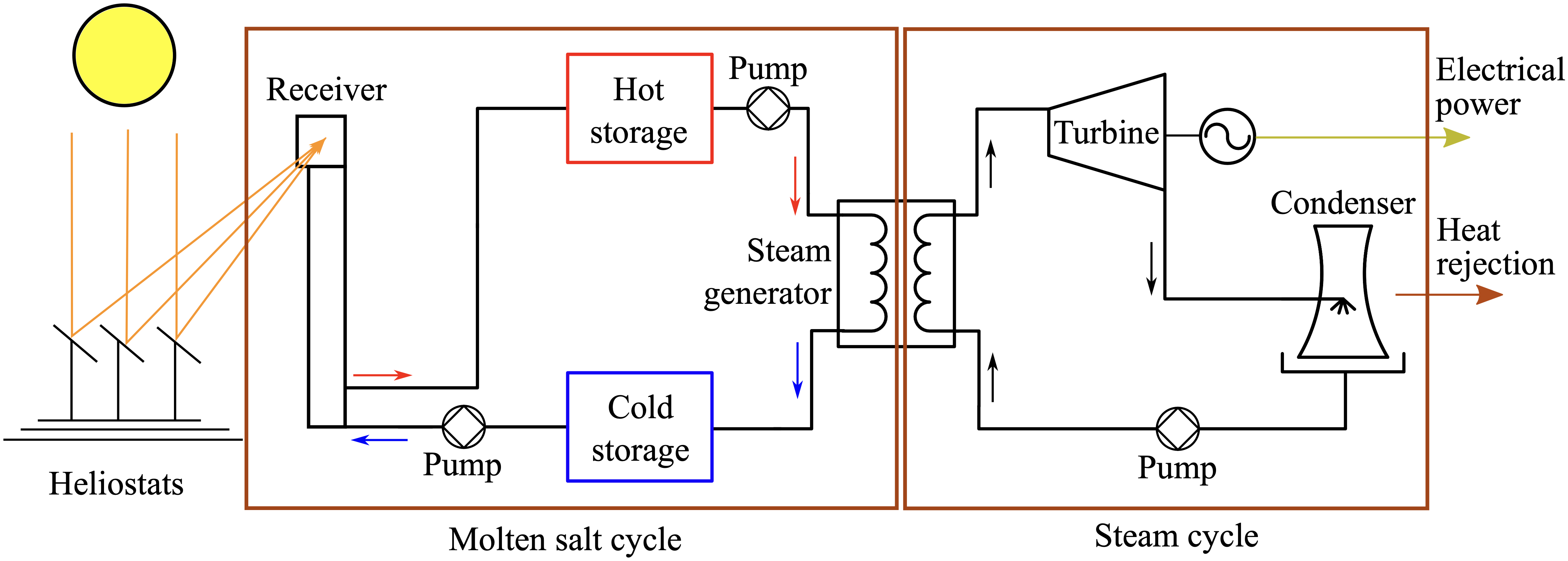
Figure 2: Cycle of the concentrated solar power (CSP) plant.

The heliostats field concentrates sunlight on the receiver, at the top of the tower. As the receiver heats up, thermal power is extracted by raising the temperature of a flow of molten salt pumped through its structure. The resulting hot molten salt is then directed to a hot storage tank until it is needed to drive the power block.

When electrical power is produced, hot molten salt is pumped though the steam generator to operate the power block. Heat is transferred to a flow of water on the other side of the steam generator which is transformed to superheated steam. Cold molten salt is recovered in the cold storage tank where it remains until it is pumped through the receiver again.

The power block is defined as a simple Rankine cycle with a single steam turbine. Superheated high-pressure steam drives a turbine coupled to an electrical generator. Low-pressure steam is then condensed and pumped back as liquid water though the steam generator.

2.4 Heliostats field

The optical subsystem consists of an array of heliostats (i.e., sun tracking mirrors) that reflect sunlight on the receiver. The design parameters used to define the heliostats field is given in Table 2. All of these parameters, except the latitude, are considered as optimization variables in Section 3.2.2.

Symbol	Quantity	Unit	Optim. var. in
			Tables 7 and 8
$\phi$	latitude	$\deg$	$-$
$W_{\mathrm{hf}}$	heliostats width	$\mathrm{m}$	$x_{2}$
$L_{\mathrm{hf}}$	heliostats length	$\mathrm{m}$	$x_{1}$
$H_{\mathrm{twr}}$	height of tower	$\mathrm{m}$	$x_{3}$
$N_{\mathrm{hf}}$	number of heliostats to fit in the field	$-$	$x_{6}$
$\theta_{\mathrm{hf}}$	angular width of the heliostats field	$\deg$	$x_{7}$
	on each side of the N-S axis
$R_{\mathrm{hf}}^{\min}$	minimum distance between heliostats	proportion of $H_{\mathrm{twr}}$	$x_{8}$
	and tower
$R_{\mathrm{hf}}^{\max}$	maximum distance between heliostats	proportion of $H_{\mathrm{twr}}$	$x_{9}$
	and tower
$H_{\mathrm{rcv}}$	receiver aperture height	$\mathrm{m}$	$x_{1}$, $x_{4}$
$W_{\mathrm{rcv}}$	receiver aperture width	$\mathrm{m}$	$x_{2}$, $x_{5}$

Table 2: List of design parameters for the heliostats field. The nomenclature of Table 1 is used. The latitude $\phi$ is a parameter fixed during optimization.

2.4.1 Generating the heliostats field

The heliostats are laid on a radially staggered grid that prevents blocking losses between them [57]. The grid is calculated as a function of individual heliostat dimensions ($W_{\mathrm{hf}}$ and $L_{\mathrm{hf}}$) and tower height ($H_{\mathrm{twr}}$). Figure 3 shows two examples of radially staggered grid layouts for identical heliostat dimensions but different tower heights.

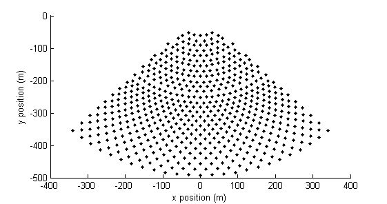
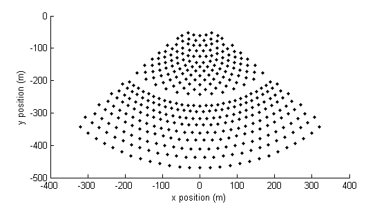
Figure 3: Examples of heliostats field layouts for tower heights of 120 $\mathrm{m}$ (left) and 70 $\mathrm{m}$ (right). The tower is located at (0,0).

2.4.2 Heliostats layout

Once the grid layout is determined, each position is rated according to the average optical efficiency $\eta$ that a potential heliostat would have on that location during the time window simulated. The optical efficiency of a heliostat is considered as the product of its cosine efficiency ($\eta_{\mathrm{cos}}$), the total atmospheric transmissivity from its position (constant $\tau$), and its spillage efficiency ( $\eta_{\mathrm{spl}}$). Both $\eta_{\mathrm{cos}}$ and $\eta_{\mathrm{spl}}$ depend on the orientation of each heliostat, which is itself dependent on the sun position. Both losses are approximated in [47] as a function of an analytical approximation of the Sun position [31]. Shadowing effects are not considered during this step, but are be accounted for when calculating the overall field’s performance. The instantaneous efficiency of a potential heliostat position is defined as:

$$\eta=\eta_{\mathrm{cos}}\eta_{\mathrm{spl}}\tau$$

The actual heliostats field is generated by occupying the first $N_{\mathrm{hf}}$ grid positions with the highest average optical efficiency for the given receiver aperture and tower height. For illustration, Figure 4 shows how the arrangement of 700 heliostats on the same spatial grid of 1,960 points varies with the receiver aperture width ($W_{\mathrm{rcv}}$). As the aperture narrows, the algorithm selects heliostats closer to the North-South axis to minimize spillage. For wider apertures, the selection is dictated by cosine efficiency and atmospheric attenuation.

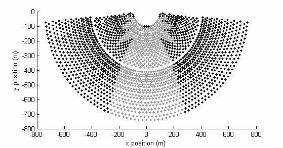
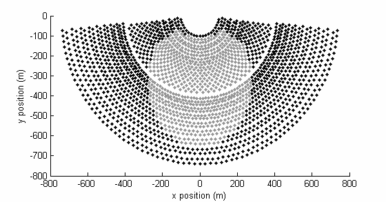
Figure 4: Examples of positions selected (in light gray) for receiver aperture widths of 3 $\mathrm{m}$ (left) and 15 $\mathrm{m}$ (right).

2.4.3 Sun radiation model

The power delivered to the receiver is estimated with a ray-tracing procedure corrected for spillage, attenuation and reflectivity losses. The sun is approximated as a distant point source so that rays are parallel to one another when they reach the field. Direct solar irradiance at the Earth’s surface is assumed to be 1 k$\mathrm{W}/\mathrm{m}^{2}$. Attenuation losses are calculated for a clear day [15]. Heliostats are modelled as flat surfaces with no aiming or tracking errors. Shading and cosine losses are inherently accounted for during ray-tracing. As a result of these simplifications, the predictions delivered by the model may overestimate the actual performance of the CSP plant.

2.5 The receiver

The receiver is modelled as a cavity with a rectangular aperture of sides $H_{\mathrm{rcv}}$ and $W_{\mathrm{rcv}}$. Molten salt is heated as it flows through an array of tubes laid on the inner surface of the cavity which are exposed to concentrated solar irradiation. Table 3 lists the design parameters used to model the receiver.

Symbol	Quantity	Unit	Optim. variables in
			Tables 7 and 8
$H_{\mathrm{rcv}}$	aperture height	$\mathrm{m}$	$x_{1}$, $x_{4}$
$W_{\mathrm{rcv}}$	aperture width	$\mathrm{m}$	$x_{2}$, $x_{5}$
$N_{\mathrm{rcv},\mathrm{tub}}$	number of tubes	$-$	$x_{4}$, $x_{7}$, $x_{10}$, $x_{11}$, $x_{16}$
$D_{\mathrm{rcv}}$	tubes outer diameter	$\mathrm{m}$	$x_{7}$, $x_{10}$, $x_{13}$, $x_{14}$, $x_{19}$
$d_{\mathrm{rcv}}$	tubes inner diameter	$\mathrm{m}$	$x_{6}$, $x_{9}$, $x_{12}$, $x_{13}$, $x_{18}$
$t_{\mathrm{rcv}}$	thickness of insulation	$\mathrm{m}$	$x_{5}$, $x_{8}$, $x_{11}$, $x_{12}$, $x_{17}$

Table 3: List of design parameters for the receiver unit. The nomenclature of Table 1 is used. $H_{\mathrm{rcv}}$ and $W_{\mathrm{rcv}}$ also appear in Table 2 since they impact the design of the heliostats field.

Heat lost back to the environment by reflection, re-radiation and conduction through the receiver wall is modelled with an iterative procedure described by Li et al. [48]. The absorbed heat rate is determined as the difference between the receiver thermal losses and the solar flux concentrated by the heliostats field on its aperture.

2.6 Thermal energy storage

The two thermal energy storage units, namely the cold tank and the hot tank, are large cylindrical stainless steel tanks where molten salt is kept until pumped to the power block or to the solar receiver. Both tanks have the same diameter and the cold storage height is 1.2 times larger than the hot storage height. Both tanks are protected by a layer of thermal insulation. Table 4 shows the list of design parameters that define the thermal storage component.

Symbol	Quantity	Unit	Optim. variables in
			Table 7
$t_{\mathrm{tank}}$	tanks insulation thickness	$\mathrm{m}$	$x_{4}$, $x_{5}$, $x_{13}$, $x_{14}$
$H_{\mathrm{tank}}$	height of the interior of the storage tanks	$\mathrm{m}$	$x_{2}$, $x_{11}$
$d_{\mathrm{tank}}$	diameter of the interior of the storage tanks	$\mathrm{m}$	$x_{3}$, $x_{12}$

Table 4: List of design parameters for the thermal storage units. The nomenclature of Table 1 is used. The subscript “$\mathrm{tank}$” can either be “$\mathrm{hot}$” or “$\mathrm{cold}$” and denotes whether the term refers to the hot or the cold tank e.g. $t_{cold}$ denotes the cold tank insulation thickness. The geometry of tanks is constrained by $d_{\mathrm{cold}}=d_{\mathrm{hot}}$ and $H_{\mathrm{cold}}=H_{\mathrm{hot}}\times 1.2$.

Thermal losses during storage are estimated as a function of the molten salt level and temperature with the heat loss model proposed by Zaversky et al. [62]. Figure 5 illustrates the heat transfer modes considered and defines the tanks design parameters. An identical insulation thickness for the wall and the ceiling surfaces is assumed. Natural convection and radiation patterns within the air and molten salt volumes are neglected. External radiation and forced convection losses to the atmosphere are considered assuming a constant wind speed of 6 $\mathrm{\mathrm{m}.s^{-1}}$ and normal atmospheric conditions. There are three channels of thermal losses from the molten salt when the tank is not at full capacity: conduction through the tank’s floor, conduction through the wet part of the cylindrical wall, and radiation from its top surface to the ceiling and the dry part of the cylindrical wall.

Figure 5: Thermal storage model parameters definition and loss processes. The nomenclature of Table 1 is used. The subscript “$\mathrm{tank}$” can either be “$\mathrm{hot}$” or “$\mathrm{cold}$”.

2.7 Heat exchanger (steam generator)

In general, commercial CSP plants obtain superheated steam from the combined action of a pre-heater, boiler and super-heater (e.g., [5]). None of these subsystems are explicitly modelled here. Instead, the steam generation unit is modelled only as a shell-and-tubes molten salt to water heat exchanger using the Effectiveness-NTU method [39], with the use of baffles that support the tubes, and the baffles cut corresponds to the portion of the shell inside diameter that is not covered by the baffle. Table 5 lists the design parameters associated with the heat exchanger.

Symbol	Quantity	Unit	Optim. variables
			in Table 8
$L_{\mathrm{sg}}$	length of tube passes	$\mathrm{m}$	$x_{12}$, $x_{21}$
$d_{\mathrm{sg}}$	inner diameter of tubes	$\mathrm{m}$	$x_{13}$, $x_{22}$
$D_{\mathrm{sg}}$	outer diameter of tubes	$\mathrm{m}$	$x_{14}$, $x_{23}$
$H_{\mathrm{sg},\mathrm{baf}}$	baffles cut	ratio of shell width	$x_{15}$, $x_{24}$
$N_{\mathrm{sg},\mathrm{baf}}$	number of baffles	$-$	$x_{16}$, $x_{25}$
$N_{\mathrm{sg},\mathrm{tub}}$	number of tubes	$-$	$x_{17}$, $x_{26}$
$N_{\mathrm{sg},\mathrm{sh},\mathrm{pass}}$	number of shell passes	$-$	$x_{18}$, $x_{27}$
$N_{\mathrm{sg},\mathrm{tub},\mathrm{pass}}$	number of tube passes per shell	$-$	$x_{19}$, $x_{28}$

Table 5: List of design parameters for the shell-and-tubes heat exchanger model. The nomenclature of Table 1 is used.

The heat exchanger model has two main functions. The first is to determine the flow of hot molten salt necessary to produce the required amount of pressurized steam for the turbine. For any simulation interval, the computed molten salt flow is dependent on the heat exchanger’s design parameters and the conditions of the hot storage. The second function is to compute the pressure drop and friction losses across the exchanger shells resulting from the molten salt flow. This is done using equations proposed by Gaddis and Gnielinsky [34]. Another way to model the heat exchange to produce superheated steam from molten salt is to suppose a perfect heat exchanger. Both approaches can be selected separately on different ${\sf solar}$ instances. In the idealized version, the heat exchanger has a 100% thermal efficiency without friction loss and the parameters describing its geometry are not required.

2.8 Molten salt cycle

Four subsystems are part of the molten salt cycle: the receiver, the two storage tanks, and the heat exchanger. The state and requirements of these subsystems depends on the state of other systems. For instance, the molten salt rate required by the heat exchanger to generate the necessary amount of steam at any moment depends not only on its own design parameters but also on the state of the hot storage: a higher inlet temperature will result in a smaller molten salt flow. Though because the rate of temperature drop of a storage unit is dependent on the stored mass, the two components are mutually dependent.

Similarly, the amount of molten salt that can be taken from the cold storage and heated to the design point conditions through the receiver is dependent on the temperature of the cold storage. Needless to say that the outlet conditions of both the receiver and the exchanger will too impact the storage units temperature and levels.

2.9 Power block

The only variable related to the power block is the choice of the turbine model. Technical data for a variety of commercial steam turbines used in CSP applications is retrieved from Siemens [58]. The dataset includes steam inlet pressures and temperatures required to operate each turbine, as well as their respective maximum and minimum power output. This part of the model is used to determine the amount of thermal power that ought to be extracted from the molten salt in order to meet the power demand.

Turbine efficiency is computed as a function of the inlet steam conditions and capacity usage ratio using a simple empirical model provided by Bahadori and Vuthaluru [14]. Steady-state conditions at all times are assumed, and turbine transients are neglected. A mechanical-to-electrical efficiency of 95% is assumed.

All components of the power cycle other than the turbine are idealized. The power required to pump the water condensate towards the heat exchanger is treated as part of the parasitic power consumption. No transient regime is considered and the whole cycle is assumed to shift instantly to match the demand profile. For most turbines, there exists a minimum value of power for which they can be operated. In the event that the demand is inferior to the minimum requirement for a turbine, the model will operate it at its minimum, least efficient regime, if possible, in order to reflect the fact that stopping the plant entirely in the middle of production is usually a bad operational option.

2.10 Auxiliary constraints models

Auxiliary models are used to provide constraints to the optimization problems. Without them, the solution to many of the problems would be trivial or impractical. For example, if the thickness of the insulation on the tanks is not counter-balanced by any other factor, it will always be set at its highest value. Similar reasoning applies for the heliostats: the best way to maximize the field’s surface efficiency is to fill it with a maximum number of very small heliostats that cover the entire field.

In order to provide a sufficient amount of constraints, four auxiliary models are used to estimate the equipment cost, parasitic loads, and the pressure both in the tubes of the receiver and heat exchanger.

2.10.1 Initial capital cost model

Although no complete life cycle cost analysis is integrated in the simulation, a simple initial investment cost model is provided in order to serve as a limiting factor for many of the design parameters. The data used to build the capital cost model was taken mostly from the National Renewable Energy Laboratory report on the SAM (System Advisor Model) [60] software and the Sandia Roadmap report [43]. The SAM model provides a means to determine the value of each component, but does so through an empirical model that mostly uses relations to the size or desired capacity of the plant. Its objective is to predict the potential cost of a project based on its sheer scale, rather than on specific technical characteristics. This turns out to be of little use as a limiting factor in optimization problems.

In order to link the cost of the components to their respective design parameters, relations have been established based on the price of materials. The total cost of the power plant is given below and is the sum of the costs of its subsystems, each one described as a function of some of the design parameters previously listed in their respective sections. These parameters also appear as the optimization variables of Tables 7 and 8.

$$\begin{split}\mbox{Total Cost}=\ &\underbrace{N_{\mathrm{hf}}C_{\mathrm{hf}}(L_{\mathrm{hf}},W_{\mathrm{hf}})}_{\text{Heliostats field}}+\underbrace{C_{\mathrm{twr}}(H_{\mathrm{twr}})}_{\text{ Tower}}+\underbrace{C_{\mathrm{rcv}}(H_{\mathrm{rcv}},W_{\mathrm{rcv}},t_{\mathrm{rcv}})}_{\text{Receiver}}+\\ &\underbrace{C_{\mathrm{hot}}(H_{\mathrm{hot}},d_{\mathrm{hot}},t_{\mathrm{hot}})}_{\text{ Hot storage}}+\underbrace{C_{\mathrm{cold}}(H_{\mathrm{cold}}=H_{\mathrm{hot}}\times 1.2,d_{\mathrm{cold}}=d_{\mathrm{hot}},t_{\mathrm{cold}})}_{\text{ Cold storage}}+\\ &\underbrace{C_{\mathrm{sg}}(S_{t},L_{\mathrm{sg}},d_{\mathrm{sg}},D_{\mathrm{sg}},H_{\mathrm{sg},\mathrm{baf}},N_{\mathrm{sg},\mathrm{baf}},N_{\mathrm{sg},\mathrm{tub}},N_{\mathrm{sg},\mathrm{sh},\mathrm{pass}},N_{\mathrm{sg},\mathrm{tub},\mathrm{pass}})}_{\text{ Steam generator}}+\\ &\underbrace{C_{\mathrm{trb}}(ST)}_{\text{ Turbine}}.\end{split}$$ (1)

2.10.2 Parasitic loads model

The parasitic load is the power required to operate the plant. The SAM considers a detailed set of parasitic load sources, including the heliostats electronic and mechanical control systems, piping anti-freeze protections, the molten salt pumps in the storage units, and the control systems of the receiver, heat exchanger and steam condenser. In the current work, components that are not directly necessary to describe the operation of a CSP plant (e.g., pump electronic controls) have been idealized. Since the pumps and pipes linking the main components of the system are not explicitly simulated or subject to optimization, their contribution to the losses is not considered. The evaluation of the parasitic load $P$ is thus comprised of five terms:

$$P=\underbrace{P_{\mathrm{rcv}}}_{\text{Receiver}}+\underbrace{P_{\mathrm{sg},\mathrm{sh}}}_{\begin{subarray}{c}\text{Steam}\\ \text{generator}\\ \text{ (shell)}\end{subarray}}+\underbrace{P_{\mathrm{sg},\mathrm{tub}}}_{\begin{subarray}{c}\text{Steam}\\ \text{generator}\\ \text{(tubes)}\end{subarray}}+\underbrace{P_{\mathrm{hf}}}_{\begin{subarray}{c}\text{Heliostats}\\ \text{field}\end{subarray}}+\underbrace{P_{\mathrm{hot}}+P_{\mathrm{cold}}}_{\begin{subarray}{c}\text{Storage}\\ \text{anti-freezing}\end{subarray}}.$$

The values of $P_{\mathrm{rcv}}$ and $P_{\mathrm{sg},\mathrm{tub}}$ are computed as the power required to pump a fluid through smooth tubes assuming a constant pump efficiency of 90%. For $P_{\mathrm{sg},\mathrm{sh}}$, a shell-side pressure drop model from [34] is used for shell-and-tubes heat exchangers. It is assumed that the pumps are capable of providing the required flow rate and pressure. The pressure differential is a function of both the flow rate and the geometry of the components. The term $P_{\mathrm{hf}}$ considers a constant and identical power consumption of 55 $\mathrm{W}$ per heliostat when operated (i.e., daytime) [6]. When the storage temperature drops below a certain threshold, the tanks are heated with $P_{\mathrm{hot}}+P_{\mathrm{cold}}$ to keep the temperature of both storage units above the molten salt’s melting point.

2.10.3 Maximum allowable pressure in tubes

The thickness and diameter of the tubes in both the receiver and steam generator is limited by the stress imposed on the steel by the internal fluid pressure. The stress is checked in each tube cross section so that it never exceeds the steel’s yield strength. For the sake of simplicity and time, creeping effects in metals are not considered. However, given that the system operates at high temperatures, this effect should be accounted for in more accurate models.

An exhaustive study of the heat exchanger system would also consider the stress imposed on the tubes by the molten salt flowing across them, thereby providing an additional limiting factor on the tubes length and spacing and the baffles spacing. In the present work, though, only the outward radial pressure exerted by the fluid flowing inside the tubes is considered.

3 A collection of optimization problem instances

The previous sections described the building blocks necessary to construct a collection of 10 optimization problem instances, provided by the ${\sf solar}$ code. This collection presents different variations of BBO benchmarks which can be used to test a wide range of algorithms. Each instance is uniquely characterised by its set of variables (Section 3.2.2), its objectives (Section 3.2.1), its constraints (Section 3.2.3) and its chosen fixed parameters, each of which is described in this section.

3.1 A general class of blackbox optimization problems

The instances of the collection belong to the following general minimization problem:

$$\min\limits_{\mathbf{x}\in{\mathbb{R}}^{n}}\ F(\mathbf{x})=\bigl{(}f_{1}(\mathbf{x}),f_{2}(\mathbf{x}),\ldots,f_{p}(\mathbf{x})\bigr{)}$$

subject to $$c_{i}(\mathbf{x})\leq 0 i\in\{1,2,\ldots,m\}$$ (2a)

subject to $$x_{j}\in{\mathbb{Z}} j\in{\cal J}$$ (2b)

subject to $$\ell\leq\mathbf{x}\leq u$$ (2c)

where $F:{\mathbb{R}}^{n}\rightarrow\overline{{\mathbb{R}}}^{p}$ is the objective function(s) to minimize, with $\overline{{\mathbb{R}}}:={\mathbb{R}}\cup\{\pm\infty\}$, subject to Constraints (2a), (2b), and (2c), and ${\cal J}\subseteq\{1,2,\ldots,n\}$ is the set of discrete variables. Constraint (2a) is compactly written as $C(\mathbf{x})\leq 0$ where $C(\mathbf{x})=\bigl{(}c_{1}(\mathbf{x}),c_{2}(\mathbf{x}),\ldots,c_{m}(\mathbf{x})\bigr{)}$ and with $C:{\mathbb{R}}^{n}\rightarrow\overline{{\mathbb{R}}}^{m}$. The vector $\mathbf{x}\in{\mathbb{R}}^{n}$ is the vector of optimization variables with bounds defined by (2c).

In practice, each component of $\mathbf{x}$ may be real, integer, binary or categorical. The indices of the integer and binary variables belong to the set ${\cal J}$. Categorical variables are also represented by integers.

While the underlying model is known and described in the previous section, the actual implementation is treated as a blackbox. For any value of the variable $\mathbf{x}$ and for any instance with $p$ objective functions and $m$ constraints, the computer simulation returns a formatted output in the form of a single vector $y$ containing the values of $F(\mathbf{x})$ and $C(\mathbf{x})$ such that

$$y(\mathbf{x})\ =\ \bigl{(}F(\mathbf{x}),C(\mathbf{x})\bigr{)}\ =\ \bigl{(}f_{1}(\mathbf{x}),f_{2}(\mathbf{x}),\ldots,f_{p}(\mathbf{x}),c_{1}(\mathbf{x}),c_{2}(\mathbf{x}),\ldots,c_{m}(\mathbf{x})\bigr{)}$$ (3)

The optimization process illustrated in Figure 6 consists in successively calling the blackbox with different values of $\mathbf{x}$, and using the corresponding output values $y(\mathbf{x})$ to dictate the next input values provided to the blackbox.

Figure 6: Blackbox optimization (BBO) process.

3.2 Ten blackbox instances

Ten instances, named ${\sf solar1.1}$ to ${\sf solar10.1}$, are implemented in a single C++ program that can be executed as a console application. The “.1” notation refers to the release 1.0 of the code, which is now frozen in time and guaranteed to never change. If bugs that may affect the outputs of the simulator are discovered, they will be fixed in another release (2.0 or more). This is the reason why users of ${\sf solar}$ are strongly encouraged to use the notation ${\sf solarX.1}$.

In order to compute $y(\mathbf{x})$, the following elements can be supplied to the ${\sf solar}$ code:

• the instance number (also called “problem ID” in the code) is an integer ranging from 1 to 10 that indicates which one of the 10 instances should be used;

• the input vector $\mathbf{x}$;

• the “seed” value, for the random seed of stochastic instances (see Section 4.4);

• the “rep” value, for the number of replications for the stochastic instances (see Section 4.4);

• the “fid” value, to select the fidelity of the output (see Section 4.6).

Only the instance number and the vector $\mathbf{x}$ are mandatory. The default values for the remaining elements correspond to deterministic instances with the best fidelity.

Each one of the 10 instances is characterized by a specific format for $\mathbf{x}$ (number of variables and their respective type and bounds) and $y$ (the objective function(s) and constraints), as summarized in Table 6.

Instance	# of variables			# of obj.	# of constraints			# of stoch. outputs	Multi
	cont.	discr. (cat.)	$n$	$p$	simu.	a priori (lin.)	$m$	(obj. or constr.)	fidelity
${\sf solar1.1}$	8	1 (0)	9	1	2	3 (2)	5	1	no
${\sf solar2.1}$	12	2 (0)	14	1	7	5 (3)	12	4	yes
${\sf solar3.1}$	17	3 (1)	20	1	8	5 (3)	13	5	yes
${\sf solar4.1}$	22	7 (1)	29	1	9	7 (5)	16	6	yes
${\sf solar5.1}$	14	6 (1)	20	1	8	4 (3)	12	0	no
${\sf solar6.1}$	5	0 (0)	5	1	6	0 (0)	6	0	no
${\sf solar7.1}$	6	1 (0)	7	1	4	2 (1)	6	3	yes
${\sf solar8.1}$	11	2 (0)	13	2	4	5 (3)	9	4	yes
${\sf solar9.1}$	22	7 (1)	29	2	10	7 (5)	17	6	yes
${\sf solar10.1}$	5	0 (0)	5	1	0	0 (0)	0	0	no

Table 6: Characteristics of the ten blackbox problem instances, including the number of continuous and discrete variables (including categorical), the number of objectives, the number of simulation and a priori constraints (see [46] and Section 4.3), and the number of stochastic outputs available through the -seed option (see Section 4.4). The last column indicates if the multifidelity feature is available through the -fid option (see Section 4.6). ${\sf solar10.1}$ is the unconstrained version based on ${\sf solar6.1}$. ${\sf solar2.1}$ is the only instance with a known analytical expression for the objective function.

3.2.1 Objectives and general description of each instance

This section gives a high-level description of each problem instance, and in particular, it describes the objective functions to optimize. When $p=1$, this is single-objective optimization problem, and when $p=2$, this is a biobjective optimization problem. The optimization is subject to various types of constraints that are described in Section 3.2.3.

${\sf solar1.1}$ - Maximize heliostats field energy output

This instance runs only the heliostats field model. It uses 9 variables of which one is discrete and the others are continuous. The objective is to maximize the energy collected by the receiver in 24 hours, while respecting a $50M budget and a maximum field area. The objective is subject to 5 relaxable and quantifiable constraints.

${\sf solar2.1}$ - Minimize the heliostats field surface (analytical objective)

This instance runs the whole power plant model and uses the idealized model for the heat exchanger. It uses 14 variables of which 2 are discrete and the others are continuous. The objective is $F(\mathbf{x})=f_{1}(\mathbf{x})={x_{3}^{2}(x_{9}^{2}-x_{8}^{2})x_{7}}\frac{\pi}{180}$ which corresponds to the heliostats field surface to minimize while satisfying the power demand peaking at 20 M$\mathrm{W}$ and respecting a $300M budget. The objective is subject to 14 relaxable and quantifiable constraints.

${\sf solar3.1}$ - Minimize total investment cost

This instance simulates the whole power plant and uses the idealized model for the steam generator. It uses 20 variables of which two are discrete, one is a categorical variable and 17 are continuous. The objective is to minimize the total investment cost while satisfying the demand and respecting a maximum field size. The simulation is done over 24 hours and the power plant is required to provide constant 10 M$\mathrm{W}$ during peak hours, between noon and 6 pm The objective is subject to 12 relaxable and quantifiable constraints.

${\sf solar4.1}$ - Minimize total investment cost

It is similar to ${\sf solar3.1}$, but with an increased level of complexity in the NTU-effectiveness steam generator model presented in Section 2.7. It uses 29 variables of which 6 are discrete, one is a categorical variable and 22 are continuous. The objective is to minimize the total investment cost while satisfying the demand and respecting a maximum field size. The simulation is done over 72 hours and the power plant is required to provide power at all time for a summer day demand profile peaking at 25 M$\mathrm{W}$. The objective is subject to 16 relaxable and quantifiable constraints.

${\sf solar5.1}$ - Maximize the satisfaction of the demand

This instance runs the molten salt loop and uses estimates of the performance of the heliostats field from a pre-computed database in order to reduce the computation time. It uses 20 variables of which 5 are discrete, one is a categorical variable and 14 are continuous. The power plant performance is simulated over a period of 30 days with an inconsistent field performance analogous to slightly unreliable weather conditions. The objective is to maximize the time for which the power plant is able to operate at nominal capacity. A surrogate model is available for this problem which consists in running the simulation on only a fraction of the 30 days and extrapolating the resulting performance over the 30 days. The objective is subject to 12 relaxable and quantifiable constraints.

${\sf solar6.1}$ - Minimize the cost of storage

This instance runs a predetermined power plant using the molten salt cycle and power block models. It uses 5 continuous variables. The objective is to minimize the cost of the thermal storage units so that the power plant is able to sustain a 100 M$\mathrm{W}$ electrical power output during 24 hours. Since the heliostats field is not being optimized, its hourly power output is read from a prerecorded file instead of being simulated, thus reducing the computation time. The objective is subject to 2 relaxable and quantifiable constraints and 4 unrelaxable and quantifiable constraints.

${\sf solar7.1}$ - Maximize receiver efficiency

This instance simulates the heliostats field and the receiver unit over a 24 hour period. It uses 7 variables, of which one is discrete and the others are continuous. The objective is to maximize the receiver efficiency. A surrogate version of the model can be used so that a much lower density of sunrays is used to evaluate the field’s performance. The objective is subject to 6 unrelaxable and quantifiable constraints.

${\sf solar8.1}$ - Maximize heliostats field performance and minimize cost (biobjective)

This instance runs the heliostats field and receiver models. It uses 13 variables, of which two are discrete and 11 are continuous. This is a biobjective problem of which the two objectives are to maximize the amount of energy transferred to the molten salt over a 24 hours period all while minimizing the total cost of the field, tower and receiver. The optimization is conducted over the design parameters of both the heliostats field and the receiver. The objectives are subject to 9 relaxable and quantifiable constraints.

${\sf solar9.1}$ - Maximize power and minimize losses (biobjective)

This instance simulates the entire power plant over a single day. It uses 29 variables, of which 6 are discrete, one is a categorical variable and 22 are continuous. This is a biobjective problem of which the two objectives are to maximize the generated electrical power and minimize the parasitic losses while respecting a $1.2B budget. The objectives are subject to 5 relaxable and quantifiable constraints and 12 unrelaxable and quantifiable constraints.

${\sf solar10.1}$ - Minimize the cost of storage (unconstrained)

This instance is the unconstrained version of ${\sf solar6.1}$ where the constraints are penalized in the objective with

$$F(\mathbf{x})=f_{1}(\mathbf{x})=\frac{h_{1}(\mathbf{x})}{10^{6}}+\frac{\left(g_{1}(\mathbf{x})^{2}+(2\times 10^{-6}g_{2}(\mathbf{x}))^{2}+g_{3}(\mathbf{x})^{2}+g_{4}(\mathbf{x})^{2}+g_{5}(\mathbf{x})^{2}+g_{6}(\mathbf{x})^{2}\right)}{2}$$

with $h_{1}$ the objective function of ${\sf solar6.1}$ and $g_{i}$ the violation of Constraint $i$ of ${\sf solar6.1}$ with $i\in\{1,2,\ldots,6\}$. These weights have been fixed empirically.

Category	Symbol	Quantity	Unit	Type	Lower	Upper	Instances	Optim.
					bound	bound		variable
Heliostats field	$L_{\mathrm{hf}}$	Heliostats length	$\mathrm{m}$	cont.	1	40	1 2 3 4 8 9	$x_{1}$
	$W_{\mathrm{hf}}$	Heliostats width	$\mathrm{m}$	cont.	1	40	1 2 3 4 8 9	$x_{2}$
	$H_{\mathrm{twr}}$	Tower height	$\mathrm{m}$	cont.	20	250	1 2 3 4 8 9	$x_{3}$
	$H_{\mathrm{rcv}}$	Receiver aperture height	$\mathrm{m}$	cont.	1	30	1 2 3 4 8 9	$x_{4}$
							7	$x_{1}$
	$W_{\mathrm{rcv}}$	Receiver aperture width	$\mathrm{m}$	cont.	1	30	1 2 3 4 8 9	$x_{5}$
							7	$x_{2}$
	$N_{\mathrm{hf}}$	Number of heliostats to fit	$-$	discr.	1	$+\infty$	1 2 3 4 8 9	$x_{6}$
	$\theta_{\mathrm{hf}}$	Field angular width	$\deg$	cont.	1	89	1 2 3 4 8 9	$x_{7}$
	$R_{\mathrm{hf}}^{\min}$	Min. distance from tower	ratio	cont.	0	20	1 2 3 4 8 9	$x_{8}$
	$R_{\mathrm{hf}}^{\max}$	Max. distance from tower	ratio	cont.	1	20	1 2 3 4 8 9	$x_{9}$
	$T_{\mathrm{rcv}}^{out}$	Receiver outlet temp.	$\mathrm{K}$	cont.	793	995	2 3 4 9	$x_{10}$
							5 6 10	$x_{1}$
							7	$x_{3}$
	$H_{\mathrm{hot}}$	Hot storage height	$\mathrm{m}$	cont.	1	50	3 4 9	$x_{11}$
					1	30	5	$x_{2}$
					2	50	6 10	$x_{2}$
	$d_{\mathrm{hot}}$	Hot storage diameter	$\mathrm{m}$	cont.	1	30	3 4 9	$x_{12}$
					1	30	5	$x_{3}$
					2	30	6 10	$x_{3}$
	$t_{\mathrm{hot}}$	Hot storage insulation thickness	$\mathrm{m}$	cont.	0.01	5	3 4 9	$x_{13}$
					0.01	2	5	$x_{4}$
					0.01	5	6 10	$x_{4}$
Heat transfer loop	$t_{\mathrm{cold}}$	Cold storage insulation thickness	$\mathrm{m}$	cont.	0.01	5	3 4 9	$x_{14}$
					0.01	2	5	$x_{5}$
					0.01	5	6 10	$x_{5}$
	$T_{\mathrm{cold}}^{\min}$	Min. cold storage temp.	$\mathrm{K}$	cont.	495	650	3 4 9	$x_{15}$
							5	$x_{6}$
	$N_{\mathrm{rcv},\mathrm{tub}}$	Receiver number of tubes	$-$	discr.	1	9,424	2	$x_{11}$
						9,424	3	$x_{16}$
						7,853	4 9	$x_{16}$
						1,884	5	$x_{7}$
						8,567	7	$x_{4}$
						7,853	8	$x_{10}$
	$t_{\mathrm{rcv}}$	Receiver insulation thickness	$\mathrm{m}$	cont.	0.01	5	2	$x_{12}$
					0.01	5	3 4 9	$x_{17}$
					0.10	2	5	$x_{8}$
					0.01	5	7	$x_{5}$
(continued in Table 8)					0.01	5	8	$x_{11}$

Table 7: The 29 possible optimization variables (1/2). The “$\times H_{\mathrm{twr}}$” unit means that the distances from tower ($x_{8}$ and $x_{9}$) are expressed as multiples of $H_{\mathrm{twr}}$.

3.2.2 Optimization variables

The optimization variables of Problem (2c) are $\mathbf{x}\in{\mathbb{R}}^{n}$. While all the variables are by definition continuous, Equation (2b) imposes that $x_{j}\in{\mathbb{Z}}$ for $j\in{\cal J}$. In addition, the type of turbine ($ST$) is a categorical variable with 8 possible values. Tables 7 and 8 list all possible 29 variables, their characteristics and bounds ($\ell\leq\mathbf{x}\leq u$ (2c)), depending in the instance. Only Instances ${\sf solar4.1}$ and ${\sf solar9.1}$ include all of them as optimization variables. Some optimization variables have no upper bounds. As some algorithms require all bounds to be defined, this task is left to the user that can create a reasonable upper bound from the suggested lower bounds and initial values. The simulation parameters and the values of the instance-specific constraints are chosen to reflect realistic engineering problems. For instance, budgets, maximum field surface, and power output requirements are derived from known data on existing similar power plants. The exact numerical values to which these numerous parameters are set in each problem instance can be found in [47].

Category	Symbol	Quantity	Unit	Type	Lower	Upper	Instances	Optim.
					bound	bound		variable
	$d_{\mathrm{rcv}}$	Receiver tubes inner diameter	$\mathrm{m}$	cont.	0.005	0.1	2	$x_{13}$
							3 4 9	$x_{18}$
							5	$x_{9}$
							7	$x_{6}$
Heat transfer loop							8	$x_{12}$
(continued from Table 7)	$D_{\mathrm{rcv}}$	Receiver tubes outer diameter	$\mathrm{m}$	cont.	0.0050	0.1	2	$x_{14}$
					0.0050	0.1	3	$x_{19}$
					0.0060	0.1	4 9	$x_{19}$
					0.0050	0.1	5	$x_{10}$
					0.0055	0.1	7	$x_{7}$
					0.0060	0.1	8	$x_{13}$
Steam generator	$S_{t}$	Tubes spacing	$\mathrm{m}$	cont.	0.007	0.2	4 9	$x_{20}$
					0.006	0.2	5	$x_{11}$
	$L_{\mathrm{sg}}$	Tubes length	$\mathrm{m}$	cont.	0.5	10	4 9	$x_{21}$
							5	$x_{12}$
	$d_{\mathrm{sg}}$	Tubes inner diameter	$\mathrm{m}$	cont.	0.005	0.1	4 9	$x_{22}$
							5	$x_{13}$
	$D_{\mathrm{sg}}$	Tubes outer diameter	$\mathrm{m}$	cont.	0.006	0.1	4 9	$x_{23}$
							5	$x_{14}$
	$H_{\mathrm{sg},\mathrm{baf}}$	Baffles cut	ratio	cont.	0.15	0.4	4 9	$x_{24}$
							5	$x_{15}$
(exchanger)	$N_{\mathrm{sg},\mathrm{baf}}$	Number of baffles	$-$	discr.	2	$+\infty$	4 9	$x_{25}$
							5	$x_{16}$
	$N_{\mathrm{sg},\mathrm{tub}}$	Number of tubes	$-$	discr.	1	$+\infty$	4 9	$x_{26}$
							5	$x_{17}$
	$N_{\mathrm{sg},\mathrm{sh},\mathrm{pass}}$	Number of shell passes	$-$	discr.	1	10	4 9	$x_{27}$
							5	$x_{18}$
	$N_{\mathrm{sg},\mathrm{tub},\mathrm{pass}}$	Number of tube passes	$-$	discr.	1	9	4 9	$x_{28}$
							5	$x_{19}$
Powerblock	$ST$	Type of turbine	$-$	discr.	1	8	3 5	$x_{20}$
				(cat.)			4 9	$x_{29}$

Table 8: The 29 possible optimization variables (2/2).

3.2.3 Constraints

The taxonomy of constraints of [46] allows to better describe the different types of constraints in Problem (2c). Constraints (2a) and (2c) (bounds) are quantifiable: the inequality format ensures that $c_{i}(\mathbf{x})$ ($i\in\{1,2,\ldots,m\}$) or $\mathbf{x}$ measure the distance to feasibility or infeasibility. On the contrary, Constraints (2b) (discrete nature of some variables) are nonquantifiable. Constraints (2b) and (2c) (discrete variables and bounds) are also a priori constraints: they can be evaluated without executing the ${\sf solar}$ simulator. Depending on the instances, some of the constraints of (2a) are also a priori (including linear constraints), while the others are of the type simulation (the execution of the ${\sf solar}$ simulator is necessary to evaluate them). A priori constraints are also considered to be unrelaxable: They represent known relations between some variables and need to always be respected for the simulator to be executed: for example, the inner diameter of a tube must be smaller than its outer diameter. The simulation constraints, on the contrary, are relaxable, meaning that their potential violation does not prevent to execute the simulation. Hence, they can be violated during an optimization process, which can be very useful, as long as the final proposed solution is feasible. Finally, there are hidden constraints consisting mostly of code glitches or instability; some solutions may cause the code to crash or otherwise malfunction. These constraints are not given explicitly in the problem definition as they are unknown. Section 4.3 provides more details on how ${\sf solar}$ manages a priori and hidden constraints.

The ${\sf solar}$ code, for a given $\mathbf{x}$, returns $y(\mathbf{x})$ as defined in (3), which, for the constraints, corresponds to the left hand-sides $c_{i}(\mathbf{x})$ of Constraints (2a), for $i\in\{1,2,\ldots,m\}$. Constraints (2b) and (2c) must be considered by the optimization method, and if they are not satisfied, the ${\sf solar}$ simulator will not execute. The bounds and the discrete variables are visible in Tables 7 and 8. Hence the following of this section focuses on how Constraints (2a) are defined in ${\sf solar1.1}$ to ${\sf solar9.1}$ (${\sf solar10.1}$ is unconstrained). The number and type of these constraints are given in Table 6.

The a priori constraints are given below, using the $\mathbf{x}$ vector. However, since $\mathbf{x}$ is not defined the same for each instance, it is necessary to consult Tables 7 and 8.

Linear a priori constraints:

Constraints details are shown in Table 9.

	${\sf solar1.1}$	${\sf solar2.1}$	${\sf solar3.1}$	${\sf solar4.1}$	${\sf solar5.1}$	${\sf solar6.1}$	${\sf solar7.1}$	${\sf solar8.1}$	${\sf solar9.1}$
Constraint	Tower is at least twice as high as heliostats
Indexation	$c_{3}$	$c_{4}$	$c_{3}$	$c_{3}$	$-$	$-$	$-$	$c_{2}$	$c_{4}$
Equation	$2x_{1}\leq x_{3}$
Constraint	Minimum distance from tower is lower than the maximum distance from tower
Indexation	$c_{4}$	$c_{5}$	$c_{4}$	$c_{4}$	$-$	$-$	$-$	$c_{3}$	$c_{5}$
Equation	$x_{8}\leq x_{9}$
Constraint	Receiver tubes inside diameter is lower than the outside diameter
Indexation	$-$	$c_{11}$	$c_{10}$	$c_{10}$	$c_{6}$	$-$	$c_{3}$	$c_{6}$	$c_{11}$
Equation	$x_{i}\leq x_{j}$
$i$, $j$	$-$	13, 14	18, 19	18, 19	9, 10	$-$	6, 7	12, 13	18, 19
Constraint	Tubes outer diameter is between the tubes inside diameter and the tubes spacing
Indexation	$-$	$-$	$-$	$c_{14},c_{15}$	$c_{10},c_{11}$	$-$	$-$	$-$	$c_{16},c_{17}$
Equation	$x_{i}\leq x_{j}\leq x_{k}$
$i$, $j$, $k$	$-$	$-$	$-$	22, 23, 20	13, 14, 11	$-$	$-$	$-$	22, 23, 20

Table 9: Linear a priori constraints in Instances ${\sf solar1.1}$ to ${\sf solar9.1}$ (${\sf solar10.1}$ is unconstrained). A “$-$” means the constraint is not part of the instance.

Nonlinear a priori constraints:

Constraints details are shown in Table 10. In ${\sf solar2.1}$, the left hand side of the heliostats field surface area constraint corresponds to the objective function to minimize (see Section 3.2.1).

	${\sf solar1.1}$	${\sf solar2.1}$	${\sf solar3.1}$	${\sf solar4.1}$	${\sf solar5.1}$	${\sf solar6.1}$	${\sf solar7.1}$	${\sf solar8.1}$	${\sf solar9.1}$
Constraint	Heliostats field surface area is lower than the maximum field surface area
Indexation	$c_{2}$	$c_{1}$	$c_{1}$	$c_{1}$	$-$	$-$	$-$	$c_{1}$	$c_{3}$
Equation	$\pi x_{3}^{2}(x_{9}^{2}-x_{8}^{2})x_{7}/180\leq a$
$a$ [hectares]	195	400	80	200	$-$	$-$	$-$	400	500
Constraint	Number of tubes in receiver fits inside receiver
Indexation	$-$	$c_{12}$	$c_{11}$	$c_{11}$	$c_{7}$	$-$	$c_{5}$	$c_{7}$	$c_{12}$
Equation	$x_{i}x_{j}\leq a\frac{\pi}{2}$
$i$, $j$, $a$	$-$	11, 14, $x_{5}$	16, 19, $x_{5}$	16, 19, $x_{5}$	7, 10, 6	$-$	4, 7, $x_{2}$	10, 13, $x_{5}$	16,19,$x_{5}$

Table 10: Nonlinear a priori constraints in Instances ${\sf solar1.1}$ to ${\sf solar9.1}$ (${\sf solar10.1}$ is unconstrained). A “$-$” means the constraint is not part of the instance.

Simulation constraints:

These constraints depend on some outputs of the simulation, described below. Lengths, distances, tower size, tubes spacing and diameters are all in meters, energy and parasitic load are expressed in k$\mathrm{W}$h, costs are in $, surfaces in hectares, temperatures in Kelvin, and pressures in $\mathrm{MPa}$. The constraints are relaxable and quantifiable (code QRSK in [46]). Moreover, some of these constraints correspond to stochastic outputs of the program. This behavior is controlled with the -seed option (see Section 4.4). Constraints details are shown in Table 11.

	${\sf solar1.1}$	${\sf solar2.1}$	${\sf solar3.1}$	${\sf solar4.1}$	${\sf solar5.1}$	${\sf solar6.1}$	${\sf solar7.1}$	${\sf solar8.1}$	${\sf solar9.1}$
Constraint	The required number of heliostats ($x_{6}$) can fit in the heliostats field
Indexation	$c_{5}$	$c_{6}$	$c_{5}$	$c_{5}$	$-$	$-$	$-$	$c_{4}$	$c_{6}$
Constraint	The cost of plant is lower than the budget
Indexation	$c_{1}$	$c_{3}$	$-$	$-$	$c_{1}$	$-$	$c_{1}$	$-$	$c_{1}$
Budget limit	$50M	$300M	$-$	$-$	$100M	$-$	$45M	$-$	$1.2B
Constraint	Compliance to demand
Indexation	$-$	$c_{2}$	$c_{2}$	$c_{2}$	$-$	$c_{1}$	$-$	$-$	$-$
Stochastic	$-$	yes	yes	yes	$-$	no	$-$	$-$	$-$
Constraint	Minimal acceptable energy production
Indexation	$-$	$-$	$-$	$-$	$-$	$-$	$-$	$c_{8}$	$c_{2}$
Stochastic	$-$	$-$	$-$	$-$	$-$	$-$	$-$	yes	yes
Constraint	Parasitic losses are lower than a ratio of the generated output
Indexation	$-$	$-$	$-$	$c_{13}$	$c_{9}$	$-$	$c_{6}$	$c_{9}$	$c_{14}$
Limit ratio	$-$	$-$	$-$	18%	18%	$-$	3%	8%	20%
Stochastic	$-$	$-$	$-$	yes	no	$-$	yes	yes	yes
Constraint	Storage is back at least at its original conditions
Indexation	$-$	$-$	$c_{13}$	$-$	$-$	$c_{6}$	$-$	$-$	$-$
Stochastic	$-$	$-$	yes	$-$	$-$	no	$-$	$-$	$-$
Constraint	Molten salt temperature does not fall below the melting point in hot storage
Indexation	$-$	$c_{8}$	$c_{7}$	$c_{7}$	$c_{3}$	$c_{3}$	$-$	$-$	$c_{8}$
Stochastic	$-$	yes	yes	yes	no	no	$-$	$-$	yes
Constraint	Molten salt temperature does not fall below the melting point in cold storage
Indexation	$-$	$c_{9}$	$c_{8}$	$c_{8}$	$c_{4}$	$c_{4}$	$-$	$-$	$c_{9}$
Stochastic	$-$	yes	yes	yes	no	no	$-$	$-$	yes
Constraint	Molten salt temperature does not fall below the melting point in steam generator outlet
Indexation	$-$	$-$	$c_{9}$	$c_{9}$	$c_{5}$	$-$	$-$	$-$	$c_{10}$
Stochastic	$-$	$-$	no	yes	no	$-$	$-$	$-$	yes
Constraint	Receiver outlet temperature is greater than the steam turbine inlet temperature
Indexation	$-$	$c_{12}$	$c_{12}$	$c_{12}$	$c_{8}$	$c_{5}$	$-$	$-$	$c_{13}$
Constraint	Pressure in receiver tubes is lower than yield pressure
Indexation	$-$	$c_{7}$	$c_{6}$	$c_{6}$	$c_{2}$	$c_{2}$	$c_{2}$	$c_{5}$	$c_{7}$
Stochastic	$-$	yes	yes	yes	no	no	yes	yes	yes
Constraint	Pressure in steam generator tubes is lower than yield pressure
Indexation	$-$	$-$	$-$	$c_{16}$	$c_{12}$	$-$	$-$	$-$	$c_{17}$

Table 11: Nonlinear a priori constraints in Instances ${\sf solar1.1}$ to ${\sf solar9.1}$ (${\sf solar10.1}$ is unconstrained). A “$-$” means the constraint is not part of the instance. When stochasticity is not specified, constraints are deterministic.

4 The ${\sf solar}$ package for benchmarking

This section describes the ${\sf solar}$ package version 1.0. The correct way to refer to a specific instance requires the version number of the package. For example, tests involving the third instance with the version 1.x of ${\sf solar}$ should be denoted by ${\sf solar3.1}$: the first number is the instance, and the second is the main number of the version.

The complexity and nature of the ${\sf solar}$ BBO problems depend on the selected instances and the options passed to the ${\sf solar}$ framework. The number and nature of variables, the number of constraints and objectives have already been mentioned. In addition, for testing the agility of optimization methods to handle BBO problems, some features on the outputs can be present or not in ${\sf solar}$ instances. These features are discussed in the following sections as such: variables types in Section 4.2, constraint types and failure to return valid outputs in Section 4.3, stochasticity in Section 4.4, static surrogate models in Section 4.5, multifidelity in Section 4.6.

Figure 7 illustrates the inner working of the ${\sf solar}$ framework. For a given $\mathbf{x}$, the first step consists in verifying if the a priori constraints are satisfied as detailed in Section 4.3. Then, the simulator is possibly called many times, with different random seeds using the prescribed fidelity. In this case, the output interpreter returns averaged values of $F$ and of $C$ in the vector $y$. In addition, the input file can contain several vectors $\mathbf{x}$ and the output interpreter returns several vectors $y$.

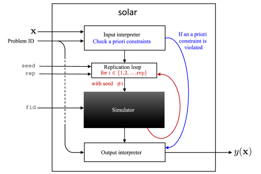
Figure 7: The ${\sf solar}$ framework. “Problem ID” is the instance number between 1 and 10.

4.1 Software utilization

The README file from the GitHub package provides the necessary instructions to build ${\sf solar}$ from source. As the software has been developed for comparable benchmarking, an in-house random number generator is used to guarantee that outputs are platform and compiler independent when calling the executable with the same settings. For this reason it is strongly encouraged to verify this behaviour by running the command  solar -check before conducting any benchmarking. Once the ${\sf solar}$ version is stated to be valid, all performance results can be compared to any studies which used the same ${\sf solar}$ version for benchmarking.

Basic utilization information can be obtained from the executable by running the command  solar -h. This describes how to run a simulation as well as the available options for stochasticity and fidelity and their default parameters; further information on these modes is given in their respective subsections. In addition, the best known values for single-objective instances (one replication, full fidelity, default random seed of zero) are reported.

Details on Instance id are obtained with the command solar -h id. Table 12 summarizes the information displayed by the command for all instances. The command also shows the suggested bounds on variables and a suggested starting point (feasible or infeasible) given in the NOMAD parameters syntax. Additional information about the simulation can be obtained in verbose mode by adding -v to the command. When the provided point satisfies all a priori and hidden constraints, all the outputs are successfully computed by the simulator. In this case, the flag cnt_eval=true (“count evaluation”). This flag is displayed only in verbose mode.

The ${\sf solar}$ executable is obtained by building all the source code files. A more direct access to the ${\sf solar}$ evaluator on a given instance is also possible (see the source code in the main_minimal or main_minimal_2 functions in main.cpp). The flag cnt_eval is an output of the evaluator call function eval_x.

4.2 Mixed integer, categorical and unbound variables

It is quite common for synthetic blackbox instances to have only real and bounded input variables. This however is only the case for Instances ${\sf solar6.1}$ and ${\sf solar10.1}$. Every other instance contains one or more integer inputs, as detailed in Tables 7 and 8. If a non-integer value is provided in the input file for an integer variable, all the outputs returned by the code will be $10^{20}$. Filtering or rounding values of input variables should be performed before launching ${\sf solar.}$

Furthermore, Instances ${\sf solar3.1}$, ${\sf solar4.1}$, ${\sf solar5.1}$, and ${\sf solar9.1}$ also contain categorical inputs. Whilst these take their values from a discrete set, they do not possess any ordering properties [8]. A framework for modeling such variables in the context of BBO is presented in [9].

As an added difficulty, at least one integer input is always unbound, meaning approaches such as Latin hypercube Sampling which requires an upper and lower bound for every input variable cannot be directly applied and need to be adapted in some way. Note that as described in Section 4.1, calling the help command for a particular instance provides, among others, a suggested starting point for optimization. The suggested starting value for unbound input variables can be used as a guide for what input range to explore, although it provides no guarantees in terms of proximity to an optimal point.

Instance	A priori	Simulated deterministic	Simulated stochastic
${\sf solar1.1}$	$c_{2},c_{3},c_{4}$	$c_{1},c_{5}$	$f_{1}$
${\sf solar2.1}$	$f_{1},c_{1},c_{4},c_{5},c_{10},c_{11}$	$c_{3},c_{6},c_{12}$	$c_{2},c_{7},c_{8},c_{9}$
${\sf solar3.1}$	$c_{1},c_{3},c_{4},c_{10},c_{11}$	$f_{1},c_{5},c_{9},c_{12}$	$c_{2},c_{6},c_{7},c_{8},c_{13}$
${\sf solar4.1}$	$c_{1},c_{3},c_{4},c_{10},c_{11},c_{14},c_{15}$	$f_{1},c_{5},c_{12},c_{16}$	$c_{2},c_{6},c_{7},c_{8},c_{9},c_{13}$
${\sf solar5.1}$	$c_{6},c_{7},c_{10},c_{11}$	$f_{1},c_{1},c_{2},c_{3},c_{4},c_{5},c_{8},c_{9},c_{12}$
${\sf solar6.1}$		$f_{1},c_{1},c_{2},c_{3},c_{4},c_{5},c_{6}$
${\sf solar7.1}$	$c_{3},c_{5}$	$c_{1},c_{4}$	$f_{1},c_{2},c_{6}$
${\sf solar8.1}$	$c_{1},c_{2},c_{3},c_{6},c_{7}$	$f_{2},c_{4}$	$f_{1},c_{5},c_{8},c_{9}$
${\sf solar9.1}$	$c_{3},c_{4},c_{5},c_{11},c_{12},c_{15},c_{16}$	$c_{1},c_{6},c_{13},c_{17}$	$f_{1},f_{2},c_{2},c_{7},c_{8},c_{9},c_{10},c_{14}$
${\sf solar10.1}$		$f_{1}$

Table 12: Classification of the outputs of the ten blackbox instances as either a priori, simulated and deterministic or simulated and stochastic.

4.3 Constraints evaluation

The ${\sf solar}$ package includes a priori (QUAK) [46] constraints with given expressions (see Section 3.2.3). The specific outputs are shown in Table 12. They are fast to evaluate compared to simulation constraints. Hence, the simulator does not start if at least one is violated. In this case, the values for the a priori constraints are returned but those for the remaining simulation constraints are set to $10^{20}$. This evaluation should not be counted during an optimization, as indicated by the raised flag cnt_eval=false (available only in verbose mode or when calling directly the ${\sf solar}$ evaluator). Table 13 gives an estimation of how frequently different types of constraints are violated for each instance.

Instance	Eval. (nb)	LH sampling (10,000 points)			NOMAD 3
	$=400n$	feas. AP (%)	feas. (%)	hidden (%)	feas. AP (%)	feas. (%)	hidden (%)
${\sf solar1.1}$	3,600	29.0	4.28	0	96.9	73.0	0.417
${\sf solar2.1}$	5,600	17.9	0	0	91.8	6.89	0
${\sf solar3.1}$	8,000	8.63	0	0	94.9	11.4	0.100
${\sf solar4.1}$	11,600	0.112	0	0	84.8	28.0	0.0603
${\sf solar5.1}$	3,000	1.60	0.10	0	88.2	14.3	0
${\sf solar6.1}$	2,000	90.1	4.95	0	100	40.0	0.557
${\sf solar7.1}$	2,800	46.4	14.2	0	82.7	50.9	0.143
${\sf solar8.1}$	5,200	0.942	0	0	80.2	60.3	0.135
${\sf solar9.1}$	11,600	0.845	0	0.0948	64.6	9.82	0.793
${\sf solar10.1}$	2,000	100	100	0	100	100	0

Table 13: Percentage of feasibility of a priori constraints (“feas. AP”), of all constraints (“feas.”) and of hidden constraints (“hidden”) for Latin hypercube sampling and for NOMAD 3 [45]. For comparability between instances, an evaluation budget of 400 times the instance dimension is given to each instance. The NOMAD optimization of ${\sf solar6.1}$ converged and stopped after 1,976 evaluations, and 150$n$ evaluations are given to ${\sf solar5.1}$ because its evaluation time is high.

Hidden (NUSH) [46] constraints are present in some instances. Some bugs may still be present in the code, as is often the case in real blackbox problems. Moreover, some a priori constraints may not be explicitly given. For example, when $x_{3}x_{8}\neq 0$ is not verified in ${\sf solar1.1}$, a hidden constraint is violated. Some hidden constraints can even stop an evaluation before any simulation is launched (see Figure 7), causing the flag cnt_eval=false to be raised. When a hidden constraint is violated, the ${\sf solar}$ evaluation does not complete, and some simulated outputs return the value $10^{20}$. Not all outputs are necessarily affected by a violated hidden constraint. Note that for most cases, the closer to 1 the fidelity is, the less likely it is to violate a hidden constraint. This is not always the case, as for ${\sf solar3.1}$, it is possible to find a point such that a hidden constraint is violated only with fidelity 1. To benchmark a blackbox with hidden constraints, the authors recommend ${\sf solar3.1}$ with lower fidelities. This way, violating a hidden constraint is still relatively rare. To benchmark in a situation of highly occurring hidden constraints violation, the authors recommend the STYRENE problem [7].

4.4 Stochasticity

Table 12 shows that seven of the ten instances contain at least one stochastic output. The collection of instances of this type provides a variety of benchmarks for algorithm development with different characteristics. Specifically, ${\sf solar1.1}$ provides a classical stochastic optimization benchmark where only the objective function is stochastic, but some deterministic constraints also exist. Instance ${\sf solar7.1}$ contains a stochastic objective function as well as some stochastic constraints. Instances ${\sf solar2.1}$, ${\sf solar3.1}$ and ${\sf solar4.1}$, on the other hand, provide less traditional benchmarks where the objective function is deterministic, but some of the constraints are stochastic. Finally, for an added layer of benchmark complexity, Instances ${\sf solar8.1}$ and ${\sf solar9.1}$ are defined with two objectives and stochastic outputs.

4.4.1 The seed argument (random seed)

For reproducibility purposes, every stochastic behaviour stems from a seed, controlled with the -seed argument passed to the ${\sf solar}$ command. The custom pseudo-random number generator used by ${\sf solar}$ also guarantees stochastic reproducibility for the same inputs and specified seed. This behaviour is verified when running the command solar -check after compiling ${\sf solar.}$ The default seed value is 0, and thus no stochastic behaviour will be observed between executions if this parameter is not specifically modified. To enable stochasticity, set -seed=diff to randomly generate a different seed each time, leading to non-reproducible behaviour. Users can also choose to seed the random generator with a chosen integer s with the argument -seed=s. Note that another potential use of fixing the seed is the creation of different deterministic instances of the same simulation. Figure 8 shows how stochasticity leads to different levels of variability for the stochastic outputs of all instances. Even within the same instance, variability can be very different among the outputs; in ${\sf solar9.1}$ for example Constraints 7, 8 and 10 exhibit little variations compared to Constraint 2. Choosing how to approach different stochastic levels for each of the outputs simultaneously is up to the technique being assessed.

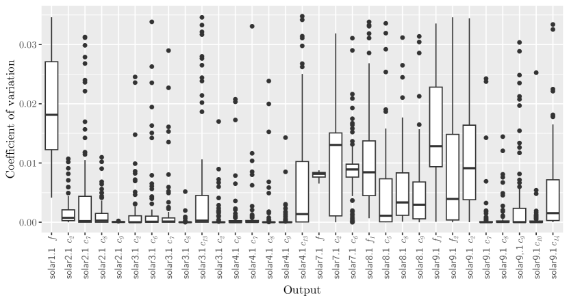
Figure 8: Distribution of the coefficient of variation of the stochastic outputs of all instances. Each box plot shows the coefficient of variation calculated at 100 randomly selected points, calculated for 100 seeds each. Each box plot shows the median (thick black line), the interquartile range (rectangle), and the min and max range (vertical lines) excluding outliers (black points). Note that a few outliers outside of the plot range are not shown here for clarity.

4.4.2 The rep argument (replications)

A common algorithmic approach to handle stochastic outputs involves repeatedly sampling the same location and taking the output average. In order to aid practitioners in the use of ${\sf solar}$, this approach can be directly queried from the simulator via the argument -rep=r with ${\tt r}\in{\mathbb{N}}^{+}$ passed to the ${\sf solar}$ command. Passing this parameter will run the specified simulation a total of r times and return only the average of the outputs. The default -rep value is 1. Additionally, when the number of repetitions is greater than one, the -seed argument is now used to generate different repetitions. This means that running a ${\sf solar}$ instance with -seed=s and -rep=r will always result in the same repetitions, the same output values. Again, this is true across all platforms and compilers.

Alternatively, another algorithmic approach is to repeatedly sample a point until a stopping rule is satisfied. The Gauss-distribution criteria, described in [17], has been implemented. In practice, it is activated by choosing ${\tt r}$ as a real in $(0,1)$ for the -rep=r argument. In this mode, ${\tt r}$ represents the probability that all the stochastic outputs are stabilized within 3 significant digits. A replication number limit of $5\times 10^{4}$ ensures the existence of an upper bound on computational time. Table 14 shows that closer to an optimum, the number of replications needed to reach each probability is generally considerably higher, although exceptions are present. Notice that even with probabilities as low as $0.05$, it is possible to reach the replication limit. Finally one must be careful when using this parameter within a time budget. Notice that ${\sf solar2.1}$ at the best known point with probability $0.5$ took almost 12 days to reach $5\times 10^{4}$ replications.

Instance	Input	nb of replications for multiple r values					CPU time (seconds) for multiple r values
		0.05	0.25	0.5	0.75	0.95	0.05	0.25	0.5	0.75	0.95
${\sf solar1.1}$	$\mathbf{x}^{0}$	7	125	558	1,558	4,299	0	9	58	275	1,567
	$\mathbf{x}^{\star}$	10	36	94	232	678	84	324	825	2,076	5,824
${\sf solar2.1}$	$\mathbf{x}^{0}$	15	164	688	2,033	5,837	136	1,497	6,480	19,574	58,875
	$\mathbf{x}^{\star}$	884	22,571	50k	50k	50k	14,059	468,595	1,017k	1,018k	1,004k
${\sf solar3.1}$	$\mathbf{x}^{0}$	7	29	194	562	1,582	12	50	324	1,025	2,996
	$\mathbf{x}^{\star}$	13,153	50k	50k	50k	50k	38,904	147,781	142,858	$-$	$-$
${\sf solar4.1}$	$\mathbf{x}^{0}$	7	7	7	7	7	13	13	13	13	13
	$\mathbf{x}^{\star}$	3,723	50k	50k	50k	50k	13,578	266,764	$-$	$-$	242,440
${\sf solar7.1}$	$\mathbf{x}^{0}$	7	16	60	148	369	25	57	212	525	1,311
	$\mathbf{x}^{\star}$	50k	50k	50k	50k	50k	256,757	$-$	$-$	$-$	$-$
${\sf solar8.1}$	$\mathbf{x}^{0}$	7	7	38	122	415	43	43	232	789	2,560
	$\mathbf{x}^{a}$	7	7	12	18	65	49	49	87	128	450
${\sf solar9.1}$	$\mathbf{x}^{0}$	26	285	1,164	3,366	9,591	70	774	3,237	9,960	33,161
	$\mathbf{x}^{b}$	8	85	486	1,344	3,681	31	369	2,054	6,407	21,180

Table 14: Number of replications and CPU time (with an Apple M2 max) for some instances when using five different values of -rep=r in $(0,1)$. Input $\mathbf{x}^{\star}$ denotes the best known point at the time of writing, whereas $\mathbf{x}^{0}$ denotes the starting point suggested for the problem, far from $\mathbf{x}^{\star}$ (these points are further described in Table 15). For multiobjective instances, since no known point dominates all the others, random points $\mathbf{x}^{a}$ and $\mathbf{x}^{b}$ are shown. For a probability parameter higher than another where the replication number limit was reached at the same point, the simulation is sometimes not run since it would surely reach the limit as well, and a “$-$” is shown.

4.5 Surrogate models

In the present context of Problem (2c), a surrogate is a simplified version of the functions $F$ and $C$ that are replaced by approximations which are less computationally expensive. These surrogates are constructed by relaxing some internal parameters within the simulation. For example, a surrogate may trace fewer rays, or sample the performance of the plant at fewer instants over the time window than the real blackbox.

Some solvers take advantage of such alternative models to conduct the optimization, and use the original model only to verify promising solutions found with the surrogate. The surrogate management framework [22] proposes ways to exploit surrogates in optimization problems.

A surrogate model used by an optimization algorithm can be dynamic, meaning the algorithm builds its own model and adjusts it during the optimization, or static, meaning it is given to the algorithm beforehand. With the ${\sf solar}$ package, there are different ways to create static surrogate models. First, by lowering the fidelity, a wide range of static surrogates with variable precision are created. Second, by considering a chosen number of replications for a stochastic blackbox to be the truth, any lower number of replications results in a static surrogate. A static surrogate model can also be achieved by lowering both the fidelity and the number of replications.

4.6 Multifidelity

With Instances ${\sf solar2.1}$, ${\sf solar3.1}$, ${\sf solar4.1}$, ${\sf solar7.1}$, ${\sf solar8.1}$, ${\sf solar9.1}$, and ${\sf solar10.1}$, a fidelity argument -fid=$\phi$ can be passed to the ${\sf solar}$ command, with $\phi\in[0,1]$. The default $\phi$ value is 1. Lowering the fidelity generally leads to faster computational times, at the cost of degraded accuracy of the simulation results. As ${\sf solar}$ is a simulation engine, both the time and accuracy reduction do not follow a specific formula. With -fid=0, only the a priori outputs are evaluated, while the others are set to $10^{20}$. Figure 9 shows the relationship between fidelity and execution time on the single-objective multifidelity instances.

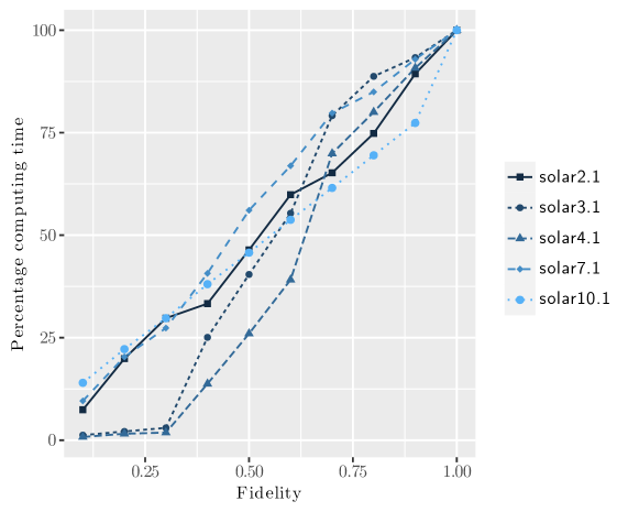
Figure 9: Computation time for different fidelities on Instances ${\sf solar2.1}$, ${\sf solar3.1}$, ${\sf solar4.1}$, ${\sf solar7.1}$, and ${\sf solar10.1}$, with respect to a fidelity of 1.

To focus on simulation time, only points that satisfy all a priori constraints are considered. As it can be seen, the percentage reduction in time is roughly linear with the reduction in fidelity for all instances.

In all constrained instances where the fidelity parameter is available, a number of constraints are affected by the -fid parameter. This is a unique feature among BBO benchmarking problems, despite the fact that many industrial BBO problems have this property [3]. Trivially, a set of bi-fidelity benchmarks similar to [59] can easily be generated by selecting pairs of fidelities.

Figure 10 shows how lowering the fidelity can lead to the incorrect labeling of whether a constraint is violated or not. Certain constraints such as constraint 6 for ${\sf solar7.1}$ are not much impacted, whereas others such as constraint 13 for ${\sf solar4.1}$ is only reliable for a fidelity of 0.9 or higher.

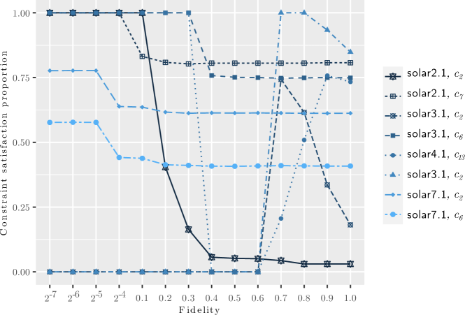
Figure 10: Proportion of points within a small radius of the best known feasible solutions which satisfy particular constraints at different fidelities.

Figure 11 showcases on ${\sf solar10.1}$ the impact fidelity has both on computational time and percentage error compared to using a fidelity of 1. Instance ${\sf solar10.1}$ is an unconstrained problem, for which modifying the fidelity impacts only the objective function. As the figure shows, whilst providing no guarantees, increasing the fidelity leads to a consistent increase in time as evidenced by points of the same fidelity lying on the same height. At the same time, an increase in fidelity leads to a consistent decrease in error, as evidenced by a reduction in the width in which points of higher fidelities lie. Interestingly, the vast majority of points feature an underestimation of the objective value.

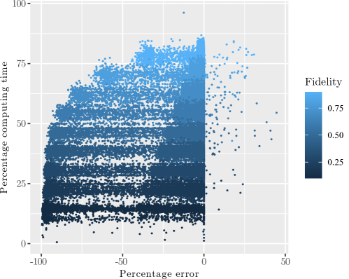
Figure 11: Computational time and error on ${\sf solar10.1}$ objective value on sampled points using different fidelities. Each sampled point is associated with a colored dot on the plot at coordinate $(x,y)$. The $y$-value denotes the percentage time taken compared to running the same sample point with fidelity of 1, and the $x$-value denotes the error relative to the objective function value of the same sample point with fidelity of 1. Note that a negative error denotes an underestimation, and positive error a overestimation of the objective function.

4.7 Examples of optimization results

Part of the challenge of building a new blackbox for BBO benchmarking is making sure that the resulting optimization problems meet some basic requirements: they need to have non-trivial optimal solutions, and they need to be acceptably functional. For instance, if a problem would be to minimize the cost of the designed power plant, it has to contain constraints sufficient to ensure that an optimization algorithm would not cling to a trivial solution such as a power plant with no heliostats at all that has a very low cost but also produces absolutely no energy.

The best known points, at the time of writing, for the single-objective instances, are noted $\mathbf{x}^{\star}$ and have been collected in the recent years with the help of several beta-testers (they are named in the acknowledgments). Along with the suggested starting points, noted $\mathbf{x}^{0}$, they are summarized in Table 15. The best known values $f_{1}(\mathbf{x}^{\star})$ are also indicated in the GitHub repository, but not the coordinates $\mathbf{x}^{\star}$ themselves.

In all cases, the best known solutions are non-trivial, as noticeable by the low number of active bounds at $\mathbf{x}^{\star}$ and the number of saturated inequality constraints. Other constraints closed to saturation are not reported in the table but this may be an indication that the objective values may be further reduced although probably not easily. Moreover, in Instances ${\sf solar1.1}$, ${\sf solar3.1}$ and ${\sf solar7.1}$, the objective value at $\mathbf{x}^{\star}$ has been significantly reduced compared with $f_{1}(\mathbf{x}^{0})$.

	${\sf solar1.1}$	${\sf solar2.1}$	${\sf solar3.1}$	${\sf solar4.1}$	${\sf solar5.1}$	${\sf solar6.1}$	${\sf solar7.1}$	${\sf solar10.1}$
$f_{1}(\mathbf{x}^{0})$	-122,506	753,527	107,541,652	78,622,308	-30.0615	4,136,232	-2,768	1,880
$f_{1}(\mathbf{x}^{\star}$)	-902,504	841,840	70,813,885	108,197,236	-28.8817	43,954,935	-4,973	42
viol. constr. at $\mathbf{x}^{0}$	feasible	$c_{2}$, $c_{6}$, $c_{7}$	$c_{2}$	$c_{2}$, $c_{5}$	$c_{2}$, $c_{5}$, $c_{9}$	$c_{1}$, $c_{6}$	$c_{2}$, $c_{6}$	feasible
active constr. at $\mathbf{x}^{0}$	$c_{5}$	$-$	$c_{5}$	$-$	$c_{4}$	$-$	$-$	$-$
active bounds at $\mathbf{x}^{0}$	$-$	$u_{7}$	$-$	$u_{21}$, $\ell_{27}$	$\ell_{16}$, $\ell_{20}$	$-$	$-$	$-$
active constr. at $\mathbf{x}^{\star}$	$c_{5}$	$c_{2}$, $c_{6}$	$c_{2}$, $c_{5}$, $c_{8}$	$c_{2}$, $c_{5}$	$-$	$c_{1}$	$c_{4}$	$-$
active bounds at $\mathbf{x}^{\star}$	$-$	$-$	$\ell_{14}$	$u_{15}$	$u_{6}$, $\ell_{16}$, $\ell_{19}$	$u_{1}$, $u_{3}$, $\ell_{5}$	-	$\ell_{5}$

Table 15: Comparison of the values of the initial points ($\mathbf{x}^{0}$) with the values of the best known points ($\mathbf{x}^{\star}$), for the single-objective instances. These values are rounded, and when negative, they correspond to a maximization problem. The lines “viol. constr.”, “active constr.”, and “active bounds” indicate which constraints or bounds are active or violated, for $\mathbf{x}^{0}$ or $\mathbf{x}^{\star}$.

Data profiles obtained on ${\sf solar6.1}$ with 30 different starting points generated by Latin Hypercube sampling show that the optimization solvers tested (NOMAD 3 [45], NOMAD 4 [12] and CMA-ES [37]) do not systematically produce the best known solution.

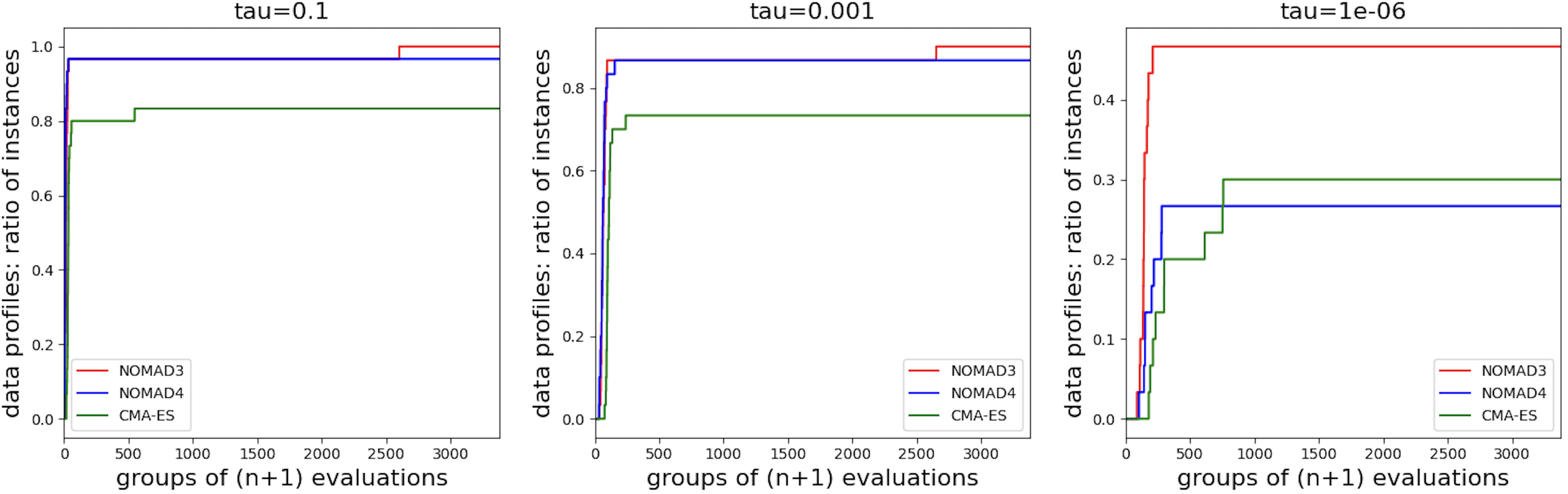
Figure 12: Data profiles obtained on ${\sf solar6.1}$ using 30 different starting points generated by Latin Hypercube sampling with the NOMAD 3 [45], NOMAD 4 [12] and CMA-ES [37] solvers.

As shown in Table 12, ${\sf solar}$ provides two multiobjective instances for benchmarking, namely ${\sf solar8.1}$ and ${\sf solar9.1}$. Figure 13 displays examples of non-dominated solutions of both instances when using the default seed, fidelity and replication inputs. These plots give an indication of the characteristics of the respective Pareto fronts. The non-dominated solutions obtained by different solvers are distinct, suggesting that ${\sf solar8.1}$ and ${\sf solar9.1}$ are not trivial problems.

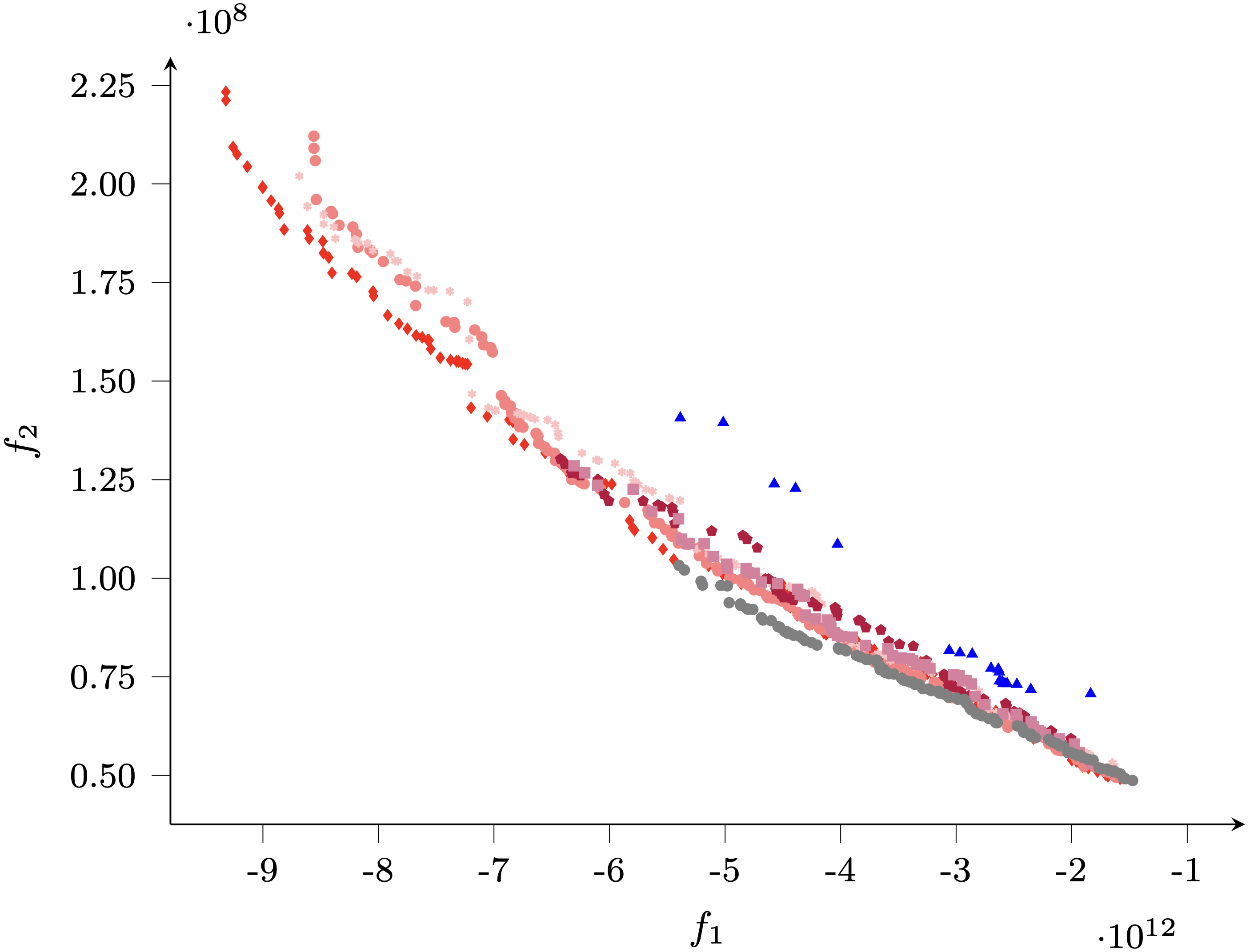
Figure 13: Examples of non-dominated solutions for ${\sf solar8.1}$ obtained during multiobjective optimizations conducted in [19] using various solvers and a maximal budget of 5,000 evaluations.

4.8 Sensitivity of optimization solutions

The best solutions obtained during the preliminary tests shown previously often feature saturated or close to saturation inequality constraints. Navigating the design space in a region around best solution presents algorithmic and numerical challenges for most solvers. The sensitivity of constraints feasibility around such points can be a good indicator of the difficulty of the task.

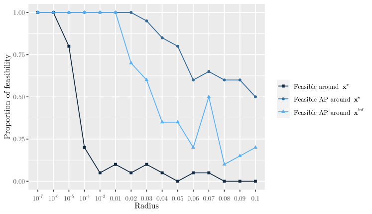
Figure 14: Plot showing how the feasibility of ${\sf solar4.1}$ points is sensitive to small changes. For different radii $r$, “Feasible around $\mathbf{x}^{\star}$” shows the proportion of feasible points sampled in $B_{r}(\mathbf{x}^{\star})$, “Feasible AP around $\mathbf{x}^{\star}$” shows the proportion of points sampled in $B_{r}(\mathbf{x}^{\star})$ that satisfy all a priori constraints, and “Feasible AP around $\mathbf{x}^{inf}$” shows the proportion of points sampled in $B_{r}(\mathbf{x}^{inf})$ that satisfy all a priori constraints. Here, $\mathbf{x}^{\star}$ is the best known solution for ${\sf solar4.1}$ at the time of writing and $\mathbf{x}^{inf}$ is an infeasible point.

Figure 14 shows the proportion of feasible points (all constraints or only a priori constraints) around two types of points obtained with ${\sf solar4.1}$. When considering all constraints, it can be noted that achieving feasibility requires to be very close to $\mathbf{x}^{\star}$.

In a realistic optimization problem, the direction and amplitude of change in objective function value play a role in a solver progress. If objective function reduction is possible close to current best solution maybe there is room for improvement while still maintaining saturated inequality constraints. When solver stops, for an optimization solver end user, this can be an incentive to relax saturated inequality constraints (if possible) to obtain more gain. Figure 15 shows the sensitivity of the objective function of ${\sf solar10.1}$ near $\mathbf{x}^{\star}$. Hence, we believe that ${\sf solar10.1}$ is non trivial with characteristics similar to what is found in real life optimization problems and represents a good challenge for solvers.

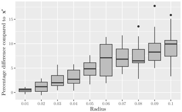
Figure 15: Percentage change in the objective function of ${\sf solar10.1}$ at different distances from a best known solution $\mathbf{x}^{\star}$.

5 Discussion

There are very few industrial or real-life publicly available BBO problems. This works addresses this issue by introducing ${\sf solar,}$ a collection of benchmark problem instances for BBO. ${\sf solar}$ contains ten instances of a blackbox that simulates a concentrated solar power plant. The instances differ in terms of variables, constraints, stochasticity and number of objective functions. ${\sf solar}$ is coded in standard C++ and is publicly available as a stand-alone open source package on GitHub. Practitioners and algorithm developers are encouraged to test their methods with this blackbox and to participate by sending their best optimization logs and results to nomad@gerad.ca in order to update the database of results on the ${\sf solar}$ GitHub page. Future work includes the definition and release of new instances of the blackbox to the community.

References

- [1] A. Abhat. Low temperature latent heat thermal energy storage: Heat storage materials. Solar Energy, 30(4):313--332, 1983.
- [2] M.A. Abramson. Mixed Variable Optimization of a Load-Bearing Thermal Insulation System Using a Filter Pattern Search Algorithm. Optimization and Engineering, 5(2):157--177, 2004.
- [3] S. Alarie, C. Audet, M. Diago, S. Le Digabel, and X. Lebeuf. Hierarchically constrained multi-fidelity blackbox optimization. Technical Report G-2023-66, Les cahiers du GERAD, 2023.
- [4] S. Alarie, C. Audet, A.E. Gheribi, M. Kokkolaras, and S. Le Digabel. Two decades of blackbox optimization applications. EURO Journal on Computational Optimization, 9:100011, 2021.
- [5] A. Alobaidli, B. Sanz, K. Behnke, T. Witt, D. Viereck, and M.-A. Schwarz. Shams 1 - Design and operational experiences of the 100MW - 540∘C CSP plant in Abu Dhabi. AIP Conference Proceedings, 1850(1):020001, 2017.
- [6] C.A. Amadei, G. Allesina, P. Tartarini, and W. Yuting. Simulation of GEMASOLAR-based solar tower plants for the Chinese energy market: influence of plant downsizing and Location change. Renewable energy, 55:366--373, 2013.
- [7] C. Audet, V. Béchard, and S. Le Digabel. Nonsmooth optimization through Mesh Adaptive Direct Search and Variable Neighborhood Search. Journal of Global Optimization, 41(2):299--318, 2008.
- [8] C. Audet and J.E. Dennis, Jr. Pattern Search Algorithms for Mixed Variable Programming. SIAM Journal on Optimization, 11(3):573--594, 2001.
- [9] C. Audet, E. Hallé-Hannan, and S. Le Digabel. A General Mathematical Framework for Constrained Mixed-variable Blackbox Optimization Problems with Meta and Categorical Variables. Operations Research Forum, 4(12), 2023.
- [10] C. Audet and W. Hare. Derivative-Free and Blackbox Optimization. Springer Series in Operations Research and Financial Engineering. Springer, Cham, Switzerland, 2017.
- [11] C. Audet and M. Kokkolaras. Blackbox and derivative-free optimization: theory, algorithms and applications. Optimization and Engineering, 17(1):1--2, 2016.
- [12] C. Audet, S. Le Digabel, V. Rochon Montplaisir, and C. Tribes. Algorithm 1027: NOMAD version 4: Nonlinear optimization with the MADS algorithm. ACM Transactions on Mathematical Software, 48(3):35:1--35:22, 2022.
- [13] C. Audet, G. Savard, and W. Zghal. Multiobjective Optimization Through a Series of Single-Objective Formulations. SIAM Journal on Optimization, 19(1):188--210, 2008.
- [14] A. Bahadori and H.B. Vuthaluru. Estimation of performance of steam turbines using a simple predictive tool. Applied Thermal Engineering, 30(13):1832--1838, 2010.
- [15] J. Ballestrín and A. Marzo. Solar radiation attenuation in solar tower plants. Solar Energy, 86(1):388--392, 2012.
- [16] V. Beiranvand, W. Hare, and Y. Lucet. Best practices for comparing optimization algorithms. Optimization and Engineering, 18(4):815--848, 2017.
- [17] M. Bicher, M. Wastian, D. Brunmeir, and N. Popper. Review on Monte Carlo Simulation Stopping Rules: How Many Samples Are Really Enough? Simulation Notes Europe, 32(1):1--8, 2022.
- [18] J. Bigeon, S. Le Digabel, and L. Salomon. DMulti-MADS: Mesh adaptive direct multisearch for bound-constrained blackbox multiobjective optimization. Computational Optimization and Applications, 79(2):301--338, 2021.
- [19] J. Bigeon, S. Le Digabel, and L. Salomon. Handling of constraints in multiobjective blackbox optimization. Technical Report G-2022-10, Les cahiers du GERAD, 2022. To appear in Computational Optimization and Applications.
- [20] A.J. Booker, J.E. Dennis, Jr., P.D. Frank, D.W. Moore, and D.B. Serafini. Managing surrogate objectives to optimize a helicopter rotor design -- further experiments. AIAA Paper 1998--4717, Presented at the 8th AIAA/ISSMO Symposium on Multidisciplinary Analysis and Optimization, St. Louis, 1998.
- [21] A.J. Booker, J.E. Dennis, Jr., P.D. Frank, D.B. Serafini, and V. Torczon. Optimization using surrogate objectives on a helicopter test example. In J. Borggaard, J. Burns, E. Cliff, and S. Schreck, editors, Optimal Design and Control, Progress in Systems and Control Theory, pages 49--58, Cambridge, Massachusetts, 1998. Birkhäuser.
- [22] A.J. Booker, J.E. Dennis, Jr., P.D. Frank, D.B. Serafini, V. Torczon, and M.W. Trosset. A Rigorous Framework for Optimization of Expensive Functions by Surrogates. Structural and Multidisciplinary Optimization, 17(1):1--13, 1999.
- [23] J.I. Burgaleta, S. Arias, and D. Ramirez. Gemasolar, the first tower thermosolar commercial plant with molten salt storage. In Proceedings of the SolarPACES 2011 conference on concentrating solar power and chemical energy systems, Granada, Spain, 2011.
- [24] T.D. Choi and C.T. Kelley. Superlinear convergence and implicit filtering. SIAM Journal on Optimization, 10(4):1149--1162, 2000.
- [25] J. Cox, W.T. Hamilton, A.M. Newman, and J. Martinek. Optimal sizing and dispatch of solar power with storage. Optimization and Engineering, 24(4):2579--2617, 2023.
- [26] J. Craig. Bluebird developer manual, 2002. Available at http://www.civil.uwaterloo.ca/jrcraig/pdf/bluebird_developers_manual.pdf.
- [27] A.L Custódio, M. Emmerich, and J.F.A Madeira. Recent Developments in Derivative-Free Multiobjective Optimization. Computational Technology Reviews, 5(1):1--30, 2012.
- [28] A.L. Custódio, K. Scheinberg, and L.N. Vicente. Methodologies and software for derivative-free optimization. In T. Terlaky, M.F. Anjos, and S. Ahmed, editors, Advances and Trends in Optimization with Engineering Applications, MOS-SIAM Book Series on Optimization, chapter 37. SIAM, Philadelphia, 2017.
- [29] E.D. Dolan and J.J. Moré. Benchmarking optimization software with performance profiles. Mathematical Programming, 91(2):201--213, 2002.
- [30] L.P. Drouot and M.J. Hillairet. The Themis program and the 2500-KW Themis solar power station at Targasonne. Journal of Solar Energy Engineering, 106(1):83--89, 1984.
- [31] J.A. Duffie and W.A. Beckman. Solar engineering of thermal processes. John Wiley and Sons, 2013.
- [32] M.M. Farid, A.M. Khudhair, S.A.K. Razack, and S. Al-Hallaj. A review on phase change energy storage: materials and applications. Energy Conversion and Management, 45(9):1597--1615, 2004.
- [33] K.R. Fowler, J.P. Reese, C.E. Kees, J.E. Dennis Jr., C.T. Kelley, C.T. Miller, C. Audet, A.J. Booker, G. Couture, R.W. Darwin, M.W. Farthing, D.E. Finkel, J.M. Gablonsky, G. Gray, and T.G. Kolda. Comparison of derivative-free optimization methods for groundwater supply and hydraulic capture community problems. Advances in Water Resources, 31(5):743--757, 2008.
- [34] E.S. Gaddis and V. Gnielinski. Pressure drop on the shell side of shell-and-tube heat exchangers with segmental baffles. Chemical Engineering and Processing: Process Intensification, 36(2):149--159, 1997.
- [35] A.E. Gheribi, A.D. Pelton, and J.-P. Harvey. Determination of optimal compositions and properties for phase change materials in a solar electric generating station. Solar Energy Materials and Solar Cells, 210:110506, 2020.
- [36] N. Hansen, A. Auger, R. Ros, O. Mersmann, T. Tušar, and D. Brockhoff. COCO: a platform for comparing continuous optimizers in a black-box setting. Optimization Methods and Software, 36(1):114--144, 2021.
- [37] N. Hansen and A. Ostermeier. Completely derandomized self-adaptation in evolution strategies. Evolutionary Computation, 9(2):159--195, 2001.
- [38] W. Hock and K. Schittkowski. Test Examples for Nonlinear Programming Codes, volume 187 of Lecture Notes in Economics and Mathematical Systems. Springer, Berlin, Germany, 1981.
- [39] F.P. Incropera, D.P. DeWitt, T.L. Bergman, and A.S. Lavine. Fundamentals of heat and mass transfer 6th edition, 2006.
- [40] M. Kenisarin and K. Mahkamov. Solar energy storage using phase change materials. Renewable and Sustainable Energy Reviews, 11(9):1913--1965, 2007.
- [41] M.M. Kenisarin. High-temperature phase change materials for thermal energy storage. Renewable and Sustainable Energy Reviews, 14(3):955--970, 2010.
- [42] M. Kokkolaras, C. Audet, and J.E. Dennis, Jr. Mixed variable optimization of the Number and composition of heat intercepts in a thermal insulation system. Optimization and Engineering, 2(1):5--29, 2001.
- [43] G.J Kolb, C.K. Ho, T.R. Mancini, and J.A. Gary. Power Tower Technology Roadmap and Cost Reduction Plan. Technical Report SAND2011-2419, Sandia National Laboratories, 2011.
- [44] J. Larson, M. Menickelly, and S.M. Wild. Derivative-free optimization methods. Acta Numerica, 28:287--404, 2019.
- [45] S. Le Digabel. Algorithm 909: NOMAD: Nonlinear Optimization with the MADS algorithm. ACM Transactions on Mathematical Software, 37(4):44:1--44:15, 2011.
- [46] S. Le Digabel and S.M. Wild. A taxonomy of constraints in black-box simulation-based optimization. Optimization and Engineering, 25(2):1125--1143, 2024.
- [47] M. Lemyre Garneau. Modelling of a solar thermal power plant for benchmarking blackbox optimization solvers. Master’s thesis, Polytechnique Montréal, 2015. Available at https://publications.polymtl.ca/1996/.
- [48] X. Li, W. Kong, Z. Wang, C. Chang, and F. Bai. Thermal model and thermodynamic performance of molten salt cavity receiver. Renewable Energy, 35(5):981--988, 2010.
- [49] Y. Luo, Z. Wang, J. Zhu, T. Lu, G. Xiao, F. Chu, and R. Wang. Multi-objective robust optimization of a solar power tower plant under uncertainty. Energy, 238:121716, 2022.
- [50] A. Manno, E. Amaldi, F. Casella, and E. Martelli. A local search method for costly black-box problems and its application to CSP plant start-up optimization refinement. Optimization and Engineering, 21(4):1563--1598, 2020.
- [51] L.S. Matott, K. Leung, and J. Sim. Application of MATLAB and Python optimizers to two case studies involving groundwater flow and contaminant transport modeling. Computers and Geosciences, 37(11):1894--1899, 2011.
- [52] J.J. Moré and S.M. Wild. Benchmarking Derivative-Free Optimization Algorithms. SIAM Journal on Optimization, 20(1):172--191, 2009.
- [53] N. Ploskas and N.V. Sahinidis. Review and comparison of algorithms and software for mixed-integer derivative-free optimization. Journal of Global Optimization, 82(3):433--462, 2022.
- [54] L.M. Rios and N.V. Sahinidis. Derivative-free optimization: a review of algorithms and comparison of software implementations. Journal of Global Optimization, 56(3):1247--1293, 2013.
- [55] H.H. Rosenbrock. An automatic method for finding the greatest or least value of a function. The Computer Journal, 3(3):175--184, 1960.
- [56] A. Sharma, V.V. Tyagi, C.R. Chen, and D. Buddhi. Review on thermal energy storage with phase change materials and applications. Renewable and Sustainable Energy Reviews, 13(2):318--345, 2009.
- [57] F.M.F Siala and M.E Elayeb. Mathematical formulation of a graphical method for a no-blocking heliostat field layout. Renewable Energy, 23(1):77--92, 2001.
- [58] Siemens. Steam turbines for CSP plants. https://www.siemens-energy.com/global/en/home/products-services/solutions-industry/renewable-energy/concentrated-solar-power.html. (last accessed on 2024-05-30).
- [59] D.J.J. Toal. Some considerations regarding the use of multi-fidelity Kriging in the construction of surrogate models. Structural and Multidisciplinary Optimization, 51(6):1223--1245, 2015.
- [60] C.S. Turchi and G.A. Heath. Molten salt power tower cost model for the system advisor model (SAM). Technical Report 57625, National Renewable Energy Laboratory, 2013.
- [61] G. Wei, G. Wang, C. Xu, X. Ju, L. Xing, X. Du, and Y. Yang. Selection principles and thermophysical properties of high temperature phase change materials for thermal energy storage: A review. Renewable and Sustainable Energy Reviews, 81:1771--1786, 2018.
- [62] F. Zaversky, J. García-Barberena, M. Sánchez, and D. Astrain. Transient molten salt two-tank thermal storage modeling for csp performance simulations. Solar Energy, 93:294--311, 2013.