Towards a theory of how the structure of language is acquired by deep neural networks

Abstract

How much data is required to learn the structure of a language via next-token prediction? We study this question for synthetic datasets generated via a Probabilistic Context-Free Grammar (PCFG)—a hierarchical generative model that captures the tree-like structure of natural languages. We determine token-token correlations analytically in our model and show that they can be used to build a representation of the grammar’s hidden variables, the longer the range the deeper the variable. In addition, a finite training set limits the resolution of correlations to an effective range, whose size grows with that of the training set. As a result, a Language Model trained with increasingly many examples can build a deeper representation of the grammar’s structure, thus reaching good performance despite the high dimensionality of the problem. We conjecture that the relationship between training set size and effective range of correlations holds beyond our synthetic datasets. In particular, our conjecture predicts how the scaling law for the test loss behaviour with training set size depends on the length of the context window, which we confirm empirically for a collection of lines from Shakespeare’s plays.

1 Introduction

Two central foci of linguistics are the language structure and how humans acquire it. Formal language theory, for instance, describes languages with hierarchical generative models of grammar, classified in different levels of complexity [1, 2]. In this context, the ‘poverty of the stimulus’ argument [3]—stating that the data acquired by children is not sufficient to understand a language’s grammar—led to the hypothesis that linguistic faculties are, to a large extent, innate. By contrast, approaches based on statistical learning [4, 5] posit that the statistics of the input data can be used to deduce the structure of a language. This assumption is supported by empirical evidence concerning a broad range of tasks, including word segmentation [6] and reconstruction of the hierarchical phrase structure [7].

Large Language Models (LLMs) offer an interesting perspective on the subject. For instance, the success of LLMs trained for next-token prediction [8, 9] establishes that a language can be acquired from examples alone—albeit with a training set much larger than what humans are exposed to. Furthermore, empirical studies of LLMs’ representations showed that they learn a hierarchy of contextual information, including notions of linguistics such as word classes and syntactic structure [10, 11, 12]. Recent studies have begun revealing the inner workings of LLMs by using synthetic data generated via context-free grammars [13, 14], determining, in particular, the algorithm that these models follow when predicting the next token. However, there is no consensus on the mechanisms behind language acquisition by LLMs [15, 16]. As a result, empirical phenomena such as the scaling of the test loss with dataset size and number of parameters [17] and the emergence of specific skills at certain scales [18, 19] remain unexplained. In this work, we use hierarchical generative models of data to describe how the structure of a language is learnt as the training set grows.

1.1 Our contributions

We consider synthetic datasets generated via the Random Hierarchy Model (RHM) [20], an ensemble of probabilistic CFGs (PCFGs) where the geometry of the parsing tree is fixed and the production rules are chosen randomly.

• We characterise the decay of the correlations between tokens with their distance. Because of the decay, a finite training set size $P$ limits the resolution of correlations to an effective context window, whose size $t^{*}$ increases with $P$.

• Building on previous works on classification, we argue that deep networks trained on next-token prediction can use measurable correlations to represent the associated hidden variables of the PCFG, with larger $P$ allowing the representation of deeper hidden variables.

• Consequently, learning curves display a series of steps corresponding to the emergence of a deeper representation of the data structure. Our analysis predicts sample complexities and test losses of the steps, which we confirm in experiments with deep transformers and CNNs. Importantly, the sample complexities are polynomial (and not exponential) in the effective context size $t^{*}$, thus avoiding the curse of dimensionality.

• We formulate a conjecture on the relationship between training set, correlations and effective context window, that we test by training deep transformers on a collection of Shakespeare’s lines. Our key finding is that the test loss decay levels off at a characteristic training set size that depends on the length of the context window and can be measured from correlations.

1.2 Additional related works

Fixed-tree hierarchical generative models have been introduced to study phylogeny [21], then used to study supervised learning [22, 20, 23] and score-based diffusion models [24, 25]. In particular,  [26, 22] introduced a sequential clustering algorithm that reveals the importance of correlations between the input features and the labels for supervised learning. The RHM of [20] provides a framework to show how these correlations a) emerge from the generative model and b) can be used by deep networks trained via end-to-end gradient descent to build representations of the hidden hierarchical structure of the data. As a result, the sample complexity of (deep) supervised learning is proportional to the number of training data required for the accurate empirical estimation of such correlations, which is polynomial in the input dimension. Here we use this result in self-supervised learning, where the relevant correlations are those between the different input features.

[13, 14, 27] use CGFs and PCGFs to study the properties of trained transformers.  [13], for instance, revealed how the structure of the CGF is encoded in the hidden representations of the transformer. Furthermore,  [14] shows that the operations performed by the layers of BERT-like transformers resemble well-known algorithms for natural language processing, and prove that these algorithms are optimal solutions of the masked language modelling objective with PCGF data. Finally,  [27] introduces training sets compatible with both a CGF and a non-hierarchical generative model, then uses a Bayesian approach to determine the conditions for transformers to learn the hierarchical model. None of these works study the learning process.

2 Notation and setup

This work focuses on the pretraining phase of language models, aimed at building an approximation of the data distribution via unlabelled examples [8, 9]. Let us define a text datum, or sentence, as a sequence $\bm{x}\,{=}\,(x_{1},\dots,x_{d})$ of $d$ tokens belonging to a finite vocabulary $\mathcal{V}$. Denoting with $v$ the vocabulary size, each token $x_{i}$ is represented as a $v$-dimensional one-hot vector $(x_{i,\mu})_{\mu=1,\dots,v}$ :

$$x_{i,\mu}=\left\{\begin{aligned} &1,\text{ if }x_{i}\equiv\mu\text{-th element of }\mathcal{V},\\ &0,\text{ otherwise.}\end{aligned}\right.$$ (1)

A dataset, or corpus, consists of a probability distribution over sequences, which measures the frequency at which a given combination of tokens appears within the text. Assuming that all sequences have length $d$, the data distribution is a joint probability over $d$-dimensional sequences with elements in $\mathcal{V}$, $P_{\bm{X}}(\bm{x})\coloneq\mathbb{P}\left\{X_{1}=x_{1},\dots,X_{d}=x_{d}\right\}.$ The specifics of the approximation of $P_{\bm{X}}$ depend on the training objective. In Masked Language Modelling, for instance, a random fraction of tokens is masked, i.e. replaced with a fixed token $x_{\text{mask}}$, and the model is tasked with predicting their value [8]. Autoregressive language models, instead, are trained to predict the $i$-th token of a sequence based on all the tokens that came before [9]. Here we consider a simplified setup wthe test loss here the last token of the sequence is masked and the model is trained to predict it. In other words, the model takes the context window $(x_{1},\dots,x_{d\,{-}\,1})$ as input and outputs a parametric approximation $p_{\theta}$ of the conditional probability of the last token,

$$p_{\theta}(x_{d}|x_{1},\dots,x_{d-1})\approx\mathbb{P}\left\{X_{d}=x_{d}|X_{1}=x_{1},\dots,X_{d-1}=x_{d-1}\right\},$$ (2)

obtained by updating the parameters $\theta$ via gradient descent on the empirical cross-entropy,

$$\mathcal{L}(\mathcal{X}_{P})=-\frac{1}{P}\sum_{\bm{x}\in\mathcal{X}_{P}}\log{\left(p_{\theta}(x_{d}|x_{1},\dots,x_{d-1})\right)},$$ (3)

where $\mathcal{X}_{P}$ is a set of $P$ training examples drawn from $P_{\bm{X}}$. Numerical experiments are performed in PyTorch [28], with the code attached as Supplemental Material. Details of the machine learning models, training hyperparameters and computer resources are presented in App. A.

2.1 Hierarchical generative models

To model the hierarchical structure of sentences, we consider synthetic datasets generated via a probabilistic context-free grammar (PCGF) [29]. PCFGs are collections of symbols and rules that prescribe how to generate sequences. In particular, the PCGFs we consider consist of

• $L$ finite vocabularies of hidden (nonterminal) symbols $(\mathcal{V}_{\ell})_{\ell=1,\dots,L}$;

• A finite vocabulary of observable (terminal) symbols $\mathcal{V}\,{\equiv}\,\mathcal{V}_{0}$;

• $L$ sets of production rules describing how one symbols of $\mathcal{V}_{\ell}$ generates a tuple of symbols of $\mathcal{V}_{\ell-1}$, for $\ell\,{=}\,1,\dots,L$.

Production rules take the form

$$\mu^{(\ell)}\to\mu^{(\ell-1)}_{1},\dots,\mu^{(\ell-1)}_{s_{\ell}},\quad\text{ for }\mu^{(\ell)}\in\mathcal{V}_{\ell},\mu^{(\ell-1)}_{i}\in\mathcal{V}_{\ell-1},$$ (4)

for some integer size $s_{\ell}\,{\geq}\,1$. The left panel of Fig. 1 shows an example of the generative process, represented as a tree: pick (uniformly at random) a level-$3$ symbol (root) and one of the production rule having that symbol on the left-hand side (also uniformly at random), replace the symbol with the right-hand side of the production rules (first generation), then repeat the process until left with only terminal symbols (leaves). The resulting datum is a sequence in $(\mathcal{V}_{0})^{d}$, with $d\,{=}\,\prod_{\ell}s_{\ell}$. Assuming a finite number of production rules emanating from each nonterminal symbol, this model generates a finite number of $d$-dimensional sequences. Since the probabilities of the level-$L$ symbol and the production rules are uniform, the data distribution $P_{\bm{X}}$ is uniform over the generated sequences.

The Random Hierarchy Model (RHM) of [20] is an ensemble of such generative models, obtained by prescribing a probability distribution over production rules. In particular, the $\ell$-th set of production rules is chosen uniformly at random between all the unambiguous sets of rules in the form of Eq. 4. Unambiguity means that each $s_{\ell}$-tuple of level-$(\ell\,{-}\,1)$ symbols can be generated by one level-$\ell$ symbol at most. We will assume, to ease notation, that all the vocabularies $\mathcal{V}_{\ell}$ have the same size $v$ and that the size of the production rules is homogeneous, i.e. $s_{\ell}\,{=}\,s$ for all $\ell$. We further assume that each nonterminal appears as the left-hand side of exactly $m$ production rules, i.e. the hidden symbols have $m$ synonymic low-level representations. Since there are $v^{s}$ distinct low-level representations and each of the $v$ high-level symbols is assigned $m$, unambiguity requires $m\,{\leq}\,v^{s-1}$.

3 Correlations, training set size and effective context window

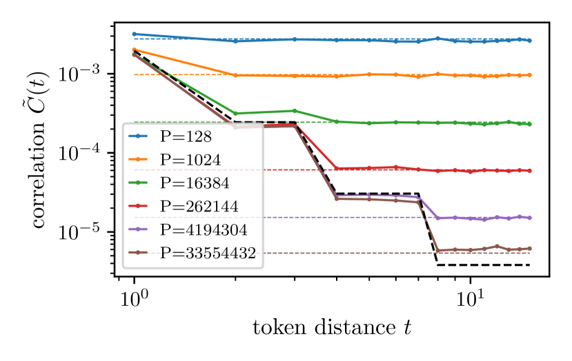
Figure 1: Left: Example of data generation according to the RHM, with depth $L\,{=}\,3$ and branching factor $s\,{=}\,2$. Starting from the root with $\ell\,{=}\,3$ and following the arrows, each level-$\ell$ symbol is replaced with a pair of lower-level symbols, down to the leaves with $\ell\,{=}\,0$. Right: Analytical correlation function of the RHM data (black dashed curve), measuring the strength of token-token correlations as a function of their distance. The stepwise decay mirrors the tree structure of the generative model. Empirical estimates (coloured, obtained from $P$ examples) initially follow the true correlation function, but then saturate due to the sampling noise (coloured dashed). As a result, a finite training set only allows for measuring correlations with the tokens up to a certain distance $t^{*}(P)$. Graphically, $t^{*}(P)$ corresponds to the highest value of $t$ where the empirical estimate matches the true correlation (e.g. $1$ for the orange and green curves, $3$ for the red curve).

Given a dataset of $d$-dimensional sequences of tokens in $\mathcal{V}$, we measure correlations via the token co-occurrences matrix, 

$$C_{i,j}(\mu,\nu)\coloneq\mathbb{P}\left\{X_{i}=\mu,X_{j}=\nu\right\}-\mathbb{P}\left\{X_{i}=\mu\right\}\mathbb{P}\left\{X_{j}=\nu\right\},$$ (5)

where $\mu$ and $\nu$ are arbitrary elements of the vocabulary $\mathcal{V}$ and $\mathbb{P}$ refers to the data distribution $P_{\mathbf{X}}$. Since the masked token is always the last in our setup, it is convenient to set $j\,{=}\,d$ and write $C_{i,d}$ as a function of the distance $t\,{=}\,|i-d|$ between the $i$-th and the masked token. Taking the root mean square over the vocabulary yields the correlation function:

$$\tilde{C}(t)\coloneq\left(\sum_{\mu,\nu\in\mathcal{V}}\left(C_{d-t,d}(\mu,\nu)\right)^{2}\right)^{1/2},$$ (6)

which measures the typical dependency between tokens as a function of their distance $t$. For RHM data with $m\,{=}\,v^{s-1}$, $P_{\bm{X}}$ is uniform over all the possible sequences of tokens in $\mathcal{V}$ and there are no correlations. If, instead, $m\,{<}\,v^{s-1}$, the correlations strength depends on the distance.  Fig. 1 shows an example with $L\,{=}\,4$, $s\,{=}\,2$, $v\,{=}\,32$ and $m\,{=}\,8$.

Correlations decay with distance.

The stepwise decay of $\mathcal{C}(t)$ mirrors the tree structure of the generative model. The masked token has the highest correlations with those belonging to the same $s$-tuple, as they were all generated by the same level-$1$ symbol (as in the blue box of Fig. 1, left). The second highest is with the tokens generated by the same level-$2$ symbol (orange box in the figure), and so on until the root. Formally, with $\ell\,{=}\,1,\dots,L$ denoting the height of the lowest common ancestor of the $d$-th and $(d-t)$-th tokens,

$$\tilde{C}(t)\,{=}\,\tilde{C}^{(\ell)}\quad\text{for}\quad t\,{=}\,s^{\ell-1},\dots,s^{\ell}-1,\quad\tilde{C}^{(1)}>\tilde{C}^{(2)}>\dots>\tilde{C}^{(L)}.$$ (7)

These $L$ plateau values can be determined analytically in the RHM by studying the statistics of the co-occurrences matrix over realisations of the generative model. Here we present a simple asymptotic argument, valid for large $m$ when the marginal distribution of each symbol is approximately uniform [20]. In this limit, the joint probability $\mathbb{P}\left\{X_{d-t}=\mu,X_{d}=\nu\right\}$ depends only on the sub-tree originated by the Lowest Common Ancestor (LCA) of $X_{d-t}$ and $X_{t}$ (e.g. the sub-tree in the orange box of Fig. 1, left for $d\,{=}\,8$ and $t\,{=}\,2,3$). As a result, $\mathbb{P}\left\{X_{d-t}=\mu,X_{d}=\nu\right\}$ can be written by first considering the probability $p_{c}$ for the choice of one LCA and a sequence of production rules determining $(X_{d-t},X_{d})$, then summing $p_{c}$ over all choices leading to the considered pair of observable symbols $(\mu,\nu)$. There are $v$ choices for the LCA, $m$ for the first production rule and $m^{2}$ ($m$ per branch) for each remaining generation, i.e. $vm^{2\ell-1}$ choices determining the pair $(X_{d-t},X_{d})$. Since the probabilities are uniform, $p_{c}\,{=}\,1/(vm^{2\ell-1})$. In addition, only (on average) $\bar{N}_{c}\,{=}\,(vm^{2\ell-1})/v^{2}$ of these choices leads to the specific pair of observable symbols ($\mu$,$\nu$). Therefore, by the central limit theorem,

$$\mathbb{P}\left\{X_{d-t}=\mu,X_{d}=\nu\right\}\simeq\sum_{\bar{N}_{c}\text{terms}}p_{c}\to\mathcal{N}(p_{c}\bar{N}_{c},p_{c}^{2}\bar{N}_{c}).$$ (8)

after removing the mean $\mathbb{P}\left\{X_{d-t}=\mu\right\}\mathbb{P}\left\{X_{d}=\nu\right\}\simeq 1/v^{2}$ and computing the standard deviation over $\mu$ and $\nu$,

$$\tilde{C}^{(\ell)}=\sqrt{p_{c}^{2}\bar{N}_{c}}=v^{-3/2}m^{1/2-\ell},$$ (9)

which is confirmed in Fig. 1, right. Notice that, after replacing $s^{\ell}$ with $t$, the $m^{-\ell}$ dependence on $\ell$ is approximated by a power-law decay $\tilde{C}(t)\sim t^{-\beta}$ with $\beta\,{=}\,\log{m}/\log{s}$.

Saturation due to finite training set.

When measuring the correlation function from a finite sample $\mathcal{X}_{P}$ of $P$ data, there is an additional contribution due to the sampling noise. The scenario is illustrated in Fig. 1, right: the empirical estimates $\hat{C}_{P}(t)$, shown as coloured lines for different values of $P$, begin by following the descent of the true correlation function $\tilde{C}(t)$. However, when approaching the sampling noise size $(v^{2}P)^{-1/2}$ (shown as dashed coloured lines in the figure and proved in App. B, they saturate. Combining the saturation with the values of the steps, we deduce that a finite training set allows for the resolution of correlations up to distance $t^{*}\,{=}\,s^{\ell^{*}}\,{-}\,1$ such that

$$\tilde{C}^{(\ell^{*})}>(v^{2}P)^{-1/2}>\tilde{C}^{(\ell^{*}+1)}.$$ (10)

Eq. 10 suggests that a language model trained from a finite set of examples can only extract information from the tokens within distance $t^{*}(P)$ from the last. In other words, a finite training set is equivalent to an effective context window of size $t^{*}(P)$. If $\tilde{C}\sim t^{-\beta}$, then $t^{*}(P)\sim{P^{1/2\beta}}$.

4 Self-supervised learning of the Random Hierarchy Model

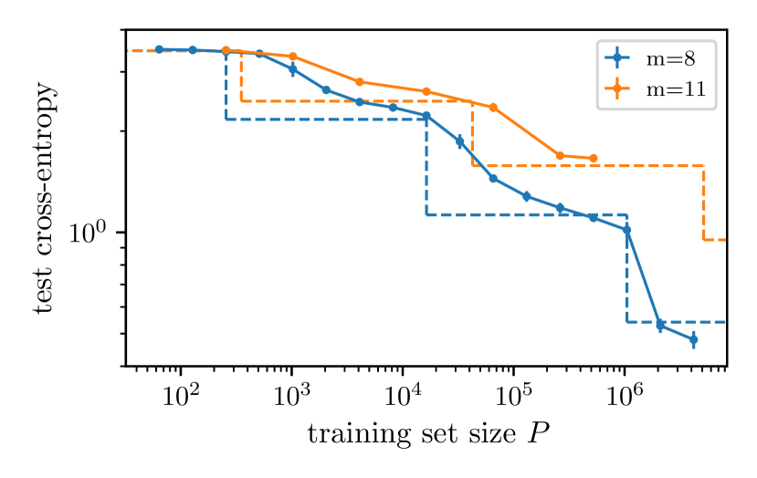
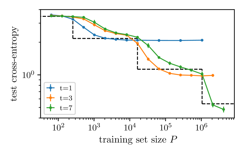
Figure 2: Left: Learning curves of depth-$3$ transformers trained on RHM data with $L\,{=}\,3$, $s\,{=}\,2$, $v\,{=}\,32$ and $m\,{=}\,8$ (blue) or $11$ (orange, both are averaged over $8$ independent realisations of the dataset and initialisations of the network), displaying a stepwise behaviour analogous to the correlation function. The vertical dashed lines mark the characteristic training set sizes $P_{k}$ at which the correlation with tokens at distances up to $t\,{=}\,s^{k}-1$ emerge from the sampling noise. Horizontal dashed lines represent (upper bounds on) the cross-entropy of the probability of the last token conditioned on the previous $s^{k}\,{-}\,1$, suggesting that the steps correspond to the model learning a progressively larger sub-tree of the data structure. Right: Learning curves of transformers for $m\,{=}\,8$ and different sizes $t$ of the context window. The saturation of the loss decay due to the finite context window highlights that the decay is entirely due to the ability to leverage a larger portion of the context window.

We now show how the correlations can be translated into a prediction of sample complexities that allow for a sequence of increasingly accurate approximations of the masked token probability, based on reconstructing the hidden variables of the generative tree. We then test these predictions in numerical experiments with deep networks.

4.1 Sequence of performance steps and sample complexities

Naive strategy: Imagine having a training set containing all the possible sequences of size $s^{\ell}$, masked token included. These sequences are exemplified by the strings of terminals at the bottom of the different coloured boxes of Fig. 1, left. Such a training set enables the reconstruction of the conditional probability $\mathbb{P}\left\{X_{d}|X_{d-s^{\ell}+1}=x_{d-s+1},\dots,X_{d-1}=x_{d-1}\right\}$. The resulting cross-entropy loss reads

$$\mathcal{L}_{\ell} =\displaystyle\mathbb{E}_{\mathbf{x}\sim P_{\bm{X}}}\left[-\log{\mathbb{P}\left\{X_{d}|X_{d-s^{\ell}+1}=x_{d-s+1},\dots,X_{d-1}=x_{d-1}\right\}}\right]$$

$$=\mathbb{E}_{\mathbf{x}\sim P_{\bm{X}}}\left[\log{N(x_{d-s^{\ell}+1},\dotsm x_{d-1})}\right],$$ (11)

where $N(x_{d-s^{\ell}+1},\dots,x_{d-1})$ denotes the number of possible values of the masked token depending on the observed effective context. For $\ell\,{=}\,0$, there is no restriction on the masked token value and this number equals $v$—the vocabulary size. For $\ell\,{=}\,1$, we can determine the average $\bar{N}_{1}\coloneq\mathbb{E}\left[N(x_{d-s+1},\dots,x_{d-1})\right]$ as follows. For each $s$-tuple $(x_{d-s+1},\dots,x_{d})$ there is at least one value of the mask compatible with the other $s-1$ symbols, i.e. $x_{d}$ itself. In addition, each of the remaining $v-1$ values $\mu_{d}\neq x_{d}$ has a probability $f$ of being compatible with the context, coinciding with the probability that the $s$-tuple $(x_{d-s+1},\dots,\mu_{d})$ is compatible with the production rules. This probability is given by $(mv-1)$, the number of $s$-tuples compatible with the production rules except $(x_{d-s+1},\dots,x_{d})$, over $(v^{s}-1)$, the total number of $s$-tuples except $(x_{d-s+1},\dots,x_{d})$. Therefore, $\bar{N}_{1}=1+(v-1)f=1+(v-1)(mv-1)/(v^{s}-1)$. For $\ell\,{>}\,1$, the average number $\bar{N}_{\ell}$ of symbols compatible with the context can be determined iteratively. The level-$\ell$ symbol generating the whole $s^{\ell}$-tuple can take any of the $v$ values, but the level-$\ell\,{-}\,1$ symbol above is now restricted to $\bar{N}_{\ell-1}$ values. By the previous argument, $\bar{N}_{\ell}=1+(v-1)(m\bar{N}_{\ell-1}-1)/(v^{s}-1)$. Due to the concavity of the logarithm, we can bound the test loss of subsection 4.1 with $\bar{\mathcal{L}}_{\ell}\,{=}\,\log{\bar{N}_{\ell}}$, i.e.

$$\bar{\mathcal{L}}_{\ell}=\log{\left(\frac{v^{s}-v}{v^{s}-1-m(v-1)}+\frac{(v^{s}-mv)(v-1)}{v^{s}-1-m(v-1)}\left(\frac{m(v-1)}{v^{s}-1}\right)^{\ell}\right)}\xrightarrow[]{}\log{\left(1+v\left(\frac{m}{v^{s-1}}\right)^{\ell}\right)},$$ (12)

where the limit is realised for $v,m\,{\gg}\,1$ and $m/v^{s-1}\ll 1$. In this limit, the test loss converges to $0$ for large $\ell$. However, since the number of possible sequences of size $s^{\ell}$ is $vm^{\frac{s^{\ell}-1}{s-1}}$, exponential in $t\,{=}\,s^{k}\,{-}\,1$, this strategy is cursed by the context dimensionality.

Reconstruction of the hidden variables: Using correlations, the same sequence of loss values can be obtained with a sequence of sample complexities that are only polynomial in the context size. Consider, for instance, the pair $(\mu^{\text{\tiny(0)}}_{5},\mu^{\text{\tiny(0)}}_{6})$ in Fig. 1. The correlation between any such pair and the masked token depends only on the level-$1$ hidden variable $\mu^{\text{\tiny(1)}}_{3}$. Thus, pairs displaying the same correlations can be grouped as descendants of the same hidden variable. As shown in [20] in the context of classification, gradient descent can perform such grouping by building a hidden representation of pairs that only depends on $\mu^{\text{\tiny(1)}}_{3}$. This representation is convenient since, once $\mu^{\text{\tiny(1)}}_{3}$ is known, the masked symbol is independent of the pair $(\mu^{\text{\tiny(0)}}_{5},\mu^{\text{\tiny(0)}}_{6})$. This strategy requires enough training data to resolve correlations between the masked token and the adjacent $s$-tuples of observable tokens. These correlations can be computed by replacing the $d-t$-th token with its $s$-tuple in the argument leading to Eq. 9. As shown in App. C, the replacement reduces correlation plateaus and sampling noise by the same factor. Therefore, the condition for the resolution of correlations with $s$-tuples at distance $s\,{<}\,t\,{<}\,s^{2}-1$ is also given by Eq. 10, which implies $P\,{>}\,P_{2}\,{=}\,vm^{3}$.

By iterating this argument we get a sequence of sample complexities $P_{\ell}$ that allow for resolving correlations between the masked token and $s$-tuples at a distance $s^{\ell-1}\,{<}\,t\,{<}\,s^{\ell}-1$,

$$P_{\ell}\,{=}\,vm^{2\ell-1}.$$ (13)

For instance, in the case illustrated in Fig. 1, left, the correlations of the pairs $(\mu^{\text{\tiny(0)}}_{1},\mu^{\text{\tiny(0)}}_{2})$ and $(\mu^{\text{\tiny(0)}}_{3},\mu^{\text{\tiny(0)}}_{4})$ with the masked token can be used to reconstruct the pair of hidden symbols $(\mu^{\text{\tiny(1)}}_{1},\mu^{\text{\tiny(1)}}_{2})$. The hidden symbols have a higher correlation with the masked token than their children. Hence, as in the case of classification [20], a training set large enough to resolve correlations between observable and masked tokens also allows for resolving correlations with the hidden symbols. These correlations yield a representation of higher-level hidden symbols (e.g. $\mu^{\text{\tiny(2)}}_{1}$ for $(\mu^{\text{\tiny(1)}}_{1},\mu^{\text{\tiny(1)}}_{2})$ in the figure), which, in turn, enables the reconstruction of $\mathbb{P}\left\{X_{d}|X_{d-s^{\ell}+1}=x_{d-s+1},\dots,X_{d-1}=x_{d-1}\right\}$.

4.2 Stepwise behaviour of empirical learning curves

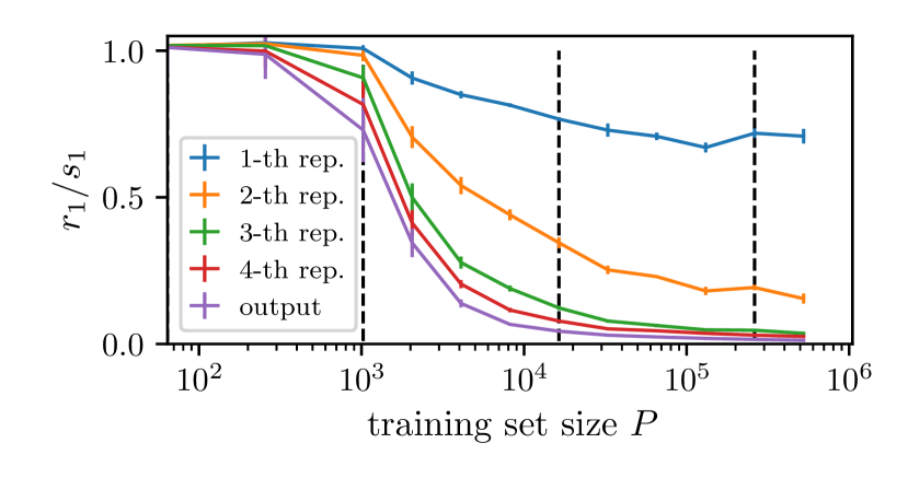
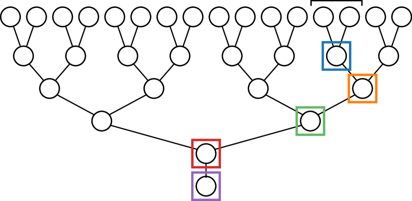
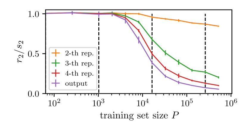
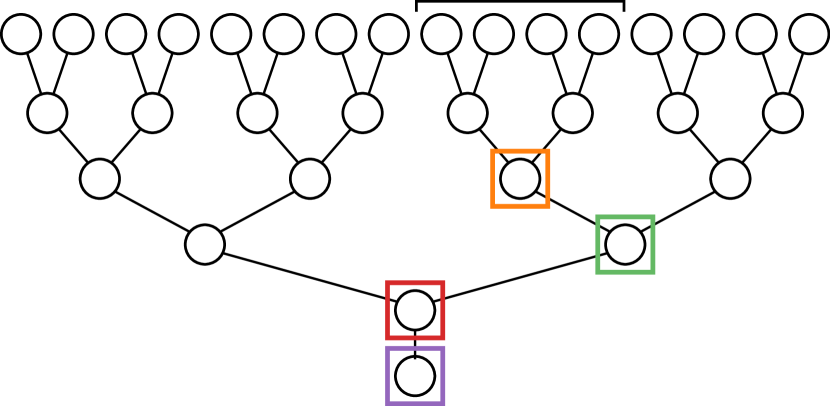
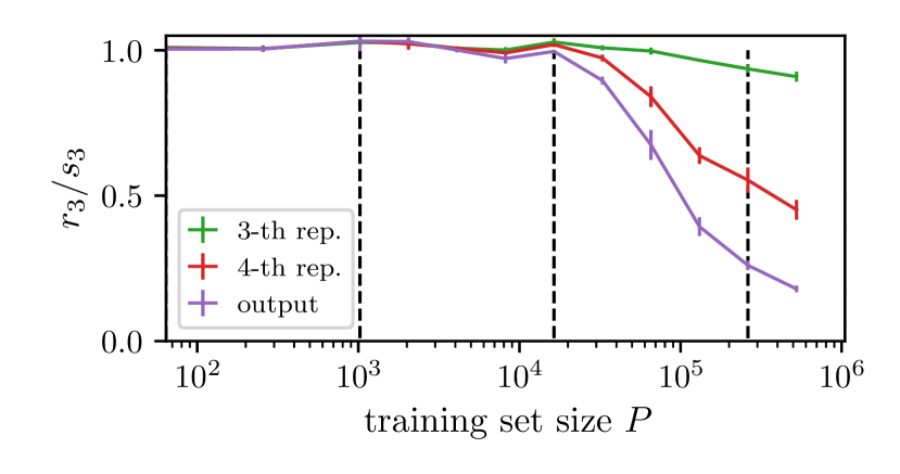
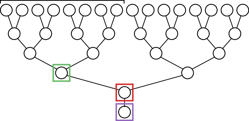
Figure 3: Relative sensitivity $r_{\ell}/s_{\ell}$ of the representation of trained depth-$4$ CNNs (sketched on the right panels) for input transformations (the affected tokens are indicated by the black horizontal segments on the right panels) corresponding to resetting the production rule emanating from a given level-$\ell$ variable ($\ell=1,2,3$ for top, centre and bottom), as a function of training set size $P$. Colours represent the layer of the representation, as indicated in the key and by the squares on the right panels. The CNNs are trained on RHM data with $L\,{=}\,4$, $s\,{=}\,2$, $v\,{=}\,16$, $m\,{=}\,4$. Vertical dashed lines mark the sample complexities $P_{\ell}$ of Eq. 13. The drop of the curves from $\simeq 1$ to $\simeq 0$ around $P_{\ell}$ signals that the trained representations only encode for the relevant level-$\ell$ symbol when $P\,{>}\,P_{\ell}$.

Fig. 2, left, compares the learning curves of deep transformers with the sample complexities $P_{k}$ of Eq. 13 (vertical dashed lines in the figure) and the test loss upper bounds $\bar{\mathcal{L}}_{k}$ of Eq. 12 (horizontal dashed lines). The learning curves display steps whose position and magnitude are in good qualitative agreement with our predictions for both architectures. Additional experiments that support the quantitative scaling of the sample complexities $P_{1}$ and $P_{2}$ with $m$ are shown in App. D.

Fig. 2, right, shows the learning curves of models trained on a reduced context window. In this setting, our description correctly predicts the saturation of the loss due to the finite context window size $t$: with $t\,{=}\,s^{\ell}-1$, the model can only learn the level-$\ell$ hidden variable above the masked token, thus follow only the first $\ell$ of the $L$ steps of Eq. 12.

Let us remark that, as shown in App. D, the learning curves are qualitatively similar for CNNs, despite a noticeable quantitative dependence on architecture and context size $t$. These differences are not captured by the analysis of subsection 4.1, although, in some cases, they can be rationalised using results from the theory of shallow neural networks. We discuss these aspects in detail in App. D.

4.3 Emergence of hierarchical representations of the data structure

We now study the hidden representations of models trained on RHM data to show that, as the training set size increases, these representations encode for deeper hidden variables. More specifically, we show that certain representations depend only on specific, high-level hidden variables of a datum’s tree structure, thus becoming insensitive to the entire subtree emanating from this hidden variable. For the sake of interpretability, we consider deep convolutional networks (CNNs) with architecture matched to the data structure, represented schematically in the graphs on the right of Fig. 3 (further details in subsection A.1). To probe representations we introduce two sets of transformations. Given a datum and the associated tree ( Fig. 1, left), consider the $i$-th level-$\ell$ symbol $\mu^{\text{\tiny($\ell$)}}_{i}$: $\mathcal{S}_{\ell,i}$ replaces it with another one randomly chosen from the vocabulary, whereas $\mathcal{R}_{\ell,i}$ resets the choice of the production rule emanating from $\mu^{\text{\tiny($\ell$)}}_{i}$. Both transformations alter the subtree originating from $\mu^{\text{\tiny($\ell$)}}_{i}$ (e.g. the subtree within the orange box of Fig. 2, left for $\ell\,{=}\,2$ and $i\,{=}\,2$), affecting $s^{\ell}$ observable tokens. However, $\mathcal{R}_{\ell,i}$ preserves the hidden symbols that generated the subtree. Therefore, a hidden representation that encodes only the $i$-th level-$\ell$ hidden symbol will be invariant to $\mathcal{R}_{\ell,i}$ but not to $\mathcal{S}_{\ell,i}$.

We define hidden representations $h_{\ell}(x)$ (hidden nodes of the network’s graphs in Fig. 3) as the sequence of pre-activations in a given layer $\ell$ (depth of the node in the tree), standardised over the dataset (i.e. centred around the mean and scaled by the standard deviation). For CNNs, representations carry a spatial index $j\,{=}\,1,\dots,s^{L-\ell}$ (horizontal position of the node within the layer) and a channel index. We measure the sensitivity to $\mathcal{R}$ or $\mathcal{S}$ via the cosine similarity between original and transformed representations, i.e.

$$r_{\ell,i}(h)=\mathbb{E}_{x\sim P_{\bm{X}}}\left[h_{\ell^{\prime},j}(x)\cdot h_{\ell^{\prime},j}(\mathcal{R}_{\ell,i}x)\right],s_{\ell,i}(h)=\mathbb{E}_{x\sim P_{\bm{X}}}\left[h_{\ell^{\prime},j}(x)\cdot h_{\ell^{\prime},j}(\mathcal{S}_{\ell,i}x)\right],$$ (14)

where the $\cdot$ symbol denotes the scalar product over the channels. In order to leave the masked token unaltered, we always apply the transformations to the penultimate hidden symbol of the level, i.e. $i\,{=}\,s^{L-\ell}-1$. Hence, from now on, we omit the spatial index $i$. The left column of Fig. 3 reports the ratio $r_{\ell}/s_{\ell}$ for the hidden representations of a deep CNN trained on RHM data. Each row refers to the level of the data transformations. The group of observable tokens affected by the transformation is highlighted by horizontal square brackets in the right panels. The drop of $r_{\ell}/s_{\ell}$ from $\approx 1$ to $\approx 0$ signals that a representation depends on the corresponding level-$\ell$ hidden variable, but not on the other variables in the associated subtree.  These drops occur at the same training set sizes $P_{\ell}$ as the test loss steps, highlighted in the figures with vertical dashed lines. This result confirms that, as $P$ increases, trained models learn a deeper representation of the tree structure of the data.

5 Conjecture and test on real language data

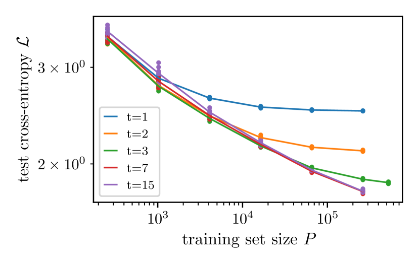
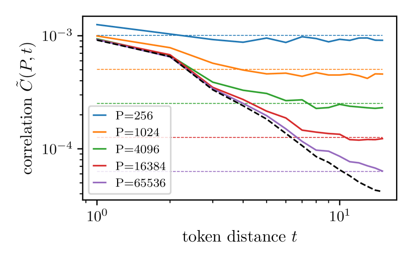
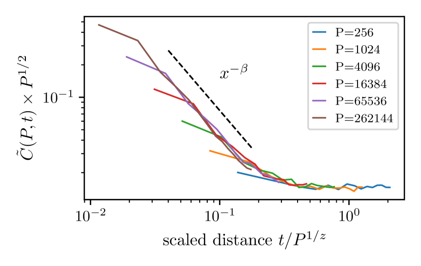
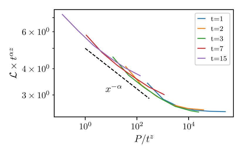
Figure 4: Top, Left: Test losses of $3$-layers transformers trained on $(t\,{+}\,1)$-characters blocks of the tiny-Shakespeare dataset [30], with $t$ as in the key. The decay of the loss saturates to some $t$-dependent value, indicating that performance improves with $P$ because the model can use information from a larger context window. Top, Right: Empirical estimates of $\tilde{C}(P,t)$ versus token distance $t$, for different training set sizes $P$ as in the key. The curves initially follow the true correlation $\tilde{C}(t)$ (black dashed), but then saturate due to the sampling noise (coloured dashed). Bottom, Left: The curves $\tilde{C}(P,t)$ collapse when rescaling correlations by the sampling noise size $P^{-1/2}$ and $t$ by the characteristic distance $t^{*}(P)\sim P^{1/z}$, with $z\simeq 2.8$. Bottom, Right: As predicted by our conjecture, the losses collapse when rescaled according to Eq. 16 with the same $z$ as the correlation functions.

We conjecture that the relationship between training set size, correlations and effective context window holds beyond our synthetic dataset.

Conjecture:

“If the token correlation function decays with the token distance, then a language model trained to predict the next token from a finite set of $P$ examples can only extract relevant information from an effective context window of $P$-dependent size $t^{*}(P)$.”

We test this conjecture in a dataset consisting of a selection of lines from Shakespeare’s plays [30]. We adopt a character-level tokenisation, resulting in a dataset of over $10^{6}$ tokens. We then extract sequences of $t$ consecutive characters and train a BERT-like deep transformers in the setup of section 2—further details of architecture and training are in subsection A.3. The results of our test are reported in Fig. 4. First, with a large context window, the test loss follows the empirical scaling law $\mathcal{L}\sim P^{-\alpha}$. However, the learning curve levels off at some characteristic scale $P$ that grows with the size $t$ of the context window (top, left). This phenomenon can be explained via the correlation function, which decays as a power of the distance $\tilde{C}(t)\sim t^{-\beta}$, with $\beta\simeq 1.4$ (top, right). Empirical estimates $\tilde{C}(P,t)$ of $\tilde{C}(t)$ saturate when reaching the sampling noise scale $\sim P^{-1/2}$: following the analysis of section 3, this behaviour results in an effective context window size $t^{*}(P)$. $t^{*}(P)$ can be determined graphically as the value of $t$ where the true correlation function intersects the sampling noise scale (bottom, left):

$$\tilde{C}(t^{*})\sim P^{-1/2}\Rightarrow t^{*}(P)\sim P^{1/z},\quad\text{ with }z\,{=}\,2\beta\,{\simeq}\,2.8.$$ (15)

By inverting $t^{*}(P)$ we get a characteristic training set size $P^{*}(t)$ where the training set allows for resolving correlations at all distances $t^{\prime}\,{<}\,t$, $P^{*}(t)\sim t^{z}$. Remarkably, this scale predicts the value of $P$ where the scaling laws level off (bottom, right). Paired with the empirical power-law scaling with $P$, our conjecture leads to the following context-dependent scaling hypothesis:

$$\mathcal{L}(P,t)=t^{-\alpha z}f\left(\frac{P}{t^{z}}\right)=P^{-\alpha}g\left(\frac{P}{t^{z}}\right),$$ (16)

with $g(x)$ constant for $x\,{\ll}\,1$ and $g(x)\sim x^{\alpha}$ for $x\,{\gg}\,1$. The collapse reported in the bottom right panel of Fig. 4 quantitatively confirms this hypothesis and our previous conjecture.

6 Conclusions

We proposed a conceptual framework for understanding the learning curves of language acquisition via deep learning. In our picture, increasing the number of data allows for the resolution of a longer range of correlations. These correlations, in turn, can be exploited to build a deeper representation of the data structure, thus improving next-token prediction performance. This scenario is consistent with known observations on language models, such as the emergence of skills at specific training set sizes [18, 31, 32, 33] and the steady improvement of the generalisation performance despite the high dimensionality of the problem. To the best of our knowledge, this is the first description of how generalisation abilities improve with the size of the training set in a setting where learning data features is crucial, with many previous works focusing on kernel limits [34, 35, 36, 37, 38]. Furthermore, our analysis makes novel predictions, including how the context window should enter the scaling description of learning curves, which we confirmed empirically on a real language dataset. Looking forward, self-supervised learning techniques can be used to build hierarchical representations of different data types, including videos and world models for autonomous agents [39]. It would be interesting to test our conjecture in these settings.

Limitations. Due to the fixed geometry of the data tree, the correlation functions and learning curves of our model data display a stepwise behaviour that depends on the specific position of the masked token. Therefore, relaxing the fixed-tree constraint is a necessary step for describing the smooth decay observed in real data. In addition, there is no proof of the connection between the strategy illustrated in subsection 4.1 and the sample complexity of deep neural networks trained with gradient descent and its variants. Such a proof would require a formal description of the training dynamics of deep networks, which is beyond the current status of the field. This description would also capture the discrepancies presented in App. D.

Appendix A Details of the experiments

Our experiments on RHM data consider both Deep CNNs tailored to the RHM structure and simple transformers made by stacking standard Multi-Head Attention layers. Our experiments on the tiny-Shakespeare dataset consider deep, encoder-only transformers, where Multi-Head Attention layers are interspersed with residual connections, layer normalization and two-layer perceptrons. All our experiments were performed on a cluster of NVIDIA V100 PCIe 32 GB GPUs (2×7TFLOPS). Single experiments require up to 20 GPU hours for the largest models ($\approx 10\times 10^{6}$) with the largest training set sizes ($\approx 4\times 10^{6}$), with an estimated total (including hyperparameter tuning) of $6,000$ GPU hours. We provide architecture and training details for all of these models below.

A.1 Deep CNNs (RHM)

The deep CNNs we consider are made by stacking standard convolutional layers. To tailor the network to the structure of the data generative model, we fix both the stride and filter size of these layers to $s$. Since each layer reduces the spatial dimensionality by a factor $s$, the input size $d$ must be an integer power of $s$ and the CNNs depth equals $\log{d}/\log{s}$.

We use the Rectified Linear Unit (ReLU) $\sigma(x)\,{=}\,\text{max}\left(0,x\right)$ as activation function, set the number of channels to $H$ for each layer, and consider the maximal update parametrization [40], where the weights are initialised as random gaussian variables with zero mean and unit variance, all the hidden layers but the last are rescaled by a factor $H^{-1/2}$, whereas the last is rescaled by ${H}^{-1}$. This factor causes the output at initialization to vanish as $H$ grows, which induces representation learning even in the $H\to\infty$ limit. In practice, $H$ is set to $256$ for Fig. 3, $512$ for Fig. 5, left and Fig. 8, $1024$ for Fig. 5, right, $512$ for Fig. 6 and Fig. 7. Increasing the number of channels does not affect any of the results presented in the paper.

Deep CNNs are trained with SGD, with the learning rate set to $H$ to compensate for the factor of $H^{-1}$. A cosine annealing scheduler reduces the learning rate by $10$ within the first $100$ training epochs. The batch size is set to the minimal size allowing convergence, where we define convergence as the training cross-entropy loss reaching a threshold value of $10^{-3}$. We use a validation set of size $2^{15}$ to select the model with the best validation loss over the training trajectory.

A.2 Multi-layer self-attention (RHM)

The deep Transformers that we train on RHM data are made by stacking standard Multi-Head Attention layers [41], without residuals, layer normalization and multi-layer perceptron in between. We found that the removed components do not affect the model’s performance on data generated from the RHM. Each layer has the same number of $n_{h}$ and embedding dimension set to $n_{h}\times v$, with $v$ the vocabulary size. We set $n_{h}\,{=}\,16$ and notice no significant change in performance in the range $n_{h}\,{=}\,4\div 64$. The input dimension is adapted to the embedding dimension via a learnable linear projection, to which we add learnable positional encodings.

Multi-layer self-attention networks are trained with the Adam optimizer, with a warmup scheduler bringing the learning rate to $10^{-2}$ within the first $10$ training epochs. As for CNNs, the batch size is set to the lowest value that allows for convergence.

A.3 Encoder-only Transformer (tiny-Shakespeare)

The architectures trained on the tiny-Shakespeare dataset have the same structure as BERT [8]. With respect to the multi-layer self-attention of the previous section, they include additional token-wise two-layer perceptions (MLPs) after each self-attention layer, together with layer normalization operations before the attention layer and the MLP and residual connections. The training procedure is the same as for multi-layer self-attention.

For this dataset, we set the number of heads to $n_{h}\,{=}\,8$, the embedding dimension to $d_{e}\,{=}\,256\,{=}\,32\times n_{h}$, the size of the MLP hidden layer to $1024\,{=}\,4d_{e}$, and the number of layers to $3$. Increasing the number of layers or the number of heads does not affect the results presented in this paper.

Appendix B Sampling noise in the empirical correlation function

In this appendix, we prove that the sampling noise on empirical correlation functions of RHM data has a characteristic size $(v^{2}P)^{-1/2}$.

Let us denote, to ease notation, $\mathbb{P}\left\{X_{d-t}=\mu,X_{d}=\nu\right\}$ with $p(\mu,\nu)$, $\mathbb{P}\left\{X_{d-t}=\mu\right\}$ with $p(\mu)$ and $\mathbb{P}\left\{X_{d-t}=\mu\right\}$ with $p(\nu)$. When measuring probabilities from the frequency of observations over $P$ i.i.d. samples,

$$\hat{p}(\mu,\nu)=\frac{1}{P}\sum_{k=1}^{P}\delta(X_{k,d-t}\,{=}\,\mu,X_{k,d}\,{=}\,\nu),$$ (17)

where $\hat{.}$ denotes the empirical estimate and the indicator variable $\delta$ is $1$ with probability $p(\mu,\nu)$ and $0$ otherwise. With $\delta$ having finite mean and variance, by the central limit theorem,

$$\hat{p}(\mu,\nu)\xrightarrow{P\to\infty}p(\mu,\nu)+\sqrt{\frac{p(\mu,\nu)(1-p(\mu,\nu))}{P}}\xi,$$ (18)

where $\xi$ is a Gaussian random variable with zero mean and unitary variance. Analogously,

$$\hat{p}(\mu)\xrightarrow{P\to\infty}p(\mu)+\sqrt{\frac{p(\mu)(1-p(\mu))}{P}}\zeta_{1},$$

$$\hat{p}(\nu)\xrightarrow{P\to\infty}p(\nu)+\sqrt{\frac{p(\nu)(1-p(\nu))}{P}}\zeta_{2},$$ (19)

where $\zeta_{1}$ and $\zeta_{2}$ are also Gaussian random variables with zero mean and unitary variance, correlated with each other and with $\xi$.

As a result, the empirical estimation of $C_{t}(\mu,\nu)$ reads

$$\hat{C}_{t}(\mu,\nu)\xrightarrow{P\to\infty}p(\mu,\nu)- p(\mu)p(\nu)+\sqrt{\frac{p(\mu,\nu)(1-p(\mu,\nu))}{P}}\xi$$

$$- p(\mu)\sqrt{\frac{p(\nu)(1-p(\nu))}{P}}\zeta_{2}-p(\nu)\sqrt{\frac{p(\mu)(1-p(\mu))}{P}}\zeta_{1}.$$ (20)

In the limit of large $v$ and $m$, where $p(\mu,\nu)$ converges to $1/v^{2}$ plus vanishingly small fluctuations and $p(\mu)$, $p(\nu)$ converge to $1/v$ plus vanishingly small fluctuations, the dominant noise contribution is the one of $\xi$, with standard deviation

$$\sqrt{\frac{p(\mu,\nu)(1-p(\mu,\nu))}{P}}\xrightarrow{v,m\gg 1}\sqrt{\frac{1}{v^{2}P}}.$$ (21)

The correlation function $\tilde{C}(t)$ is the standard deviation of $C_{t}(\mu,\nu)$ over vocabulary entries. Hence, the sampling noise on $C_{t}(\mu,\nu)$ results in an additive factor of $(v^{2}P)^{-1/2}$.

Appendix C Correlations between mask and tuples of observable tokens

In this section, we generalise the argument leading to Eq. 9 of the main text to correlations between the masked token and $s$-tuples of observable tokens.

In general, single- and two-token probabilities can be written as products of probabilities over the single production rules. E.g., for the single-token probability,

$$\mathbb{P}\left\{X_{i}\,{=}\,\mu\right\}=\sum_{\mu_{1},\dots,\mu_{L}=1}^{v}p^{(1)}_{i_{1}}(\mu|\mu_{1})\dots p^{(L)}_{i_{L}}(\mu_{L-1}|\mu_{L})p^{(L+1)}(\mu_{L}),$$ (22)

where

• the indices $i_{1},\dots,i_{L}$ identify the branches of the tree to follow when going from the root to the $i$-th leaf;

• $p^{(\ell)}_{i_{\ell}}(\mu_{\ell-1}|\mu_{\ell})$ denotes the probability of choosing, among the available production rules starting from $\mu_{\ell}$, one that has the symbol $\mu_{\ell-1}$ on the $i_{\ell}$-th position of the right-hand size;

• $p^{(L)}(\mu_{L})$ denotes the probability of selecting the symbol $\mu_{L}$ as the root, $1/v$ for our model.

These decompositions arise naturally due to the connection between probabilistic context-free grammars and Markov processes. For the joint probability of two tokens at distance $s^{\ell-1}\,{<}\,t_{\ell}\,{<}\,s^{\ell}-1$, such that the lowest common ancestor is a level-$\ell$ hidden symbol,

$$\mathbb{P}\left\{X_{i}\,{=}\,\mu,X_{j}\,{=}\,\nu\right\}=\sum_{\begin{subarray}{c}\mu_{1},\dots,\mu_{\ell}=1\\ \nu_{1},\dots,\nu_{\ell-1}=1\end{subarray}}^{v}\sum_{\mu_{\ell}=1}^{v}p^{(1)}_{i_{1}}(\mu|\mu_{1})p^{(1)}_{j_{1}}(\nu|\nu_{1})\dots p^{(\ell)}_{i_{\ell},j_{\ell}}(\mu_{\ell-1},\nu_{\ell-1}|\mu_{\ell})p^{(\ell+1)}(\mu_{\ell}).$$ (23)

Both in Eq. 22 and Eq. 23 simplify when replacing $\mu$ with a whole $s$-tuple of observable symbols $\bm{\mu}_{j}\,{=}\,(\mu_{1+(j-1)s},\dots,\mu_{js})$ for some $j\,{=}\,1,\dots,s^{L-1}$. The simplification arises because the level-$1$ rule probability $p^{(1)}(\bm{\mu}_{j}|\mu_{1})$, is uniform and equal to $1/m$ if the production rule $\mu_{1}\to\bm{\mu}_{j}$ exists, $0$ otherwise. Then, the sum over $\mu_{1}$ selects the only level-$1$ symbol that generates the tuple $\bm{\mu}_{j}$. As a result, one is left with a probability represented by a smaller tree, where the $s$ leaves representing $\bm{\mu}_{j}$ are pruned, and an additional factor of $1/m$.

In the case of the joint tuple-token probability, following the argument to Eq. 9, the probability of a specific choice remains the same, $p_{c}\,{=}\,1/(vm^{2\ell-1})$ but the average number of choices leading to the tuple-token pair ($\bm{\mu}_{j},\nu$) is reduced by $m$, $\bar{N}_{c}\,{=}\,vm^{2\ell-1}/(v^{2}m)$. Therefore,

$$\tilde{C}^{(\ell)}_{\text{tuple}}=\sqrt{p^{2}_{c}\bar{N}_{c}}=v^{-3/2}m^{-\ell},$$ (24)

equal to $\tilde{C}^{(\ell)}/\sqrt{m}$ with $\tilde{C}^{\ell}$ as in Eq. 9. Crucially, since the average joint tuple-token probability is $1/(v^{2}m)$, the sampling noise size, obtained via the calculations of App. B, is also reduced by a factor of $\sqrt{m}$, leaving the condition of Eq. 10.

Appendix D Experiments on deep CNNs and scaling of the loss steps

In this section, we present empirical learning curves of Deep CNNs trained for last-token prediction (details in subsection A.1). In particular, we discuss discrepancies between these curves and those of Transformers (Fig. 2) in subsection D.1, verify the scaling with $m$ of the first two steps of Eq. 13 in subsection D.2, then discuss the role of the context window size $t$ in subsection D.3.

D.1 Differences between Transformers and deep CNNs

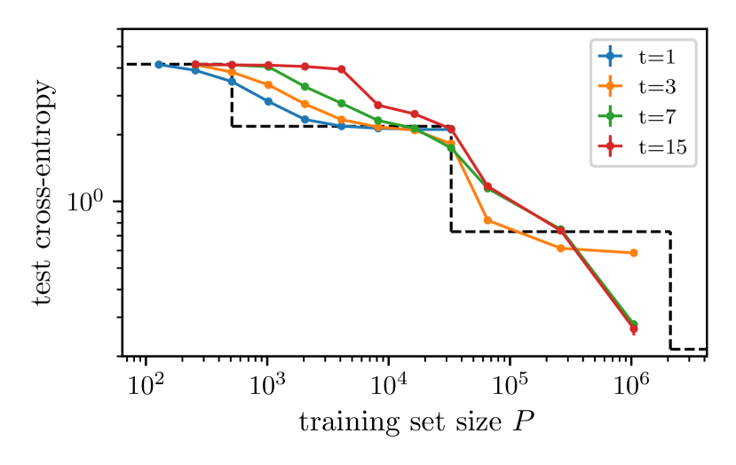
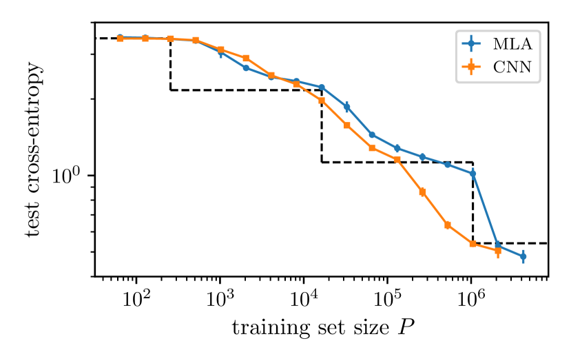
Figure 5: Left: Learning curves of deep CNNs trained on RHM data with $L\,{=}\,4$, $s\,{=}\,2$, $v\,{=}\,64$ and $m\,{=}\,8$ for different sizes $t$ of the context window. The network’s depth is fixed to $\log{s^{L}}/\log{(t+1)}$ and the blacked dashed line represents predictions from Eq. 13 and Eq. 12. The finite context window causes saturation of the loss as predicted by our analysis. However, the third step occurs with less training data than $P_{3}$. Right: This discrepancy is highlighted by the comparison of Transformer and deep CNN learning curves, here for $L\,{=}\,4$, $s\,{=}\,2$, $v\,{=}\,64$ and $m\,{=}\,8$.

The learning curves of deep CNNs are qualitatively similar to those of transformers, but also present apparent quantitative differences, as shown in Fig.5. Specifically, a noticeable difference is the sample complexity of the third step $P_{3}$. This difference is possibly due to favorable implicit biases of CNNs, such as weight sharing. Indeed after learning the penultimate level-$1$ feature in the second step, weight sharing would facilitate learning the other level-$1$ features along the entire data. This effect may affect the sample complexity of the third step and the subsequent ones. However, the third step occurs for large values of the training set size, and we cannot investigate this issue systematically in numerical experiments.

D.2 Scaling with the number of production rules $m$

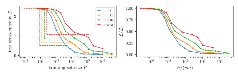
Figure 6: Learning curves of depth-$3$ CNNs trained on RHM data with $L\,{=}\,3$, $s\,{=}\,3$, $v\,{=}\,11$ and $m$ as in the key. Dashed curves highlight our prediction for the first step. In the right panel, the first step is made to collapse by rescaling $P$ with $P_{1}$ and $\mathcal{L}$ with $\mathcal{L}_{0}\,{=}\,\log{v}$. The collapse confirms our prediction on the behaviour of $P_{1}$ with $m$.

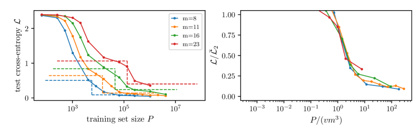
Figure 7: Same as Fig. 6 but focused on the second step, highlighted on the left by dashed curves. For the second step, collapse is achieved by rescaling $P$ with $P_{2}\,{=}\,vm^{3}$ and $\mathcal{L}$ with $\mathcal{L}_{1}$ from Eq. 12.

Fig. 6 and Fig. 7 show a scaling analysis of the behaviour of $P_{1}$ and $P_{2}$ from Eq. 13 in Deep CNNs. The collapse achieved when rescaling the number of data $P$ by $P_{\ell}$ and the test loss by the value before the jump $\mathcal{L}_{\ell-1}$ confirms this prediction.

D.3 Scaling with the size of the context window $t$

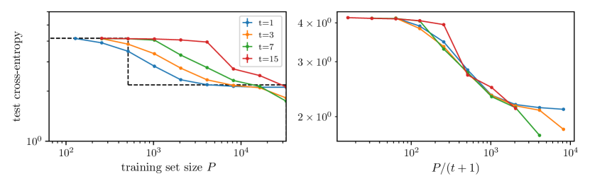
Figure 8: Zoom of the learning curves in Fig. 5, left, on the first step. The zoom highlights the dependence of the sample complexity on the context size $t$. The collapse of the curves on the right panel, achieved after dividing $P$ by $(t+1)$, reveals that $P_{1}\propto(t+1)$. This dependence is analogous to the sample complexity of regression of a target function depending on a low-dimensional linear projection of a large-dimensional input [42].

Similarly,  Fig. 8 shows a scaling analysis (for CNNs) of the behaviour of $P_{1}$ with the number of $s$-tuples in the input, proportional to $(t+1)$ with $t$ the size of the context window. The figure highlights a linear behaviour $P_{1}\propto(t+1)$ that our analysis does not capture. Nevertheless, this behaviour is expected from the theory of regression with one-hidden-layer neural networks [42]: when the target function depends on a small number of variables among $d$, the sample complexity is generically proportional to $d$. Proving this result by considering a single or a few steps of gradient descent, as often done in this literature, is an interesting work for the future.

References

- [1] Noam Chomsky. Aspects of the Theory of Syntax. The MIT Press, 50 edition, 1965.
- [2] Gerhard Jäger and James Rogers. Formal language theory: refining the chomsky hierarchy. Philosophical Transactions of the Royal Society B: Biological Sciences, 367(1598):1956–1970, 2012.
- [3] Robert C Berwick, Paul Pietroski, Beracah Yankama, and Noam Chomsky. Poverty of the stimulus revisited. Cognitive science, 35(7):1207–1242, 2011.
- [4] Nick C Ellis. Frequency effects in language processing: A review with implications for theories of implicit and explicit language acquisition. Studies in second language acquisition, 24(2):143–188, 2002.
- [5] Jenny R Saffran and Natasha Z Kirkham. Infant statistical learning. Annual review of psychology, 69:181–203, 2018.
- [6] Jenny R Saffran, Richard N Aslin, and Elissa L Newport. Statistical learning by 8-month-old infants. Science, 274(5294):1926–1928, 1996.
- [7] Jenny R Saffran. The use of predictive dependencies in language learning. Journal of Memory and Language, 44(4):493–515, 2001.
- [8] Jacob Devlin, Ming-Wei Chang, Kenton Lee, and Kristina Toutanova. Bert: Pre-training of deep bidirectional transformers for language understanding. In North American Chapter of the Association for Computational Linguistics, 2019.
- [9] Alec Radford, Karthik Narasimhan, Tim Salimans, and Ilya Sutskever. Improving language understanding with unsupervised learning. Technical report, OpenAI, 2018.
- [10] M. E. Peters, M. Neumann, L. Zettlemoyer, and W. Yih. Dissecting contextual word embeddings: Architecture and representation. In Ellen Riloff, David Chiang, Julia Hockenmaier, and Jun’ichi Tsujii, editors, Proceedings of the 2018 Conference on Empirical Methods in Natural Language Processing, pages 1499–1509, Brussels, Belgium, 2018. Association for Computational Linguistics.
- [11] I. Tenney, D. Das, and E. Pavlick. BERT rediscovers the classical NLP pipeline. In Anna Korhonen, David Traum, and Lluís Màrquez, editors, Proceedings of the 57th Annual Meeting of the Association for Computational Linguistics, pages 4593–4601, Florence, Italy, 2019. Association for Computational Linguistics.
- [12] C. D Manning, K. Clark, J. Hewitt, U. Khandelwal, and O. Levy. Emergent linguistic structure in artificial neural networks trained by self-supervision. Proceedings of the National Academy of Sciences, 117(48):30046–30054, 2020.
- [13] Zeyuan Allen-Zhu and Yuanzhi Li. Physics of language models: Part 1, context-free grammar. arXiv preprint arXiv:2305.13673, 2023.
- [14] Haoyu Zhao, Abhishek Panigrahi, Rong Ge, and Sanjeev Arora. Do transformers parse while predicting the masked word? arXiv preprint arXiv:2303.08117, 2023.
- [15] Sanjeev Arora and Anirudh Goyal. A theory for emergence of complex skills in language models. arXiv preprint arXiv:2307.15936, 2023.
- [16] Michael R Douglas. Large language models. arXiv preprint arXiv:2307.05782, 2023.
- [17] J. Kaplan, S. McCandlish, T. Henighan, T. B. Brown, B. Chess, R. Child, S. Gray, A. Radford, J. Wu, and D. Amodei. Scaling laws for neural language models. arXiv preprint arXiv:2001.08361, 2020.
- [18] Deep Ganguli, Danny Hernandez, Liane Lovitt, Amanda Askell, Yuntao Bai, Anna Chen, Tom Conerly, Nova Dassarma, Dawn Drain, Nelson Elhage, et al. Predictability and surprise in large generative models. In Proceedings of the 2022 ACM Conference on Fairness, Accountability, and Transparency, pages 1747–1764, 2022.
- [19] Rylan Schaeffer, Brando Miranda, and Sanmi Koyejo. Are emergent abilities of large language models a mirage? Advances in Neural Information Processing Systems, 36, 2024.
- [20] F. Cagnetta, L. Petrini, U. M. Tomasini, A. Favero, and M. Wyart. How deep neural networks learn compositional data: The random hierarchy model. arXiv preprint arXiv:2307.02129, 2023.
- [21] E. Mossel. Deep learning and hierarchal generative models. arXiv preprint arXiv:1612.09057, 2016.
- [22] Eran Malach and Shai Shalev-Shwartz. A provably correct algorithm for deep learning that actually works. Preprint at http://arxiv.org/abs/1803.09522, 2018.
- [23] Umberto Tomasini and Matthieu Wyart. How deep networks learn sparse and hierarchical data: the sparse random hierarchy model. arXiv preprint arXiv:2404.10727, 2024.
- [24] Antonio Sclocchi, Alessandro Favero, and Matthieu Wyart. A phase transition in diffusion models reveals the hierarchical nature of data. arXiv preprint arXiv:2402.16991, 2024.
- [25] Song Mei. U-nets as belief propagation: Efficient classification, denoising, and diffusion in generative hierarchical models. arXiv preprint arXiv:2404.18444, 2024.
- [26] E. Malach and S. Shalev-Shwartz. The implications of local correlation on learning some deep functions. In Advances in Neural Information Processing Systems, volume 33, pages 1322–1332, 2020.
- [27] Kabir Ahuja, Vidhisha Balachandran, Madhur Panwar, Tianxing He, Noah A Smith, Navin Goyal, and Yulia Tsvetkov. Learning syntax without planting trees: Understanding when and why transformers generalize hierarchically. arXiv preprint arXiv:2404.16367, 2024.
- [28] Adam Paszke, Sam Gross, Francisco Massa, Adam Lerer, James Bradbury, Gregory Chanan, Trevor Killeen, Zeming Lin, Natalia Gimelshein, Luca Antiga, Alban Desmaison, Andreas Kopf, Edward Yang, Zachary DeVito, Martin Raison, Alykhan Tejani, Sasank Chilamkurthy, Benoit Steiner, Lu Fang, Junjie Bai, and Soumith Chintala. PyTorch: An Imperative Style, High-Performance Deep Learning Library. In Advances in Neural Information Processing Systems, volume 32. Curran Associates, Inc., 2019.
- [29] Grzegorz Rozenberg and Arto Salomaa. Handbook of Formal Languages. Springer, 1997.
- [30] The unreasonable effectiveness of recurrent neural networks, 2015.
- [31] Jason Wei, Yi Tay, Rishi Bommasani, Colin Raffel, Barret Zoph, Sebastian Borgeaud, Dani Yogatama, Maarten Bosma, Denny Zhou, Donald Metzler, et al. Emergent abilities of large language models. arXiv preprint arXiv:2206.07682, 2022.
- [32] Tom Brown, Benjamin Mann, Nick Ryder, Melanie Subbiah, Jared D Kaplan, Prafulla Dhariwal, Arvind Neelakantan, Pranav Shyam, Girish Sastry, Amanda Askell, et al. Language models are few-shot learners. Advances in neural information processing systems, 33:1877–1901, 2020.
- [33] Aarohi Srivastava, Abhinav Rastogi, Abhishek Rao, Abu Awal Md Shoeb, Abubakar Abid, Adam Fisch, Adam R Brown, Adam Santoro, Aditya Gupta, Adrià Garriga-Alonso, et al. Beyond the imitation game: Quantifying and extrapolating the capabilities of language models. arXiv preprint arXiv:2206.04615, 2022.
- [34] Andrea Caponnetto and Ernesto De Vito. Optimal rates for the regularized least-squares algorithm. Foundations of Computational Mathematics, 7:331–368, 2007.
- [35] Stefano Spigler, Mario Geiger, and Matthieu Wyart. Asymptotic learning curves of kernel methods: empirical data versus teacher–student paradigm. Journal of Statistical Mechanics: Theory and Experiment, 2020(12), 2020.
- [36] Yasaman Bahri, Ethan Dyer, Jared Kaplan, Jaehoon Lee, and Utkarsh Sharma. Explaining neural scaling laws. arXiv preprint arXiv:2102.06701, 2021.
- [37] Francesco Cagnetta, Alessandro Favero, and Matthieu Wyart. What can be learnt with wide convolutional neural networks? In International Conference on Machine Learning, pages 3347–3379. PMLR, 2023.
- [38] Blake Bordelon, Alexander Atanasov, and Cengiz Pehlevan. A dynamical model of neural scaling laws. arXiv:2402.01092, 2024.
- [39] Yann LeCun. A path towards autonomous machine intelligence version 0.9. 2, 2022-06-27. Open Review, 62(1), 2022.
- [40] Greg Yang and Edward J Hu. Feature learning in infinite-width neural networks. arXiv preprint arXiv:2011.14522, 2020.
- [41] Ashish Vaswani, Noam Shazeer, Niki Parmar, Jakob Uszkoreit, Llion Jones, Aidan N Gomez, Łukasz Kaiser, and Illia Polosukhin. Attention is all you need. Advances in neural information processing systems, 30, 2017.
- [42] Yatin Dandi, Emanuele Troiani, Luca Arnaboldi, Luca Pesce, Lenka Zdeborová, and Florent Krzakala. The benefits of reusing batches for gradient descent in two-layer networks: Breaking the curse of information and leap exponents. arXiv preprint arXiv:2402.03220, 2024.