Stochastic Adversarial Networks for Multi-Domain Text Classification

Abstract

Adversarial training has been instrumental in advancing multi-domain text classification (MDTC). Traditionally, MDTC methods employ a shared-private paradigm, with a shared feature extractor for domain-invariant knowledge and individual private feature extractors for domain-specific knowledge. Despite achieving state-of-the-art results, these methods grapple with the escalating model parameters due to the continuous addition of new domains. To address this challenge, we introduce the Stochastic Adversarial Network (SAN), which innovatively models the parameters of the domain-specific feature extractor as a multivariate Gaussian distribution, as opposed to a traditional weight vector. This design allows for the generation of numerous domain-specific feature extractors without a substantial increase in model parameters, maintaining the model’s size on par with that of a single domain-specific extractor. Furthermore, our approach integrates domain label smoothing and robust pseudo-label regularization to fortify the stability of adversarial training and to refine feature discriminability, respectively. The performance of our SAN, evaluated on two leading MDTC benchmarks, demonstrates its competitive edge against the current state-of-the-art methodologies. The code is available at https://github.com/wangxu0820/SAN.

1 Introduction

Text classification has become a prominent area of focus within the field of Natural Language Processing (NLP) Khurana et al. (2023). The preceding decade has seen remarkable progress in deep learning, which has significantly propelled the capabilities of text classification Kowsari et al. (2019); Zhou et al. (2024). There’s a broad consensus that textual content is intrinsically domain-specific Wu et al. (2022b). This means a single word might evoke different sentiments in different contexts, leading to situations where a model, though effective in its training domain, may not yield optimal results in a new, untrained domain. The endeavor to amass extensive, labeled datasets for each specific domain often proves to be prohibitively expensive and challenging. Hence, it is imperative to explore and develop methods capable of harnessing knowledge from related domains to enhance the accuracy of classification in the target domain.

Multi-domain text classification (MDTC) is proposed to address the challenges highlighted above Li and Zong (2008); Hu and Wu (2024). Initial MDTC methods relied on domain-specific training and employed ensemble learning to produce final results Li et al. (2012); Wu and Huang (2015). However, the latest MDTC approaches, which utilize adversarial training Creswell et al. (2018); Ganin et al. (2016) and a shared-private scheme Bousmalis et al. (2016), deliver state-of-the-art performance. Adversarial training is utilized to align distinct domains, thereby facilitating the extraction of domain-invariant features. The shared-private scheme splits the latent space into two parts: a shared space that captures common features across domains, and a private space dedicated to capturing unique features specific to each domain. The domain-invariant features are expected to be both discriminative and transferable across domains, whereas the domain-specific features are intended to augment the distinctiveness and discriminative power of the feature set Bousmalis et al. (2016). However, these methods encounter a notable challenge. The shared-private framework requires the construction of domain-specific feature extractors for each domain, often involving complex neural networks. As new domains are introduced, the addition of numerous domain-specific extractors not only increases the model’s complexity but also impedes training convergence.

To address the challenges outlined, we introduce a novel framework termed Stochastic Adversarial Network (SAN), which employs a stochastic feature extractor as a replacement for multiple domain-specific feature extractors. This innovative extractor amalgamates an unlimited number of domain-specific extractors into prevailing MDTC methodologies without altering the model’s parameter count. In SAN, the conventional practice of utilizing specific weight points is replaced with a weight distribution, signifying the domain-specific feature extractors. Specifically, we employ a Gaussian distribution to model these extractors, with the mean symbolizing the central weight of the domain-specific feature extractor and the variance denoting the discrepancy across distinct domains. Throughout the training phase, the domain-specific feature extractor is periodically sampled from the prevailing distribution estimate, concurrently optimizing the Gaussian distribution. As a result, SAN is proficient in extracting domain-specific features from numerous domains utilizing a singular extractor. This approach circumvents the substantial escalation in the model’s parameter count that typically accompanies an increase in the number of domains, thereby ensuring the model size remains stable. To further refine model performance, we integrate domain label smoothing and robust pseudo-label regularization within the SAN. This integration promotes stability during adversarial training and enhances the discriminative capability of features. Empirical evaluations on two established MDTC benchmarks substantiate the efficacy of our SAN model, achieving competitive performance compared to state-of-the-art methods.

Our contributions are summarized as follows:

• We propose the Stochastic Adversarial Network (SAN) for MDTC, introducing an innovative stochastic feature extractor mechanism. This mechanism facilitates the extraction of domain-specific features across various domains through a singular stochastic extractor, substantially reducing the model’s parameter count. To the best of our knowledge, this study represents the first exploration of this matter in MDTC.

• We incorporate domain label smoothing and robust pseudo-label regularization techniques to stabilize the adversarial training and enhance the discriminability of the acquired features, respectively.

• Experimental results on two benchmark datasets highlight the effectiveness of the SAN approach relative to state-of-the-art methods. Additionally, a comparative analysis of the number of parameters and running time between SAN and conventional MDTC methods showcases the superior efficiency of our proposed approach.

2 Related Work

Adversarial Training (AT), initially conceptualized within the Generative Adversarial Network (GAN) framework for image generation, involves a dual mechanism: a generator creating images and a discriminator differentiating between synthesized and authentic images Creswell et al. (2018). Domain-Adversarial Neural Networks (DANN) extend AT to domain adaptation, training a feature extractor to counter a domain discriminator Ganin et al. (2016). The discriminator strives to identify source and target features, while the feature extractor seeks to produce domain-invariant features undetectable by the discriminator. Conditional Adversarial Neural Networks (CDAN) further advance this approach by applying multilinear conditioning to synchronize conditional distributions and incorporating entropy conditioning to aid transfer learning Long et al. (2018). However, AT is not without challenges; it’s prone to oscillatory gradients during training, leading to issues such as instability, delayed convergence, and mode collapse Arjovsky and Bottou (2017); Mescheder et al. (2018). To mitigate these issues, Wasserstein GAN leverages the earth mover distance for a more refined domain divergence measure Arjovsky et al. (2017). Moreover, Environment Label Smoothing (ELS) is employed to prompt the domain discriminator to generate soft probabilities, thereby enhancing AT’s stability Zhang et al. (2023).

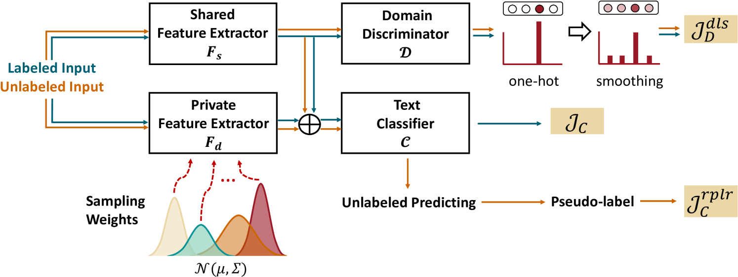
Figure 1: The architecture of the SAN method.

Stochastic Neural Network (SNN). The weight parameters of a neural network are typically treated as point estimates, limiting their ability to capture uncertainty and often resulting in overconfident predictions Blundell et al. (2015). To address this limitation, SNNs are proposed, which consider weight parameters as random variables sampled from specific distributions. For example, Bayesian Neural Networks (BNNs) Hernández-Lobato and Adams (2015); Wang and Yeung (2020) are widely used to represent intermediate outputs and final predictions as stochastic variables, providing richer representations. The Auto-Encoding Variational Bayes (AEVB) Kingma and Welling (2013) employs a Gaussian distribution to model latent variables in image inputs, serving as a form of data augmentation. Uncertainty-aware multi-modal BNNs Subedar et al. (2019) combine deterministic and variational layers for activity recognition, while DistributionNet Yu et al. (2019) models feature uncertainty in person re-identification using distributions. In unsupervised domain adaptation, the Stochastic Classifier Lu et al. (2020) leverages a Gaussian distribution to model classifier parameters.

Multi-domain text classifications (MDTC). MDTC aims to enhance overall classification accuracy by harnessing available resources from multiple domains Li and Zong (2008). Early MDTC methods employ transfer learning techniques to drive progress. The structural correspondence learning (SCL) Blitzer et al. (2006) method computes relationships between different pivot features to learn correspondences among them. The collaborative multi-domain sentiment classification (CMSC) Wu and Huang (2015) method trains two types of classifiers: a shared classifier for all domains and a set of domain-specific classifiers for each domain, combining their outputs for final results. Recent MDTC approaches commonly adopt the adversarial training and shared-private paradigm, leading to significant advancements. The domain separation network (DSN) Bousmalis et al. (2016) first introduces the shared-private paradigm for adversarial domain adaptation and empirically demonstrates that domain-unique features can enhance the discriminability of domain-invariant features. The adversarial multi-task learning (ASP-MTL) method Liu et al. (2017) applies adversarial training and the shared-private paradigm to MDTC. The multinomial adversarial networks (MAN) Chen and Cardie (2018) utilize the least square loss and negative log-likelihood loss to train the domain discriminator. The mixup regularized adversarial networks (MRANs) Wu et al. (2021b) propose domain and category mixup regularizers for MDTC. The maximum batch Frobenius norm (MBF) Wu et al. (2022b) method improves feature discriminability by maximizing the Frobenius norm of the intermediate feature matrix.

Our proposed SAN method contrasts with traditional MDTC techniques that deploy distinct domain-specific feature extractors for each domain. Instead, SAN adopts a parameter sampling strategy from a Gaussian distribution to instantiate domain-specific feature extractors. This innovative approach allows SAN to obtain domain-specific insights through a stochastic feature extractor, resulting in a significant reduction in the number of model parameters needed.

3 Method

The MDTC task can be formulated as follows: given $M$ domains $\left\{D_{i}\right\}^{M}_{i=1}$, each domain contains a small amount of labeled data $\mathbb{L}_{i}=\left\{\textbf{x}_{j},y_{j}\right\}_{j=1}^{l_{i}}$ and a large amount of unlabeled data $\mathbb{U}_{i}=\left\{\textbf{x}_{j}\right\}_{j=1}^{u_{i}}$. The primary objective of MDTC is to leverage these resources to enhance the average classification accuracy across all domains.

3.1 Adversarial Multi-Domain Text Classification

Adversarial training has garnered recognition for effectively mitigating domain discrepancies, and its application in MDTC is increasingly prevalent Chen and Cardie (2018); Wu and Guo (2020); Wu et al. (2022b). Conventional adversarial MDTC frameworks typically encompass four key components: (1) a shared feature extractor $F_{s}$, (2) an array of domain-specific feature extractors $\{F_{d}^{i}\}_{i=1}^{M}$, (3) a classifier $C$, and (4) a domain discriminator $D$. The primary role of $F_{s}$ is to distill features that are invariant to the domain, while $\{F_{d}^{i}\}_{i=1}^{M}$ are specialized to capture distinctive features that are uniquely advantageous within their specific domains. The classifier $C$ is responsible for sentiment prediction, and $D$ discerns the domain of the input, thereby aiding in domain adaptation. Feature extractors can be instantiated using a variety of neural network architectures, including Convolutional Neural Networks (CNNs) Zhang et al. (2015), Multi-Layer Perceptrons (MLPs) Chen and Cardie (2018), and Transformers Vaswani et al. (2017). These architectures are proficient in generating fixed-length feature representations from input data. In this configuration, $D$ is fed the shared feature vector, while $C$ utilizes a concatenation of the shared feature vector and the domain-specific feature vector for its predictions.

In traditional MDTC paradigms, the primary goals involve (1) minimizing the classification loss on labeled data to ensure accurate predictions, and (2) concurrently optimizing the adversarial loss on both labeled and unlabeled data to facilitate effective domain adaptation. These objectives are typically formulated as follows:

$$\min\limits_{F_{s},\{F_{d}^{i}\}_{i=1}^{M},C}\max\limits_{D}\mathcal{J}_{C}(F_{s},\{F_{d}^{i}\}_{i=1}^{M},C)+\lambda\mathcal{J}_{D}(F_{s},D)$$ (1)

$$\mathcal{J}_{C}(F_{s},\{F_{d}^{i}\}_{i=1}^{M},C)=\sum_{i=1}^{M}\mathbb{E}_{(\textbf{x},y)\sim\mathbb{L}_{i}}[\mathcal{L}(C[F_{s}(\textbf{x}),F_{d}^{i}(\textbf{x})],y)]$$ (2)

$$\mathcal{J}_{D}(F_{s},D)=\sum_{i=1}^{M}\mathbb{E}_{\textbf{x}\sim\mathbb{L}_{i}\cup\mathbb{U}_{i}}[\mathcal{L}(D(F_{s}(\textbf{x})),d)]$$ (3)

Where $\mathcal{L}(\cdot,\cdot)$ is the loss function, $[\cdot,\cdot]$ represents the concatenation of two vectors, and $d$ is the ground-truth domain label of the corresponding instance x.

3.2 Stochastic adversarial network

Given the complexity of neural network architectures employed by feature extractors to distill valuable insights from input data, and the necessity for MDTC models to train individual domain-specific feature extractors for each domain, this conventional approach often results in a significant increase in the model’s parameter count and a deceleration in convergence speed. To address these challenges, we introduce the Stochastic Adversarial Network (SAN) tailored for MDTC. SAN innovates by integrating a stochastic feature extractor, effectively supplanting the need for multiple domain-specific feature extractors without sacrificing model performance. The architecture of our proposed SAN method is illustrated in Figure 1. The cornerstone of our methodology is to model a distribution representing domain-specific feature extractors. In this model, the domain-specific feature extractors, which are pivotal for learning unique features within each domain, are not fixed entities but random samples drawn from this predefined distribution. This innovative approach affords the flexibility to access an infinite array of domain-specific feature extractors, as we can sample any desired number of extractors based on our requirements. Crucially, it also decouples the number of domain from the model parameter count, ensuring that the model’s size remains stable.

In our approach, we adopt a multivariate Gaussian distribution, denoted as $\mathcal{N}(\mu,\Sigma)$, where $\mu$ represents the mean vector and $\Sigma$ represents to the diagonal covariance matrix. This distribution serves as the basis for generating the parameters of the domain-specific feature extractors for each domain, which are randomly sampled from $\mathcal{N}(\mu,\Sigma)$. Following the sampling, the incurred loss is back-propagated to refine the learnable parameters $\mu$ and $\Sigma$. It is important to note that the stochastic nature of the random sampling process disrupts the traditional flow of end-to-end training. To circumvent this impediment, we employ the reparameterization trick, as delineated in Kingma and Welling (2013), which enables efficient training of the model through backpropagation. More specifically, we represent the last fully connected layer of the domain-specific feature extractor as $\phi_{d}$. This layer is formulated as $\phi_{d}=\mu+\sigma\odot\epsilon$, where $\epsilon$ is a random sample drawn from a standard Gaussian distribution, $\odot$ denotes element-wise multiplication, and $\sigma$ represents the diagonal elements of $\Sigma$.

By adopting the stochastic feature extractor, we can update Eq.2 and adversarial training as:

$$\mathcal{J}_{C}(F_{s},F_{d},C)=\sum_{i=1}^{M}\mathbb{E}_{(\textbf{x},y)\sim\mathbb{L}_{i}}[\mathcal{L}(C[F_{s}(\textbf{x}),F_{d}(\textbf{x})],y)]$$ (4)

3.3 Enhancement via domain label smoothing

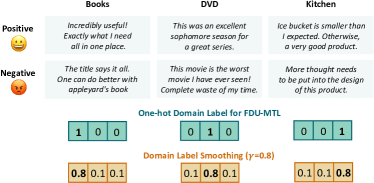
Figure 2: An example of DLS with three domains on the FDU-MTL dataset.

While Adversarial Training (AT) has been empirically validated for its effectiveness in minimizing domain divergence and capturing domain-invariant features Ganin et al. (2016); Chen and Cardie (2018), it is widely recognized that AT models can be challenging to train and may struggle to converge Roth et al. (2017); Jenni and Favaro (2019); Arjovsky and Bottou (2017). This challenge primarily stems from the utilization of one-hot domain labels, which tends to lead to highly over-confident output probabilities. This over-confidence in the domain discriminator can generate substantial oscillatory gradients, adversely affecting the stability of the training process Arjovsky and Bottou (2017); Mescheder et al. (2018). To address the challenge of overconfidence in domain predictions, our model incorporates a technique referred to as Domain Label Smoothing (DLS), as depicted in Figure 2. This approach is designed to temper the domain discriminator’s predictions, shifting from absolute and potentially overconfident classifications to the estimation of softer, more nuanced probabilities Zhang et al. (2023). The DLS formulation is as follows:

$$\mathcal{J}_{D}^{els}(F_{s},D)= \sum_{i=1}^{M}\mathbb{E}_{\textbf{x}\sim\mathbb{L}_{i}\cup\mathbb{U}_{i}}[\gamma\log(\mathcal{D}_{i}(F_{s}(\textbf{x})))$$

$$+\frac{1-\gamma}{M-1}\sum_{j=1,j\neq i}^{M}\log(\mathcal{D}_{j}(F_{s}(\textbf{x})))],$$ (5)

Where $\mathcal{D}_{i}$ gives the $i$-th dimension of the domain discriminator’s output vector and $\gamma$ ($\gamma\in(0,1)$) is a hyperparameter. DLS is both theoretically and empirically proven to bolster the model’s robustness against noisy domain labels and accelerate convergence. It promotes stable training and superior generalization performance, all without necessitating extra parameters or additional optimization steps.

With Eq.4 and Eq.3.3, the adversarial training can be updated as:

$$\min\limits_{F_{s},F_{d},C}\max\limits_{D}\mathcal{J}_{C}(F_{s},F_{d},C)+\lambda\mathcal{J}_{D}^{els}(F_{s},D)$$ (6)

3.4 Enhancement via robust pseudo-label regularization

The abundance of unlabeled data in each domain presents an opportunity to utilize pseudo-labels to refine feature discriminability in MDTC task. However, not all unlabeled data contribute positively. To judiciously select the unlabeled data that can yield dependable pseudo-labels, we incorporate the Robust Pseudo Label Regularization (RPLR) technique into our proposed SAN framework Gu et al. (2020). RPLR operates by evaluating the reliability of pseudo-labels for unlabeled data, gauging this based on the feature distance to the corresponding class center within a spherical feature space. It identifies incorrectly labeled data as outliers and employs a Gaussian-uniform mixture model to characterize the conditional probability of a data point being an outlier or an inlier. For an input instance $\textbf{x}^{u}_{j}$ its generated pseudo-label $\hat{y}^{u}_{j}$ is defined as: $\hat{y}^{u}_{j}=\arg\max\limits_{k}[C[F_{s}(\textbf{x}^{u}_{j}),F_{d}(\textbf{x}^{u}_{j})]]_{k}$, where $[\cdot]_{k}$ denotes the $k$-th element. To assess the accuracy of the generated pseudo-label, we introduce a binary random variable $z_{j}\in\{0,1\}$, indicating the correctness of the labeling with 1 for correct and 0 for incorrect. RPLR is then articulated as follows:

$$\mathcal{J}_{C}^{rplr} (F_{s},F_{d},C,\phi)=$$

$$\sum_{i=1}^{M}\mathbb{E}_{\textbf{x}^{u}_{j}\sim\mathbb{U}_{i}}[w(\textbf{x}^{u}_{j})\mathcal{L}(C[F_{s}(\textbf{x}^{u}_{j}),F_{d}(\textbf{x}^{u}_{j})],\hat{y}^{u}_{j})]$$ (7)

$$w(\textbf{x}^{u}_{j})=\begin{cases}\beta_{j}&\text{ if }\beta_{j}>0.5\\ 0&\text{ otherwise }\end{cases}$$ (8)

Where $\beta_{j}$ represents the probability of correctly labeled data, i.e., $\beta=Pr(z_{j}=1|\textbf{x}^{u}_{j},\hat{y}^{u}_{j})$. In this manner, unlabeled data with a probability of correct labeling below 0.5 are discarded. The posterior probability of correct labeling, i.e., $Pr(z=1|\textbf{x}_{j},\hat{y}_{j}),$ is modeled by the feature distance between the data and the class center to which it belongs, using a Gaussian-uniform mixture model based on pseudo-labels. Given a feature vector $f^{u}_{j}=[F_{s}(\textbf{x}^{u}_{j}),F_{d}(\textbf{x}^{u}_{j})]$ of an unlabeled instance $\textbf{x}^{u}_{j}$, its distance to the corresponding class center $\mathcal{C}_{\hat{y}^{u}_{j}}$ for category $\hat{y}^{u}_{j}$ is calculated as:

$$d^{u}_{j}=\frac{f^{u}_{j}\cdot\mathcal{C}_{\hat{y}^{u}_{j}}}{\left\|f^{u}_{j}\right\|\left\|\mathcal{C}_{\hat{y}^{u}_{j}}\right\|}$$ (9)

The class center $\mathcal{C}_{\hat{y}^{u}_{j}}$ is defined in a spherical space as presented in Gu et al. (2020), the details of computing $\mathcal{C}_{\hat{y}^{u}_{j}}$ are available in the Appendix. The distribution of feature distance $d^{u}_{j}$ is modeled by the Gaussian-uniform mixture model, a statistical distribution considering outliers Coretto and Hennig (2016); Lathuilière et al. (2018).

$$p(d^{u}_{j}|\hat{y}^{u}_{j})=\pi_{\hat{y}^{u}_{j}}\mathcal{N}^{+}(d^{u}_{j}|0,\sigma_{\hat{y}^{u}_{j}})+(1-\pi_{\hat{y}^{u}_{j}})\mathcal{U}(0,\delta_{\hat{y}^{u}_{j}})$$ (10)

Where $\mathcal{N}^{+}(d^{u}_{j}|0,\sigma)$ denotes a density function that is proportional to Gaussian distribution when $d^{u}_{j}\geq 0$, otherwise the density is zero. $\mathcal{U}(0,\delta_{\hat{y}^{u}_{j}})$ is uniform distribution defined on $[0,\delta_{\hat{y}^{u}_{j}}]$. Specifically, the Gaussian component captures the underlying probability distribution of correctly labeled data, while the uniform component provides a robust representation of the distribution for incorrectly labeled data. With Eq.10, the posterior probability of correct labeling for unlabeled data $\textbf{x}_{j}$ is defined:

$$\beta_{j}=\frac{\pi_{\hat{y}^{u}_{j}}\mathcal{N}^{+}(d^{u}_{j}|0,\sigma_{\hat{y}^{u}_{j}})}{p(d^{u}_{j}|\hat{y}^{u}_{j})}$$ (11)

The parameters of Gaussian-uniform mixture models are $\phi=\{\pi_{k},\sigma_{k},\delta_{k}\}_{k=1}^{K}$ where $K$ is the number of classes. The details of approximating these parameters will be given in Sec. 3.5.

In summary, the ultimate optimization objective is defined as:

$$\min\limits_{F_{s},F_{d},C}\max\limits_{D}\mathcal{J}_{C}(F_{s},F_{d},C)+\lambda\mathcal{J}_{D}^{els}(F_{s},D)$$

$$+\lambda_{rplr}\mathcal{J}_{C}^{rplr}(F_{s},F_{d},C,\phi)$$ (12)

3.5 Training procedure

In this section, we present how to optimize each component in the SAN model and estimate the parameters $\phi$ of Gaussian-uniform mixture models. To optimize the ultimate object in Eq.3.4, we alternatively optimize the networks and estimate parameters $\phi$ by fixing other components following Gu et al. (2020). We first initialize $F_{s}$, $F_{d}$, $C$, $D$ with Eq.6 via training strategies as in Chen and Cardie (2018), then we take the following two steps to make the optimization.

(1) Estimating $\phi$ with fixed $F_{s}$, $F_{d}$, $C$, $D$. Fixing the parameters of $F_{s}$, $F_{d}$, $C$, $D$, we generate the pseudo-label $\hat{y}^{u}_{j}$ and calculate the distance $d^{u}_{j}$ for all unlabeled data, then $\phi$ is estimated using EM algorithm as below. Let $\tilde{d}^{u}_{j}=(-1)^{m}_{j}d^{u}_{j}$, where $m_{j}$ is sampled from Bernoulli distribution $B(1,0.5)$, and $N^{u}$ denotes the number of unlabeled data, then $\phi$ can be estimated as follows:

$$\beta^{l+1}_{j}=\frac{\pi^{l}_{\hat{y}^{u}_{j}}\mathcal{N}(\tilde{d}^{u}_{j}|0,\sigma^{l}_{\hat{y}^{u}_{l}})}{\pi^{l}_{\hat{y}^{u}_{j}}\mathcal{N}(\tilde{d}^{u}_{j}|0,\sigma^{l}_{\hat{y}^{u}_{j}})+(1-\pi^{l}_{\hat{y}^{u}_{j}})\mathcal{U}(-\delta^{l}_{\hat{y}^{u}_{j}},\delta^{l}_{\hat{y}^{u}_{j}})}$$

$$\pi^{l+1}_{k}=\frac{1}{\sum_{j=1}^{N^{u}}I_{\{\hat{y}^{u}_{j}=k\}}}\sum_{j=1}^{N^{u}}I_{\{\hat{y}^{u}_{j}=k\}}\beta_{j}^{l+1}$$

$$\sigma_{j}^{l+1}=\frac{\sum_{j=1}^{N^{u}}I_{\{\hat{y}^{u}_{j}=k\}}\beta_{j}^{l+1}(\tilde{d}^{u}_{j})^{2}}{\sum_{j=1}^{N^{u}}I_{\{\hat{y}^{u}_{j}=k\}}\beta_{j}^{l+1}},\delta_{k}^{l+1}=\sqrt{3(q_{2}-q_{1}^{2})}$$

Where

$$q_{1}=\frac{1}{\sum_{j=1}^{N^{u}}I_{\{\hat{y}^{u}_{j}=k\}}\beta_{j}^{l+1}}\sum_{j=1}^{N^{u}}\frac{1-\beta_{j}^{l+1}}{1-\pi_{k}^{l+1}}I_{\{\hat{y}^{u}_{j}=k\}}\tilde{d}^{u}_{j}$$

$$q_{2}=\frac{1}{\sum_{j=1}^{N^{u}}I_{\{\hat{y}^{u}_{j}=k\}}\beta_{j}^{l+1}}\sum_{j=1}^{N^{u}}\frac{1-\beta_{j}^{l+1}}{1-\pi_{k}^{l+1}}I_{\{\hat{y}^{u}_{j}=k\}}(\tilde{d}^{u}_{j})^{2}$$

We refer our readers to Gu et al. (2020) for the deduction details of the parameters $\phi$.

(2) Optimizing $F_{s}$, $F_{d}$, $C$, $D$ with fixed $\phi$. Given current pseudo-labels and estimated $\phi$, we follow the standard MDTC training protocol Chen and Cardie (2018) to train $F_{s}$, $F_{d}$, $C$, $D$ with Eq.3.4.

4 Experiments

Domain	CMSC-LS	CMSC-SVM	CMSC-Log	MAN-L2	MAN-NLL	CAN	CRAL	SAN(Ours)
books	82.10	82.26	81.81	82.46	82.98	83.76	85.26	$\mathbf{86.29\pm 0.26}$
DVD	82.40	83.48	83.73	83.98	84.03	84.68	85.83	$\mathbf{86.43\pm 0.38}$
electronics	86.12	86.76	86.67	87.22	87.06	88.34	89.32	$\mathbf{89.78\pm 0.12}$
kitchen	87.56	88.20	88.23	88.53	88.57	90.03	$\mathbf{91.60}$	91.31$\pm 0.15$
AVG	84.55	85.18	85.11	85.55	85.66	86.70	88.00	$\mathbf{88.45\pm 0.08}$

Table 1: MDTC results on the Amazon review dataset.

Domain	MT-CNN	MT-DNN	ASP-MTL	BERT	MAN-L2	MAN-NLL	DA-MTL	GLR-MTL	SAN(Ours)
books	84.5	82.2	84.0	87.0	87.6	86.8	88.5	88.3	$\mathbf{90.5\pm 0.3}$
electronics	83.2	88.3	86.8	88.3	87.4	88.8	89.0	$\mathbf{90.3}$	87.7$\pm$0.6
dvd	84.0	84.2	85.5	85.6	88.1	88.6	88.0	87.3	$\mathbf{89.7\pm 0.5}$
kitchen	83.2	80.7	86.2	$\mathbf{91.0}$	89.8	89.9	89.0	89.8	90.4$\pm$0.9
apparel	83.7	85.0	87.0	$\mathbf{90.0}$	87.6	87.6	88.8	88.2	87.4$\pm$0.7
camera	86.0	86.2	89.2	90.0	$\mathbf{91.4}$	90.7	91.8	89.5	91.1$\pm$0.6
health	87.2	85.7	88.2	88.3	89.8	89.4	90.3	$\mathbf{90.5}$	90.3$\pm$0.3
music	83.7	84.7	82.5	86.8	85.9	85.5	85.0	$\mathbf{87.5}$	85.9$\pm$0.8
toys	89.2	87.7	88.0	91.3	90.0	$\mathbf{90.4}$	89.5	89.8	90.3$\pm$0.7
video	81.5	85.0	84.5	88.0	89.5	89.6	89.5	$\mathbf{90.8}$	90.0$\pm$0.5
baby	87.7	88.0	88.2	91.5	90.0	90.2	90.5	$\mathbf{92.3}$	90.7$\pm$0.8
magazine	87.7	89.5	92.2	$\mathbf{92.8}$	92.5	92.9	92.0	92.3	92.3$\pm$0.1
software	86.5	85.7	87.2	89.3	90.4	90.9	90.8	$\mathbf{91.8}$	89.5$\pm$0.4
sports	84.0	83.2	85.7	90.8	89.0	89.0	$\mathbf{89.8}$	87.8	$\mathbf{90.0\pm 0.2}$
IMDb	86.2	83.2	85.5	85.8	86.6	87.0	89.8	87.5	89.3$\pm 0.7$
MR	74.5	75.5	$\mathbf{76.7}$	74.0	76.1	76.7	75.5	72.7	76.5$\pm 0.9$
AVG	84.5	84.3	86.1	88.1	88.2	88.4	88.2	88.5	$\mathbf{88.8\pm 0.1}$

Table 2: MDTC results on the FDU-MTL dataset.

This section will expand on the three aspects of experiments setup, experiments results, and efficiency analysis.

4.1 Setup

Datasets. We conducted experiments on two benchmark datasets for MDTC task: the Amazon review dataset Blitzer et al. (2007) and the FDU-MTL dataset Liu et al. (2017). The Amazon review dataset comprises four domains: books, DVDs, electronics, and kitchen. Each domain consists of 2000 labeled data instances, with 1000 positive and 1000 negative examples. The data has been pre-processed into a bag-of-features representation, which includes unigrams and bigrams, without preserving word order information. The FDU-MTL dataset reflects real-world scenarios, as it contains raw text data. It encompasses 14 product review domains, including books, electronics, DVDs, kitchen, apparel, camera, health, music, toys, video, baby, magazine, software, sport, as well as two movie review domains: IMDB and MR. Each domain includes a validation set of 200 samples and a test set of 400 samples. The number of samples in the training and unlabeled sets varies across domains, but generally consists of approximately 1400 and 2000 instances, respectively.

Domain	mSDA	DANN	MDAN(H)	MDAN(S)	MAN-L2	MAN-NLL	CAN	CRAL	SAN(Ours)
books	76.98	77.89	78.45	78.63	78.45	77.78	78.91	$\mathbf{82.49}$	81.48
DVD	78.61	78.86	77.97	80.65	81.57	82.74	83.37	84.30	$\mathbf{85.53}$
electronics	81.98	84.91	84.83	85.34	83.37	83.75	84.76	86.82	$\mathbf{87.12}$
kitchen	84.26	86.39	85.80	86.26	85.57	86.41	86.75	$\mathbf{89.08}$	89.00
AVG	80.46	82.01	81.76	82.72	82.24	82.67	83.45	85.67	$\mathbf{85.78}$

Table 3: Multi-source unsupervised domain adaptation results on the Amazon review dataset.

Implementation details. To ensure a fair comparison, we adopt almost identical network architectures as presented in Chen and Cardie (2018). It’s pertinent to highlight that the sole modification we introduce is the substitution of the last fully connected layer of the original domain-specific feature extractor with a stochastic layer. For the Amazon review dataset, we select the 5000 most frequent features and represent each review as a 5000-dimensional vector, where the feature values represent raw counts. Our feature extractors employ multi-layer perceptrons (MLPs) with an input size of 5000. Each feature extractor consists of two hidden layers with sizes of 1000 and 500, respectively. In the case of the FDU-MTL dataset, we employ a single-layer convolutional neural network (CNN) as the feature extractor. The CNN utilizes different kernel sizes (3, 4, 5) with a total of 200 kernels. The input to the CNN is a 100-dimensional embedding obtained by processing each word of the input sequence using word2vec Mikolov et al. (2013). For all experiments, we set the batch size to 8, the dropout rate for each component to 0.4, and the learning rate of the Adam optimizer Kingma and Ba (2014) to 0.0001. The size of the shared features is set to 128, and the size of the domain-specific features is set to 64. Both the classifier and discriminator are MLPs with hidden layer sizes matching their respective inputs (128+64 for the classifier and 128 for the domain discriminator). Furthermore, we set the hyperparameters $\lambda$ to 0.0001, $\gamma$ to 0.9, and $\lambda_{rplr}$ to 1.

Comparison methods. In the MDTC tasks, we evaluate the our SAN method against several state-of-the-art methods: The multi-task convolutional neural network (MT-CNN) Collobert and Weston (2008), the muti-task deep neural network (MT-DNN) Liu et al. (2015), the collaborative multi-domain sentiment classification method (CMSC) trained with the least square loss (CMSC-LS), the hinge loss (CMSC-SVM), the log loss (CMSC-Log) Wu and Huang (2015), the pre-trained BERT-base model fine-tuned on each domain (BERT) Devlin et al. (2018), the adversarial multi-task learning for text classification method (ASP-MTL) Liu et al. (2017), the multinomial adversarial network (MAN) trained with the least square loss (MAN-L2) and the negative log-likelihood loss (MAN-NLL) Chen and Cardie (2018), the dynamic attentive sentence encoding method (DA-MTL) Zheng et al. (2018), the global and local shared representation-based dual-channel multi-task learning method (GLR-MTL) Su et al. (2020), the conditional adversarial network (CAN) Wu et al. (2021a), and the co-regularized adversarial learning method Wu et al. (2022a). For MS-UDA experiments, the baselines involve the marginalized denoising autoencoder (mSDA) Chen et al. (2012), the domain adversarial neural network Ganin et al. (2016), the multi-source domain adaptation network (MDAN) Zhao et al. (2017), the MAN (MAN-L2 and MAN-NLL) Chen and Cardie (2018), the CAN Wu et al. (2021a) and CRAL Wu et al. (2022a).

4.2 Result

Multi-Domain Text Classification. The experimental results on the Amazon review dataset and FDU-MTL dataset are reported in Table 1 and Table 2, respectively. We report the classification results of mean $\pm$ variance over five random runs. From Table 1, it can be noted that the SAN method obtains the best classification accuracy on 3 out of 4 domains, and yield state-of-the-art results for the average classification accuracy. For the experimental results on FDU-MTL, shown in Table 2, the proposed SAN method outperforms MT-CNN and MT-DNN consistently across all domains with notable large performance gains. When compared with the state-of-the-art MAN-L2, MAN-NLL, DA-MTL, and GLR-MTL, SAN achieves competitive results in terms of average classification accuracy. The experimental results on both benchmarks validate the efficacy of our proposed method.

Multi-Source Unsupervised Domain Adaptation. In real application scenarios, it is not uncommon for the target domain to lack annotated data. Evaluating MDTC models under such circumstances is of utmost significance. In the multi-source unsupervised domain adaptation (MS-UDA) setting, we have multiple source domains, each containing both labeled and unlabeled data, and a target domain with only unlabeled data. Our MS-UDA experiments are conducted on the Amazon review dataset, following the same protocol as outlined in Chen and Cardie (2018). Specifically, in each experiment, three out of four domains were treated as source domains, while the remaining domain was treated as the target domain. As shown in Table 3, the proposed SAN method outperforms other baselines on two out of four domains as well as the average accuracy. It reveals that our SAN method has a good capacity for transferring knowledge to unseen domains. Further experimental results, including parameter sensitivity analysis, ablation study and convergence speed analysis can be found in the Appendix.

4.3 Efficiency analysis

To demonstrate the efficiency of our SAN model, this section provides a comparative analysis concentrating on two critical metrics: the number of model parameters and the running time. We compare traditional MDTC methods, notably exemplified by MAN Chen and Cardie (2018) and based on the shared-private paradigm, with our SAN approach.

Model parameter comparison. We quantify the parameter counts for the shared feature extractor $F_{s}$, domain-specific feature extractors $\{F_{d}^{i}\}_{i=1}^{M}$, classifier $C$, and domain discriminator $D$ within both our SAN model and the traditional MAN model. The results, presented in Table 4, illuminate a significant distinction: while the domain-specific feature extractors substantially contribute to the overall parameter count in traditional MDTC models, our SAN markedly reduces the parameter load attributed to these extractors.

Dataset	Amazon		FDU-MTL
Model	MAN	SAN(ours)	MAN	SAN(ours)
# Para. of $F_{s}$	5.57M	5.57M	20.20M	20.20M
# Para. of $\{F_{d}^{i}\}_{i=1}^{M}$	22.13M	5.57M	322.65M	20.20M
# Para. of $C$	0.04M	0.04M	0.04M	0.04M
# Para. of $D$	0.02M	0.02M	0.02M	0.02M
# Total Para.	27.76M	12.00M	342.91M	40.46M

Table 4: Model parameter comparison between MAN and SAN (Ours)

Model runtime comparison. We also compared the runtime of our SAN model and MAN on the Amazon review and FDU-MTL datasets, using the average training time per epoch as the indicator. The results, which are summarized in Table 5, are as follows: it is easy to observe that SAN requires less time, saving nearly 10% compared to MAN on the Amazon dataset and nearly 15% compared to MAN on the FDU-MTL dataset. This further validates the effectiveness of our SAN approach.

Model	Amazon	FDU-MTL
MAN	7.07s	70.88s
SAN(ours)	6.39s	60.72s

Table 5: Model runtime comparison between MAN and SAN (ours)

5 Conclusion

In this study, we introduce a Stochastic Adversarial Network (SAN) specifically devised for MDTC tasks. Our approach distinctively models the weights of domain-specific feature extractors through a multivariate Gaussian distribution $\mathcal{N}(\mu,\Sigma)$. This design allows for network weights to be sampled directly from the distribution when employing domain-specific feature extractors. A notable advantage of this methodology is its capacity to minimize the model’s parameter count, preventing parameter escalation with the addition of new domains. Additionally, we incorporate domain label smoothing and robust pseudo-label regularization to ensure stable adversarial training and to enhance feature discrimination. Our experimental evaluation, conducted on two MDTC benchmarks, validates the SAN model’s capability to improve system performance and demonstrates its robust generalization to unfamiliar domains.

Appendix A Center of samples on sphere

This section computes the class center of spherical samples used for robust pseudo-label regularization. Before computing the class centers on sphere, we begin by normalizing the concatenations of the shared features and domain-specific features. Let $f(\textbf{x})=[F_{s}(\textbf{x}),F_{d}(\textbf{x})]$, where $[\cdot,\cdot]$ represents the concatenation of two vectors. We then normalize features with $f^{\prime}=r\frac{f(\textbf{x})}{f(\textbf{x})}$ to obtain features in the spherical space $\mathbb{S}_{r}^{n-1}=\{f^{\prime}\in\mathbb{R}^{n}:||f^{\prime}||=r\}$. Let $f^{\prime}_{1},f^{\prime}_{2},\cdots,f^{\prime}_{m}$ be samples on the sphere $\mathbb{S}_{r}^{n-1}$, the center $\mathcal{C}$ of the samples on the sphere corresponds to the point closest to all samples, i.e., the solution of the following optimization problem:

$$\min\limits_{f^{\prime}\in\mathbb{S}_{r}^{n-1}}\frac{1}{m}\sum_{i=1}^{m}dist(f^{\prime},f^{\prime}_{i})$$ (13)

Where $dist(u,v)=1-\frac{u^{T}v}{||u||||v||}$ is the cosine distance. Since $||f^{\prime}||=r,\forall f^{\prime}\in\mathbb{S}_{r}^{n-1}$, Eq. 13 can be rewritten as:

$$\max\limits_{f^{\prime}}f^{\prime T}(\sum_{i=1}^{m}f^{\prime}_{i})\hskip 28.45274pts.t.||f^{\prime}||=r.$$ (14)

With the method of Lagrange multipliers, the center can be obtained by:

$$\mathcal{C}=\frac{r}{||\tilde{f^{\prime}}||}\tilde{f^{\prime}}$$ (15)

Where $\tilde{f^{\prime}}=\sum_{i=1}^{m}f^{\prime}_{i}$.

Appendix B How stochastic feature extractor works

The variance of the distribution, denoted as $\Sigma$, plays a crucial role in the operational dynamics of the stochastic feature extractor. As illustrated in Figure 3, the initial values of $\Sigma$ are distributed uniformly, manifesting no discernible structure. However, post-training, these values start to display more defined patterns in Figure 4 . It’s particularly noteworthy that the distribution of the domain-specific feature extractors tends to show larger variances for different domains. As the SAN model progresses towards convergence, these pronounced variances act as a mechanism to guarantee the extraction and preservation of distinct, domain-unique features across the various domains, reinforcing the model’s ability to handle domain-specific nuances effectively.

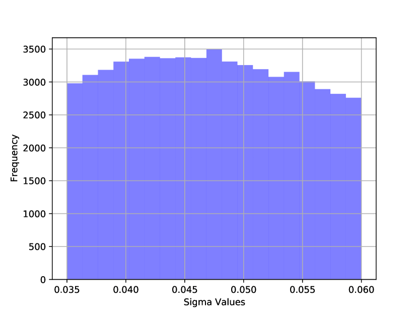
Figure 3: The distribution of the flattened $\Sigma$ values for initialization on the Amazon Review dataset.

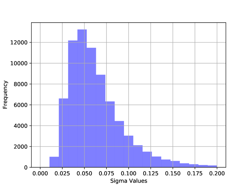
Figure 4: The distribution of the flattened $\Sigma$ values after convergence of SAN on the Amazon Review dataset.

Appendix C Experiments

C.1 Dataset

The experiments are conducted on two benchmark datasets: the Amazon review dataset Blitzer et al. [2007] and the FDU-MTL dataset Liu et al. [2017]. The statistical specifics of these datasets, which are instrumental for our analysis, are concisely presented in Table 6 for the Amazon review dataset and Table 7 for the FDU-MTL dataset.

Domain	Labeled	Unlabeled	Class.
Books	2000	4465	2
DVD	2000	5681	2
Electronics	2000	3586	2
Kitchen	2000	5945	2

Table 6: Details of the Amazon review dataset

Domain	Train	Dev.	Test	Unlabeled	Avg. L	Vocab.	Class.
Books	1400	200	400	2000	159	62K	2
Electronics	1398	200	400	2000	101	30K	2
DVD	1400	200	400	2000	173	69K	2
Kitchen	1400	200	400	2000	89	28K	2
Apparel	1400	200	400	2000	57	21K	2
Camera	1397	200	400	2000	130	26K	2
Health	1400	200	400	2000	81	26K	2
Music	1400	200	400	2000	136	60K	2
Toys	1400	200	400	2000	90	28K	2
Video	1400	200	400	2000	156	57K	2
Baby	1300	200	400	2000	104	26K	2
Magazine	1370	200	400	2000	117	30K	2
Software	1315	200	400	475	129	26K	2
Sports	1400	200	400	2000	94	30K	2
IMDB	1400	200	400	2000	269	44K	2
MR	1400	200	400	2000	21	12K	2

Table 7: Details of the FDU-MTL dataset

C.2 Validity verification of stochastic feature extractor

Method	Books	DVD	Elec.	Kit.	AVG
pSAN	82.25	83.05	86.90	88.25	85.11
pSAN w/ $F_{d}^{zero}$	81.70	82.15	86.10	87.90	84.46
pSAN w/ $F_{d}^{shuf}$	81.10	82.00	85.90	87.35	84.09

Table 8: Validity verification of stochastic feature extractor on the Amazon review dataset

We meticulously designed a suite of experiments leveraging the Amazon review dataset to empirically validate the capability of the SAN model to adeptly learn domain-specific features from multiple domains. We rigorously evaluate three variants of the model: (1) pSAN: Represents the foundational SAN model without any modifications. (2) pSAN w/ $F_{d}^{zero}$: A variant in which domain-specific features are intentionally set to zero, thereby exclusively relying on shared features for classification. (3) pSAN w/ $F_{d}^{shuf}$: This variant introduces a permutation in the domain-specific features across different domains, thereby simulating the scenario where domain-specific features from one domain are input into another. The empirical results clearly indicate that pSAN w/ $F_{d}^{shuf}$ not only lags behind the baseline pSAN but also performs inferiorly compared to pSAN w/ $F_{d}^{zero}$. This phenomenon distinctly suggests that arbitrarily shuffled domain-specific features do not contribute constructively to the classification task. Instead, they act as confounding variables, detracting from the model’s overall efficacy. This observation underscores the SAN model’s intrinsic ability to extract and leverage salient domain-specific features effectively.

C.3 Parameter sensitivity analysis

In this section, we examine the sensitivity of our SAN method to the values of hyperparameters $\lambda$, $\gamma$ and $\lambda_{rplr}$. The $\lambda$ and $\lambda_{rplr}$ are evaluated in the range $\left\{0.0001,0.05,0.1,0.5,1,10\right\}$ and $\left\{0.00001,0.0001,0.001,0.01,0.1,1\right\}$, respectively. The valid range of values for $\gamma$ is $\left(0,1\right]$, therefore we assess its impacts in the range of $\left\{0.5,0.6,0.7,0.8,0.9,0.95\right\}$. This comprehensive parameter sensitivity analysis is conducted utilizing both the Amazon review dataset and the FDU-MTL dataset. We visually present the outcomes of this investigation in Figure 5, 6 and 7, respectively, focusing on the metric of average classification accuracy.

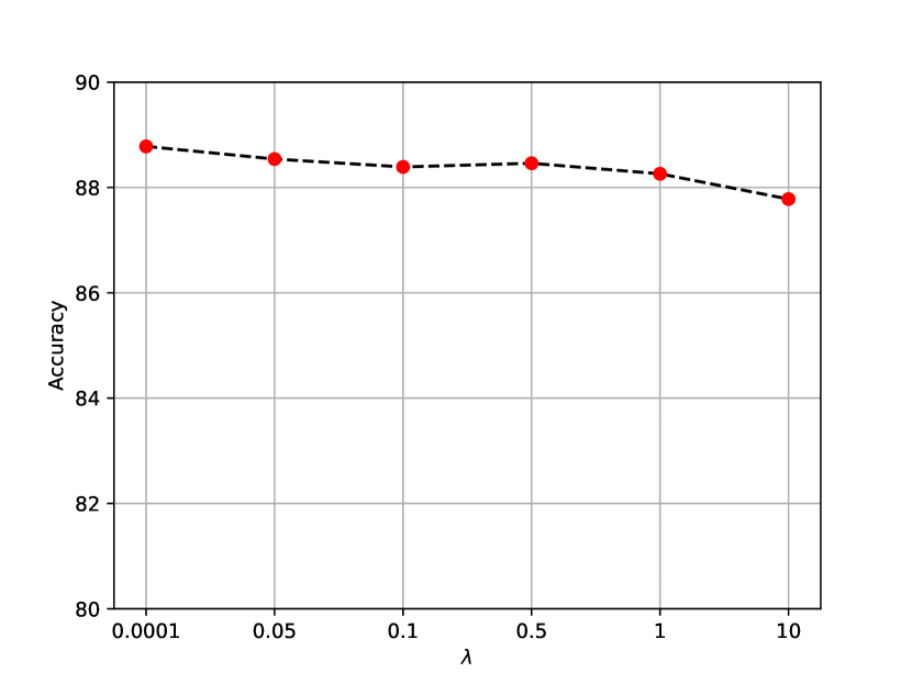
Figure 5: Parameter sensitivity analysis about $\lambda$ on Amazon review dataset.

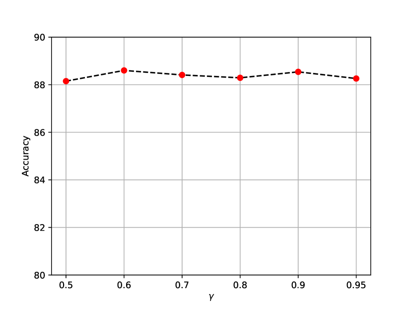
Figure 6: Parameter sensitivity analysis about $\gamma$ on Amazon review dataset.

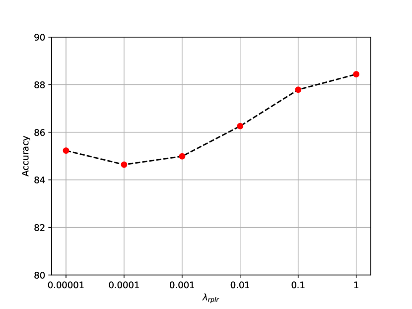
Figure 7: Parameter sensitivity analysis about $\lambda_{rplr}$ on Amazon review dataset.

C.4 Ablation study

To discern the individual impact of each constituent in our SAN methodology on the overall performance, we embark on an ablation study, leveraging both the Amazon review dataset and the FDU-MTL dataset. The outcomes of this analysis are systematically illustrated in Table 9 for the Amazon dataset and Table 10 for the FDU-MTL dataset. Specifically, we examine three variants: (1) SAN w/o dls, a variant without the enhancement of domain label smoothing; (2) SAN w/o rplr, a variant without the enhancement of robust pseudo-label regularization; (3) plain SAN, a variant utilizing a stochastic feature extractor instead of the domain-specific feature extractors of shared-private scheme. The findings from each variant underscore the integral role of the individual components, with all three variants demonstrating diminished performance compared to the comprehensive model. Notably, the full SAN model, integrating all components, consistently delivers the most superior performance, conclusively affirming the collective contribution of both domain label smoothing and robust pseudo-label regularization to the enhancement of our model’s performance.

Domain	SAN(full)	SAN w/o dls	SAN w/o rplr	plain SAN
Books	86.29	84.70	83.05	82.25
DVD	86.43	85.10	83.35	83.05
Electr.	89.78	89.75	87.75	86.90
Kit.	91.31	90.85	88.15	88.25
AVG	88.45	87.60	85.53	85.11

Table 9: Ablation study analysis on the Amazon review dataset

Domain	SAN(full)	SAN w/o dls	SAN w/o rplr	plain SAN
books	90.5	89.0	87.0	87.8
electronics	87.7	86.5	88.5	88.8
dvd	89.7	90.0	90.8	88.3
kitchen	90.4	90.3	90.5	89.8
apparel	87.4	86.0	87.5	87.3
camera	91.1	90.8	91.3	89.8
health	90.3	90.5	90.0	91.3
music	85.9	86.5	85.3	85.8
toys	90.3	91.3	90.8	89.5
video	90.0	90.3	88.3	89.5
baby	90.7	90.8	90.0	90.0
magazine	92.3	91.8	93.0	92.3
software	89.5	89.0	90.5	89.0
sports	90.0	88.0	88.8	90.3
IMDb	89.3	89.8	88.8	86.5
MR	76.5	76.3	74.3	72.0
AVG	88.8	88.5	88.4	88.0

Table 10: Ablation Study on the FDU-MTL dataset

C.5 Convergence analysis

We conducted a comparative analysis of the convergence speed between our novel SAN model and conventional MDTC methods that utilize the shared-private framework, exemplified by the Multinomial Adversarial Networks (MAN) as referenced in Chen and Cardie [2018]. The comparative results, as delineated in Figure 8, underscore the superior convergence rate of our SAN approach relative to MAN. This enhanced convergence efficiency can be attributed to the innovative implementation of the stochastic feature extractor in our SAN model, which not only streamlines the model’s learning process but also expedites its rate of convergence.

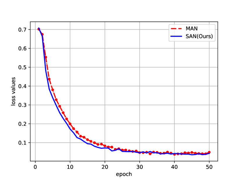
Figure 8: Convergence analysis between MAN and SAN(ours).

Method	CAN	MRAN	CRAL	MBF	RCA	SAN(ours)
Amazon	87.70	87.64	88.00	87.71	86.88	88.45
FDU-MTL	89.4	89.0	90.2	90.1	89.0	88.8

Table 11: Comparisons of SAN with several state-of-the-art methods

Domain	Books	DVD	Elec.	Kit.	AVG
Acc.	90.27	88.91	94.52	94.66	$92.09\pm 2.10$

Table 12: Accuracy of valid pseudo-labels on the Amazon review dataset

Domain	Books	Elec.	DVD	Kit.	Apparel	Camera	Health	Music	Toys	Video	Baby	Magaz.	Softw.	Sports	IMDb	MR	AVG
Acc.	89.67	94.63	90.69	95.21	96.05	94.84	93.98	87.76	93.12	90.25	93.99	95.82	92.17	95.88	89.33	82.87	$92.27\pm 3.52$

Table 13: Accuracy of valid pseudo-labels on the FDU-MTL dataset

Appendix D Limitations

While our SAN model exhibits commendable performance on the Amazon review dataset, its efficacy on the FDU-MTL dataset does not match that of the leading MDTC methods. We present a comparative analysis in Table 11, comparing our SAN model with some of the most recent MDTC methodologies, including the Conditional Adversarial Network (CAN) Wu et al. [2021a], the Mixup Regularized Adversarial Network (MRAN) Wu et al. [2021b], the Co-Regularized Adversarial Network (CRAL) Wu et al. [2022a], the Robust Contrastive Alignment (RCA) Li et al. [2022], and the Maximum Batch Frobenius Norm (MBF) Wu et al. [2022b].

A significant constraint identified in our approach pertains to the less-than-optimal accuracy of the pseudo-labels employed during the robust pseudo-label regularization process. Within the framework of the SAN model, a pseudo-labeled data point $\textbf{x}^{u}_{j}$ is deemed valid if its weight $w(\textbf{x}^{u}_{j})$ surpasses 0.5. The accuracy of these valid pseudo-labels on the unlabeled data from the Amazon review dataset is detailed in Table 12. Furthermore, Table 13 delineates the accuracy of valid pseudo-labels on both the validation and test sets of the FDU-MTL dataset. A notable observation from this data is the considerable discrepancy in pseudo-label accuracy across various domains within the FDU-MTL dataset, with the ’MR’ domain notably attaining only 82.87% accuracy. This disparity in pseudo-label quality can significantly undermine the overall performance of the system. Consequently, we posit that a pivotal area for enhancing the efficacy of our SAN model lies in improving the precision of pseudo-labels assigned to the unlabeled data, a move that is anticipated to substantially elevate the model’s performance metrics.

References

- Arjovsky and Bottou [2017] Martin Arjovsky and Léon Bottou. Towards principled methods for training generative adversarial networks. arXiv preprint arXiv:1701.04862, 2017.
- Arjovsky et al. [2017] Martin Arjovsky, Soumith Chintala, and Léon Bottou. Wasserstein generative adversarial networks. In International conference on machine learning, pages 214–223. PMLR, 2017.
- Blitzer et al. [2006] John Blitzer, Ryan McDonald, and Fernando Pereira. Domain adaptation with structural correspondence learning. In Proceedings of the 2006 conference on empirical methods in natural language processing, pages 120–128, 2006.
- Blitzer et al. [2007] John Blitzer, Mark Dredze, and Fernando Pereira. Biographies, bollywood, boom-boxes and blenders: Domain adaptation for sentiment classification. In Proceedings of the 45th annual meeting of the association of computational linguistics, pages 440–447, 2007.
- Blundell et al. [2015] Charles Blundell, Julien Cornebise, Koray Kavukcuoglu, and Daan Wierstra. Weight uncertainty in neural network. In International conference on machine learning, pages 1613–1622. PMLR, 2015.
- Bousmalis et al. [2016] Konstantinos Bousmalis, George Trigeorgis, Nathan Silberman, Dilip Krishnan, and Dumitru Erhan. Domain separation networks. Advances in neural information processing systems, 29, 2016.
- Chen and Cardie [2018] Xilun Chen and Claire Cardie. Multinomial adversarial networks for multi-domain text classification. arXiv preprint arXiv:1802.05694, 2018.
- Chen et al. [2012] Minmin Chen, Zhixiang Xu, Kilian Weinberger, and Fei Sha. Marginalized denoising autoencoders for domain adaptation. arXiv preprint arXiv:1206.4683, 2012.
- Collobert and Weston [2008] Ronan Collobert and Jason Weston. A unified architecture for natural language processing: Deep neural networks with multitask learning. In Proceedings of the 25th international conference on Machine learning, pages 160–167, 2008.
- Coretto and Hennig [2016] Pietro Coretto and Christian Hennig. Robust improper maximum likelihood: tuning, computation, and a comparison with other methods for robust gaussian clustering. Journal of the American Statistical Association, 111(516):1648–1659, 2016.
- Creswell et al. [2018] Antonia Creswell, Tom White, Vincent Dumoulin, Kai Arulkumaran, Biswa Sengupta, and Anil A Bharath. Generative adversarial networks: An overview. IEEE signal processing magazine, 35(1):53–65, 2018.
- Devlin et al. [2018] Jacob Devlin, Ming-Wei Chang, Kenton Lee, and Kristina Toutanova. Bert: Pre-training of deep bidirectional transformers for language understanding. arXiv preprint arXiv:1810.04805, 2018.
- Ganin et al. [2016] Yaroslav Ganin, Evgeniya Ustinova, Hana Ajakan, Pascal Germain, Hugo Larochelle, François Laviolette, Mario March, and Victor Lempitsky. Domain-adversarial training of neural networks. Journal of machine learning research, 17(59):1–35, 2016.
- Gu et al. [2020] Xiang Gu, Jian Sun, and Zongben Xu. Spherical space domain adaptation with robust pseudo-label loss. In Proceedings of the IEEE/CVF Conference on Computer Vision and Pattern Recognition, pages 9101–9110, 2020.
- Hernández-Lobato and Adams [2015] José Miguel Hernández-Lobato and Ryan Adams. Probabilistic backpropagation for scalable learning of bayesian neural networks. In International conference on machine learning, pages 1861–1869. PMLR, 2015.
- Hu and Wu [2024] Juntao Hu and Yuan Wu. Regularized conditional alignment for multi-domain text classification. In ICASSP 2024-2024 IEEE International Conference on Acoustics, Speech and Signal Processing (ICASSP), pages 5645–5649. IEEE, 2024.
- Jenni and Favaro [2019] Simon Jenni and Paolo Favaro. On stabilizing generative adversarial training with noise. In Proceedings of the IEEE/CVF Conference on Computer Vision and Pattern Recognition, pages 12145–12153, 2019.
- Khurana et al. [2023] Diksha Khurana, Aditya Koli, Kiran Khatter, and Sukhdev Singh. Natural language processing: State of the art, current trends and challenges. Multimedia tools and applications, 82(3):3713–3744, 2023.
- Kingma and Ba [2014] Diederik P Kingma and Jimmy Ba. Adam: A method for stochastic optimization. arXiv preprint arXiv:1412.6980, 2014.
- Kingma and Welling [2013] Diederik P Kingma and Max Welling. Auto-encoding variational bayes. arXiv preprint arXiv:1312.6114, 2013.
- Kowsari et al. [2019] Kamran Kowsari, Kiana Jafari Meimandi, Mojtaba Heidarysafa, Sanjana Mendu, Laura Barnes, and Donald Brown. Text classification algorithms: A survey. Information, 10(4):150, 2019.
- Lathuilière et al. [2018] Stéphane Lathuilière, Pablo Mesejo, Xavier Alameda-Pineda, and Radu Horaud. Deepgum: Learning deep robust regression with a gaussian-uniform mixture model. In Proceedings of the European Conference on Computer Vision (ECCV), pages 202–217, 2018.
- Li and Zong [2008] Shoushan Li and Chengqing Zong. Multi-domain sentiment classification. In Proceedings of ACL-08: HLT, Short Papers, pages 257–260, 2008.
- Li et al. [2012] Lianghao Li, Xiaoming Jin, Sinno Jialin Pan, and Jian-Tao Sun. Multi-domain active learning for text classification. In Proceedings of the 18th ACM SIGKDD international conference on Knowledge discovery and data mining, pages 1086–1094, 2012.
- Li et al. [2022] Xuefeng Li, Hao Lei, Liwen Wang, Guanting Dong, Jinzheng Zhao, Jiachi Liu, Weiran Xu, and Chunyun Zhang. A robust contrastive alignment method for multi-domain text classification. In ICASSP 2022-2022 IEEE International Conference on Acoustics, Speech and Signal Processing (ICASSP), pages 7827–7831. IEEE, 2022.
- Liu et al. [2015] Xiaodong Liu, Jianfeng Gao, Xiaodong He, Li Deng, Kevin Duh, and Ye-Yi Wang. Representation learning using multi-task deep neural networks for semantic classification and information retrieval. 2015.
- Liu et al. [2017] Pengfei Liu, Xipeng Qiu, and Xuanjing Huang. Adversarial multi-task learning for text classification. arXiv preprint arXiv:1704.05742, 2017.
- Long et al. [2018] Mingsheng Long, Zhangjie Cao, Jianmin Wang, and Michael I Jordan. Conditional adversarial domain adaptation. Advances in neural information processing systems, 31, 2018.
- Lu et al. [2020] Zhihe Lu, Yongxin Yang, Xiatian Zhu, Cong Liu, Yi-Zhe Song, and Tao Xiang. Stochastic classifiers for unsupervised domain adaptation. In Proceedings of the IEEE/CVF Conference on Computer Vision and Pattern Recognition, pages 9111–9120, 2020.
- Mescheder et al. [2018] Lars Mescheder, Andreas Geiger, and Sebastian Nowozin. Which training methods for gans do actually converge? In International conference on machine learning, pages 3481–3490. PMLR, 2018.
- Mikolov et al. [2013] Tomas Mikolov, Kai Chen, Greg Corrado, and Jeffrey Dean. Efficient estimation of word representations in vector space. arXiv preprint arXiv:1301.3781, 2013.
- Roth et al. [2017] Kevin Roth, Aurelien Lucchi, Sebastian Nowozin, and Thomas Hofmann. Stabilizing training of generative adversarial networks through regularization. Advances in neural information processing systems, 30, 2017.
- Su et al. [2020] Xuefeng Su, Ru Li, and Xiaoli Li. Multi-domain transfer learning for text classification. In CCF International Conference on Natural Language Processing and Chinese Computing, pages 457–469. Springer, 2020.
- Subedar et al. [2019] Mahesh Subedar, Ranganath Krishnan, Paulo Lopez Meyer, Omesh Tickoo, and Jonathan Huang. Uncertainty-aware audiovisual activity recognition using deep bayesian variational inference. In Proceedings of the IEEE/CVF international conference on computer vision, pages 6301–6310, 2019.
- Vaswani et al. [2017] Ashish Vaswani, Noam Shazeer, Niki Parmar, Jakob Uszkoreit, Llion Jones, Aidan N Gomez, Łukasz Kaiser, and Illia Polosukhin. Attention is all you need. Advances in neural information processing systems, 30, 2017.
- Wang and Yeung [2020] Hao Wang and Dit-Yan Yeung. A survey on bayesian deep learning. ACM computing surveys (csur), 53(5):1–37, 2020.
- Wu and Guo [2020] Yuan Wu and Yuhong Guo. Dual adversarial co-learning for multi-domain text classification. In Proceedings of the AAAI conference on artificial intelligence, volume 34, pages 6438–6445, 2020.
- Wu and Huang [2015] Fangzhao Wu and Yongfeng Huang. Collaborative multi-domain sentiment classification. In 2015 IEEE international conference on data mining, pages 459–468. IEEE, 2015.
- Wu et al. [2021a] Yuan Wu, Diana Inkpen, and Ahmed El-Roby. Conditional adversarial networks for multi-domain text classification. arXiv preprint arXiv:2102.10176, 2021.
- Wu et al. [2021b] Yuan Wu, Diana Inkpen, and Ahmed El-Roby. Mixup regularized adversarial networks for multi-domain text classification. In ICASSP 2021-2021 IEEE International Conference on Acoustics, Speech and Signal Processing (ICASSP), pages 7733–7737. IEEE, 2021.
- Wu et al. [2022a] Yuan Wu, Diana Inkpen, and Ahmed El-Roby. Co-regularized adversarial learning for multi-domain text classification. In International Conference on Artificial Intelligence and Statistics, pages 6690–6701. PMLR, 2022.
- Wu et al. [2022b] Yuan Wu, Diana Inkpen, and Ahmed El-Roby. Maximum batch frobenius norm for multi-domain text classification. In ICASSP 2022-2022 IEEE International Conference on Acoustics, Speech and Signal Processing (ICASSP), pages 3763–3767. IEEE, 2022.
- Yu et al. [2019] Tianyuan Yu, Da Li, Yongxin Yang, Timothy M Hospedales, and Tao Xiang. Robust person re-identification by modelling feature uncertainty. In Proceedings of the IEEE/CVF international conference on computer vision, pages 552–561, 2019.
- Zhang et al. [2015] Xiang Zhang, Junbo Zhao, and Yann LeCun. Character-level convolutional networks for text classification. Advances in neural information processing systems, 28, 2015.
- Zhang et al. [2023] YiFan Zhang, Xue Wang, Jian Liang, Zhang Zhang, Liang Wang, Rong Jin, and Tieniu Tan. Free lunch for domain adversarial training: Environment label smoothing. arXiv preprint arXiv:2302.00194, 2023.
- Zhao et al. [2017] Han Zhao, Shanghang Zhang, Guanhang Wu, Joao P Costeira, José MF Moura, and Geoffrey J Gordon. Multiple source domain adaptation with adversarial training of neural networks. arXiv preprint arXiv:1705.09684, 2017.
- Zheng et al. [2018] Renjie Zheng, Junkun Chen, and Xipeng Qiu. Same representation, different attentions: Shareable sentence representation learning from multiple tasks. arXiv preprint arXiv:1804.08139, 2018.
- Zhou et al. [2024] Yue Zhou, Chenlu Guo, Xu Wang, Yi Chang, and Yuan Wu. A survey on data augmentation in large model era. arXiv preprint arXiv:2401.15422, 2024.