G-Transformer for Conditional Average Potential Outcome Estimation over Time

Abstract

Estimating potential outcomes for treatments over time based on observational data is important for personalized decision-making in medicine. Yet, existing neural methods for this task suffer from either (a) bias or (b) large variance. In order to address both limitations, we introduce the G-transformer (GT). Our GT is a novel, neural end-to-end model designed for unbiased, low-variance estimation of conditional average potential outcomes (CAPOs) over time. Specifically, our GT is the first neural model to perform regression-based iterative G-computation for CAPOs in the time-varying setting. We evaluate the effectiveness of our GT across various experiments. In sum, this work represents a significant step towards personalized decision-making from electronic health records.

1 Introduction

Causal machine learning has recently garnered significant attention with the aim to personalize treatment decisions in medicine [9]. Here, an important task is to estimate conditional average potential outcomes (CAPOs) from observational data over time (see Fig. 1). Recently, such data has become prominent in medicine due to the growing prevalence of electronic health records (EHRs) [2, 7] and wearable devices [5, 27].

Several neural methods have been developed for estimating CAPOs over time. However, existing methods suffer from one of two possible limitations (see Table 1):  Methods without proper causal adjustments [6, 25, 37] exhibit significant bias. Hence, these methods have irreducible estimation errors irrespective of the amount of available data, which renders them unsuitable for medical applications.  Methods that perform proper time-varying adjustments [20, 21] suffer from large variance. Here, the causal adjustments are based on the estimation of either the probability distributions of all time-varying covariates, or the propensity scores at several time steps in the future. While the former is impracticable when granular patient information is available, the latter suffers from strong overlap violations in the time-varying setting. To the best of our knowledge, there is no method that can address both and .

To fill the above research gap, we propose the G-transformer (GT), a novel, neural end-to-end transformer that overcomes both limitations of existing methods. Our GT builds upon G-computation [4, 32]. However, unlike existing neural models that perform G-computation [20], our GT is based on an iterative regression scheme and does not require estimating any probability distribution. As a result, our GT has two clear strengths:  it is unbiased through proper causal adjustments, and it has  low variance.

Our contributions are three-fold: (1) We introduce the first  unbiased,  low-variance neural end-to-end model for estimating conditional average potential outcomes (CAPOs) over time. (2) To the best of our knowledge, we are the first to leverage regression-based iterative G-computation for estimating CAPOs over time. (3) We demonstrate the effectiveness of our GT across various experiments. In the future, we expect our GT to help personalize decision-making from patient trajectories in medicine.

2 Related Work

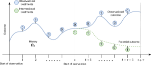
Figure 1: Trajectories with outcomes under observational vs. interventional treatment sequences.

	CRN [6]	TE-CDE [37]	CT [25]	RMSNs [21]	G-Net [20]	GT (ours)
Unbiased	✗	✗	✗	✓	✓	✓
Low variance	✓	✓	✓	✗	✗	✓

Table 1: Overview of key neural methods for estimating CAPOs over time. Unbiased methods perform proper causal adjustments. Methods with low variance only require estimation of expectations instead of full probability distributions.

Estimating CAPOs in the static setting: Extensive work on estimating potential outcomes focuses on the static setting (e.g., [1, 10, 16, 23, 26, 46, 47]). However, observational data such as electronic health records (EHRs) in clinical settings are typically measured over time [2, 7]. Hence, static methods are not tailored to accurately estimate potential outcomes when (i) time series data is observed and (ii) multiple treatments in the future are of interest.

Estimating APOs over time: Estimating average potential outcomes (APOs) over time has a long-ranging history in classical statistics and epidemiology [22, 29, 35, 41]. Popular approaches are the G-methods [32], which include marginal structural models (MSMs) [32, 33], structural nested models [30, 32] and the G-computation [4, 31, 32]. G-computation has also been incorporated into neural models [11]. However, these works do not focus estimating CAPOs. Therefore, they are not suitable for personalized decision-making.

Estimating CAPOs over time: In this work, we focus on the task of estimating the heterogeneous response to a sequence of treatments through conditional average potential outcomes (CAPOs). There are some non-parametric methods for this task [36, 40, 45], yet these suffer from poor scalability and have limited flexibility regarding the outcome distribution, the dimension of the outcomes, and static covariate data; because of that, we do not explore non-parametric methods further but focus on neural methods instead. Hence, we now summarize key neural methods that have been developed for estimating CAPOs over time (see Table 1). However, these methods fall into two groups with important limitations, as discussed in the following:

Limitation  bias: A number of neural methods for estimating CAPOs have been proposed that do not properly adjust for time-varying confounders and, therefore, are biased [6, 25, 37]. Here, key examples are the counterfactual recurrent network (CRN) [6], the treatment effect neural controlled differential equation (TE-CDE) [37] and the causal transformer (CT) [25]. These methods try to account for time-varying confounders through balanced representations. However, balancing was originally designed for reducing finite-sample estimation variance and not for mitigating confounding bias [38]. Hence, this is a heuristic and may even introduce another source of representation-induced confounding bias [24]. Unlike these methods, our GT is unbiased through proper causal adjustments.

Limitation  variance: Existing neural methods with proper causal adjustments require estimating full probability distributions at several time steps in the future, which leads to large variance. Prominent examples are the recurrent marginal structural networks (RMSNs) [21] and the G-Net [20]. Here, the RMSNs leverage MSMs [32, 33] and construct pseudo outcomes through inverse propensity weighting (IPW) in order to mimic data of a randomized control trial. However, IPW is particularly problematic in the time-varying setting due to severe overlap violations. Hence, IPW can lead to extreme weights and, therefore, large variance. Further, the G-Net [20] uses G-computation [31, 32] to adjust for confounding. G-computation is an adjustment that marginalizes over the distribution of time-varying confounders under an interventional sequence of treatments (see Supplement A). However, G-Net proceeds by estimating the entire distribution of all confounders at several time-steps in the future. Hence, when granular patient information is available, G-Net is subject to the curse of dimensionality and, therefore, also suffers from large variance. Different to these methods, our GT makes use of regression-based G-computation, which leads to low variance.

Research gap: None of the above neural methods leverages G-computation [4, 31] for estimating CAPOs through iterative regressions. Therefore, to the best of our knowledge, we propose the first neural end-to-end model that properly adjusts for time-varying confounders through regression-based iterative G-computation. Hence, our GT yields estimates of CAPOs over time that are  unbiased and have  low-variance.

3 Problem Formulation

Setup: We follow previous literature [6, 20, 21, 25] and consider data that consist of realizations of the following random variables: (i) outcomes $Y_{t}\in\mathbb{R}^{d_{y}}$, (ii) covariates $X_{t}\in\mathbb{R}^{d_{x}}$, and (iii) treatments $A_{t}\in\{0,1\}^{d_{a}}$ at time steps ${t\in\{0,\ldots,T\}\subset\mathbb{N}_{0}}$, where $T$ is the time window that follows some unknown counting process. We write ${U_{t:t+\tau}=(U_{t},\ldots,U_{t+\tau})}$ to refer to a specific subsequence of a random variable $U_{t}\in\{Y_{t},X_{t},A_{t}\}$. We further write $\bar{U}_{t}=U_{0:t}$ to denote the full trajectory of $U$ including time $t$. Finally, we write ${\bar{H}_{t+\delta}^{t}=(\bar{Y}_{t+\delta},\bar{X}_{t+\delta},\bar{A}_{t-1})}$ for $\delta\geq 0$, and we let ${\bar{H}_{t}=\bar{H}_{t}^{t}}$ denote the collective history of (i)–(iii).

Estimation task: We are interested in estimating the conditional average potential outcome (CAPO) for a future, interventional sequence of treatments, given the observed history. For this, we build upon the potential outcomes framework [28, 34] for the time-varying setting [32, 33]. Hence, we aim to estimate the potential outcome ${Y_{t+\tau}[a_{t:t+\tau-1}]}$ at future time $t+\tau$, $\tau\in\mathbb{N}$, for an interventional sequence of treatments $a=a_{t:t+\tau-1}$, conditionally on the observed history $\bar{H}_{t}=\bar{h}_{t}$. That is, our objective is to estimate

$$\mathbb{E}\left[Y_{t+\tau}[a_{t:t+\tau-1}]\mid\bar{H}_{t}=\bar{h}_{t}\right].$$ (1)

Identifiability: In order to estimate the causal quantity in Eq. (1) from observational data, we make the following identifiability assumptions [32, 33] that are standard in the literature [6, 20, 21, 25, 37]: (1) Consistency: For an observed sequence of treatments $\bar{A}_{t}=\bar{a}_{t}$, the observed outcome $Y_{t+1}$ equals the corresponding potential outcome $Y_{t+1}[\bar{a}_{t}]$. (2) Positivity: For any history $\bar{H}_{t}=\bar{h}_{t}$ that has non-zero probability $\mathbb{P}(\bar{H}_{t}=\bar{h}_{t})>0$, there is a positive probability $\mathbb{P}(A_{t}=a_{t}\mid\bar{H}_{t}=\bar{h}_{t})>0$ of receiving any treatment $A_{t}=a_{t}$, where $a_{t}\in\{0,1\}^{d_{a}}$. (3) Sequential ignorability: Given a history $\bar{H}_{t}=\bar{h}_{t}$, the treatment $A_{t}$ is independent of the potential outcome $Y_{t+1}[a_{t}]$, that is, ${A_{t}\perp Y_{t+1}[a_{t}]\mid\bar{H}_{t}=\bar{h}_{t}}$ for all $a_{t}\in\{0,1\}^{d_{a}}$.

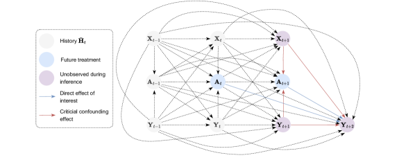
Figure 2: During inference, future time-varying confounders are unobserved. In order to estimate CAPOs for an interventional treatment sequence without bias, proper causal adjustments are required.

G-computation: Estimating CAPOs without bias poses a non-trivial challenge in the time-varying setting. The issue lies in the complexity of handling future time-varying confounders. In particular, for $\tau\geq 2$ and ${1\leq\delta\leq\delta^{\prime}\leq\tau-1}$, future covariates $X_{t+\delta}$ and outcomes $Y_{t+\delta}$ may affect the probability of receiving certain treatments $A_{t+\delta^{\prime}}$, as we illustrate in Fig. 2. Importantly, the time-varying confounders are unobserved during inference time, which is generally known as runtime confounding [8]. Therefore, in order to estimate the direct effect of an interventional treatment sequence, the time-varying confounders need to be adjusted for.

To address the above challenge, the literature suggests to marginalize over the distribution of these future confounders under the interventional sequence of treatments $a=a_{t:t+\tau-1}$. For this, we leverage G-computation [4, 31, 32], which provides a rigorous way to account for the time-varying confounders and, hence, to get unbiased estimates. Formally, G-computation identifies the causal quantity in Eq. (1) via

$$\mathbb{E}[Y_{t+\tau}[a_{t:t+\tau-1}]\mid\bar{H}_{t}=\bar{h}_{t}]$$

$$= \mathbb{E}\bigg{\{}\mathbb{E}\bigg{[}\ldots\mathbb{E}\big{\{}\mathbb{E}[Y_{t+\tau}\mid\bar{H}_{t+\tau-1}^{t},A_{t:t+\tau-1}=a_{t:t+\tau-1}]\mid\bar{H}_{t+\tau-2}^{t},A_{t:t+\tau-2}=a_{t:t+\tau-2}\big{\}}$$ (2)

$$\quad\quad\quad\ldots\bigl{\lvert}\bar{H}_{t+1}^{t},A_{t:t+1}=a_{t:t+1}\bigg{]}\bigl{\lvert}\bar{H}_{t}=\bar{h}_{t},A_{t}=a_{t}\bigg{\}}.$$

A derivation of the G-computation formula for CAPOs is given in Supplement A. However, due to the nested structure of G-computation, estimating Eq. (3) from data is challenging.

So far, only G-Net [20] has used G-computation for estimating CAPOs in a neural model. For this, G-Net makes a Monte Carlo approximation of Eq. (3) through

$$\int_{\mathbb{R}^{d_{x}\times\tau-1}\times\mathbb{R}^{d_{y}\times\tau-1}}\mathbb{E}[Y_{t+\tau}\mid\bar{H}_{t+\tau-1}^{t}=\bar{h}_{t+\tau-1}^{t},A_{t:t+\tau-1}=a_{t:t+\tau-1}]$$

$$\times\prod_{\delta=1}^{\tau-1}p(x_{t+\delta},y_{t+\delta}\mid\bar{h}_{t},{x}_{t+1:t+\delta-1},{y}_{t+1:t+\delta-1},{a}_{t:t+\delta-1})\mathop{}\!\mathrm{d}p({x}_{t+1:t+\tau-1}{y}_{t+1:t+\tau-1}).$$ (3)

However, Eq. (3) requires estimating the distribution of all time-varying confounders at several time-steps in the future, which leads to large variance.

In contrast, our GT does not rely on high-dimensional integral approximation through Monte Carlo sampling. Further, our GT does not require estimating any probability distribution. Instead, it performs regression-based iterative G-computation in an end-to-end transformer architecture. Thereby, we provide unbiased, low-variance estimates of Eq. (3).

4 G-transformer

In the following, we present our G-transformer. Inspired by [4, 31, 32] for APOs, we reframe G-computation for CAPOs over time through recursive conditional expectations. Thereby, we precisely formulate the training objective of our GT through iterative regressions. Importantly, existing approaches for estimating APOs do not estimate potential outcomes on an individual level for a given history $\bar{H}_{t}=\bar{h}_{t}$, because of which they are not sufficient for estimating CAPOs. Therefore, we proceed below by first extending regression-based iterative G-computation to account for the heterogeneous response to a treatment intervention. We then detail the architecture of our GT and provide details on the end-to-end training and inference.

4.1 Regression-based iterative G-computation for CAPOs

Our GT provides unbiased estimates of Eq. (1) by leveraging G-computation as in Eq. (3). However, we do not attempt to integrate over the estimated distribution of all time-varying confounders. Instead, one of our main novelties is that our GT performs iterative regressions in a neural end-to-end architecture. This allows us to estimate Eq. (1) with low variance.

We reframe Eq. (3) equivalently as a recursion of conditional expectations. Thereby, we can precisely formulate the iterative regression objective of our GT. For this, let

$$g_{t+\delta}^{a}(\bar{h}_{t+\delta}^{t})=\mathbb{E}[G_{t+\delta+1}^{a}\mid\bar{H}_{t+\delta}^{t}=\bar{h}_{t+\delta}^{t},A_{t:t+\delta}=a_{t:t+\delta}],$$ (4)

where

$$G_{t+\tau}^{a}=Y_{t+\tau}$$ (5)

and

$$G_{t+\delta}^{a}=g_{t+\delta}^{a}(\bar{H}_{t+\delta}^{t})$$ (6)

for $\delta=0,\ldots,\tau-1$. Then, our original objective in Eq. (1) can be rewritten as

$$g_{t}^{a}(\bar{h}_{t})=\mathbb{E}[Y_{t+\tau}[a_{t:t+\tau-1}]\mid\bar{H}_{t}=\bar{h}_{t}].$$ (7)

In order to correctly estimate Eq. (7) for a given history $\bar{H}_{t}=\bar{h}_{t}$ and an interventional treatment sequence $a=a_{t:t+\tau-1}$, estimates of all subsequent conditional expectations in Eq. (4) are required. However, this is a challenging task as the ground-truth realizations of $G_{t+\delta}^{a}$ are not available in the data. Instead, only realizations of $G_{t+\tau}^{a}$ in Eq. (5) are observed during the training. Hence, when training our GT, it generates predictions $\tilde{G}_{t+\delta}^{a}$ for $\delta=1,\ldots\tau-1$, which it then uses for learning.

Therefore, the training of our GT completes two steps in an iterative scheme: First, it runs a  generation step, where it generates predictions of Eq. (6). Then, it runs a  learning step, where it regresses the predictions for Eq. (6) and the observed $G_{t+\tau}^{a}$ in Eq. (5) on the history to update the model. Finally, the updated model is used again in the next  generation step. Thereby, our GT is designed to simultaneously  generate predictions and  learn during the training. Both steps are performed in an end-to-end architecture, ensuring that information is shared across time and data is used efficiently. We detail the training and inference of our GT in the following section.

4.2 Model architecture

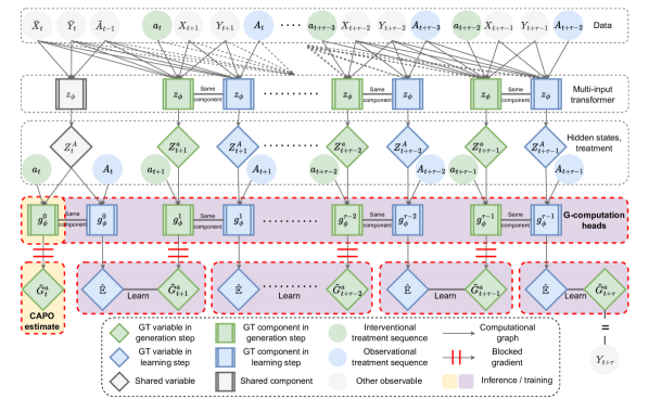
Figure 3: Neural end-to-end architecture of our G-transformer.

We first introduce the architecture of our GT. Then, we explain the iterative prediction and learning scheme inside our GT, which presents one of the main novelties. Finally, we introduce the inference procedure.

Our GT consists of two key components (see Fig. 3): (i) a multi-input transformer $z_{\phi}(\cdot)$, and (ii) several G-computation heads $\{g_{\phi}^{\delta}(\cdot)\}_{\delta=0}^{\tau-1}$, where $\phi$ denotes the trainable weights. First, the multi-input transformer encodes the entire observed history. Then, the G-computation heads take the encoded history and perform the iterative regressions according to Eq. (4). We provide further details on the transformer architecture in Supplement B. For all $t=1,\ldots,T-\tau$ and $\delta=0,\ldots,\tau-1$, the components are designed as follows:

(i) Multi-input transformer: The backbone of our GT is a multi-input transformer ${z_{\phi}(\cdot)}$, which consists of three connected encoder-only sub-transformers $z_{\phi}^{k}(\cdot)$, $k\in\{1,2,3\}$. At time $t$, the transformer $z_{\phi}(\cdot)$ receives data $\bar{H}_{t}=(\bar{Y}_{t},\bar{X}_{t},\bar{A}_{t-1})$ as input and passes them to one corresponding sub-transformer. In particular, each sub-transformer $z_{\phi}^{k}(\cdot)$ is responsible to focus on one particular $\bar{U}_{t}^{k}\in\{\bar{Y}_{t},\bar{X}_{t},\bar{A}_{t-1}\}$ in order to effectively process the different types of inputs. Further, we ensure that information is shared between the sub-transformers, as we detail below. The output of the multi-input transformer are hidden states $Z_{t}^{A}$, which are then passed to the (ii) G-computation heads.

We build upon a state-of-the-art multi-input transformer [25]. For each $\bar{U}_{t}^{k}\in\{\bar{Y}_{t},\bar{X}_{t},\bar{A}_{t-1}\}$, the sub-transformer $z_{\phi}^{k}(\cdot)$ first performs a masked multi-headed self-attention [43] on $\bar{U}_{t}^{k}$, $k\in\{1,2,3\}$, and outputs $Q_{t}^{k}$. Further, our GT builds upon masked in-between cross-attentions in order to allow the different sub-transformers to share information. For this, our GT uses $Q_{t}^{k}$ as a query to keys and values $K_{t}^{l}=V_{t}^{l}\in\{Q_{t}^{l}\mid l\in\{1,2,3\}\setminus\{k\}\}$ from both of the other two sub-transformers, respectively. Thereby, we ensure that information is shared between the each of the sub-transformers. Then, the outputs of these cross-attention mechanisms are passed through feed-forward networks and averaged. Finally, this yields a hidden state $Z_{t}^{A}$, which encodes all the information that is required for estimating the CAPO.

(ii) G-computation heads: The G-computation heads $\{g_{\phi}^{\delta}(\cdot)\}_{\delta=0}^{\tau-1}$ are the read-out component of our GT. As input at time $t+\delta$, the G-computation heads receive the hidden state $Z_{t+\delta}^{A}$ from the above multi-input-transformer. Recall that we seek to perform the iterative regressions in Eq. (4) and Eq. (7), respectively. For this, we require estimators for $\mathbb{E}[G_{t+\delta+1}^{a}\mid\bar{H}_{t+\delta},\bar{A}_{t+\delta}]$. Hence, the G-computation heads compute

$$\hat{\mathbb{E}}[G_{t+\delta+1}^{a}\mid\bar{H}_{t+\delta},{A}_{t+\delta}]=g_{\phi}^{\delta}(Z_{t+\delta}^{A},A_{t+\delta}),$$ (8)

where

$$Z_{t+\delta}^{A}=z_{\phi}(\bar{H}_{t+\delta})$$ (9)

for $\delta=0,\ldots,\tau-1$. As a result, the G-computation heads and the multi-input transformer together give the estimators that are required for the regression-based iterative G-computation. In particular, we thereby ensure that, for $\delta=0$, the last G-computation head $g_{\phi}^{0}(\cdot)$ is trained as the estimator for the CAPO as given in Eq. (7). That is, for a fully trained multi-input transformer and G-computation heads, our GT estimates the CAPO via

$$\hat{\mathbb{E}}[Y_{t+\tau}[a_{t:t+\tau-1}]\mid\bar{H}_{t}=\bar{h}_{t}]=g_{\phi}^{0}(z_{\phi}(\bar{h}_{t}),a_{t}).$$ (10)

For this, we present a tailored training procedure in the following.

4.3 Iterative training and inference time

We now introduce the iterative training of our GT, which consists of a  generation step and a  learning step. Then, we show how inference for a given history $\bar{H}_{t}=\bar{h}_{t}$ can be achieved. We provide pseudocode in Supplement C.

Iterative training: Our GT is designed to estimate the CAPO $g_{t}^{a}(\bar{h}_{t})$ in Eq. (7) for a given history $\bar{H}_{t}=\bar{h}_{t}$ and an interventional treatment sequence $a=a_{t:t+\tau-1}$. Therefore, it requires the targets $\{{G}_{t+\delta}^{a}\}_{\delta=1}^{\tau}$ in Eq. (6) during training. However, they are only available in the training data for $\delta=\tau$. As a remedy, our GT first predicts them in the  generation step. Then, it can use these generated targets for learning the network weights $\phi$ in the  learning step. In the following, we write $\tilde{G}_{t+\delta}^{a}$ for the generated targets. Note that, since ${G}_{t+\tau}^{a}=Y_{t+\tau}$ is observed during training, we do not have to generate this target. Yet, for notational convenience, we write $\tilde{G}_{t+\tau}^{a}={G}_{t+\tau}^{a}$.

 Generation step: In this step, our GT generates $\tilde{G}_{t+\delta}^{a}\approx{g}_{t+\delta}^{a}(\bar{H}_{t+\delta}^{t})$ as substitutes for Eq. (6), which are the targets in the iterative regression-based G-computation. Formally, our GT predicts these targets via

$$\tilde{G}_{t+\delta}^{a}=g_{\phi}^{\delta}(Z_{t+\delta}^{a},a_{t+\delta}),$$ (11)

where

$$Z_{t+\delta}^{a}=z_{\phi}(\bar{H}_{t+\delta}^{t},a_{t:t+\delta-1}),$$ (12)

for $\delta=0,\ldots,\tau-1$. For this, all operations are detached from the computational graph. Hence, our GT now has targets $\{\tilde{G}_{t+\delta}^{a}\}_{\delta=0}^{\tau}$, which it can use in the following  learning step.

 Learning step: This step is responsible for updating the weights $\phi$ of the multi-input transformer $z_{\phi}(\cdot)$ and the G-computation heads $\{g_{\phi}^{\delta}(\cdot)\}_{\delta=0}^{\tau-1}$. For this, our GT learns the estimator for Eq. (4) via

$$\hat{\mathbb{E}}[G_{t+\delta+1}^{a}\mid\bar{H}_{t+\delta}^{t},A_{t:t+\delta}]=g_{\phi}^{\delta}(Z_{t+\delta}^{A},A_{t+\delta}),$$ (13)

where

$$Z_{t+\delta}^{A}=z_{\phi}(\bar{H}_{t+\delta})$$ (14)

for $\delta=0,\ldots,\tau-1$. In particular, the estimator is optimized by backpropagating the squared error loss $\mathcal{L}$ for all $\delta=0,\ldots,\tau-1$ and $t=1,\ldots,T-\tau$ via

$$\mathcal{L}=\frac{1}{T-\tau}\sum_{t=1}^{T-\tau}\left(\frac{1}{\tau}\sum_{\delta=0}^{\tau-1}\left(g_{\phi}^{\delta}(Z_{t+\delta}^{A},A_{t+\delta})-\tilde{G}_{t+\delta+1}^{a}\right)^{2}\right).$$ (15)

Then, after $\phi$ is updated, we can use the updated estimator in the next  generation step.

Inference at runtime: Finally, we introduce how inference is achieved with our GT. Given a history $\bar{H}_{t}=\bar{h}_{t}$ and an interventional treatment sequence $a=a_{t:t+\tau-1}$, our GT is trained to produce an unbiased estimate of Eq. (1) through Eq. (7). For this, our GT computes the CAPO via

$$\hat{g}_{t}^{a}(\bar{h}_{t})=\hat{\mathbb{E}}[G_{t+1}^{a}\mid\bar{H}_{t}=\bar{h}_{t},A_{t}=a_{t}]=g_{\phi}^{0}(z_{\phi}(\bar{h}_{t}),a_{t}).$$ (16)

5 Experiments

We show the performance of our GT against key neural methods for estimating CAPOs over time (see Table 1). Further details (e.g., implementation details, hyperparameter tuning, runtime) are given in Supplement D.

5.1 Synthetic data

First, we follow common practice in benchmarking for causal inference [6, 15, 20, 21, 25] and evaluate the performance of our GT against other baselines on fully synthetic data. The use of synthetic data is beneficial as it allows us to simulate the outcomes under a sequence of interventions, which are unknown in real-world datasets. Thereby, we are able to evaluate the performance of all methods for estimating CAPOs over time. Here, our main aim is to show that our GT is robust against increasing levels of confounding.

Setting: For this, we use data based on the pharmacokinetic-pharmacodynamic tumor growth model [12], which is a standard dataset for benchmarking causal inference methods in the time-varying setting [6, 20, 21, 25]. Here, the outcome $Y_{t}$ is the volume of a tumor that evolves according to the stochastic process

$$Y_{t+1}=\Big{(}1+\underbrace{\rho\log\left(\tfrac{K}{Y_{t}}\right)}_{\text{Tumor growth}}-\underbrace{\alpha_{c}c_{t}}_{\text{Chemotherapy}}-\underbrace{(\alpha_{r}d_{t}+\beta_{r}d_{t}^{2})}_{\text{Radiotherapy}}+\underbrace{\epsilon_{t}}_{\text{Noise}}\Big{)}\,Y_{t},$$ (17)

where $\alpha_{c}$, $\alpha_{r}$, and $\beta_{r}$ control the strength of chemo- and radiotherapy, respectively, and where $K$ corresponds to the carrying capacity, and where $\rho$ is the growth parameter. The radiation dosage $d_{t}$ and chemotherapy drug concentration $c_{t}$ are applied with probabilities

$$A_{t}^{c},A_{t}^{r}\sim\text{Ber}\left(\sigma\left(\tfrac{\gamma}{D_{\text{{max}}}}(\bar{D}_{15}(\bar{Y}_{t-1}-\bar{D}_{\text{{max}}}/2\right)\right),$$ (18)

where $D_{\text{{max}}}$ is the maximum tumor volume, $\bar{D}_{15}$ the average tumor diameter of the last $15$ time steps, and $\gamma$ controls the confounding strength. We use the same parameterization as in [25]. For training, validation, and testing, we sample $N=1000$ trajectories of lengths $T\leq 30$ each.

$\gamma=10$ $\gamma=11$ $\gamma=12$ $\gamma=13$ $\gamma=14$ $\gamma=15$ $\gamma=16$ $\gamma=17$ $\gamma=18$ $\gamma=19$ $\gamma=20$ CRN [6] $4.05\pm 0.55$ $5.45\pm 1.68$ $6.17\pm 1.27$ $4.98\pm 1.49$ $5.24\pm 0.33$ $4.84\pm 0.95$ $5.41\pm 1.20$ $5.09\pm 0.77$ $5.08\pm 0.87$ $4.47\pm 0.84$ $4.80\pm 0.70$ TE-CDE [37] $4.08\pm 0.54$ $4.21\pm 0.42$ $4.33\pm 0.11$ $4.48\pm 0.47$ $4.39\pm 0.38$ $4.67\pm 0.65$ $4.84\pm 0.46$ $4.31\pm 0.38$ $4.44\pm 0.53$ $4.61\pm 0.42$ $4.72\pm 0.45$ CT [25] $3.44\pm 0.73$ $3.70\pm 0.77$ $3.60\pm 0.62$ $3.87\pm 0.68$ $3.88\pm 0.75$ $3.87\pm 0.65$ $5.26\pm 1.67$ $4.04\pm 0.74$ $4.13\pm 0.90$ $4.30\pm 0.72$ $4.49\pm 0.94$ RMSNs [21] $3.34\pm 0.20$ $3.41\pm 0.17$ $3.61\pm 0.25$ $3.76\pm 0.25$ $3.92\pm 0.26$ $4.22\pm 0.40$ $4.30\pm 0.52$ $4.48\pm 0.59$ $4.60\pm 0.46$ $4.47\pm 0.53$ $4.62\pm 0.51$ G-Net [20] $3.51\pm 0.37$ $3.71\pm 0.33$ $3.80\pm 0.29$ $3.89\pm 0.27$ $3.91\pm 0.26$ $3.94\pm 0.26$ $4.05\pm 0.37$ $4.09\pm 0.41$ $4.22\pm 0.53$ $4.21\pm 0.55$ $4.24\pm 0.45$ GT (ours) $\bm{3.13\pm 0.22}$ $\bm{3.16\pm 0.14}$ $\bm{3.31\pm 0.20}$ $\bm{3.27\pm 0.14}$ $\bm{3.30\pm 0.11}$ $\bm{3.49\pm 0.30}$ $\bm{3.53\pm 0.26}$ $\bm{3.50\pm 0.26}$ $\bm{3.41\pm 0.29}$ $\bm{3.59\pm 0.21}$ $\bm{3.71\pm 0.27}$ Rel. improvement $\>\>6.4\%$ $\>\>7.3\%$ $\>\>7.9\%$ $12.9\%$ $15.0\%$ $9.9\%$ $12.9\%$ $13.1\%$ $17.4\%$ $14.8\%$ $12.5\%$

Table 2: RMSE on synthetic data based on the tumor growth model with $\tau=2$. Our GT consistently outperforms all baselines. We highlight the relative improvement over the best-performing baseline. Reported: average RMSE $\pm$ standard deviation over five seeds.

We are interested in the performance of our GT for increasing levels of confounding. We thus increase the confounding from $\gamma=10$ to $\gamma=20$. For each level of confounding, we fix an arbitrary intervention sequence and simulate the outcomes under this intervention for testing.

Results: Table 2 shows the average root mean squared error (RMSE) over five different runs for a prediction horizon of $\tau=2$. Of note, we emphasize that our comparison is fair (see hyperparameter tuning in Supplement D.1). We make the following observations:

First, our GT outperforms all baselines by a significant margin. Importantly, as our GT is unbiased, it is robust against increasing $\gamma$. In particular, our GT achieves a performance improvement over the best-performing baseline of up to $17.4\%$. Further, our GT is highly stable, as can be seen by low standard deviation in the estimates, especially compared to the baselines. In sum, our GT performs best in estimating the CAPOs, especially under increasing confounding strength.

Second, the  biased baselines (i.e., CRN [6], TE-CDE [37], and CT [25]) exhibit large variations in performance and are thus highly unstable. This is expected, as they do not properly adjust for time-varying confounding and, accordingly, suffer from the increasing confounding.

Third, the baselines with  large-variance (i.e., RMSNs [21] and G-Net [20]) are slightly more stable than the biased baselines. This can be attributed to that the tumor growth model has no time-varying covariates $X_{t}$ and to that we are only focusing on $\tau=2$-step ahead predictions, both of which reduce the variance. However, the RMSNs and G-Net are still significantly worse than the estimates provided by our GT.

5.2 Semi-synthetic data

Next, we study how our GT performs when (i) the covariate space is high-dimensional and when (ii) the prediction windows $\tau$ become larger. For this, we use semi-synthetic data, which, similar to the fully-synthetic dataset allows us to access the ground-truth outcomes under an interventional sequence of treatments for benchmarking.

Setting: We build upon the MIMIC-extract [44], which is based on the MIMIC-III dataset [17]. Here, we use $d_{x}=25$ different vital signs as time-varying covariates and as well as gender, ethnicity, and age as static covariates. Then, we simulate observational outcomes for training and validation, and interventional outcomes for testing, respectively. Our data-generating process is taken from [25], which we refer to for more details. In summary, the data generation consists of three steps: (1) $d_{y}=2$ untreated outcomes $\tilde{Y}_{t}^{j}$, $j=1,2$, are simulated according to

$$\tilde{Y}_{t}^{j}=\alpha_{s}^{j}\text{B-spline}(t)+\alpha_{g}^{j}g^{j}(t)+\alpha_{f}^{j}f_{Y}^{j}(X_{t})+\epsilon_{t},$$ (19)

where $\alpha_{s}^{j}$, $\alpha_{g}^{j}$ and $\alpha_{f}^{j}$ are weight parameters, B-spline$(t)$ is sampled from a mixture of three different cubic splines, and $f_{Y}^{j}(\cdot)$ is a random Fourier features approximation of a Gaussian process. (2) A total of $d_{a}=3$ synthetic treatments $A_{t}^{l}$, $l=1,2,3$, are simulated via

$$A_{t}^{l}\sim\text{Ber}(p_{t}^{l}),\quad p_{t}^{l}=\sigma\left(\gamma_{Y}^{l}Y_{t-1}^{A,l}+\gamma_{X}^{l}f_{Y}^{l}(X_{t})+b^{l}\right)$$ (20)

where $\gamma_{Y}^{l}$ and $\gamma_{X}^{l}$ are fixed parameters that control the confounding strength for treatment $A^{l}$, $Y_{t}^{A,l}$ is an averaged subset of the previous $l$ treated outcomes, $b^{l}$ is a bias term, and $f_{Y}^{l}(\cdot)$ is a random function that is sampled from an RFF (random Fourier features) approximation of a Gaussian process. (3) Then, the treatments are applied to the untreated outcomes via

$$Y_{t}^{j}=\tilde{Y}_{t}^{j}+\sum_{i=t-\omega^{l}}^{t}\frac{\text{min}_{l=1,\ldots,d_{a}}\mathbbm{1}_{\{A_{i}^{l}=1\}}p_{i}^{l}\beta^{l,j}}{(\omega^{l}-i)^{2}},$$ (21)

where $\omega^{l}$ is the effect window for treatment $A^{l}$ and $\beta^{l,j}$ controls the maximum effect of treatment $A^{l}$.

We run different experiments for training, testing, and validation sizes of $N=1000$, $N=2000$, and $N=3000$, respectively, and set the time window to $30\leq T\leq 50$. As the covariate space is high-dimensional, we thereby study how robust our GT is with respect to estimation variance. We further increase the prediction windows from $\tau=2$ up to $\tau=6$.

$N=1000$ $N=2000$ $N=3000$ $\tau=2$ $\tau=3$ $\tau=4$ $\tau=5$ $\tau=6$ $\tau=2$ $\tau=3$ $\tau=4$ $\tau=5$ $\tau=6$ $\tau=2$ $\tau=3$ $\tau=4$ $\tau=5$ $\tau=6$ CRN [6] $0.42\pm 0.11$ $0.58\pm 0.21$ $0.74\pm 0.31$ $0.84\pm 0.42$ $0.95\pm 0.51$ $0.39\pm 0.12$ $0.50\pm 0.14$ $0.58\pm 0.15$ $0.64\pm 0.16$ $0.70\pm 0.17$ $0.37\pm 0.10$ $0.46\pm 0.11$ $0.56\pm 0.13$ $0.65\pm 0.16$ $0.75\pm 0.24$ TE-CDE [37] $0.76\pm 0.09$ $0.91\pm 0.15$ $1.07\pm 0.22$ $1.15\pm 0.25$ $1.24\pm 0.28$ $0.76\pm 0.16$ $0.87\pm 0.17$ $0.98\pm 0.17$ $1.06\pm 0.18$ $1.14\pm 0.19$ $0.71\pm 0.09$ $0.78\pm 0.09$ $0.88\pm 0.11$ $0.94\pm 0.12$ $1.02\pm 0.13$ CT [25] $0.33\pm 0.14$ $0.44\pm 0.18$ $0.53\pm 0.21$ $0.57\pm 0.19$ $0.60\pm 0.19$ $0.31\pm 0.11$ $0.41\pm 0.13$ $0.49\pm 0.15$ $0.55\pm 0.15$ $0.60\pm 0.15$ $0.32\pm 0.10$ $0.40\pm 0.11$ $0.49\pm 0.12$ $0.55\pm 0.13$ $0.61\pm 0.15$ RMSNs [21] $0.57\pm 0.16$ $0.73\pm 0.20$ $0.87\pm 0.22$ $0.94\pm 0.20$ $1.02\pm 0.20$ $0.62\pm 0.25$ $0.73\pm 0.21$ $0.85\pm 0.25$ $0.96\pm 0.26$ $1.05\pm 0.28$ $0.66\pm 0.27$ $0.76\pm 0.24$ $0.86\pm 0.23$ $0.93\pm 0.21$ $1.00\pm 0.20$ G-Net [20] $0.56\pm 0.14$ $0.73\pm 0.17$ $0.86\pm 0.18$ $0.95\pm 0.20$ $1.03\pm 0.21$ $0.55\pm 0.12$ $0.73\pm 0.14$ $0.87\pm 0.18$ $1.00\pm 0.22$ $1.12\pm 0.26$ $0.54\pm 0.11$ $0.72\pm 0.16$ $0.88\pm 0.21$ $1.00\pm 0.26$ $1.11\pm 0.32$ GT (ours) $\bm{0.30\pm 0.07}$ $\bm{0.36\pm 0.11}$ $\bm{0.44\pm 0.13}$ $\bm{0.47\pm 0.12}$ $\bm{0.54\pm 0.13}$ $\bm{0.27\pm 0.07}$ $\bm{0.32\pm 0.09}$ $\bm{0.38\pm 0.10}$ $\bm{0.42\pm 0.08}$ $\bm{0.45\pm 0.10}$ $\bm{0.24\pm 0.07}$ $\bm{0.31\pm 0.08}$ $\bm{0.36\pm 0.09}$ $\bm{0.42\pm 0.10}$ $\bm{0.48\pm 0.10}$ Rel. improvement $\>\>9.5\%$ $19.7\%$ $16.3\%$ $16.7\%$ $10.8\%$ $15.3\%$ $22.5\%$ $22.5\%$ $22.6\%$ $25.0\%$ $26.7\%$ $24.0\%$ $25.2\%$ $24.6\%$ $21.6\%$

Table 3: RMSE on semi-synthetic data based on the MIMIC-III extract. Our GT consistently outperforms all baselines. We highlight the relative improvement over the best-performing baseline. Reported: average RMSE $\pm$ standard deviation over five seeds.

Results: Table 3 shows the average RMSE over five different runs. Again, we emphasize that our comparison is fair (see hyperparameter tuning in Supplement D). We make three observations:

First, our GT consistently outperforms all baselines by a large margin. The performance of GT is robust across all sample sizes $N$. This is because our GT is based on iterative regressions and, therefore, has a low estimation variance. Further, it is stable across different prediction windows $\tau$. We observe that our GT has a better performance compared to the strongest baseline of up to $26.7\%$. Further, the results show the clear benefits of our GT in high-dimensional covariate settings and for longer prediction windows $\tau$. Here, the performance gain of our method over the baselines is even more pronounced. In addition, our GT is highly stable, as its estimates exhibit the lowest standard deviation among all baselines. In sum, our GT consistently outperforms all the baselines.

Second, baselines that are  biased (i.e., CRN [6], CT [25]) tend to perform better than baselines with large variance (i.e., RMSNs [21], G-Net [20]). The reason is that the former baselines are regression-based and, hence, can better handle the high-dimensional covariate space. They are, however, biased and thus still perform significantly worse than our GT.

Third, baselines with  large variance (i.e., RMSNs [21], G-Net [20]) struggle with the high-dimensional covariate space and larger prediction windows $\tau$. This can be expected, as RMSNs suffer from overlap violations and thus produce unstable inverse propensity weights. Similarly, G-Net suffers from the curse of dimensionality, as it requires estimating a $(d_{x}+d_{y})\times(\tau-1)$-dimensional distribution.

6 Discussion

Conclusion: In this paper, we propose the G-transformer, a novel end-to-end transformer for unbiased, low-variance estimation of conditional average potential outcomes. For this, we leverage G-computation and propose a tailored, regression-based learning algorithm that sets our GT apart from existing baselines.

Limitations: As with the baseline methods, our GT relies upon causal assumptions (see Section 3), which are, however, standard in the literature [20, 21, 25]. Further, we acknowledge that hyperparameter tuning is notoriously difficult for estimating CAPOs over time. This is a general issue in this setting, as outcomes for interventional treatment sequences are not available in the training and validation data. Hence, one has to rely on heuristic alternatives (see Supplement D).

Broader impact: Our GT provides unbiased, low-variance estimates of CAPOs over time. Therefore, we expect our GT to be an important step toward personalized medicine with machine learning.

Appendix A Derivation of G-computation for CAPOs

In the following, we provide a derivation of the G-computation formula [4, 31, 32] for CAPOs over time. Recall that G-computation for CAPOs is given by

$$\mathbb{E}[Y_{t+\tau}[a_{t:t+\tau-1}]\mid\bar{H}_{t}=\bar{h}_{t}]$$

$$= \mathbb{E}\bigg{\{}\mathbb{E}\bigg{[}\ldots\mathbb{E}\big{\{}\mathbb{E}[Y_{t+\tau}\mid\bar{H}_{t+\tau-1}^{t},A_{t:t+\tau-1}=a_{t:t+\tau-1}]\mid\bar{H}_{t+\tau-2}^{t},A_{t:t+\tau-2}=a_{t:t+\tau-2}\big{\}}$$ (22)

$$\quad\quad\quad\ldots\biggl{\lvert}\bar{H}_{t+1}^{t},A_{t:t+1}=a_{t:t+1}\bigg{]}\biggl{\lvert}\bar{H}_{t}=\bar{h}_{t},A_{t}=a_{t}\bigg{\}}.$$

The following derivation follows the steps in [11] and extends them to CAPOs:

$$\mathbb{E}[Y_{t+\tau}[a_{t:t+\tau-1}]\mid\bar{H}_{t}=\bar{h}_{t}]$$

$$= \mathbb{E}[Y_{t+\tau}[a_{t:t+\tau-1}]\mid\bar{H}_{t}=\bar{h}_{t},{A}_{t}={a}_{t}]$$ (23)

$$= \mathbb{E}[\mathbb{E}\{Y_{t+\tau}[a_{t:t+\tau-1}]\mid\bar{H}_{t+1}^{t},{A}_{t}={a}_{t}\}$$ (24)

$$\qquad\qquad\qquad\qquad\quad\>\>\mid\bar{H}_{t}=\bar{h}_{t},{A}_{t}={a}_{t}]$$

$$= \mathbb{E}[\mathbb{E}\{Y_{t+\tau}[a_{t:t+\tau-1}]\mid\bar{H}_{t+1}^{t},A_{t:t+1}=a_{t:t+1}\}$$ (25)

$$\qquad\qquad\qquad\qquad\quad\>\>\mid\bar{H}_{t}=\bar{h}_{t},{A}_{t}={a}_{t}]$$

$$= \mathbb{E}[\mathbb{E}\{\mathbb{E}[Y_{t+\tau}[a_{t:t+\tau-1}]\mid\bar{H}_{t+2}^{t},A_{t:t+1}=a_{t:t+1}]$$ (26)

$$\qquad\qquad\qquad\qquad\qquad\>\>\mid\bar{H}_{t+1}^{t},A_{t:t+1}=a_{t:t+1}\}$$

$$\qquad\qquad\qquad\qquad\qquad\>\>\mid\bar{H}_{t}=\bar{h}_{t},{A}_{t}={a}_{t}]$$

$$= \mathbb{E}[\mathbb{E}\{\mathbb{E}[Y_{t+\tau}[a_{t:t+\tau-1}]\mid\bar{H}_{t+2}^{t},A_{t:t+2}=a_{t:t+2}]$$ (27)

$$\qquad\qquad\qquad\qquad\qquad\>\>\mid\bar{H}_{t+1}^{t},A_{t:t+1}=a_{t:t+1}\}$$

$$\qquad\qquad\qquad\qquad\qquad\>\>\mid\bar{H}_{t}=\bar{h}_{t},{A}_{t}={a}_{t}]$$

$$= \ldots$$

$$= \mathbb{E}[\ldots\mathbb{E}\{\mathbb{E}[Y_{t+\tau}[a_{t:t+\tau-1}]\mid\bar{H}_{t+\tau-1}^{t},A_{t:t+\tau-1}=a_{t:t+\tau-1}]$$ (28)

$$\qquad\qquad\qquad\qquad\qquad\quad\;\;\,\mid\bar{H}_{t+\tau-2}^{t},A_{t:t+\tau-2}=a_{t:t+\tau-2}\}$$

$$\qquad\qquad\qquad\qquad\qquad\quad\;\;\,\mid\ldots$$

$$\qquad\qquad\qquad\qquad\qquad\quad\;\;\,\mid\bar{H}_{t}=\bar{h}_{t},A_{t}=a_{t}]$$

$$= \mathbb{E}[\ldots\mathbb{E}\{\mathbb{E}[Y_{t+\tau}[a_{t:t+\tau-1}]\mid\bar{H}_{t+\tau-1}^{t},A_{t:t+\tau-1}=a_{t:t+\tau-1}]$$ (29)

$$\qquad\qquad\qquad\qquad\qquad\quad\;\;\,\mid\bar{H}_{t+\tau-2}^{t},A_{t:t+\tau-2}=a_{t:t+\tau-2}\}$$

$$\qquad\qquad\qquad\qquad\qquad\quad\;\;\,\mid\ldots$$

$$\qquad\qquad\qquad\qquad\qquad\quad\;\;\,\mid\bar{H}_{t}=\bar{h}_{t},A_{t}=a_{t}],$$

where Eq. (23) follows from the positivity and sequential ignorability assumptions, Eq. (24) holds due to the law of total probability, Eq. (25) again follows from the positivity and sequential ignorability assumptions, Eq. (26) is the tower rule, Eq. (27) is again due to the positivity and sequential ignorability assumptions, Eq. (28) follows by iteratively repeating the previous steps, and Eq. (29) follows from the consistency assumption.

Appendix B Architecture of G-transformer

In the following, we provide details on the architecture of our GT.

Multi-input transformer: The multi-input transformer as the backbone of our GT is motivated by [25], which develops an architecture that is tailored for the types of data that are typically available in medical scenarios: (i) outcomes $\bar{Y_{t}}\in\mathbb{R}^{d_{y}\times t}$, covariates $\bar{X_{t}}\in\mathbb{R}^{d_{x}\times t}$, and treatments $\bar{A_{t}}\in\{0,1\}^{d_{a}\times t}$. In particular, their proposed transformer model consists of three separate sub-transformers, where each sub-transformer performs multi-headed self-attention mechanisms on one particular data input. Further, these sub-transformers are connected with each other through in-between cross-attention mechanisms, ensuring that information is exchanged. Therefore, we build on this idea as the backbone of our GT, as we detail below.

Our multi-input transformer $z_{\phi}(\cdot)$ consists of three sub-transformer models $z_{\phi}^{k}(\cdot)$, $k=1,2,3$, where $z_{\phi}^{k}(\cdot)$ focuses on one data input $\bar{U}_{t}^{k}\in\{\bar{Y}_{t},\bar{X}_{t},\bar{A}_{t-1}\}$, $k\in\{1,2,3\}$, respectively.

(1) Input transformations: First, the data $\bar{U}_{t}^{k}\in\mathbb{R}^{d_{k}\times t}$ is linearly transformed through

$$Z_{t}^{k,0}=(\bar{U}_{t}^{k})^{\top}W^{k,0}+b^{k,0}\in\mathbb{R}^{t\times d_{h}}$$ (30)

where $W^{k,0}\in\mathbb{R}^{d_{k}\times d_{h}}$ and $b^{k,0}\in\mathbb{R}^{d_{h}}$ are the weight matrix and the bias, respectively, and $d_{h}$ is the number of transformer units.

(2) Transformer blocks: Next, we stack $j=1,\ldots,J$ transformer blocks, where each transformer block $j$ receives the outputs $Z_{t}^{k,j-1}$ of the previous transformer block $j-1$. For this, we combine (i) multi-headed self- and cross attentions, and (ii) feed-forward networks.

(i) Multi-headed self- and cross-attentions: The output of block $j$ for sub-transformer $k$ is given by the multi-headed cross-attention

$$Z_{t}^{k,j}=\tilde{Q}_{t}^{k,j}+\sum_{l\neq k}{\textrm{MHA}}(\tilde{Q}_{t}^{k,j},\tilde{K}_{t}^{l,j},\tilde{V}_{t}^{l,j}),$$ (31)

where $\tilde{Q}_{t}^{k,j}=\tilde{K}_{t}^{k,j}=\tilde{V}_{t}^{k,j}$ are the outputs of the multi-headed self-attentions

$$\tilde{Q}_{t}^{k,j}=Z_{t}^{k,j-1}+\textrm{MHA}({Q}_{t}^{k,j},{K}_{t}^{k,j},{V}_{t}^{k,j}).$$ (32)

Here, $\textrm{MHA}(\cdot)$ denotes the multi-headed attention mechanism as in [43] given by

$$\textrm{MHA}({q},{k},v)=(\textrm{Attention}(q^{1},k^{1},v^{1}),\dots,\textrm{Attention}(q^{M},k^{M},v^{M})),$$ (33)

where

$$\textrm{Attention}(q^{m},k^{m},v^{m})=\textrm{softmax}\left(\frac{q^{m}(k^{m})^{\top}}{\sqrt{d_{qkv}}}\right)v^{m}$$ (34)

is the attention mechanism for $m=1,\ldots,M$ attention heads. The queries, keys, and values $q^{m},k^{m},v^{m}\in\mathbb{R}^{t\times d_{qkv}}$ have dimension $d_{qkv}$, which is equal to the hidden size $d_{h}$ divided by the number of attention heads $M$, that is, $d_{qkv}=d_{h}/M$. For this, we compute the queries, keys, and values for the cross-attentions as

$$\tilde{Q}_{t}^{k,m,j}=\tilde{Q}_{t}^{k,j}\tilde{W}^{k,m,j}+\tilde{b}^{k,m,j}\in\mathbb{R}^{t\times d_{qkv}},$$ (35)

$$\tilde{K}_{t}^{k,m,j}=\tilde{K}_{t}^{k,j}\tilde{W}^{k,m,j}+\tilde{b}^{k,m,j}\in\mathbb{R}^{t\times d_{qkv}},$$ (36)

$$\tilde{V}_{t}^{k,m,j}=\tilde{V}_{t}^{k,j}\tilde{W}^{k,m,j}+\tilde{b}^{k,m,j}\in\mathbb{R}^{t\times d_{qkv}},$$ (37)

and for the self-attentions as

$${Q}_{t}^{k,m,j}={Z}_{t}^{k,j-1}{W}^{k,m,j}+{b}^{k,m,j}\in\mathbb{R}^{t\times d_{qkv}},$$ (38)

$${K}_{t}^{k,m,j}=Z_{t}^{k,j-1}{W}^{k,m,j}+{b}^{k,m,j}\in\mathbb{R}^{t\times d_{qkv}},$$ (39)

$${V}_{t}^{k,m,j}=Z_{t}^{k,j-1}{W}^{k,m,j}+{b}^{k,m,j}\in\mathbb{R}^{t\times d_{qkv}}.$$ (40)

where $\tilde{W}^{k,m,j},W^{k,m,j}\in\mathbb{R}^{d_{h}\times d_{qkv}}$ and $\tilde{b}^{k,m,j},\tilde{b}^{k,m,j}\in\mathbb{R}^{d_{q}kv}$ are the trainable weights and biases for sub-transformers $k=1,2,3$, transformer blocks $j=1,\ldots,J$, and attention heads $m=1,\ldots,M$. Of note, each self- and cross attention uses relative positional encodings [39] to preserve the order of the input sequence as in [25].

(ii) Feed-forward networks: After the multi-headed cross-attention mechanism, our GT applies a feed-forward neural network on each $Z_{t}^{k,j}$, respectively. Further, we apply dropout and layer normalizations [3] as in [25, 43]. That is, our GT transforms the output $Z_{t}^{k,j}$ for transformer block $j$ of sub-transformer $k$ through a sequence of transformations

$$\textrm{FF}^{k,j}(Z_{t}^{k,j})=\textrm{LayerNorm}\circ\textrm{Dropout}\circ\textrm{Linear}\circ\textrm{Dropout}\circ\textrm{ReLU}\circ\textrm{Linear}(Z_{t}^{k,j}).$$ (41)

(3) Output transformation: Finally, after transformer block $J$, we apply a final transformation with dropout and average the outputs as

$$Z_{t}^{A}=\textrm{ELU}\circ\textrm{Linear}\circ\textrm{Dropout}(\frac{1}{3}\sum_{k=1}^{3}Z_{t}^{k,J}),$$ (42)

such that $Z_{t}^{A}\in\mathbb{R}^{d_{z}}$

G-computation heads: The G-computation heads $\{g_{\phi}^{\delta}(\cdot)\}_{\delta=0}^{\tau-1}$ receive the corresponding hidden state $Z_{t+\delta}^{A}$ and the current treatment $A_{t+\delta}$ and transform it with another feed-forward network through

$$g_{\phi}^{\delta}(Z_{t+\delta}^{A},A_{t+\delta})=\textrm{Linear}\circ\textrm{ELU}\circ\textrm{Linear}(Z_{t+\delta}^{A},A_{t+\delta}).$$ (43)

Appendix C Algorithms for iterative training and inference time

In Algorithm 1, we summarize the iterative training procedure of our GT and how inference is achieved.

Training:

Input :  Data $\bar{H}_{T-1},A_{T-1},Y_{T}$, treatment sequence $a\in\{0,1\}^{d_{a}\times\tau}$, learning rate $\eta$

Output :  Trained GT networks $z_{\phi}$, $\{g_{\phi}^{\delta}\}_{\delta=0}^{\tau-1}$

for $t=1,\ldots,T-\tau$ do

       // Initialize

       $a_{t:t+\tau-1}\mathrel{\leavevmode\hbox to9.94pt{\vbox to5.2pt{\text{[drawing]}}}}a$

       $\tilde{G}_{t+\tau}^{a}\mathrel{\leavevmode\hbox to8.94pt{\vbox to0.4pt{\text{[drawing]}}}}Y_{t+\tau}$

       // Generation step

       for $\delta=1,\ldots,\tau-1$ do

             $Z_{t+\delta}^{a}\mathrel{\leavevmode\hbox to8.94pt{\vbox to0.4pt{\text{[drawing]}}}}z_{\phi}(\bar{H}_{t+\delta}^{t},a_{t:t+\delta-1})$

             $\hat{G}_{t+\delta}^{a}\mathrel{\leavevmode\hbox to8.94pt{\vbox to0.4pt{\text{[drawing]}}}}g_{\phi}^{\delta}(Z_{t+\delta}^{a},a_{t+\delta})$

       end for

      // Learning step

       for $\delta=0,\ldots,\tau-1$ do

             $Z_{t+\delta}^{A}\mathrel{\leavevmode\hbox to8.94pt{\vbox to0.4pt{\text{[drawing]}}}}z_{\phi}(\bar{H}_{t+\delta})$

             $\mathcal{L}_{t}^{\delta}\mathrel{\leavevmode\hbox to8.94pt{\vbox to0.4pt{\text{[drawing]}}}}\left(g_{\phi}^{\delta}(Z_{t+\delta}^{A},A_{t+\delta})-\tilde{G}_{t+\delta+1}^{a}\right)^{2}$

       end for

      

end for

// Compute gradient and update GT parameters $\phi$

$\phi\mathrel{\leavevmode\hbox to8.94pt{\vbox to0.4pt{\text{[drawing]}}}}\phi-\eta\nabla_{\phi}\left(\frac{1}{T-\tau}\sum_{t=1}^{T-\tau}\left(\frac{1}{\tau}\sum_{\delta=0}^{\tau-1}\mathcal{L}_{t}^{\delta}\right)\right)$ Inference:

Input :  Data $\bar{H}_{t}=\bar{h}_{t}$, treatment sequence $a\in\{0,1\}^{d_{a}\times\tau}$

Output :  $\tilde{g}_{t}^{a}=\hat{\mathbb{E}}[{G}_{t+1}^{a}\mid\bar{H}_{t}=\bar{h}_{t},a_{t}]$

// Initialize

$a_{t:t+\tau-1}\mathrel{\leavevmode\hbox to8.94pt{\vbox to0.4pt{\text{[drawing]}}}}a$

// Generation step

$\tilde{g}_{t}^{a}\mathrel{\leavevmode\hbox to8.94pt{\vbox to0.4pt{\text{[drawing]}}}}g_{\phi}^{0}(z_{\phi}(\bar{H}_{t}),a_{t})$

Algorithm 1 Training and inference with GT.

Legend: Operations with “$\mathrel{\leavevmode\hbox to8.94pt{\vbox to0.4pt{\text{[drawing]}}}}$" are attached to the computational graph, while operations with “$\mathrel{\leavevmode\hbox to8.94pt{\vbox to0.4pt{\text{[drawing]}}}}$" are detached from the computational graph.

Appendix D Implementation details

In Supplements D.1 and D.2, we report details on the hyperparameter tuning. Here, we ensure that the total number of weights is comparable for each method and choose the grids accordingly. All methods are tuned on the validation datasets. As the validation sets only consist of observational data instead of interventional data, we tune all methods for $\tau=1$-step ahead predictions as in [25]. All methods were optimized with Adam [19]. Further, we perform a random grid search as in [25].

On average, training our GT on fully synthetic data took $13.7$ minutes. Further, training on semi-synthetic data with $N=1000/2000/3000$ samples took $1.1/2.1/3.0$ hours. This is comparable to the baselines. All methods were trained on $1\times$ NVIDIA A100-PCIE-40GB. Overall, running our experiments took approximately $7$ days (including hyperparameter tuning).

D.1 Hyperparameter tuning: Synthetic data

Method Component Hyperparameter Tuning range CRN [6] Encoder LSTM layers ($J$) 1 Learning rate ($\eta$) 0.01, 0.001, 0.0001 Minibatch size 64, 128, 256 LSTM hidden units ($d_{h}$) 0.5$d_{yxa}$, 1$d_{yxa}$, 2$d_{yxa}$, 3$d_{yxa}$, 4$d_{yxa}$ Balanced representation size ($d_{z}$) 0.5$d_{yxa}$, 1$d_{yxa}$, 2$d_{yxa}$, 3$d_{yxa}$, 4$d_{yxa}$ FC hidden units ($n_{\text{FC}}$) 0.5$d_{z}$, 1$d_{z}$, 2$d_{z}$, 3$d_{z}$, 4$d_{z}$ LSTM dropout rate ($p$) 0.1, 0.2 Number of epochs ($n_{e}$) 50 Decoder LSTM layers ($J$) 1 Learning rate ($\eta$) 0.01, 0.001, 0.0001 Minibatch size 256, 512, 1024 LSTM hidden units ($d_{h}$) Balanced representation size of encoder Balanced representation size ($d_{z}$) 0.5$d_{yxa}$, 1$d_{yxa}$, 2$d_{yxa}$, 3$d_{yxa}$, 4$d_{yxa}$ FC hidden units ($n_{\text{FF}}$) 0.5$d_{z}$, 1$d_{z}$, 2$d_{z}$, 3$d_{z}$, 4$d_{z}$ LSTM dropout rate ($p$) 0.1, 0.2 Number of epochs ($n_{e}$) 50 TE-CDE [37] Encoder Neural CDE [18] hidden layers ($J$) 1 Learning rate ($\eta$) 0.01, 0.001, 0.0001 Minibatch size 64, 128, 256 Neural CDE hidden units ($d_{h}$) 0.5$d_{yxa}$, 1$d_{yxa}$, 2$d_{yxa}$, 3$d_{yxa}$, 4$d_{yxa}$ Balanced representation size ($d_{z}$) 0.5$d_{yxa}$, 1$d_{yxa}$, 2$d_{yxa}$, 3$d_{yxa}$, 4$d_{yxa}$ Feed-forward hidden units ($n_{\text{FF}}$) 0.5$d_{z}$, 1$d_{z}$, 2$d_{z}$, 3$d_{z}$, 4$d_{z}$ Neural CDE dropout rate ($p$) 0.1, 0.2 Number of epochs ($n_{e}$) 50 Decoder Neural CDE hidden layers ($J$) 1 Learning rate ($\eta$) 0.01, 0.001, 0.0001 Minibatch size 256, 512, 1024 Neural CDE hidden units ($d_{h}$) Balanced representation size of encoder Balanced representation size ($d_{z}$) 0.5$d_{yxa}$, 1$d_{yxa}$, 2$d_{yxa}$, 3$d_{yxa}$, 4$d_{yxa}$ Feed-forward hidden units ($n_{\text{FF}}$) 0.5$d_{z}$, 1$d_{z}$, 2$d_{z}$, 3$d_{z}$, 4$d_{z}$ Neural CDE dropout rate ($p$) 0.1, 0.2 Number of epochs ($n_{e}$) 50 CT [25] (end-to-end) Transformer blocks ($J$) 1,2 Learning rate ($\eta$) 0.01, 0.001, 0.0001 Minibatch size 64, 128, 256 Attention heads ($n_{h}$) 1 Transformer units ($d_{h}$) 1$d_{yxa}$, 2$d_{yxa}$, 3$d_{yxa}$, 4$d_{yxa}$ Balanced representation size ($d_{z}$) 0.5$d_{yxa}$, 1$d_{yxa}$, 2$d_{yxa}$, 3$d_{yxa}$, 4$d_{yxa}$ Feed-forward hidden units ($n_{\text{FF}}$) 0.5$d_{z}$, 1$d_{z}$, 2$d_{z}$, 3$d_{z}$, 4$d_{z}$ Sequential dropout rate ($p$) 0.1, 0.2 Max positional encoding ($l_{\text{max}}$) 15 Number of epochs ($n_{e}$) 50 RMSNs [21] Propensity treatment network LSTM layers ($J$) 1 Learning rate ($\eta$) 0.01, 0.001, 0.0001 Minibatch size 64, 128, 256 LSTM hidden units ($d_{h}$) 0.5$d_{yxa}$, 1$d_{yxa}$, 2$d_{yxa}$, 3$d_{yxa}$, 4$d_{yxa}$ LSTM dropout rate ($p$) 0.1, 0.2 Max gradient norm 0.5, 1.0, 2.0 Number of epochs ($n_{e}$) 50 Propensity history network Encoder LSTM layers ($J$) 1 Learning rate ($\eta$) 0.01, 0.001, 0.0001 Minibatch size 64, 128, 256 LSTM hidden units ($d_{h}$) 0.5$d_{yxa}$, 1$d_{yxa}$, 2$d_{yxa}$, 3$d_{yxa}$, 4$d_{yxa}$ LSTM dropout rate ($p$) 0.1, 0.2 Max gradient norm 0.5, 1.0, 2.0 Number of epochs ($n_{e}$) 50 Decoder LSTM layers ($J$) 1 Learning rate ($\eta$) 0.01, 0.001, 0.0001 Minibatch size 256, 512, 1024 LSTM hidden units ($d_{h}$) 1$d_{yxa}$, 2$d_{yxa}$, 4$d_{yxa}$, 8$d_{yxa}$, 16$d_{yxa}$ LSTM dropout rate ($p$) 0.1, 0.2 Max gradient norm 0.5, 1.0, 2.0, 4.0 Number of epochs ($n_{e}$) 50 G-Net [20] (end-to-end) LSTM layers ($J$) 1 Learning rate ($\eta$) 0.01, 0.001, 0.0001 Minibatch size 64, 128, 256 LSTM hidden units ($d_{h}$) 0.5$d_{yxa}$, 1$d_{yxa}$, 2$d_{yxa}$, 3$d_{yxa}$, 4$d_{yxa}$ LSTM output size ($d_{z}$) 0.5$d_{yxa}$, 1$d_{yxa}$, 2$d_{yxa}$, 3$d_{yxa}$, 4$d_{yxa}$ Feed-forward hidden units ($n_{\text{FF}}$) 0.5$d_{z}$, 1$d_{z}$, 2$d_{z}$, 3$d_{z}$, 4$d_{z}$ LSTM dropout rate ($p$) 0.1, 0.2 Number of epochs ($n_{e}$) 50 GT (ours) (end-to-end) Transformer blocks ($J$) 1,2 Learning rate ($\eta$) 0.01, 0.001, 0.0001 Minibatch size 64, 128, 256 Attention heads ($n_{h}$) 1 Transformer units ($d_{h}$) 1$d_{yxa}$, 2$d_{yxa}$, 3$d_{yxa}$, 4$d_{yxa}$ Hidden representation size ($d_{z}$) 0.5$d_{yxa}$, 1$d_{yxa}$, 2$d_{yxa}$, 3$d_{yxa}$, 4$d_{yxa}$ Feed-forward hidden units ($n_{\text{FF}}$) 0.5$d_{z}$, 1$d_{z}$, 2$d_{z}$, 3$d_{z}$, 4$d_{z}$ Sequential dropout rate ($p$) 0.1, 0.2 Max positional encoding ($l_{\text{max}}$) 15 Number of epochs ($n_{e}$) 50

Table 4: Hyperparameter tuning for all methods on fully synthetic tumor growth data. Here, ${d_{yxa}=d_{y}+d_{x}+d_{a}}$ is the overall input size. Further, $d_{z}$ denotes the hidden representation size of our GT, the balanced representation size of CRN [6], TE-CDE [37] and CT [25], and the LSTM [14] output size of G-Net [20]. The hyperparameter grid follows [25]. Importantly, the tuning ranges for the different methods are comparable. Hence, the comparison of the methods in Section 5 is fair.

D.2 Hyperparameter tuning: Semi-synthetic data

Method Component Hyperparameter Tuning range CRN [6] Encoder LSTM layers ($J$) 1,2 Learning rate ($\eta$) 0.01, 0.001, 0.0001 Minibatch size 64, 128, 256 LSTM hidden units ($d_{h}$) 0.5$d_{yxa}$, 1$d_{yxa}$, 2$d_{yxa}$ Balanced representation size ($d_{z}$) 0.5$d_{yxa}$, 1$d_{yxa}$, 2$d_{yxa}$, FF hidden units ($n_{\text{FF}}$) 0.5$d_{z}$, 1$d_{z}$, 2$d_{z}$ LSTM dropout rate ($p$) 0.1, 0.2 Number of epochs ($n_{e}$) 100 Decoder LSTM layers ($J$) 1,2 Learning rate ($\eta$) 0.01, 0.001, 0.0001 Minibatch size 256, 512, 1024 LSTM hidden units ($d_{h}$) Balanced representation size of encoder Balanced representation size ($d_{z}$) 0.5$d_{yxa}$, 1$d_{yxa}$, 2$d_{yxa}$ FC hidden units ($n_{\text{FF}}$) 0.5$d_{z}$, 1$d_{z}$, 2$d_{z}$ LSTM dropout rate ($p$) 0.1, 0.2 Number of epochs ($n_{e}$) 100 TE-CDE [37] Encoder Neural CDE hidden layers ($J$) 1 Learning rate ($\eta$) 0.01, 0.001, 0.0001 Minibatch size 64, 128, 256 LSTM hidden units ($d_{h}$) 0.5$d_{yxa}$, 1$d_{yxa}$, 2$d_{yxa}$ Balanced representation size ($d_{z}$) 0.5$d_{yxa}$, 1$d_{yxa}$, 2$d_{yxa}$ Feed-forward hidden units ($n_{\text{FF}}$) 0.5$d_{z}$, 1$d_{z}$, 2$d_{z}$ Dropout rate ($p$) 0.1, 0.2 Number of epochs ($n_{e}$) 100 Decoder Neural CDE hidden layers ($J$) 1 Learning rate ($\eta$) 0.01, 0.001, 0.0001 Minibatch size 256, 512, 1024 LSTM hidden units ($d_{h}$) Balanced representation size of encoder Balanced representation size ($d_{z}$) 0.5$d_{yxa}$, 1$d_{yxa}$, 2$d_{yxa}$ Feed-forward hidden units ($n_{\text{FF}}$) 0.5$d_{z}$, 1$d_{z}$, 2$d_{z}$ LSTM dropout rate ($p$) 0.1, 0.2 Number of epochs ($n_{e}$) 100 CT [25] (end-to-end) Transformer blocks ($J$) 1,2 Learning rate ($\eta$) 0.01, 0.001, 0.0001 Minibatch size 32, 64 Attention heads ($n_{h}$) 2,3 Transformer units ($d_{h}$) 1$d_{yxa}$, 2$d_{yxa}$ Balanced representation size ($d_{z}$) 0.5$d_{yxa}$, 1$d_{yxa}$, 2$d_{yxa}$ Feed-forward hidden units ($n_{\text{FF}}$) 0.5$d_{z}$, 1$d_{z}$, 2$d_{z}$ Sequential dropout rate ($p$) 0.1, 0.2 Max positional encoding ($l_{\text{max}}$) 30 Number of epochs ($n_{e}$) 100 RMSNs [21] Propensity treatment network LSTM layers ($J$) 1,2 Learning rate ($\eta$) 0.01, 0.001, 0.0001 Minibatch size 64, 128, 256 LSTM hidden units ($d_{h}$) 0.5$d_{yxa}$, 1$d_{yxa}$, 2$d_{yxa}$ LSTM dropout rate ($p$) 0.1, 0.2 Max gradient norm 0.5, 1.0, 2.0 Number of epochs ($n_{e}$) 100 Propensity history network Encoder LSTM layers ($J$) 1 Learning rate ($\eta$) 0.01, 0.001, 0.0001 Minibatch size 64, 128, 256 LSTM hidden units ($d_{h}$) 0.5$d_{yxa}$, 1$d_{yxa}$, 2$d_{yxa}$ LSTM dropout rate ($p$) 0.1, 0.2 Max gradient norm 0.5, 1.0, 2.0 Number of epochs ($n_{e}$) 100 Decoder LSTM layers ($J$) 1 Learning rate ($\eta$) 0.01, 0.001, 0.0001 Minibatch size 256, 512, 1024 LSTM hidden units ($d_{h}$) 1$d_{yxa}$, 2$d_{yxa}$, 4$d_{yxa}$ LSTM dropout rate ($p$) 0.1, 0.2 Max gradient norm 0.5, 1.0, 2.0, 4.0 Number of epochs ($n_{e}$) 100 G-Net [20] (end-to-end) LSTM layers ($J$) 1,2 Learning rate ($\eta$) 0.01, 0.001, 0.0001 Minibatch size 64, 128, 256 LSTM hidden units ($d_{h}$) 0.5$d_{yxa}$, 1$d_{yxa}$, 2$d_{yxa}$ LSTM output size ($d_{z}$) 0.5$d_{yxa}$, 1$d_{yxa}$, 2$d_{yxa}$ Feed-forward hidden units ($n_{\text{FF}}$) 0.5$d_{z}$, 1$d_{z}$, 2$d_{z}$ LSTM dropout rate ($p$) 0.1, 0.2 Number of epochs ($n_{e}$) 100 GT (ours) (end-to-end) Transformer blocks ($J$) 1 Learning rate ($\eta$) 0.001, 0.0001 Minibatch size 32, 64 Attention heads ($n_{h}$) 2,3 Transformer units ($d_{h}$) 1$d_{yxa}$, 2$d_{yxa}$ Balanced representation size ($d_{z}$) 0.5$d_{yxa}$, 1$d_{yxa}$, 2$d_{yxa}$ Feed-forward hidden units ($n_{\text{FF}}$) 0.5$d_{z}$, 1$d_{z}$, 2$d_{z}$ Sequential dropout rate ($p$) 0.1, 0.2 Max positional encoding ($l_{\text{max}}$) 30 Number of epochs ($n_{e}$) 100

Table 5: Hyperparameter tuning for all methods on semi-synthetic data. Here, ${d_{yxa}=d_{y}+d_{x}+d_{a}}$ is the overall input size. Further, $d_{z}$ denotes the hidden representation size of our GT, the balanced representation size of CRN [6], TE-CDE [37] and CT [25], and the LSTM [14] output size of G-Net [20]. The hyperparameter grid follows [25]. Importantly, the tuning ranges for the different methods are comparable. Hence, the comparison of the methods in Section 5 is fair.

References

• [1] Ahmed M. Alaa and Mihaela van der Schaar “Bayesian inference of individualized treatment effects using multi-task Gaussian processes” In NeurIPS, 2017 URL: https://arxiv.org/pdf/1704.02801.pdf
• [2] Ahmed Allam, Stefan Feuerriegel, Michael Rebhan and Michael Krauthammer “Analyzing patient trajectories with artificial intelligence” In Journal of Medical Internet Research 23.12, 2021, pp. e29812 DOI: 10.2196/29812
• [3] Jimmy Lei Ba, Jamie Ryan Kiros and Geoffrey E. Hinton “Layer normalization” In arXiv preprint 1607.06450, 2016 URL: http://arxiv.org/pdf/1607.06450
• [4] Heejung Bang and James M. Robins “Doubly robust estimation in missing data and causal inference models” In Biometrics 61.4, 2005, pp. 962–973 DOI: 10.1111/j.1541-0420.2005.00377.x
• [5] Samuel L. Battalio et al. “Sense2Stop: A micro-randomized trial using wearable sensors to optimize a just-in-time-adaptive stress management intervention for smoking relapse prevention” In Contemporary Clinical Trials 109, 2021, pp. 106534 DOI: 10.1016/j.cct.2021.106534
• [6] Ioana Bica, Ahmed M. Alaa, James Jordon and Mihaela van der Schaar “Estimating counterfactual treatment outcomes over time through adversarially balanced representations” In ICLR, 2020 URL: https://arxiv.org/pdf/2002.04083.pdf
• [7] Ioana Bica, Ahmed M. Alaa, Craig Lambert and Mihaela van der Schaar “From real-world patient data to individualized treatment effects using machine learning: Current and future methods to address underlying challenges” In Clinical Pharmacology and Therapeutics 109.1, 2021, pp. 87–100 DOI: 10.1002/cpt.1907
• [8] Amanda Coston, Edward H. Kennedy and Alexandra Chouldechova “Counterfactual predictions under runtime confounding” In NeurIPS, 2020
• [9] Stefan Feuerriegel et al. “Causal machine learning for predicting treatment outcomes” In Nature Medicine 30, 2024, pp. 958–968
• [10] Dennis Frauen, Valentyn Melnychuk and Stefan Feuerriegel “Sharp Bounds for Generalized Causal Sensitivity Analysis” In NeurIPS, 2023 URL: https://arxiv.org/pdf/2305.16988.pdf
• [11] Dennis Frauen, Tobias Hatt, Valentyn Melnychuk and Stefan Feuerriegel “Estimating average causal effects from patient trajectories” In AAAI, 2023 URL: %C2%B4
• [12] Changran Geng, Harald Paganetti and Clemens Grassberger “Prediction of treatment response for combined chemo- and radiation therapy for non-small cell lung cancer patients using a bio-mathematical model” In Scientific Reports 7.1, 2017, pp. 13542 DOI: 10.1038/s41598-017-13646-z
• [13] Konstantin Hess, Valentyn Melnychuk, Dennis Frauen and Stefan Feuerriegel “Bayesian neural controlled differential equations for treatment effect estimation” In ICLR, 2024 URL: https://arxiv.org/pdf/2310.17463.pdf
• [14] Sepp Hochreiter and Jürgen Schmidhuber “Long short-term memory” In Neural Computation 9.8, 1997, pp. 1735–1780 DOI: 10.1162/neco.1997.9.8.1735
• [15] Yasin Ibrahim, Hermione Warr and Konstantinos Kamnitsas “Semi-supervised learning for deep causal generative models” In arXiv preprint 2403.18717, 2024 URL: https://arxiv.org/pdf/2403.18717
• [16] Fredrik D. Johansson, Uri Shalit and David Sonntag “Learning representations for counterfactual inference” In ICML, 2016 URL: https://arxiv.org/pdf/1605.03661.pdf
• [17] Alistair E.. Johnson et al. “MIMIC-III, a freely accessible critical care database” In Scientific Data 3.1, 2016, pp. 160035 DOI: 10.1038/sdata.2016.35
• [18] Patrick Kidger, James Morrill, James Foster and Terry Lyons “Neural controlled differential equations for irregular time series” In NeurIPS, 2020 URL: http://arxiv.org/pdf/2005.08926v2
• [19] Diederik P. Kingma and Jimmy Ba “Adam: A method for stochastic optimization” In ICLR, 2015
• [20] Rui Li et al. “G-Net: A recurrent network approach to G-computation for counterfactual prediction under a dynamic treatment regime” In ML4H, 2021 URL: https://proceedings.mlr.press/v158/li21a/li21a.pdf
• [21] Bryan Lim, Ahmed M. Alaa and Mihaela van der Schaar “Forecasting treatment responses over time using recurrent marginal structural networks” In NeurIPS, 2018
• [22] Judith J. Lok “Statistical modeling of causal effects in continuous time” In Annals of Statistics 36.3, 2008 DOI: 10.1214/009053607000000820
• [23] Christos Louizos et al. “Causal effect inference with deep latent-variable models” In NeurIPS, 2017
• [24] Valentyn Melnychuk, Dennis Frauen and Stefan Feuerriegel “Bounds on representation-induced confounding bias for treatment effect estimation” In ICLR, 2024
• [25] Valentyn Melnychuk, Dennis Frauen and Stefan Feuerriegel “Causal transformer for estimating counterfactual outcomes” In ICML, 2022 URL: http://arxiv.org/pdf/2204.07258v2
• [26] Valentyn Melnychuk, Dennis Frauen and Stefan Feuerriegel “Normalizing flows for interventional density estimation” In ICML, 2023 URL: https://arxiv.org/pdf/2209.06203
• [27] Elizabeth Murray et al. “Evaluating Digital Health Interventions: Key Questions and Approaches” In American Journal of Preventive Medicine 51.5, 2016, pp. 843–851 DOI: 10.1016/j.amepre.2016.06.008
• [28] Jerzy Neyman “On the application of probability theory to agricultural experiments” In Annals of Agricultural Sciences 10, 1923, pp. 1–51
• [29] James M. Robins “A new approach to causal inference in mortality studies with a sustained exposure period: Application to control of the healthy worker survivor effect” In Mathematical Modelling 7, 1986, pp. 1393–1512
• [30] James M. Robins “Correcting for non-compliance in randomized trials using structural nested mean models” In Communications in Statistics - Theory and Methods 23.8, 1994, pp. 2379–2412 DOI: 10.1080/03610929408831393
• [31] James M. Robins “Robust estimation in sequentially ignorable missing data and causal inference models” In Proceedings of the American Statistical Association on Bayesian Statistical Science, 1999, pp. 6–10
• [32] James M. Robins and Miguel A. Hernán “Estimation of the causal effects of time-varying exposures”, Chapman & Hall/CRC handbooks of modern statistical methods Boca Raton: CRC Press, 2009
• [33] James M. Robins, Miguel A. Hernán and Babette Brumback “Marginal structural models and causal inference in epidemiology” In Epidemiology 11.5, 2000, pp. 550–560 DOI: 10.1097/00001648-200009000-00011
• [34] Donald B. Rubin “Bayesian inference for causal effects: The role of randomization” In Annals of Statistics 6.1, 1978, pp. 34–58 DOI: 10.1214/aos/1176344064
• [35] Helene C. Rytgaard, Thomas A. Gerds and Mark J. van der Laan “Continuous-time targeted minimum loss-based estimation of intervention-specific mean outcomes” In The Annals of Statistics, 2022 URL: http://arxiv.org/pdf/2105.02088v1
• [36] Peter Schulam and Suchi Saria “Reliable decision support using counterfactual models” In NeurIPS, 2017
• [37] Nabeel Seedat et al. “Continuous-time modeling of counterfactual outcomes using neural controlled differential equations” In ICML, 2022 URL: http://arxiv.org/pdf/2206.08311v1
• [38] Uri Shalit, Fredrik D. Johansson and David Sontag “Estimating individual treatment effect: Generalization bounds and algorithms” In ICML, 2017
• [39] Peter Shaw, Jakob Uszkoreit and Ashish Vaswani “Self-attention with relative position representations” In Conference of the North American Chapter of the Association for Computational Linguistics: Human Language Technologies, 2018 URL: http://arxiv.org/pdf/1803.02155
• [40] Hossein Soleimani, Adarsh Subbaswamy and Suchi Saria “Treatment-response models for counterfactual reasoning with continuous-time, continuous-valued interventions” In UAI, 2017
• [41] Mark J. van der Laan and Susan Gruber “Targeted minimum loss based estimation of causal effects of multiple time point interventions” In The International Journal of Biostatistics 8.1, 2012 DOI: 10.1515/1557-4679.1370
• [42] Toon Vanderschueren, Alicia Curth, Wouter Verbeke and Mihaela van der Schaar “Accounting for informative sampling when learning to forecast treatment outcomes over time” In ICML, 2023 URL: https://arxiv.org/pdf/2306.04255
• [43] Ashish Vaswani et al. “Attention is all you need” In NeurIPS, 2017 URL: http://arxiv.org/pdf/1706.03762.pdf
• [44] Shirly Wang et al. “MIMIC-extract: A data extraction, preprocessing, and representation pipeline for MIMIC-III” In CHIL, 2020
• [45] Yanbo Xu, Yanxun Xu and Suchi Saria “A non-parametric bayesian approach for estimating treatment-response curves from sparse time series” In ML4H, 2016
• [46] Jinsung Yoon, James Jordon and Mihaela van der Schaar “GANITE: Estimation of individualized treatment effects using generative adversarial nets” In ICLR, 2018
• [47] Yao Zhang, Alexis Bellot and Mihaela van der Schaar “Learning overlapping representations for the estimation of individualized treatment effects” In AISTATS, 2020