Black hole solutions surrounded by anisotropic fluid in $f(\mathbb{T},\mathcal{T})$ gravity

Abstract

In this work, we investigate some extensions of the Kiselev black hole solutions in the context of $f(\mathbb{T},\mathcal{T})$ gravity. By mapping the components of the Kiselev energy–momentum tensor into the anisotropic energy–momentum tensor and assuming a particular form of $f(\mathbb{T},\mathcal{T})$, we obtain exact solutions for the field equation in this theory that carries dependence on the coupling constant and on the parameter of the equation of state of the fluid. We show that in this scenario of modified gravity some new structure is added to the geometry of spacetime as compared to the Kiselev black hole. We analyse the energy conditions, mass, horizons and the Hawking temperature considering particular values for the parameter of the equation of state.

I Introduction

Although the Schwarzschild black hole is one of the most important solutions obtained in General Relativity (GR), it is a solution that does not take into account the possibility of the existence of an environment around the black hole. Recent black hole observations obtained by the Event Horizon Telescope (ETH) collaboration reveal a complex structure of matter around the event horizon associated with the massive black hole in the center of our galaxy akiyama2022first . On the other hand, due to the acceleration of the universe, it is expected that there is some type of energy permeating spacetime that could explain the current observations, the so–called dark energy. Considering the gravitational field equations, there are many ways to take into account the existence of an environment around a black hole, depending on its nature. Accretion disks disc1 ; disc2 and rings disc3 as well as exotic matter kiselev1 ; kiselev2 ; fstring ; kiselev3 around black holes can be computed using an energy–momentum tensor associated with a perfect or anisotropic fluid.

On the other hand, the more traditional way of describing GR is by the curvature depiction of gravity through the metric and curvature tensors. In this way, the usual approach to construct modified theories of gravity is to extend the Einstein–Hilbert action in GR retro28 ; Harko:2011kv or to modify the Einstein field equation rastall1972generalization ; retro27 and then test the modifications da2023rapidly ; santos2019electrostatic . Alternatively, GR can also be described in terms of “Teleparallel Equivalent of General Relativity” (TEGR) by means of tetrad and torsion fields hayashi1979new ; aldrovandi2012teleparallel . This formulation allows us to develop GR in both the Weitzenböck and Riemannian geometries, which makes this approach more general maluf2013teleparallel . Analogously to the framework of GR, it is also possible to propose modified teleparallel theories of gravity hayashi1979new ; harko2014f ; bahamonde2017new ; vilhena2023neutron . In this work, we study the $f(\mathbb{T},\mathcal{T})$ gravity which is an extension of TEGR proposed in harko2014f . In this theory, the gravitational action depends on a general non–minimal coupling between the torsion scalar $\mathbb{T}$ and the trace of the matter energy–momentum tensor $\mathcal{T}=g^{\mu\nu}T_{\mu\nu}$.

When we solve Einstein equation for a fluid, we need information about the connection between the energy density and the pressure, that is, the equation of state of the matter we are considering. In this context, it was proposed a type of relation connecting energy density and pressure kiselev , in which components of the energy–momentum tensor are associated with an exotic fluid. By taking the isotropic average over the angles, the solution of Einstein field equations with this fluid leads to the Kiselev Black Hole in GR. As a consequence of this formalism, particular choices of the parameter of equations of state can be assumed leading to particular solutions of field equations. For example, some values of the equation of state reproduce, in the cosmological context, the accelerating pattern kiselev . Indeed, Kiselev black holes have been studied in the context of shadow of black holes shadow1 ; shadow2 ; shadow3 ; shadow4 , studies of the thermodynamics of black holes termo1 ; termo2 ; termo3 ; termo4 ; termo5 ; termo6 ; termo7 ; termo8 and quasinormal modes quasi1 ; quasi2 ; quasi3 ; quasi4 ; quasi5 ; quasi6 ; quasi7 ; quasi8 ; quasi9 . In this contribution, we obtain solutions of field equations in the context of $f(\mathbb{T},\mathcal{T})$ gravity considering the presence of a Kiselev fluid as discussed in kiselev .

The paper is organized in the following way: In Section II, we obtain the equations for black holes in an environment with an anisotropic fluid in $f(\mathbb{T},\mathcal{T})$ gravity. In Section III, we encounter general analytical solutions to the obtained equations and, in Section IV, we verify if these solutions satisfy the energy conditions. In Section V, we calculate some physical properties of the black holes. In Section VI, we analyze some special cases of the fluids which surrounds the black holes and, lastly, in Section VII, we present our final considerations and future work perspectives.

II Black holes surrounded by anisotropic fluid in $f(\mathbb{T},\mathcal{T})$ gravity

The modified theory of gravity that we consider in this paper takes into account the torsion of spacetime in addition to a coupling with matter represented by the trace of the energy–momentum tensor. The action in this formulation is written as harko2014f

$$\mathbb{S}=\int d^{4}x~{}~{}e\left[\frac{\mathbb{T}+f(\mathbb{T},\mathcal{T})}{16\pi}+\mathcal{L}_{m}\right],$$ (1)

where $e=\text{det}(e^{A}_{\;\;\mu})=\sqrt{-g}$ is the determinant of the tetrads, $\mathbb{T}$ is the torsion scalar and $\mathcal{T}=g^{\mu\nu}T_{\mu\nu}$ is the trace of the energy–momentum tensor $T_{\mu\nu}$, which can be obtained from the Lagrangian for the matter distribution ${\mathcal{L}}_{m}$. Here we choose ${\mathcal{L}}_{m}=-\mathcal{P}$, where $\mathcal{P}=\frac{1}{3}\left(p_{r}+2p_{t}\right)$ lm .

We assume the function $f(\mathbb{T},\mathcal{T})$ is given by

$$f\left(\mathbb{T},\mathcal{T}\right)=\lambda\mathbb{T}\mathcal{T},$$ (2)

where $\lambda$ can be interpreted as a coupling constant of the geometry with matter fields harko2014f ; salako2020study . The coupling between the trace of the energy–momentum tensor and torsion represents an additional term to the action associated with the coupling between gravity and torsion. It is evident that when $\lambda=0$, this coupling no more exists. Otherwise, if the torsion is zero, we obtain the Einstein–Hilbert action. The energy–momentum tensor associated with Kiselev black holes is defined in such a way that

$$T^{t}_{\>\>\>t}=T^{r}_{\>\>\>r} =\rho(r),$$ (3)

$$T^{\theta}_{\>\>\>\theta}=T^{\phi}_{\>\>\>\phi} =-\frac{1}{2}\rho(3\omega+1),$$ (4)

where $w$ is the parameter of the equation of state. Equations (3) and (4) can be connected to the general anisotropic fluid expression santos00

$$T_{\mu\nu}=-p_{t}(r)g_{\mu\nu}+(p_{t}(r)+\rho(r))U_{\mu}U_{\nu}+(p_{r}(r)-p_{t}(r))N_{\mu}N_{\nu},$$ (5)

where $\rho(r)$, $p_{r}(r)$ and $p_{t}(r)$ are the energy density, the radial pressure and the tangential pressure of the fluid, respectively. Taking into account black holes surrounded by an anisotropic fluid, as described previously by Eqs. (3), (4) and (5), the equation of state that relates these components is written as kiselev

$$p_{r}(r) =-\rho(r),$$ (6)

$$p_{t}(r) =\frac{1}{2}(3\omega+1)\rho(r)$$ (7)

At this point, we can consider the variation of the action given by Eq. (1), which gives us the following field equation

$$G_{\mu\nu}=8\pi\left[\left(1+\frac{\lambda}{8\pi}\right)T_{\mu\nu}+\frac{\lambda}{8\pi}g_{\mu\nu}\left(\frac{p_{r}(r)+2p_{t}(r)}{3}-\frac{T}{2}\right)\right]$$ (8)

where $G_{\mu\nu}$ is the Einstein tensor. Eq. (8) can be solved by assuming that the line element is spherically symmetric. In the next sections, we study in details the solutions of the field equations in the $f(\mathbb{T},\mathcal{T})$ gravity.

III Solving the field equations

A general line element associated with a spherically symmetric spacetime is given by

$$ds^{2}=B(r)dt^{2}-A(r)dr^{2}-r^{2}(d\theta^{2}+\sin\theta^{2}d\phi^{2}),$$ (9)

where $A(r)$ and $B(r)$ are radial functions. Thus, the four velocity $U^{\mu}$ and the radial unit vector $N^{\mu}$ from Eq. (5) are given as

$$U^{\mu}=\left(\frac{1}{\sqrt{B(r)}},0,0,0\right),$$ (10)

$$N^{\mu}=\left(0,\frac{1}{\sqrt{A(r)}},0,0\right),$$ (11)

and satisfy the conditions $U_{\nu}U^{\nu}=1$, $N_{\nu}N^{\nu}=-1$ and $U_{\nu}N^{\nu}=0$. Using the line element (9) in the Eq. (8) we obtain the following system of differential equations:

$$\frac{A^{\prime}}{rA^{2}}-\frac{1}{r^{2}A}+\frac{1}{r^{2}}=\left(8\pi+\frac{1}{2}\lambda(5\omega+1)\right)\rho,$$ (12)

$$-\frac{B^{\prime}}{rAB}-\frac{1}{r^{2}A}+\frac{1}{r^{2}}=\left(8\pi+\frac{1}{2}\lambda(5\omega+1)\right)\rho$$ (13)

and

$$\frac{B^{\prime\prime}}{AB}-\frac{B^{\prime 2}}{2AB^{2}}+\frac{B^{\prime}}{rAB}-\frac{A^{\prime}B^{\prime}}{2A^{2}B}-\frac{A^{\prime}}{rA^{2}}=(8\pi(1+3\omega)+2\lambda(1-\omega))\rho.$$ (14)

From Eqs. (12) and (13) we can see that functions $A(r)$ and $B(r)$ are related in the form

$$A(r)=\frac{1}{B(r)}.$$ (15)

By substituting this result in Eqs. (13) and (14), we can combine these expressions to get the differential equation

$$\frac{1}{r}\left(\frac{d}{dr}(rB)-1\right)=-\frac{8\pi(1+3\omega)+4\lambda(1-\omega)}{16\pi+\lambda(1+5\omega)}\frac{d}{dr}\left(\frac{d}{dr}(rB)-1\right),$$ (16)

which can be integrated by direct methods to give us the solution for function $B(r)$, associated with the line element (9). The result is written in the form

$$B(r)=1+\frac{c_{1}}{r}+Zr^{-\frac{8\pi(1+3\omega)+4\lambda(1-\omega)}{16\pi+\lambda(1+5\omega)}},$$ (17)

where $Z$ and $c_{1}$ are constants of integration. This solution can be used in the field equations in order to get an expression for energy density, and is given by

$$\rho(r)=\frac{6Z(16\pi\omega+\lambda(1-3\omega))r^{-\frac{6(8\pi+\lambda)(1+\omega)}{16\pi+\lambda(1+5\omega)}}}{(16\pi+\lambda(1+5\omega))^{2}}.$$ (18)

As we can see, the explicit form of the energy density is determined directly from the field equations. As a consequence, the explicit form for the radial and tangential pressures is obtained using the equation of state for the anisotropic fluid. Notice that if $c_{1}=-2M$, the solution (18) reduces to usual Schwarzschild metric in the absence of fluid and modification in the gravity ($\lambda=0$).

IV Energy conditions

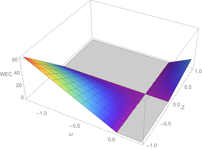
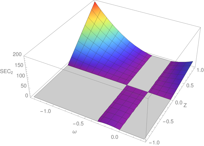
Figure 1: In this figure, we show the regions were the WEC is satisfied (left panel), and the regions were the SEC₂ is satisfied (right panel). The figures are plotted in terms of the parameters $\omega$ and $Z$, and assuming $\lambda=0.2$.

In order to study the characteristics of the matter associated with the obtained solution, it is useful to determine the conditions under which the energy density is positive, that is, the weak energy conditions (WEC). We also want to determine the requisites for the strong energy conditions (SEC) to be satisfied, i.e., for gravity to be an attractive force camenzind2007compact .

The WEC is given by

$$\rho\geq 0,$$ (19)

and, for an anisotropic fluid, the SEC is given by three inequalities, which we are going to call SEC₁, SEC₂ and SEC₃, respectively

$$\rho+p_{t}\geq 0\quad\quad\rho+p_{r}+2p_{t}\geq 0,\quad\quad\rho+p_{r}\geq 0,$$ (20)

where, the SEC₃ is trivial, since $\rho=-p_{r}$. After replacing the expressions for the energy density and the pressures in Eqs. (19) and (20), and making some simplifications, we find two inequalities that must be obeyed so that the WEC and SEC are satisfied simultaneously. These are as follows

$$Z(16\pi\omega+\lambda(1-3\omega))\geq 0$$ (21)

and

$$Z(1+3\omega)(16\pi\omega+\lambda(1-3\omega))\geq 0.$$ (22)

We can reduce Eqs. (21) and (22) to the following cases:

• If $Z=0$, the energy conditions are satisfied for:

  $$-\frac{4}{3}\leq\omega<-\frac{1}{3}.$$ (23)

• If $Z\leq 0$, the energy conditions are satisfied for:

  $$-\frac{1}{3}\leq\omega<\frac{\lambda}{3\lambda-16\pi}.$$ (24)

• If $Z\geq 0$, the energy conditions are satisfied for:

  $$\frac{\lambda}{3\lambda-16\pi}<\omega\leq\frac{1}{3}.$$ (25)

• In general, the energy conditions are also satisfied if:

  $$\omega=\frac{\lambda}{3\lambda-16\pi}.$$ (26)

In Fig. 1, the WEC (left panel) and the SEC₂ (right panel) are shown as a function of the constant of integration $Z$ and of the parameter $\omega$, for an specific choice of the coupling constant $\lambda$ of the $f(\mathbb{T},\mathcal{T})$ theory. The gray regions are the ones were the energy conditions are not satisfied, and the colorful regions are the ones were the WEC and SEC₂ are obeyed.

V Mass, horizons and temperature

We can determine the radius of the event horizon associated with the solution for the black hole by considering the region where the function $B(r)$ vanishes. Denoting $R_{h}$ as the radius of the horizon, it must satisfy the equation $B(R_{h})=0$. Thus, in terms of $R_{h}$ the black hole mass can be written as

$$M=\frac{1}{2}\left(R_{h}+ZR_{h}^{-\frac{3(16\pi\omega+\lambda(1-3\omega))}{16\pi+\lambda(1+5\omega)}}\right).$$ (27)

Equation (27) connects the mass of the black hole with the horizon. Considering Hawking radiation, a direct way to obtain the expression for this quantity is using the surface gravity of the black hole in the form

$$\kappa=\frac{1}{2}\frac{dB(r)}{dr}\Big{|}_{r=r_{h}},$$ (28)

whose result is

$$\kappa=\frac{R_{h}^{-\frac{6(8\pi+\lambda)(1+\omega)}{16\pi+\lambda(1+5\omega)}}\left((16\pi+\lambda(1+5\omega))R_{h}^{\frac{\lambda(5+\omega)+16\pi(2+3\omega)}{16\pi+\lambda(1+5\omega)}}-3Z(16\pi\omega+\lambda(1-3\omega))R_{h}\right)}{2(16\pi+\lambda(1+5\omega))}.$$ (29)

As we can see, surface gravity depends on the parameter of the equation of state $\omega$ and on the coupling constant of the $f(\mathbb{T},\mathcal{T})$ gravity, and thus, differ from the usual result in the context of GR. This implies that Hawking temperature $T=\hbar\kappa/(2\pi)$ has a similar structure and can be written in the form

$$T=\frac{\hbar}{4\pi R_{h}}-\frac{3Z\hbar(16\pi\omega+\lambda(1-3\omega))R_{h}^{-\frac{\lambda(5+\omega)+16\pi(2+3\omega)}{16\pi+\lambda(1+5\omega)}}}{4\pi(16\pi+\lambda(1+5\omega))}.$$ (30)

This temperature has correction terms due to the modified gravity as well as extra terms associated with the nature of the anisotropic fluid. In this way, it is necessary to separately analyze the influence of modified gravity and of the fluid for a given value of the horizon radius. In the next subsections we study some important values for the parameters in the expressions obtained in this section.

VI Special cases

In the next subsections, we consider some special cases for the value of the parameter $\omega$.

VI.1 Black hole surrounded by a radiation field

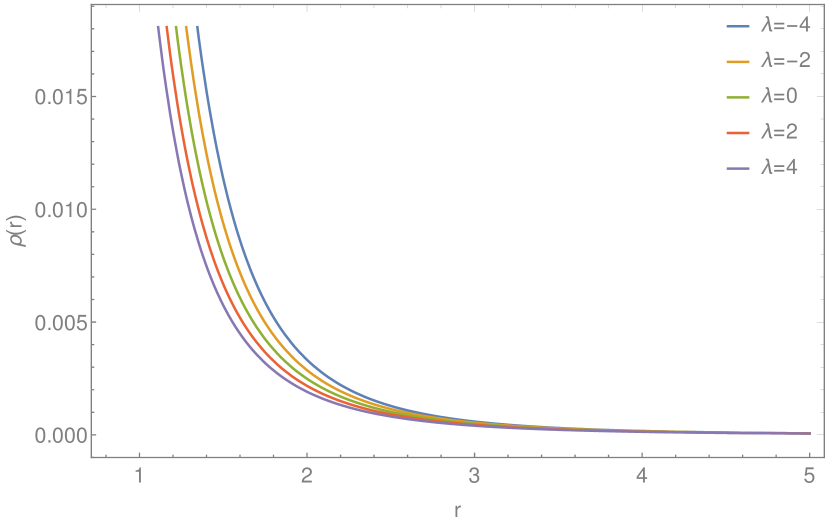
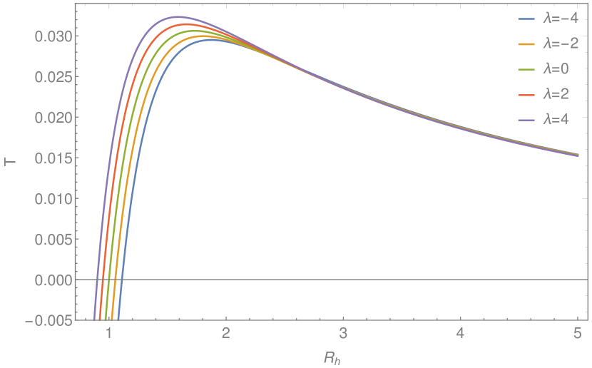
Figure 2: In this figure we show the energy density $\rho$ as a function of the radial coordinate $r$ (left panel), and the temperature $T$ as a function of the radius of the event horizon $R_{h}$ (right panel). These plots are for the case $\omega=\frac{1}{3}$ and five different values of the parameter $\lambda$, and assuming $Z=\hbar=1$.

We start considering $\omega=\frac{1}{3}$ and, in which case the metric function $B(r)$ is given by

$$B(r)=1-\frac{2M}{r}+Zr^{-\frac{12\pi+\lambda}{6\pi+\lambda}}.$$ (31)

From Eq. (31) we can observe that $B(r)$ has a dependence on the coupling constant $\lambda$, and the third term is due to the scenario in which the $f(\mathbb{T},\mathcal{T})$ is considered. The energy density in the radiation field case, is given by

$$\rho(r)=\frac{9\pi Zr^{-\frac{3(8\pi+\lambda)}{6\pi+\lambda}}}{2(6\pi+\lambda)^{2}},$$ (32)

so that, it depends on the radial coordinate and on $\lambda$. In the left panel of Fig. 2 we show $\rho(r)$ given by Eq. (32), from which conclude that the energy density diverges for $r\rightarrow 0$ and goes to zero asymptotically. The energy density decreases with the increasing of the coupling constant. As to the Hawking temperature, we find the result

$$T=\frac{\hbar}{4\pi R_{h}}-\frac{3Z\hbar R_{h}^{-\frac{2(9\pi+\lambda)}{6\pi+\lambda}}}{2(6\pi+\lambda)}.$$ (33)

From the above equation we see that $T$ changes with both $R_{h}$ and $\lambda$ and, from the right panel of Fig. 2 we can conclude that the temperature diverges when $R_{h}\rightarrow 0$, then it increases with the increasing of $R_{h}$ until it reaches a maximum and then starts to decrease again. For a fixed radius of the event horizon, the temperature increases with the increasing of $\lambda$.

VI.2 Black hole surrounded by a dust field

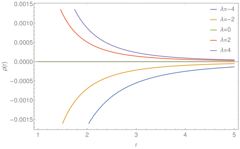
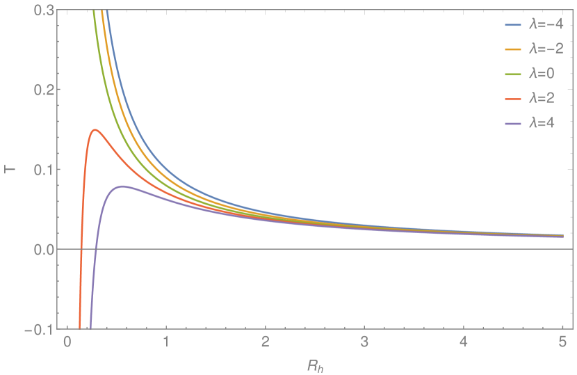
Figure 3: In this figure we show the energy density $\rho$ as a function of the radial coordinate $r$ (left panel), and the temperature $T$ as a function of the radius of the event horizon $R_{h}$ (right panel). These plots are for the case $\omega=0$ and five different values of the parameter $\lambda$, and assuming $Z=\hbar=1$.

Here we analyze the case $\omega=0$ and, obtain the following solution for $B(r)$

$$B(r)=1-\frac{2M}{r}+Zr^{-\frac{4(4\pi+\lambda)}{16\pi+\lambda}}.$$ (34)

From the above equation we see that the metric function $B(r)$ codifies the influence of the context we are considering, namely, the $f\left(\mathbb{T},\mathcal{T}\right)$ gravity. As expected, the energy density is also modified by the theory, and it is given by

$$\rho(r)=\frac{6\lambda Zr^{-\frac{6(8\pi+\lambda)}{16\pi+\lambda}}}{(16\pi+\lambda)^{2}}.$$ (35)

The left panel of Fig. 3 shows how the energy density behaves with $r$ and $\lambda$ for the $\omega=0$ case. For the GR case $(\lambda=0)$ there is no field surrounding the black hole since we have $\rho(r)=0$. For positive values of $\lambda$ the energy density diverges for $r\rightarrow 0$ and tends to zero from above for increasing values of the radial coordinate. When we consider negative values of $\lambda$, we obtain $\rho\rightarrow-\infty$ when $r$ goes to zero, and $\rho$ tends to zero from below when $r$ increases. For a fixed value of $r$, $\rho$ increases with the increasing of $\lambda$. The temperature in the present case is as follows

$$T=\frac{\hbar}{4\pi R_{h}}-\frac{3\lambda Z\hbar R_{h}^{-\frac{32\pi+5\lambda}{16\pi+\lambda}}}{4\pi(16\pi+\lambda)}.$$ (36)

From the right panel of Fig. 3 we can observe that when $R_{h}$ goes to zero, the temperature diverges to $-\infty$ for positive values of $\lambda$, and to $+\infty$ for negative values of $\lambda$ and for $\lambda=0$. As $R_{h}$ increases, $T$ assumes positive values for all the choices of the coupling constant, and goes to zero as the horizon radius increases. In general, $T$ increases with the decreasing of $\lambda$.

VI.3 Black hole surrounded by a cosmological constant field

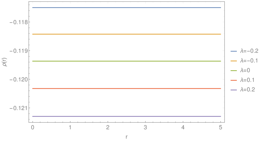
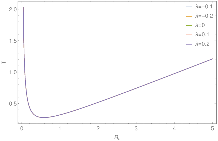
Figure 4: In this figure we show the energy density $\rho$ as a function of the radial coordinate $r$ (left panel), and the temperature $T$ as a function of the radius of the event horizon $R_{h}$ (right panel). These plots are for the case $\omega=-1$ and five different values of the parameter $\lambda$, and assuming $Z=\hbar=1$.

Here we analyze the special case $\omega=-1$. For this choice of $\omega$, $B(r)$ is given by

$$B(r)=1-\frac{2M}{r}+Zr^{2}.$$ (37)

In Eq. (37) we can observe that in this case the solution for the metric is the same as the one obtained by Kiselev in GR kiselev . In this case, the result obtained in the framework of the $f\left(\mathbb{T},\mathcal{T}\right)$ gravity is analogous to the one obtained by Kiselev kiselev . This behavior was also observed in Rastall gravity heydarzade2017black and in $f(R,T)$ santos2023kiselev . Despite having the same metric solution as in GR, the energy density is modified according to

$$\rho(r)=-\frac{3Z}{8\pi-2\lambda}.$$ (38)

We can conclude from the above equation that the energy density is inversely proportional to the $f\left(\mathbb{T},\mathcal{T}\right)$ coupling constant $\lambda$, but it does not depend on the radial coordinate, as can be seem on the left panel of Fig. 4. The Hawking temperature for this case is as follows

$$T=\frac{\hbar}{4\pi R_{h}}+\frac{3Z\hbar R_{h}}{4\pi}.$$ (39)

It is interesting to notice that $T$ also does not depend on the modified theory of gravity taken into account, in which case the Hawking temperature only varies with $R_{h}$. As shown in the right panel of Fig. 4, $T$ will diverge for $R_{h}\rightarrow 0$, then for increasing values of $R_{h}$ the temperature decreases until it reaches a minimum, and then it starts to increase again with the increasing of the radius of the event horizon.

VI.4 Black hole surrounded by a quintessence field

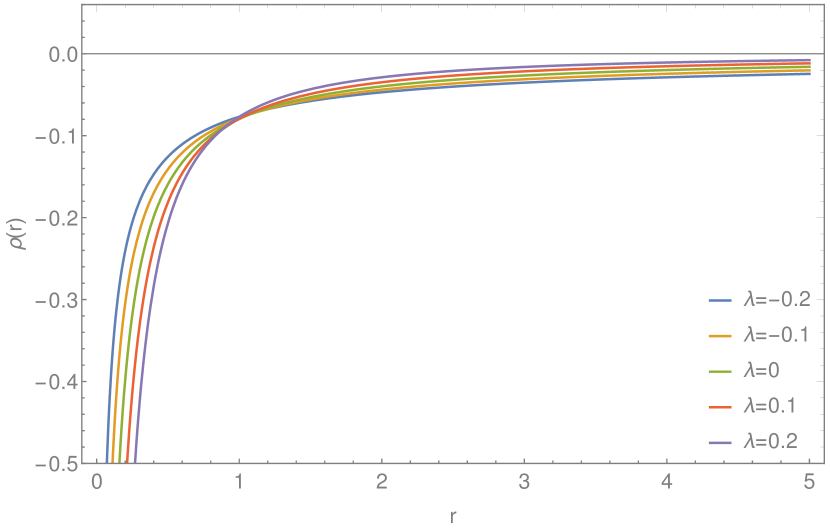
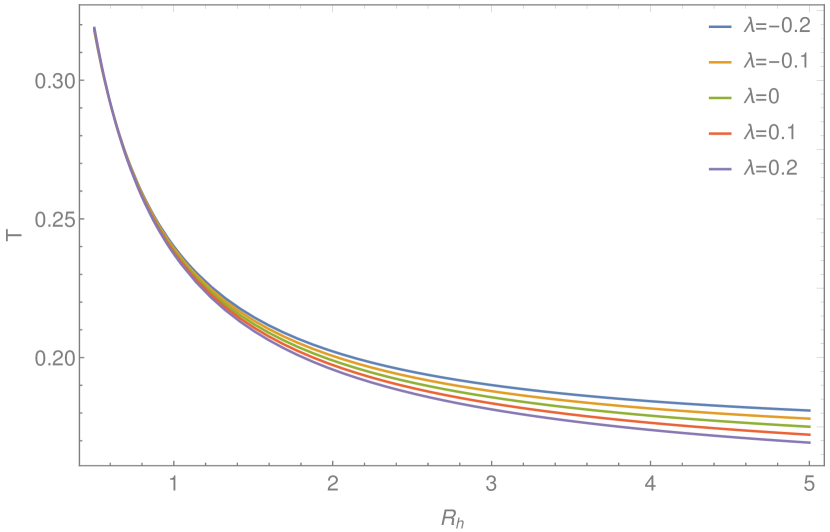
Figure 5: In this figure we show the energy density $\rho$ as a function of the radial coordinate $r$ (left panel), and the temperature $T$ as a function of the radius of the event horizon $R_{h}$ (right panel). These plots are for the case $\omega=\frac{2}{3}$ and five different values of the parameter $\lambda$, and assuming $Z=\hbar=1$.

Let us now consider the special case $\omega=-2/3$, for this choice of value for the parameter $\omega$, the metric function $B(r)$ is

$$B(r)=1-\frac{2M}{r}+Zr^{-\frac{48\pi-20\lambda}{48\pi-7\lambda}}.$$ (40)

We can conclude from the above equation that in this case too the spacetime metric codifies the role played by the modified theory of gravity. The energy density for this case is as follows

$$\rho(r)=-\frac{18(32\pi-9\lambda)Zr^{-\frac{6(8\pi+\lambda)}{48\pi-7\lambda}}}{(48\pi-7\lambda)^{2}}.$$ (41)

In the left panel of Fig. 5 we show the plots of the energy density as a function of the radial coordinate. We can observe that the energy density does not satisfy the energy conditions for none of the values of $\lambda$ analyzed, which is in accordance with the analysis made in Section IV. As for the Hawking temperature, it is given by

$$T=\frac{\hbar}{4\pi R_{h}}+\frac{3(32\pi-9\lambda)Z\hbar R_{h}^{-\frac{13\lambda}{48\pi-7\lambda}}}{4\pi(48\pi-7\lambda)}.$$ (42)

We can observe in the right panel of Fig. 5 that for all values of the parameter $\lambda$, $T$ diverges when $R_{h}\rightarrow 0$, and then decreases with the increasing of $R_{h}$. Also, for this case, the temperature decreases with the increasing of the parameter of the modified teleparallel gravity.

VI.5 Black hole surrounded by a phantom field

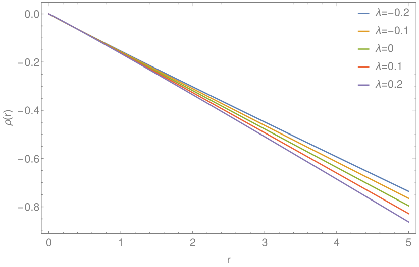
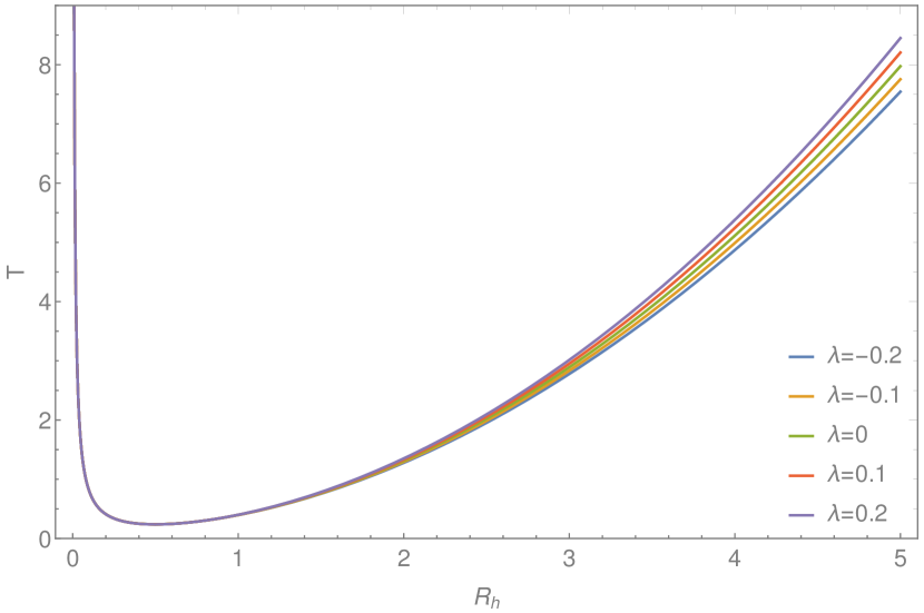
Figure 6: In this figure we show the energy density $\rho$ as a function of the radial coordinate $r$ (left panel), and the temperature $T$ as a function of the radius of the event horizon $R_{h}$ (right panel). These plots are for the case $\omega=\frac{4}{3}$ and five different values of the parameter $\lambda$, and assuming $Z=\hbar=1$.

Lastly, we study the case $\omega=-\frac{4}{3}$, for this choice of $\omega$ the metric function $B(r)$ is given by the following expression

$$B(r)=1-\frac{2M}{r}+Zr^{\frac{4(36\pi-7\lambda)}{48\pi-17\lambda}}.$$ (43)

From the above equation, we conclude that for $\omega=-4/3$, the metric is also affected the fact that we are in the framework of a the modified theory. As for the energy density, it is given by

$$\rho(r)=-\frac{18(64\pi-15\lambda)Zr^{\frac{6(8\pi+\lambda)}{48\pi-17\lambda}}}{(48\pi-17\lambda)^{2}}.$$ (44)

As in the previous subsection, in this case, we also can observe from the left panel of Fig. 6 that in any of the cases analyzed $\rho(r)$ satisfies the energy conditions. This was also expected from the analysis made in Section IV. The temperature for this choice of value for $\omega$ is

$$T=\frac{\hbar}{4\pi R_{h}}+\frac{3(64\pi-15\lambda)Z\hbar R_{h}^{\frac{96\pi-11\lambda}{48\pi-17\lambda}}}{4\pi(48\pi-17\lambda)}.$$ (45)

In the right panel of Fig. 6, we can see that $T$ diverges when $R_{h}$ goes to zero, then as the event horizon radius increases the temperature decreases until it reaches a minimum, and then it stars the increase again. For this case, we conclude that the temperature increases with the increasing of the parameter $\lambda$.

VII Final Remarks

In this work we obtained the solution in gravity $f(\mathbb{T},\mathcal{T})$ that corresponds to an extension of the Kiselev black hole to the framework of the $f(\mathbb{T},\mathcal{T})$ gravity. Our strategy consists in identifying the fluid under consideration as an anisotropic fluid and mapping the components of the Kiselev energy–momentum tensor into the corresponding energy–momentum tensor of the anisotropic fluid. This approach allows us to identify the Lagrangian associated with the fluid and consequently write the field equations for this physical system. We have assume that the function $f(\mathbb{T},\mathcal{T})=\lambda\mathbb{T}\mathcal{T}$, where $\lambda$ is a coupling constant of geometry with matter fields. This particular form of $f(\mathbb{T},\mathcal{T})$ allows us to obtain an exact solution for the field equation on this theory. The general solution obtained represented by Eq. (17) carries dependence on the coupling constant and on the parameter of the equation of state. Thus, the presence of modified gravity adds additional terms to the line element that represents the geometry of spacetime associated to an extension of the Kiselev black hole, in the framework of $f(\mathbb{T},\mathcal{T})$ gravity.

For this class of solution of the modified field equation, it is possible to explicitly determine the form of the energy density and consequently the radial and tangential pressures by using the equation of state. As we can see in Eq. (18), the energy density has a general expression in which its behavior can vary greatly, depending on the choice of constituent parameters. In this way, we separately analyze certain values for the parameter of the equation of state. In the same way, we study the general form for the Hawking temperature and analyze some particular values for the parameter of the equation of state. In general, for all special cases analyzed the Hawking temperature goes in the opposite direction than the energy density in relation to the $f(\mathbb{T},\mathcal{T})$ parameter. That is, when $\rho$ increases with $\lambda$, $T$ decreases, and vice-versa, except for the case $\omega=-1$, where the temperature does not varies with $\lambda$. We also concluded that the energy conditions were only satisfied for the cases $\omega=1/3$ and $\omega=0$. As also observed in other modified theories heydarzade2017black ; santos2023kiselev , in the case $\omega=-1$ the spacetime metric is not changed by the modified theory of gravity.

The solution obtained in the present work can be used in future works to study other physical quantities such as geodesics associated with light path and massive bodies in addition to the thermodynamics of this black hole considering criticality and efficiency. The rotating black hole solution surrounded by a Kiselev fluid in $f(\mathbb{T},\mathcal{T})$ gravity is another example of future work based on our results.

References

- (1) K. Akiyama, A. Alberdi, W. Alef, J. C. Algaba, R. Anantua, K. Asada, R. Azulay, U. Bach, A.-K. Baczko, D. Ball, et al., “First Sagittarius A* Event Horizon Telescope results. I. The shadow of the supermassive black hole in the center of the Milky Way,” The Astrophysical Journal Letters, vol. 930, no. 2, p. L12, 2022.
- (2) G. A. González and P. S. Letelier, “Rotating relativistic thin disks,” Physical Review D, vol. 62, no. 6, p. 064025, 2000.
- (3) J. P. S. Lemos and P. S. Letelier, “Exact general relativistic thin disks around black holes,” Physical Review D, vol. 49, no. 10, p. 5135, 1994.
- (4) O. Semerák and P. Suková, “Free motion around black holes with discs or rings: between integrability and chaos–I,” Monthly Notices of the Royal Astronomical Society, vol. 404, no. 2, pp. 545–574, 2010.
- (5) M. E. Rodrigues, M. V. S. Silva, and H. A. Vieira, “Bardeen-Kiselev black hole with a cosmological constant,” Physical Review D, vol. 105, no. 8, p. 084043, 2022.
- (6) A. Younas, M. Jamil, S. Bahamonde, and S. Hussain, “Strong gravitational lensing by Kiselev black hole,” Physical Review D, vol. 92, no. 8, p. 084042, 2015.
- (7) V. B. Bezerra, L. C. N. Santos, F. M. da Silva, and H. Moradpour, “On black holes surrounded by a fluid of strings in Rastall gravity,” General Relativity and Gravitation, vol. 54, no. 9, p. 109, 2022.
- (8) J. P. M. Graça, E. F. Capossoli, H. Boschi-Filho, and I. P. Lobo, “Joule-Thomson expansion for quantum corrected AdS-Reissner-Nördstrom black holes in a Kiselev spacetime,” Physical Review D, vol. 107, no. 2, p. 024045, 2023.
- (9) A. De Felice and S. Tsujikawa, “f(R) theories,” Living Reviews in Relativity, vol. 13, no. 1, pp. 1–161, 2010.
- (10) T. Harko, F. S. N. Lobo, S. Nojiri, and S. D. Odintsov, “ gravity,” Physical Review D, vol. 84, no. 2, p. 024020, 2011.
- (11) P. Rastall, “Generalization of the Einstein theory,” Physical Review D, vol. 6, no. 12, p. 3357, 1972.
- (12) C. E. Mota, L. C. N. Santos, F. M. da Silva, G. Grams, I. P. Lobo, and D. P. Menezes, “Generalized Rastall’s gravity and its effects on compact objects,” International Journal of Modern Physics D, vol. 31, no. 04, p. 2250023, 2022.
- (13) F. M. da Silva, L. C. N. Santos, C. E. Mota, T. O. F. da Costa, and J. C. Fabris, “Rapidly rotating neutron stars in f(R,T)=R+2T gravity,” The European Physical Journal C, vol. 83, no. 4, p. 295, 2023.
- (14) L. C. N. Santos and V. B. Bezerra, “Electrostatic self-interaction of a charged particle in the space-time of a cosmic string in the context of gravity’s rainbow,” General Relativity and Gravitation, vol. 51, pp. 1–8, 2019.
- (15) K. Hayashi and T. Shirafuji, “New general relativity,” Physical Review D, vol. 19, no. 12, p. 3524, 1979.
- (16) R. Aldrovandi and J. G. Pereira, Teleparallel gravity: an introduction, vol. 173. Springer Science & Business Media, 2012.
- (17) J. W. Maluf, “The teleparallel equivalent of general relativity,” Annalen der Physik, vol. 525, no. 5, pp. 339–357, 2013.
- (18) T. Harko, F. S. N. Lobo, G. Otalora, and E. N. Saridakis, “ gravity and cosmology,” Journal of Cosmology and Astroparticle Physics, vol. 2014, no. 12, p. 021, 2014.
- (19) S. Bahamonde, C. G. Böhmer, and M. Krššák, “New classes of modified teleparallel gravity models,” Physics Letters B, vol. 775, pp. 37–43, 2017.
- (20) S. G. Vilhena, S. B. Duarte, M. Dutra, and P. J. Pompeia, “Neutron stars in modified teleparallel gravity,” Journal of Cosmology and Astroparticle Physics, vol. 2023, no. 04, p. 044, 2023.
- (21) V. V. Kiselev, “Quintessence and black holes,” Classical and Quantum Gravity, vol. 20, p. 1187, mar 2003.
- (22) R. A. Konoplya, “Shadow of a black hole surrounded by dark matter,” Physics Letters B, vol. 795, pp. 1–6, 2019.
- (23) X.-X. Zeng and H.-Q. Zhang, “Influence of quintessence dark energy on the shadow of black hole,” The European Physical Journal C, vol. 80, no. 11, pp. 1–14, 2020.
- (24) A. Abdujabbarov, B. Toshmatov, Z. Stuchlík, and B. Ahmedov, “Shadow of the rotating black hole with quintessential energy in the presence of plasma,” International Journal of Modern Physics D, vol. 26, no. 06, p. 1750051, 2017.
- (25) A. He, J. Tao, Y. Xue, and L. Zhang, “Shadow and photon sphere of black hole in clouds of strings and quintessence,” Chinese Physics C, 2022.
- (26) B. B. Thomas, M. Saleh, and T. C. Kofane, “Thermodynamics and phase transition of the Reissner–Nordström black hole surrounded by quintessence,” General Relativity and Gravitation, vol. 44, no. 9, pp. 2181–2189, 2012.
- (27) K. Ghaderi and B. Malakolkalami, “Thermodynamics of the Schwarzschild and the Reissner–Nordström black holes with quintessence,” Nuclear Physics B, vol. 903, pp. 10–18, 2016.
- (28) M. Saleh, B. B. Thomas, and T. C. Kofane, “Thermodynamics and phase transition from regular Bardeen black hole surrounded by quintessence,” International Journal of Theoretical Physics, vol. 57, no. 9, pp. 2640–2647, 2018.
- (29) J. M. Toledo and V. B. Bezerra, “Some remarks on the thermodynamics of charged AdS black holes with cloud of strings and quintessence,” The European Physical Journal C, vol. 79, no. 2, pp. 1–11, 2019.
- (30) H. Chen, B. C. Lütfüoğlu, H. Hassanabadi, and Z.-W. Long, “Thermodynamics of the Reissner-Nordström black hole with quintessence matter on the EGUP framework,” Physics Letters B, vol. 827, p. 136994, 2022.
- (31) R. Tharanath and V. C. Kuriakose, “Thermodynamics and spectroscopy of Schwarzschild black hole surrounded by quintessence,” Modern Physics Letters A, vol. 28, no. 04, p. 1350003, 2013.
- (32) M.-S. Ma, R. Zhao, and Y.-Q. Ma, “Thermodynamic stability of black holes surrounded by quintessence,” General Relativity and Gravitation, vol. 49, no. 6, pp. 1–20, 2017.
- (33) Z. Xu, Y. Liao, and J. Wang, “Thermodynamics and phase transition in rotational Kiselev black hole,” International Journal of Modern Physics A, vol. 34, no. 30, p. 1950185, 2019.
- (34) S. Chen and J. Jing, “Quasinormal modes of a black hole surrounded by quintessence,” Classical and Quantum Gravity, vol. 22, no. 21, p. 4651, 2005.
- (35) Y. Zhang and Y.-X. Gui, “Quasinormal modes of gravitational perturbation around a Schwarzschild black hole surrounded by quintessence,” Classical and Quantum Gravity, vol. 23, no. 22, p. 6141, 2006.
- (36) N. Varghese and V. C. Kuriakose, “Quasinormal modes of Reissner–Nördstrom black hole surrounded by quintessence,” General Relativity and Gravitation, vol. 41, no. 6, pp. 1249–1257, 2009.
- (37) Y. Zhang, Y. Gui, F. Yu, and F. Li, “Quasinormal modes of a Schwarzschild black hole surrounded by free static spherically symmetric quintessence: electromagnetic perturbations,” General Relativity and Gravitation, vol. 39, no. 7, pp. 1003–1010, 2007.
- (38) J. Rayimbaev, B. Majeed, M. Jamil, K. Jusufi, and A. Wang, “Quasiperiodic oscillations, quasinormal modes and shadows of Bardeen–Kiselev Black Holes,” Physics of the Dark Universe, vol. 35, p. 100930, 2022.
- (39) J. M. Toledo and V. B. Bezerra, “The Reissner–Nordström black hole surrounded by quintessence and a cloud of strings: thermodynamics and quasinormal modes,” International Journal of Modern Physics D, vol. 28, no. 01, p. 1950023, 2019.
- (40) M. Saleh, B. T. Bouetou, and T. C. Kofane, “Quasinormal modes and Hawking radiation of a Reissner-Nordström black hole surrounded by quintessence,” Astrophysics and Space Science, vol. 333, no. 2, pp. 449–455, 2011.
- (41) R. Tharanath, N. Varghese, and V. C. Kuriakose, “Phase transition, quasinormal modes and Hawking radiation of Schwarzschild black hole in quintessence field,” Modern Physics Letters A, vol. 29, no. 11, p. 1450057, 2014.
- (42) M. Saleh, B. B. Thomas, and T. C. Kofane, “Quasinormal modes of gravitational perturbation around regular Bardeen black hole surrounded by quintessence,” The European Physical Journal C, vol. 78, no. 4, pp. 1–7, 2018.
- (43) D. Deb, S. V. Ketov, S. K. Maurya, M. Khlopov, P. H. R. S. Moraes, and S. Ray, “Exploring physical features of anisotropic strange stars beyond standard maximum mass limit in gravity,” Monthly Notices of the Royal Astronomical Society, vol. 485, no. 4, pp. 5652–5665, 2019.
- (44) I. G. Salako, M. Khlopov, S. Ray, M. Arouko, P. Saha, and U. Debnath, “Study on anisotropic strange stars in gravity,” Universe, vol. 6, no. 10, p. 167, 2020.
- (45) C. E. Mota, L. C. N. Santos, F. M. da Silva, C. V. Flores, T. J. N. da Silva, and D. P. Menezes, “Anisotropic compact stars in Rastall–Rainbow gravity,” Class. Quant. Grav., vol. 39, no. 8, p. 085008, 2022.
- (46) M. Camenzind, Compact objects in astrophysics. Springer, 2007.
- (47) Y. Heydarzade and F. Darabi, “Black hole solutions surrounded by perfect fluid in Rastall theory,” Physics Letters B, vol. 771, pp. 365–373, 2017.
- (48) L. C. N. Santos, F. M. da Silva, C. E. Mota, I. P. Lobo, and V. B. Bezerra, “Kiselev black holes in f(R,T) gravity,” General Relativity and Gravitation, vol. 55, no. 8, p. 94, 2023.