Two-dimensional solitons in second-harmonic-generating media with fractional diffraction

Abstract

We introduce a system of propagation equations for the fundamental-frequency (FF) and  second-harmonic (SH) waves in the bulk waveguide with the effective fractional diffraction and quadratic ($\chi^{(2)}$) nonlinearity. The numerical solution produces families of ground-state (zero-vorticity) two-dimensional solitons in the free space, which are stable in exact agreement with the Vakhitov-Kolokolov criterion, while vortex solitons are completely unstable in that case. Mobility of the stable solitons and inelastic collisions between them are briefly considered too. In the presence of a harmonic-oscillator (HO) trapping potential, families of partially stable single- and two-color solitons (SH-only or FF-SH ones, respectively) are obtained, with zero and nonzero vorticities. The single- and two-color solitons are linked by a bifurcation which takes place with the increase of the soliton’s power.

I Introduction

Fractional derivatives have been known since long ago as a formal extension of the classical calculus. A broadly accepted definition is one of the Caputo derivative of non-integer order $\alpha$ [2, 1],

$$D_{x}^{\alpha}\psi(x)=\frac{1}{\Gamma\left(1-\{\alpha\}\right)}\int_{0}^{x}\frac{f^{\left(n\right)}(\xi)dx}{\left(x-\xi\right)^{\left\{\alpha\right\}}},$$ (1)

where $n\equiv[\alpha]+1$, $[\alpha]$ and $\{\alpha\}$ being the integer and fractional parts of $\alpha$, $\Gamma$ is the Gamma-function, and $f^{(n)}$ is the usual derivative. Note that this definition represents the fractional derivative as the integral (nonlocal) operator, rather than as a differential one. In physics, fractional differential operators were introduced as the basis of the Laskin’s fractional quantum mechanics for particles whose classical motion is performed by Lévy flights [3, 4, 5]. While experimental realization of this theory has not been reported yet, it was proposed by Longhi to emulate the fractional Schrödinger equation in optics, making use of the well-known similarity of the quantum-mechanical Schrödinger equation and the equation for the paraxial propagation of light. Thus, the action of the fractional kinetic-energy operator in the quantum theory can be emulated by means of the effective fractional diffraction in optics [6]. The proposal was based on using an optical cavity, decomposing the light beam into transverse Fourier components and passing them through an appropriate phase shifter, which imposes phase changes corresponding to the expected effect of the fractional diffraction. Eventually, the Fourier components are recombined back into a single optical beam. While the action of this setup is discrete, circulation of the beam in the cavity is approximated by the continuous fractional Schrödinger equation.

The experimental implementation of the emulated fractional diffraction in optics has not yet been reported either. However, a similar effect, in the form of effective fractional group-velocity dispersion (GVD) in a fiber cavity, has been reported in Ref. [7]. It used the decomposition of the optical pulse in the temporal domain into its spectral components, which were given phase shifts, emulating the fractional GVD, by passing them through an appropriate phase plate (hologram).

The realization of the fractional diffraction or dispersion in optical systems suggests to take into regard intrinsic nonlinearity of the material, thus introducing various forms of the fractional nonlinear Schrödinger (FNLS) equation. These models give rise to diverse species of fractional solitons and related phenomena, that include accessible [8], gap [9, 10, 11], and lattice [15, 12, 13] solitons, breathers [18], vortices [15, 16], wave collapse [17], spontaneous symmetry breaking [18, 19], nonlinear couplers [20, 21, 22], spin-orbit-coupled systems [23, 24], etc. In addition to these models formulated in the 1D and 2D spatial domains, fractional spatiotemporal models with the nonlocal nonlinearity of the “accessible” type and various potentials were introduced in terms of spherical coordinates [25, 26, 27]. These theoretical results were reviewed in Refs. [28], [29], and [30]. Very recently, the first experimental realization of nonlinear effects in a fiber cavity with fractional GVD was reported, in the form of bifurcations of spectral peaks [31].

The above-mentioned works considered the interplay of the fractional diffraction/dispersion with the ubiquitous cubic ($\chi^{(3)}$) term in the framework of the FNLS equation. Another generic species of the optical nonlinearity, of the $\chi^{(2)}$ type, represents the second-harmonic (SH) generation by quadratic terms, in the framework of coupled equations for the fundamental-frequency (FF) and SH waves [32, 33, 34, 35]. The system of the one-dimensional (1D) FF-SH equations, coupled by $\chi^{(2)}$ terms, with the fractional diffraction acting on both the FF and SH components, was recently introduced in Ref. [36], where existence and stability conditions for fundamental solitons generated by this system were identified by means of numerical calculations.

In this connection, it is relevant to mention that a model based on the single one-dimensional FNLS equation, combining the cubic self-repulsive and quadratic attractive terms, was investigated in another recent work [37]. This combined nonlinearity appears in the effective 1D Gross-Pitaevskii (GP) equation for identical wave functions of two components of the binary Bose-Einstein condensate (BEC), which takes into regard the effective repulsive mean-field interaction and the correction produced by effects of quantum fluctuations [38]. The quadratic-cubic fractional GP equation introduced in Ref. [37] is, presumably, a relevant model for the quasi-1D BEC of particles which move by Lévy flights, obeying the above-mentioned fractional Schrödinger equation in the single-particle limit. Soliton families, produced by this fractional GP equation, and their stability were studied in Ref. [37], including bound states of fundamental solitons supported by the lattice modulation of the quadratic term.

The objective of the present work is to introduce a two-dimensional (2D) system of equations for the FF and SH waves with the optical $\chi^{\left(2\right)}$ nonlinearity and fractional diffraction acting in both equations. The consideration of this system  is definitely relevant – in particular, because stable spatial optical solitons supported by the $\chi^{(2)}$ nonlinearity (in the case of the normal non-fractional diffraction) were first created in the (2+1)D form [32]. We consider the system in the free space, and separately in the presence of a 2D harmonic-oscillator (HO) trapping potential. Using numerical methods, we construct families of 2D ground-state (GS, alias zero-vorticity) and vortex solitons and identify their stability. In the free space, the stability of the GS solitons exactly obeys the celebrated Vakhitov-Kolokolov (VK ) criterion [39, 40] (its precise form is defined below), while the vortex solitons are unstable, as may be expected from the comparison with known results for vortex solitons in the case of the non-fractional diffraction [41, 42]. The HO potential may provide stabilization for various modes – in particular, for the “single-color” bound states which contain solely the SH component, while the FF one is zero, as well as for the “two-color” modes including both components. In spite of the apparent simplicity of the former states, their stability is not obvious, as it is affected by the $\chi^{(2)}$ coupling of small perturbations in the FF component to the underlying SH field, which may give rise to the parametric instability [43]. Furthermore, we demonstrate that the trapping potential provides partial stabilization for vortex states as well, of both the single- and two-color types.

The paper is organized as follows. The model is introduced in Section II, which is followed in Section III by systematic presentation of results for soliton families and their stability in the free space (as mentioned above, the stability of the GS solitons fully agrees with the Vakhitov-Kolokolov criterion). Section III also briefly examines mobility of stable fundamental solitons and collisions between them. The results for single- and two-color fundamental and vortex solitons supported by the HO potential are reported in Section IV. The paper is concluded by Section V.

II The model

The system of coupled 2D equations for the spatial-domain evolution of amplitudes $U\left(x,y,z\right)$ and $W\left(x,y,z\right)$ of the FF and SH waves in the bulk optical waveguide with fractional diffraction is

$$i\frac{\partial U}{\partial z} = \frac{1}{2}\left(-\frac{\partial^{2}}{\partial x^{2}}-\frac{\partial^{2}}{\partial y^{2}}\right)^{\alpha/2}U-WU^{\ast},$$ (2)

$$2i\frac{\partial W}{\partial z} = \frac{1}{2}\left(-\frac{\partial^{2}}{\partial x^{2}}-\frac{\partial^{2}}{\partial y^{2}}\right)^{\alpha/2}W+QW-\frac{1}{2}U^{2}.$$ (3)

Here $\left(x,y\right)$ are the transverse coordinates, $z$ is the propagation distance, real $Q$ is the mismatch parameter, which can be reduced, by rescaling, to one of three values,

$$Q=\pm 1\text{ {or~{}}}Q=0,$$ (4)

and $\ast$ stands for the complex conjugate.

The present system is introduced as a natural 2D extension of the 1D fractional $\chi^{(2)}$ system that was elaborated in Ref. [36]. According to the above-mentioned derivation [6], the fractional-diffraction operator is represented by the 2D version of the Riesz derivative [44, 45] with Lévy index (LI) $\alpha$, viz.,

$$\left(-\frac{\partial^{2}}{\partial x^{2}}-\frac{\partial^{2}}{\partial y^{2}}\right)^{\alpha/2}U(x)=\frac{1}{\left(2\pi\right)^{2}}\int_{-\infty}^{+\infty}dp\int_{-\infty}^{+\infty}dq\left(p^{2}+q^{2}\right)^{\alpha/2}\int_{-\infty}^{+\infty}d\xi\int_{-\infty}^{+\infty}d\eta e^{ip(x-\xi)+iq(y-\eta)}U(\xi,\eta).$$ (5)

The usual and fractional diffraction corresponds, respectively, to $\alpha=2$ and $\alpha<2$. A straightforward estimate demonstrates that the $\chi^{(2)}$ system of 2D equations (2) and (3) gives rise to the collapse (catastrophic self-compression leading to appearance of singularities [40]) at $\alpha\leq 1$, hence the system may give rise to stable solitons in the interval of

$$1<\alpha\leq 2$$ (6)

(the 1D version of the fractional $\chi^{(2)}$ system supports stable soliton in the interval of $1/2<\alpha\leq 2$). On the other hand, the 2D FNLS equation with the cubic self-focusing term gives rise to the collapse at all values of $\alpha\leq 2$, hence it cannot support stable solitons in any case [17, 28]).

It is relevant to stress that the conclusion of the collapse avoidance in interval (6) is valid for the free space. If a trapping potential is added to Eqs. (2) and (3). stability of the localized modes may be extended to the region of $\alpha\leq 1$, as demonstrated below.

Stationary solutions to Eqs. (2) and (3) with FF and SH propagation constants $k>0$ and $2k$ are looked for as

$$U\left(x,y,z\right)=e^{ikz}u(x,y),W\left(x,y,z\right)=e^{2ikz}w(x,y),$$ (7)

where functions $u$ and $w$ satisfy the following system of stationary equations:

$$-ku = \frac{1}{2}\left(-\frac{\partial^{2}}{\partial x^{2}}-\frac{\partial^{2}}{\partial y^{2}}\right)^{\alpha/2}u-wu^{\ast},$$ (8)

$$-4kw = \frac{1}{2}\left(-\frac{\partial^{2}}{\partial x^{2}}-\frac{\partial^{2}}{\partial y^{2}}\right)^{\alpha/2}w+Qw-\frac{1}{2}u^{2}.$$ (9)

Stationary localized solutions are naturally characterized by the total power, which is a dynamical invariant of Eqs. (2) and (3):

$$P=\int_{-\infty}^{+\infty}dx\int_{-\infty}^{+\infty}dy(|u|^{2}+4|w|^{2}).$$ (10)

Axisymmetric stationary solutions of Eqs. (8) and (9) are sought for, in terms of polar coordinates $\left(r,\theta\right)$, as

$$u\left(r,\theta\right)=u_{m}(r)e^{im\theta},~{}w\left(r,\theta\right)=w_{m}(r)e^{2im\theta},$$ (11)

where $u_{m}(r)$ and $w_{m}(r)$ are real radial functions, and integer $m=0,\pm 1,\pm 2\,...$ is the vorticity (alias the winding number) of the FF component. Then, the SH winding number is $2m$, as determined by Eq. (9). In addition to the power (10), the stationary states are characterized by the angular momentum,

$$M=2\pi m^{2}\int_{0}^{\infty}rdr\left[u_{m}^{2}(r)+8w_{m}^{2}(r)\right],$$ (12)

which also represents a dynamical invariant of the underlying system.

Lastly, the system’s Hamiltonian, which is conserved too, is written in terms of stationary fields $u$ and $w$ as

$$H=\frac{1}{\left(2\pi\right)^{2}}\int_{0}^{+\infty}dp\int_{0}^{+\infty}dq\left(p^{2}+q^{2}\right)^{\alpha/2}\int_{-\infty}^{+\infty}dx\int_{-\infty}^{+\infty}dy\int_{-\infty}^{+\infty}d\xi\int_{-\infty}^{+\infty}d\eta$$

$$\times\cos\left[p\left(x-\xi\right)\right]\cos\left[q\left(y-\eta\right)\right]\left[u^{\ast}\left(x,y\right)u\left(\xi,\eta\right)+w^{\ast}\left(x,y\right)w\left(\xi,\eta\right)\right]$$

$$+\int_{-\infty}^{+\infty}dx\int_{-\infty}^{+\infty}dy\left\{\left[\frac{Q}{2}\left|w\right|^{2}\right]-\frac{1}{4}\left[w\left(u^{\ast}\right)^{2}+w^{\ast}u^{2}\right]\right\},$$ (13)

where the complex structure of the fractional-diffraction terms corresponds to the definition (5). Note that this structure secures that $H$ is always real.

In the case of zero mismatch, $Q=0$ (see Eq. (4)), it follows from Eqs. (8) and (9) that amplitudes $U_{0}=u_{0}(r=0)$ and $W_{0}=w_{0}(r=0)$ of real solutions for GS axisymmetric solitons (11) with $m=0$, their characteristic radial size $R$, and the corresponding power (10) satisfy exact scaling relations for the variation of $k$:

$$U_{0}(Q=0),W_{0}\left(Q=0\right)\sim k,~{}R\left(Q=0\right)\sim k^{-1/\alpha},~{}P(Q=0)\sim k^{2(1-1/\alpha)}.$$ (14)

In the presence of the mismatch, i.e., with $Q=\pm 1$ in Eq. (4), the scaling relations (14) are asymptotically valid for $k\gg 1$, i.e., for narrow solitons with $R\ll 1$, as confirmed below by Fig. 2(b).

In the interval of LI values (6), relation $P\left(k\right)$, as given by Eq. (14), satisfies the above-mentioned VK criterion, which takes the form of $dP/dk>0$. It is the universal necessary stability condition for localized modes maintained by any self-attractive nonlinearity. The fact that the $\chi^{(2)}$ nonlinearity may be considered as the attractive self-interaction follows from the fact that, in the GS states produced by Eqs. (2) and (3), the real $w$ component is positive (see Fig. 1(a) below), hence the $\chi^{(2)}$ term in Hamiltonian (13) is negative, which indeed implies the self-attraction.

Precisely at $\alpha=1$, Eq. (14) yields $dP/dk=0$, implying the occurrence of the critical collapse, which takes place in the framework of the system of equations (2) and (3) if the power of the initial condition exceeds a certain critical value [40]. At $\alpha<1$, Eq. (14) yields $dP/dk<0$, i.e., the solitons disobey the VK criterion. This implies the onset of the supercritical collapse, which may be initiated by the input with an arbitrarily small power (in other words, the respective critical value of the power is zero [40]). An example of the collapse is demonstrated below in Fig. 4.

III Solitons and their stability in the free space

III.1 Fundamental solitons

Numerical solutions for stationary fundamental solitons were produced by means of the imaginary-time (IT) simulation method [46, 47] applied to Eqs. (2) and (3) (in the present notation, it actually means the evolution in imaginary $z$). The initial input is a Gaussian function for $U$ and $W=0$. The stability of the so produced stationary states was verified by direct real-time (actually, real-$z$)_simulations of their perturbed evolution. A typical example of a stable 2D soliton, obtained for $Q=+1$ in Eq. (4), is plotted, by means of its cross sections, in Fig. 1.

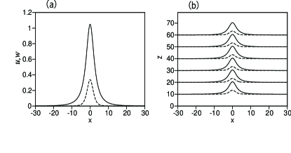
Figure 1: (a) Profiles $u(x)$ and $w(x)$ (solid and dashed lines, respectively) of the cross section, drawn through $y=0$, of the FF and SH components of the ground-state (zero-vorticity) stationary soliton solution of Eqs. (2) and (3) with LI $\alpha=1.5$, $k=0.0583$, and mismatch $Q=1$. It is tantamount to the solution of Eqs. (8) and (9) with the same parameters. The total power (10) of the soliton is $P=24.5$. (b) Snapshots of $|U(x)|$ and $|W(x)|$, taken at $z=10n$ ($n=1,2,\cdots,7)$, corroborate the stable evolution of this perturbed soliton.

In Fig. 2, families of fundamental solitons are characterized by the respective $P(k)$ dependences for two values of LI: an intermediate one, $\alpha=1.5$, and $\alpha=1.1$, which is close to the collapse threshold ($\alpha=1$), in terms of interval (4). The dependences are plotted for the three values of the mismatch, $Q=+1$, $0$, and $-1$, as fixed in Eq. (4). All the families are stable, in accordance with the fact that they satisfy the VK criterion, $dP/dk>0$, and in agreement with the well-known stability of the similar fundamental 2D solitons in the $\chi^{(2)}$ system with the normal (non-fractional) diffraction, $\alpha=2$. The dotted lines in Fig. 2(a) and (b) are $P=74.5k^{2/3}$ and $P=24.5k^{0.2/1.1}$, respectively, with the powers predicted by Eq. (14), and fitting numerical factors in front of the powers. These curves confirm the agreement of the numerical findings for $Q=0$ with the analytical prediction.

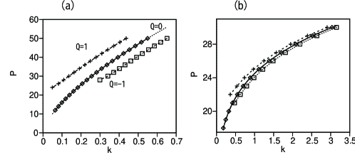
Figure 2: The relation between the total power (10) of stable fundamental solitons and their FF propagation constant $k$, at LI values $\alpha=1.5$ (a) and $\alpha=1.1$ (b), for the three fixed values of the mismatch, $Q=+1$ (crosses), $0$ (rhombuses), and $-1$ (squares), see Eq. (4).

Also in agreement with the analytical prediction for $Q=0$, the GS solitons exist and are stable at all values of $k$ (the same is found for other values of LI from interval (4)). On the other hand, for $Q=\pm 1$, the soliton solutions exist above the threshold (minimum) value of the power, $P\geq P_{\mathrm{thr}}$, and, accordingly, at $k\geq k_{\mathrm{thr}}$. The threshold power is plotted, as a function of LI, in Fig. 3. The comparison with the 1D version of the $\chi^{(2)}$ system, which was explored in Ref. [36], suggests that, at $Q=\pm 1$ and $k<k_{\mathrm{thr}}$, there should exist another, strongly unstable, branch of the soliton solutions (also taking values $P\geq P_{\mathrm{thr}}$), which merges with the stable one at $k=k_{\mathrm{thr}}$ and $P=P_{\mathrm{thr}}$. However, the IT simulations do not converge to strongly unstable solutions (in Ref. [36], the 1D unstable solutions were found by means of the Newton conjugate gradient method [47], which is not sensitive to the stability of the stationary solutions). On the other hand, at $P<P_{\mathrm{thr}}$ the IT simulations converge to a spatially uniform state .

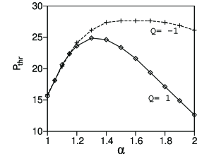
Figure 3: The threshold values of the power below which stable solitons do not exist at $Q=+1$ and $-1$( the solid and dashed lines, respectively).

The expected onset of the critical and supercritical collapse in the system of Eqs. (2) and (3) at $\alpha=1$ and $\alpha<1$, respectively, was also tested in direct simulations. As an example, Fig. 4 presents the findings for $\alpha=0.4$ (the deeply supercritical case) and $Q=0$, produced by inputs which were taken at $z=0$ as

$$U(x,y,0) = (1.21+0.88i)/\{9(x^{2}+y^{2})+1\},~{}W(x,y,0)=0;$$ (15)

$$U(x,y,0) = (0.99+0.72i)/\{9(x^{2}+y^{2})+1\},~{}W(x,y,0)=0.$$ (16)

Figure 4(a) shows that the former input gives rise to onset of the collapse through the steep growth of amplitude $\left|U\left(x=0,y=0,z\right)\right|$. On the other hand, input (16), with a somewhat smaller power, initiates the evolution which leads to the decay of the localized configuration (in the case which is generically categorized as the collapse, decay of particular inputs is possible too). The development of the collapse and decay, which are initiated, severally, by inputs (15) and (16) is directly illustrated by the evolution of the respective cross-section profiles in Figs. 4(b) and (c), respectively.

.

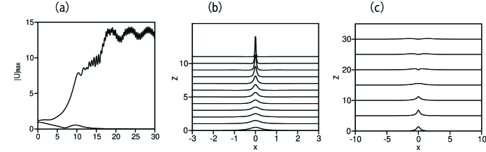
Figure 4: (a) The evolution of the FF amplitude, $|U(x=0,y=0,z)|$, as produced by simulations of Eqs. (2) and (3) with $\alpha=0.4$ and $Q=0$, and the initial conditions taken as per Eq. (15) (the collapsing solution) or Eq. (16) (the decaying one). (b) and (c): The corresponding evolution of the cross section of the FF profile, $|U(x,y=0,z)|$

III.2 Moving (tilted) solitons

The fractional diffraction operators destroy the Galilean invariance of Eqs. (2) and (3), therefore producing moving solitons (actually, ones tilted in the spatial domain) is a nontrivial problem. For this purpose, the underlying equation are rewritten in the tilted coordinates, with $x\rightarrow\tilde{x}\equiv x-vz$, where $v$ is the “velocity” (in fact, the tilt in the $\left(x,z\right)$ plane):

$$i\frac{\partial U}{\partial z}-iv\frac{\partial U}{\partial\tilde{x}} = \frac{1}{2}\left(-\frac{\partial^{2}}{\partial\tilde{x}^{2}}-\frac{\partial^{2}}{\partial y^{2}}\right)^{\alpha/2}U-WU^{\ast},$$ (17)

$$2i\frac{\partial W}{\partial z}-2iv\frac{\partial W}{\partial\tilde{x}} = \frac{1}{2}\left(-\frac{\partial^{2}}{\partial\tilde{x}^{2}}-\frac{\partial^{2}}{\partial y^{2}}\right)^{\alpha/2}W+QW-\frac{1}{2}U^{2}.$$ (18)

Stationary solutions for tilted solitons were produced by means of the IT algorithm applied to Eqs. (17) and (18), and their stability was again tested by simulations of the perturbed evolution in real time (real $z$, in fact). A typical family of stable soliton solutions is represented in Fig. 5(a) by the dependence of the FF amplitude, $U_{0}=\left|U\left(\tilde{x}=0,y=0\right)\right|$ vs. the tilt $v$ for a fixed value of the total power, $P=20$, setting $\alpha=1.5$ and $Q=0$ in Eqs. (17) and (18). It is seen that the solitons gradually shrink, increasing the amplitude, as $v$ grows from $0$ to $0.8$, and then rapidly expand, featuring steep fall of the amplitude. The soliton solution ceases to exist through delocalization at $v\approx 0.94$, when its amplitude vanishes. At $v>0.94$, the IT integration converges to a flat state. Figure 5(b) demonstrates an example of the stable soliton tilted with slope $v$ $=0.5$.

Of course, the solitons also exist with the opposite velocity (tilt), $-v,$ which makes it possible to simulate collisions between them. Figure 5(c) demonstrates that the collisions are fully inelastic, leading to mutual destruction of the solitons.

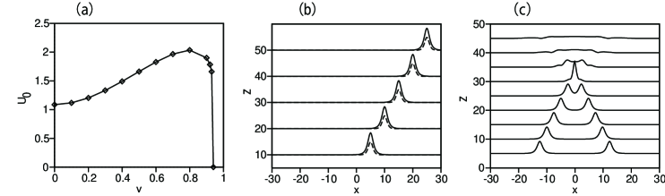
Figure 5: (a) The amplitude $U_{0}$ of the FF component of the “moving” (tilted) solitons with fixed power $P=20$ vs. the “velocity” $v$, as produced by the IT method applied to Eqs. (17) and (18) with $\alpha=1.5$, $Q=0$. (b) The evolution of $|U(x,z)|$ (the solid line) and $|W(x,z)|$ (the dashed line) for a stable “moving” (tilted) soliton with $v=0.5$, displayed in the cross section $y=0$. (c) The inelastic collision, leading to mutual destruction of the two moving solitons with $v=\pm 0.5$.

III.3 Unstable vortex solitons

As well as the usual $\chi^{(2)}$ system with the normal diffraction ($\alpha=2$), the present one, with LI $\alpha<2$, admits the existence of solitons with embedded vorticity, defined as per Eq. (11), with integer winding numbers $m$ and $2m$ in the phases of the FF and SH components, respectively. In particular, starting with the input $U\sim e^{i\theta}$ and $W\sim e^{2i\theta}$, the IT method, applied to Eqs. (2) and (3) with $\alpha=1.5$, produces a family of stationary soliton solutions in the form of vortex rings, with $m=1$ and powers $P\geq 111$ or $P\geq 139$ for $Q=+1$ and $-1$, respectively. These findings are illustrated, in Figs. 6(a) and 7(a), by plots of the cross sections of the FF and SH components of the vortex soliton (ring) for $P=150$ and mismatch parameters $Q=+1$ and $-1$, respectively.

Similar to the usual 2D $\chi^{(2)}$ solitons [41, 42], the ones produced by Eqs. (2) and (3) are subject to instability against spontaneous fission into fragments, which are close to individual stable fundamental solitons performing intrinsic vibrations, as shown in Figs. 6(c) and 7(c). The secondary solitons produced by the fission of the vortex ring are moving, to provide the conservation of the angular momentum (see Eq. (12)). It is seen that the fission leads to effective shrinkage of the fragments, in comparison to the original vortex ring. In  agreement with this observation, Figs. 6(b) and 7(b) demonstrate that, in the course of the fission, the amplitude (largest value of the FF component, $\left|U(x,y)\right|$) increases to values which are essentially higher than the initial one, and then performs residual oscillations. The latter feature implies that, as said above, the fundamental solitons are produced by the fission in an excited state (with internal vibrations). A similar fission of a vortex soliton into three fragments was observed at $\alpha=1.5$ and $P=140$ for $Q=0$.

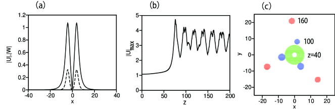
Figure 6: (a) Profiles of $|U(x)|$ and $|W(x)|$ in cross section $y=0$ for the vortex soliton with $m=1$ and power $P=130$, obtained as a stationary numerical solution for $\alpha=1.5$ and $Q=+1$ in Eqs. (8) and (9). (b) The maximum value of the FF component, $|U\left(x,y\right)|$, of the same soliton vs. propagation distance $z$, demonstrating the soliton’s instability. (c) For the same unstable soliton, the snapshots of the high-field regions, with $|U(x,y)|>0.5$, at $z=40$ (green), $100$ (blue), and $160$ (red), demonstrate that the original vortex ring spontaneously splits into the set of three moving fundamental (zero-vorticity) solitons in an excited state (with internal vibrations).

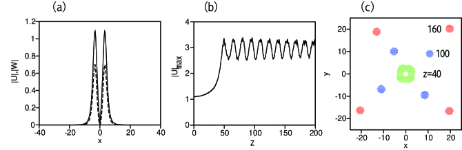
Figure 7: The same as in Fig. 6, but for the unstable vortex soliton with $P=150$, in the case of $Q=-1$. In this case, panel (c) demonstrates spontaneous fission into a set of four fundamental solitons in the excited form..

IV Solitons supported by the trapping potential and their stability

IV.1 Basic equations

The confining structure of the bulk waveguide may be represented by a trapping potential $V\left(x,y\right)$ added to Eqs. (2) and (3), which, in many cases, is taken in the isotropic quadratic form, $V(x,y)=V_{0}\left(x^{2}+y^{2}\right)$ with $V_{0}>0$ [48]. This modification of the $\chi^{(2)}$ system is relevant as the confining potential may help to stabilize solitons [43].

Thus, we now address the $\chi^{(2)}$ system with the quadratic potential:

$$i\frac{\partial U}{\partial z} = \frac{1}{2}\left(-\frac{\partial^{2}}{\partial x^{2}}-\frac{\partial^{2}}{\partial y^{2}}\right)^{\alpha/2}U-WU^{\ast}+\frac{1}{8}\left(x^{2}+y^{2}\right)U,$$ (19)

$$2i\frac{\partial W}{\partial z} = \frac{1}{2}\left(-\frac{\partial^{2}}{\partial x^{2}}-\frac{\partial^{2}}{\partial y^{2}}\right)^{\alpha/2}W+QW-\frac{1}{2}U^{2}+\frac{1}{2}\left(x^{2}+y^{2}\right)W.$$ (20)

Here, the coefficient in front of the potential term in Eq. (19) is fixed to be $1/8$ by means of scaling, and the fact that its counterpart in Eq. (20) is larger by the factor of $4$ is a generic feature of the $\chi^{(2)}$ system [35]. Stationary solutions of Eqs. (19) and (20) are looked for as per Eq. (7) with the FF propagation constant $k$, and functions $u$ and $w$ satisfying the equations

$$-ku = \frac{1}{2}\left(-\frac{\partial^{2}}{\partial x^{2}}-\frac{\partial^{2}}{\partial y^{2}}\right)^{\alpha/2}u-wu^{\ast}+\frac{1}{8}\left(x^{2}+y^{2}\right)u,$$ (21)

$$-4kw = \frac{1}{2}\left(-\frac{\partial^{2}}{\partial x^{2}}-\frac{\partial^{2}}{\partial y^{2}}\right)^{\alpha/2}w+Qw-\frac{1}{2}u^{2}+\frac{1}{2}\left(x^{2}+y^{2}\right)w.$$ (22)

IV.2 Soliton solutions

IV.2.1 Single-color states

First of all, Eqs. (19) and (20) admit obvious trapped SH-only (single-color) states with $U=0$, while $W$ is, obviously, tantamount to eigenstates of the linear fractional Schrödinger equation with the HO potential:

$$2i\frac{\partial W}{\partial z}=\frac{1}{2}\left(-\frac{\partial^{2}}{\partial x^{2}}-\frac{\partial^{2}}{\partial y^{2}}\right)^{\alpha/2}W+QW+\frac{1}{2}\left(x^{2}+y^{2}\right)W.$$ (23)

Stationary solutions to Eq. (23) are looked for in the usual form, $W\left(x,y,z\right)=e^{2ikz}w(x,y)$ (see Eq. (7)), with function $w(x,y)$ satisfying the equation

$$-4kw=\frac{1}{2}\left(-\frac{\partial^{2}}{\partial x^{2}}-\frac{\partial^{2}}{\partial y^{2}}\right)^{\alpha/2}w+Qw+\frac{1}{2}\left(x^{2}+y^{2}\right)w,$$ (24)

cf. Eq. (22).

The GS corresponds to the solution of Eq. (24) with zero SH vorticity, $m_{2}=0$, while $m_{2}=1,2,...$ correspond to excited states. In terms of the general form of the two-color vortex modes (11), we have $m_{2}\equiv 2m$, hence odd values of $m_{2}$ may represent solely single-color modes.

The single-color state in the finite-size system in the limit of vanishing LI, $\alpha\rightarrow 0$

First, we consider the case of $\alpha\rightarrow 0$. In terms of the split-step Fourier method implementing the numerical simulations, term $(-\partial^{2}/\partial x^{2}-\partial^{2}/\partial y^{2})^{\alpha/2}w$ in Eq. (24) is calculated by means of the Fourier transform as $\sum_{p_{x},p_{y}}(p_{x}^{2}+p_{y}^{2})^{\alpha/2}w_{p_{x},p_{y}}e^{ip_{x}x+ip_{y}y}$, where, in the limit if $\alpha\rightarrow 0$, we set $(p_{x}^{2}+p_{y}^{2})^{\alpha/2}=1$ for $p_{x}^{2}+p_{y}^{2}\neq 0$, and $(p_{x}^{2}+p_{y}^{2})^{\alpha/2}=0$ for $p_{x}=p_{y}=0$. Thus, because the dc (constant) Fourier component, corresponding to $p_{x}=p_{y}=0$, is eliminated, the spatial average of $(-\partial^{2}/\partial x^{2}-\partial^{2}/\partial y^{2})^{\alpha/2}w$ vanishes. Then, $w\left(x,y\right)$ is recovered by the inverse Fourier transform, with the first term on the right-hand side of Eq. (24) taking the form of

$$\frac{1}{2}w\left(x,y\right)-\frac{1}{2L^{2}}\int_{-L/2}^{+L/2}\int_{-L/2}^{+L/2}w\left(x^{\prime},y^{\prime}\right)dx^{\prime}dy^{\prime},$$ (25)

where $L\times L$ is the actual system’s size, and expression (25) secures the vanishing of the dc value, as said above.

In this case, we attempt to approximate the GS solution of Eq. (24) in the finite domain by a Lorentzian,

$$w=\frac{w_{0}}{1+\gamma(x^{2}+y^{2})}.$$ (26)

The substitution of this in Eq. (24) yields

$$\frac{-4kw_{0}}{1+\gamma(x^{2}+y^{2})}=\frac{1}{2}\left[\frac{w_{0}}{1+\gamma(x^{2}+y^{2})}-\bar{w}\right]+Q\frac{w_{0}}{1+\gamma(x^{2}+y^{2})}+\frac{x^{2}+y^{2}}{2}\frac{w_{0}}{1+\gamma(x^{2}+y^{2})},$$ (27)

where the spatial average $\bar{w}=(1/L^{2})\int\int w_{0}/\{1+\gamma(x^{2}+y^{2})\}dxdy$ in the finite domain is approximated as

$$\bar{w}=\frac{1}{L^{2}}\int_{0}^{L/2}\frac{w_{0}}{1+\gamma r^{2}}2\pi rdr=\frac{\pi w_{0}}{L^{2}\gamma}\ln\left[1+\gamma\left(\frac{L}{2}\right)^{2}\right].$$

From the comparison of the coefficients in  front of similar terms in Eq. (27), we obtain

$$\gamma=\frac{\exp\left(L^{2}/\pi\right)-1}{(L/2)^{2}},\;\bar{w}=\frac{\pi W_{0}\ln\left[1+\gamma(L/2)^{2}\right]}{\gamma L^{2}},\;k=(1/8)(\bar{w}-1)-\frac{Q}{4},$$ (28)

and amplitude $w_{0}$ of ansatz (26) is determined by the normalization condition,

$$\int\int w^{2}\left(x,y\right)dxdy\simeq\int_{0}^{L/2}\frac{w_{0}^{2}}{\left(1+\gamma r^{2}\right)^{2}}2\pi rdr=\frac{\pi\left(L/2\right)^{2}}{1+\gamma(L/2)^{2}}w_{0}^{2}=\frac{P}{4},$$

which yields

$$w_{0}=\frac{1}{L}\sqrt{\frac{P}{\pi}\left[1+\gamma(L/2)^{2}\right]}.$$ (29)

According to Eq. (28), width $1/\sqrt{\gamma}$ of Lorentzian (26) strongly (exponentially) depends on the system’s size $L$, due to the strong nonlocality of Eq. (24) in the limit of $\alpha\rightarrow 0$. For $L\rightarrow\infty$, the power density corresponding to the Lorentzian may be roughly approximated by the 2D delta-function:

$$4w^{2}(x,y)\simeq P\delta(x)\delta(y).$$

Figure 8 shows the cross sections, drawn through $y=0$, of the numerically found solution $w(x,y)$ (the solid line) for $P=4$, and of the corresponding approximate solution (26), with $\gamma=40.47$ and $W_{0}=3.60$, as given by Eqs. (28) and (29). It is seen that the Lorentzian ansatz yields an accurate approximation in this case.

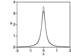
Figure 8: The profile of the GS single-color state $w$ produced by the linear Schrödinger equation Eq. (24) at $\alpha\rightarrow 0$ and $P=4$, in the domain of size $L\times L=4\times 4$. The solid line is the numerical result produced by the IT method, and the dashed line is the Lorentzian ansatz (26) with $\gamma=40.47$ and $w_{0}=3.60$, as given by Eqs. (28) and (29).

The single-color states with finite LI, $0<\alpha<2$

A nontrivial problem is the stability of the single-color solutions of the linear equation (24) against parametric excitations, i.e., small perturbations of the FF field $U$ driven by term $WU^{\ast}$ in Eq. (19). In the case of the non-fractional diffraction ($\alpha=2$), the parametric instability of such states, with $m_{2}=0$, $1$, and $2$, was investigated in Ref. [43]. It was found that the single-color states with each value of $m_{2}$ are stable for values of the power below a certain threshold,

$$P<\left(P_{\mathrm{thr}}\right)_{m}^{(\mathrm{single-color})},$$ (30)

which depends on the mismatch. At the threshold, the single-color states with even $m_{2}$ (actually, $m_{2}=0$ and $2$ were considered) underwent a pitchfork bifurcation [51], which gave rise to stable two-color states with FF vorticity $m_{2}/2$ at values of the power above the threshold. The single-color mode with $m_{2}=1$, which cannot bifurcate into a two-color vortex, was spontaneously transformed, above the threshold, into an apparently unstable state with chaotic oscillations.

For a crude estimate of the onset of the parametric instability of the single-color states, with $U=0$, we first analyze this issue in the case of the uniform state (in the absence of the trapping potential), which is represented by an evident solution of Eq. (3),

$$W(z)=W_{0}\exp\left(-iQz/2\right),$$ (31)

with a constant real amplitude $W_{0}$. Then, a small FF perturbation in substituted in Eq. (2) as $U\left(x,y,z\right)=U_{0}(z)\exp(ik_{x}x+ik_{y}y)$, with amplitude $U_{0}(z)$ satisfying the equation

$$i\frac{dU_{0}}{dz}=\frac{1}{2}k^{\alpha}U_{0}+W(z)U_{0},$$ (32)

where $k=\sqrt{k_{x}^{2}+k_{y}^{2}}$. Inserting $W(z)$ from Eq. (31) in Eq. (32), the ensuing solution for the FF perturbation amplitude is

$$U_{0}=U_{0}^{(0)}\exp\left[i\left(Q/4+i\lambda(k)\right)z\right],$$ (33)

with eigenvalue

$$\lambda(k)=\sqrt{\left(Q/4-k^{\alpha}\right)^{2}-W_{0}^{2}}.$$ (34)

For $Q=-1$, Eq. (33) yields real $\lambda$, i.e., stability, for all values of the perturbation wavenumber $k$, provided that the amplitude of the uniform SH state is small enough, $W_{0}<1/4$, irrespective of the LI value $\alpha$. Otherwise, as well as for all values of $W_{0}$ in the case of $Q=0$ and $Q=+1$, Eq. (34) yields imaginary $\lambda$, i.e., the parametric instability, at some values of $k$.

Proceeding to the single-color states trapped in the HO potential, which are produced as stationary solutions of the linear equation (23), examples of the GS with zero vorticity and excited state with vorticity $m_{2}=1$ are plotted, for LI values $\alpha=1.5$ and $0.5$, in Figs. 9(a) and 10(a), respectively. Here, $Q=-1$ is taken, as it facilitates the stability of the single-color states, pursuant to Eq. (34). The fractional diffraction is weaker for smaller LI $\alpha$, hence the respective profiles are sharper in Figs. 9(a) and 10(a).

The parametric (in)stability of the single-color ($W$-only) states was tested by seeding a perturbation in the $U$ component, with small amplitude $\varepsilon$ and the shape naturally chosen, at $z=0$, as

$$U_{m_{2}=0}^{(\mathrm{pert})}\left(x,y\right)=\varepsilon\exp\left(-r^{2}\right),U_{m_{2}=1}^{(\mathrm{pert})}\left(x,y\right)=\varepsilon\left(1+re^{i\theta}\right)\exp\left(-r^{2}\right),U_{m_{2}=2}^{(\mathrm{pert})}\left(x,y\right)=\varepsilon re^{i\theta}\exp\left(-r^{2}\right),$$ (35)

and running direct simulations of the perturbed evolution of the single-color states with the indicated values of the SH vorticity $m_{2}$. The results, which are displayed in Figs. 9(b,c) and 10(b,c) for $m_{2}=0$ (the GS) and $m_{2}=1$, respectively, demonstrate the existence of a critical (threshold) power of the single-color states, $\left(P_{\mathrm{thr}}\right)_{m_{2}}^{(\mathrm{single-color})}(\alpha)$ (cf. Eq. (30)), such that the single-color states are stable with the power below the critical value, and unstable above it. In particular, for the vortex states with $m_{2}=1$ the development of the instability is illustrated by the evolution of form-factors

$$S_{0}=\int\int\left|U\left(x,y\right)\right|dxdy,~{}S_{1}=\int\int\left|U\left(x,y.\right)e^{-i\theta}\right|dxdy.$$ (36)

The numerical findings yield the following values of the critical (threshold) power below which the single-color states keep their stability:

$$\left(P_{\mathrm{thr}}\right)_{m_{2}=0}^{(\mathrm{single-color})}\left(\alpha=0.1\right)\approx 0.35,~{}\left(P_{\mathrm{thr}}\right)_{m_{2}=0}^{(\mathrm{single-color})}\left(\alpha=0.5\right)\approx 3.5,~{}\left(P_{\mathrm{thr}}\right)_{m_{2}=0}^{(\mathrm{single-color})}\left(\alpha=1.5\right)\approx 9.3;$$

$$\left(P_{\mathrm{thr}}\right)_{m_{2}=1}^{(\mathrm{single-color})}\left(\alpha=0.5\right)\approx 5.9,~{}\left(P_{\mathrm{thr}}\right)_{m_{2}=1}^{(\mathrm{single-color})}\left(\alpha=1.5\right)\approx 18.6;$$

$$\left(P_{\mathrm{thr}}\right)_{m_{2}=2}^{(\mathrm{single-color})}\left(\alpha=0.5\right)\approx 7.55,~{}\left(P_{\mathrm{thr}}\right)_{m_{2}=2}^{(\mathrm{single-color})}\left(\alpha=1.5\right)\approx 23.9.$$ (37)

Note that the trapping potential makes it possible to create the stable single-color modes even at $\alpha\leq 1$, cf. the free-space stability interval (6). The threshold value increases with the increase of $\alpha$ (stronger diffraction, corresponding to larger $\alpha$, makes it easier to suppress the growth of small perturbations), and is larger for larger vorticity $m_{2}$.

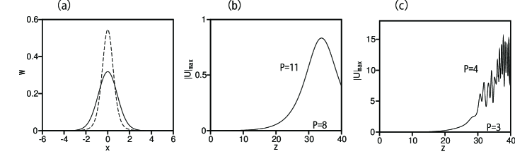
Figure 9: (a) Profiles of the trapped single-color GS, $w(x)$ (with $m_{2}=0$ and $P=1$), are shown in cross section $y=0$, as produced by the numerical IT solution of Eqs. (19) and (20) with $\alpha=1.5$ and $0.5$ (the solid and dashed lines, respectively). (b) The evolution of the amplitude, $|U(x=0)|$, for the same GS solutions with powers $P=8$ (stable) and $11$ (unstable), at $\alpha=1.5$. (c) The same as in (b), but for $P=3$ (stable) and $4$ (unstable) at $\alpha=0.5$. In all cases, $Q=-1$.

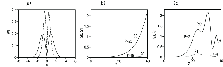
Figure 10: (a) Profiles of the trapped single-color state, $|W(x)|$. with vorticity $m_{2}=1$ and $P=1$ are shown in cross section $y=0$, as produced by the numerical solution of Eqs. (19) and (20) with $\alpha=1.5$ and $0.5$ (the solid and dashed lines, respectively). (b) The evolution of form-factors (36) for the vortex states with $m_{2}=1$ and powers $P=18$ (stable) and $20$ (unstable), the LI being $\alpha=1.5$. (c) The same as in (b), but for powers $P=5$ (stable) and $7$ (unstable), and LI $\alpha=0.5$.

IV.2.2 Two-color states

The destabilization of the single-color modes with $m_{2}=0$ and $2$ at the threshold points identified as per Eq. (37) is explained by a bifurcation which gives rise to two-color states, with $U\neq 0$. For the GS, with $m_{2}=0$, the transition from the single-color state to the two-color one, in the system with $Q=0$, is illustrated by panels (a) and (b) in Fig. 11. Systematically collected numerical results are presented in Fig. 11(c) as the chart in the (LI, power) plane, which includes areas populated by stable single- and two-color GSs, as well as the area (at larger $P$ and smaller $\alpha$) where the system blows up (the collapse takes place). We stress that the trapped GSs of both the single- and two-color types may be stable at $\alpha\leq 1$, while, as said above, all the stationary free-space states are unstable $\alpha\leq 1$. Note that the threshold value of the power at the single-color GS boundary is going to vanish, $\left(P_{\mathrm{thr}}\right)_{m_{2}=0}\rightarrow 0$ at $\alpha\rightarrow 0$. This feature complies with a very small value, $\left(P_{\mathrm{thr}}\right)_{m_{2}=0}^{(\mathrm{single-color})}\left(\alpha=0.1\right)\approx 0.35$ at small $\alpha=0.1$ and $Q=-1$ in Eq. (37) (which is different from $Q=0$ corresponding to Fig. 11(c)).

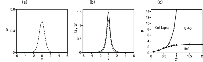
Figure 11: (a) The cross section of the stable single-color GS, represented solely by the SH component, $w$ (with $m_{2}=0$, and $U=0$), as produced by the IT method applied to Eqs. (19) and (20) for $\alpha=0.8$, $Q=0$, and $P=1.8$. (b) The stable two-color GS, which includes both the FF and SH compomnents ($u$ and $w$, respectively), obtained for $\alpha=0.8$, $Q=0$, and $P=4.5$. (c) The GS phase diagram in the parameter plane $\left(\alpha,P\right)$. Symbols $\mathrm{U=0}$ and $\mathrm{U}\mathrm{\neq 0}$ designate areas which are populated, respectively, by the stable single- and two-color GSs. In the limit of $\alpha=2$, the stability diagram carries over into the one known in the system with the normal (non-fractional) diffraction [43].

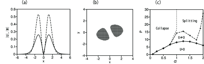
Figure 12: (a) A stable stationary two-color vortex state with $m_{2}=2$, as produced by the IT simulation method applied to Eqs. (19) and (20) with $\alpha=1.5$, $Q=0$, and power $P=10$. $|U|$ and $|W|$ are plotted by the solid and dashed lines, respectively. (b) A snapshot of the rotating pattern of $|U\left(x,y\right)|>0.5$ at $\alpha=1.5$, $Q=0$, and $P=24$, as produced by the spontaneous splitting (fission) of the unstable vortex state. (c) The stability diagram in the parameter plane of $\left(\alpha,P\right)$. Symbols $\mathrm{U=0}$ and $\mathrm{U}\mathrm{\neq 0}$ designate areas which are populated, respectively, by the stable single- and two-color vortex states. The splitting domain is populated by rotating dipoles, such as the one shown in panel (b). Similar to the situation plotted in Fig. 11, in the limit of $\alpha=2$, the stability diagram carries over into the one known in the system with the normal (non-fractional) diffraction [43].

A similar picture for the vortex states, with $m_{2}=2$, is presented in Fig. 12. Cross sections of the FF and SH components of a stable two-color state with $m_{1}=1$ and $m_{2}=2$ are plotted in Fig. 12(a) for $\alpha=1.5$, $Q=0$, and $P=10$ (examples of stable single-color vortex states with $m_{2}=2$ are not shown here). For $\alpha=1.5$ and $Q=0$, the vortex state with $m_{2}=2$ is unstable against spontaneous splitting in two fragments at $P>12.75$. Obeying the conservation of the angular momentum (see Eq. (12)), the fragments build a rotating dipole state, as shown in Fig. 12(b) for $P=24$. The angular velocity of the rotation of the emerging state is $\approx 0.34$.

Finally, the phase diagram for the vortex states is plotted in Fig. 12(c) in the plane of LI and power. Similar to the stability chart for the GS, displayed in Fig. 11(c), labels $\mathrm{U=0}$ and $\mathrm{U}\mathrm{\neq 0}$ designate parametric areas populated by the single- and two-color states, respectively. Unlike the GS chart, where the entire instability area is located, in Fig. 11(c), at $\alpha<1$ and, accordingly, represents the collapse, the instability area in Fig. 12(c) is separated by the vertical dashed line into the collapse domain at $\alpha<1$, and in the splitting one at $\alpha>1$.

V Conclusion

We have introduced the model for the spatial-domain copropagation of the FF (fundamental-frequency) and SH (second-harmonic) waves in the bulk waveguide with the $\chi^{(2)}$ nonlinearity and effective fractional transverse diffraction acting onto both components. The main objective of the analysis is to construct families of 2D fundamental (zero-vorticity) and vortical solitons and explore their stability. In the free-space system, we have obtained a family of stable fundamental solitons, in agreement with the VK (Vakhitov-Kolokolov) criterion, while all vortex solitons are unstable against spontaneous fission. Because the fractional diffraction breaks the system’s Galilean invariance, we have also produced solutions for moving stable fundamental solitons, and demonstrated that collisions between them are destructive.

Different results are produced for the FF-SH fractional $\chi^{(2)}$ system including the trapping HO (harmonic-oscillator) potential. The trap admits the existence of both single-color (SH-only) and two-color (FF-SH) solitons, including the fundamental ones and solitons carrying the embedded vorticity. The increase of the soliton’s power drives the bifurcation which transforms the single-color solitons into their two-color counterparts. The stability areas have been identified for the solitons of both types, with zero and nonzero vorticities alike.

As extension of the present analysis, it may be interesting to introduce the 2D three-wave system which, in terms of optics, corresponds to the copropagation of two different FF polarization components and the single SH wave, coupled by the $\chi^{(2)}$ interaction (the three-wave system is also known as the one realizing the Type-II $\chi^{(2)}$ interaction [35]). In that case, an additional control parameter is the birefringence of the FF components. The structure and stability of the solitons in the three-wave system may be essentially different.

References

- [1] M. Caputo, Linear model of dissipation whose Q is almost frequency independent. II, Geophysical Journal International 13, 529–539 (1967).
- [2] V. V. Uchaikin, Fractional Derivatives for Physicists and Engineers (Springer, New York, 2013).
- [3] N. Laskin, Fractional quantum mechanics, Phys. Rev. E 62, 3135-3145 (2000).
- [4] N. Laskin, Fractional quantum mechanics and Lévy path integrals, Phys. Lett. A 268, 298-305 (2000).
- [5] N. Laskin, Fractional quantum mechanics, World Scientific Publishing (Singapore, 2018).
- [6] S. Longhi, Fractional Schrödinger equation in optics, Opt Lett 40, 1117-1120 (2015).
- [7] S. Liu, Y. Zhang, B. A. Malomed, and E. Karimi, Experimental realisations of the fractional Schrödinger equation in the temporal domain, Nature Commun. 14, 222 (2023).
- [8] W. Zhong, M. R. Belić, and Y. Zhang, Accessible solitons of fractional dimension, Ann. Phys. 368, 110-116 (2016).
- [9] C. Huang and L. Dong, Gap solitons in the nonlinear fractional Schrödinger equation with an optical lattice. Opt. Lett. 41, 5636-5639 (2016).
- [10] J. Xiao, Z. Tian, C. Huang, and L. Dong, Surface gap solitons in a nonlinear fractional Schrödinger equation, Opt. Exp. 26, 2650-2658 (2018).
- [11] L. W. Zeng, M. R. Belić, D. Mihalache, J. Shi, J. Li, S. Li, X. Lu, Y. Cai , and J. Li, Families of gap solitons and their complexes in media with saturable nonlinearity and fractional diffraction, Nonlinear Dynamics 108, 671-680 (2022).
- [12] L. W. Zeng and J. H. Zeng, One-dimensional solitons in fractional Schrödinger equation with a spatially periodical modulated nonlinearity: nonlinear lattice, Opt. Lett. 44, 2661-2664 (2019).
- [13] M. I. Molina, The fractional discrete nonlinear Schrödinger equation, Phys. Lett. A 384, 126180 (2020).
- [14] M. N. Chen, Q. Guo, D. Q. Lu, and W. Hu, Variational approach for breathers in a nonlinear fractional Schrödinger equation, Commun. Nonlin. Sci. & Numer. Sim. 71, 73-81 (2019).
- [15] X. Yao and X. Liu, Off-site and on-site vortex solitons in space-fractional photonic lattices, Opt. Lett . 43, 5749-5752 (2018).
- [16] P. F. Li, B. A. Malomed, and D. Mihalache, Vortex solitons in fractional nonlinear Schrödinger equation with the cubic-quintic nonlinearity, Chaos Solitons & Fractals 137, 109783 (2020).
- [17] M. N. Chen, S. H. Zeng, D. Q. Lu, W. Hu, and Q. Guo, Optical solitons, self-focusing, and wave collapse in a space-fractional Schrödinger equation with a Kerr-type nonlinearity, Phys. Rev. E 98, 022211 (2018).
- [18] P. F. Li, B. A. Malomed, and D. Mihalache, Symmetry breaking of spatial Kerr solitons in fractional dimension, Chaos Solitons & Fractals 132, 109602 (2020).
- [19] J. B. Chen and J. H. Zeng, Spontaneous symmetry breaking in purely nonlinear fractional systems, Chaos 30, 063131 (2020).
- [20] L. W. Zeng and J. H. Zeng, Fractional quantum couplers, Chaos Solitons & Fractals 140, 110271 (2020).
- [21] S. Kumar, P. F. Li, and B. A. Malomed, Domain walls in fractional media, Phys. Rev. E 106, 054207 (2022).
- [22] D. V. Strunin and B. A. Malomed, Symmetry-breaking transitions in quiescent and moving solitons in fractional couplers, Phys. Rev. E 107, 064203 (2023).
- [23] L. W. Zeng, M. R. Belić, D. Mihalache, Q. Wang, J. B. Chen, J. C. Shi, Y. Cai, X. W. Lu, and J. Z. Li, Solitons in spin-orbit-coupled systems with fractional spatial derivatives, Chaos Solitons & Fractals 152, 111406 (2021).
- [24] H. Sakaguchi and B. A. Malomed, One- and two-dimensional solitons in spin-orbit-coupled Bose-Einstein condensates with fractional kinetic energy, J. Phys. B: At. Mol. Opt. Phys. 55, 155301 (2022).
- [25] W.-P. Zhong, M. R. Belić, B. A. Malomed, Y. Zhang, and T. Huang, Spatiotemporal accessible solitons in fractional dimensions, Phys. Rev. E 94, 012216 (2016).
- [26] W.-P. Zhong, M. Belić, and Y. Zhang, The fractional dimensional spatiotemporal accessible solitons supported by -symmetric complex potential, Annals of Physics (New York) 378, 432-439 (2017).
- [27] W.-P. Zhong, M. Belić, and Y. Zhang, Fraction-dimensional accessible solitons in a parity-time symmetric potential, Annalen der Physik (Berlin) 530, 1700311 (2018).
- [28] B. A. Malomed, Optical solitons and vortices in fractional media: A mini-review of recent results, Photonics 8, 353 (2021).
- [29] B. A. Malomed, Basic fractional nonlinear-wave models and solitons, Chaos 34, 022102 (2024).
- [30] B. A. Malomed, Fractional wave models and their experimental applications, in: Fractional Dispersive Models and Applications: Recent Developments and Future Perspectives, ed. by P. G. Kevrekidis and J. Cuevas-Maraver (Springer Nature Switzerland AG, Cham, 2024).
- [31] S. Liu, Y. Zhang, S. Virally, E. Karimi, B. A. Malomed, and D. V. Seletskiy, Observation of the spectral bifurcation in the fractional nonlinear Schrödinger equation, arXiv:2311.15150 (2023).
- [32] W. E. Torruellas, Z. Wang, D. J. Hagan, E. W. VanStryland, G. I. Stegeman, L. Torner, and C. R. Menyuk, Observation of two-dimensional spatial solitary waves in a quadratic medium, Phys. Rev. Lett. 74, 5036-5039 (1995).
- [33] G. I. Stegeman, D. J. Hagan, and L. Torner, cascading phenomena and their applications to all-optical signal processing, mode-locking, pulse compression and solitons, Opt. Quant. Elect. 28, 1691-1740 (1996).
- [34] C. Etrich, F. Lederer, B. A. Malomed, T. Peschel, and U. Peschel, Optical solitons in media with a quadratic nonlinearity, Prog. Opt. 41, 483-568 (2000).
- [35] A. V. Buryak, P. Di Trapani, D. V. Skryabin, and S. Trillo, Optical solitons due to quadratic nonlinearities: from basic physics to futuristic applications, Phys. Rep. 370, 63-235 (2002).
- [36] P. Li, H. Sakaguchi, L. Zeng, X. Zhu, D. Mihalache, and B. A. Malomed, Second-harmonic generation in the system with fractional diffraction, Chaos, Solitons & Fractals 173, 113701 (2023).
- [37] L. W. Zeng, Y. L. Zhu, B. A. Malomed, D. Mihalache, Q. Wang, H. Long, Y. Cai, X. W. Lu, and J. Z. Li, Quadratic fractional solitons, Chaos Solitons & Fractals 154, 111586 (2022).
- [38] D. S. Petrov and G. E. Astrakharchik, Ultradilute low-dimensional liquids. Phys. Rev. Lett. 117, 100401 (2016).
- [39] M. G. Vakhitov and A. A. Kolokolov, Stationary solutions of the wave equation in a medium with nonlinearity saturation, Radiophys Quantum Electron. 16, 7830789 (1973).
- [40] L, Bergé, Wave collapse in physics: principles and applications to light and plasma waves, Phys. Rep. 303, 259-370 (1998).
- [41] W. J. Firth and D. V. Skryabin, Phys. Rev. Letts. 79, 2450 (1997).
- [42] L. Torner and D. V. Petrov, Azimuthal instabilities and self-breaking of beams into sets of solitons in bulk second-harmonic generation, Electronics Lett. 33, 608-610 (1997).
- [43] H. Sakaguchi and B. A. Malomed, Stabilizing single- and two-color vortex beams in quadratic media by a trapping potential. J. Opt. Soc. Am. B 29, 2741-2748 (2012).
- [44] O. P. Agrawal, Fractional variational calculus in terms of Riesz fractional derivatives, J. Phys. A: Math. Theor. 40, 6287-6303 (2007).
- [45] M. Cai and C. P. Li, On Riesz derivative, Fractional Calculus and Applied Math. 22, 287-301 (2019).
- [46] W. Z. Bao and Q. Du, Computing the ground state solution of Bose-Einstein condensates by a normalized gradient flow, SIAM J. Sci. Comp. 25, 1674-1697 (2004).
- [47] J. K. Yang, Nonlinear Waves in Integrable and Nonintegrable Systems (SIAM. Philadelphia, 2010).
- [48] S. Raghavan and G. P. Agrawal, Spatiotemporal solitons in inhomogeneous nonlinear media, Opt. Commun. 180, 377-382 (2000).
- [49] H. Sakaguchi and B. A. Malomed, Solitons in combined linear and nonlinear lattice potentials, Phys. Rev. A 81, 013624 (2010).
- [50] L. P. Pitaevskii and S. Stringari, Bose-Einstein Condensation (Oxford University Press, Oxford, 2003).
- [51] G. Iooss and D. D. Joseph, Elementary Stability and Bifurcation Theory (Springer, New York, 1980).