Standard model of electromagnetism and chirality in crystals

R. Winkler Department of Physics, Northern Illinois University, DeKalb, IL 60115, USA Materials Science Division, Argonne National Laboratory, Argonne, Illinois 60439, USA    U. Zülicke MacDiarmid Institute, School of Chemical and Physical Sciences, Victoria University of Wellington, PO Box 600, Wellington 6140, New Zealand
(May 31, 2024)
Abstract

We present a general, systematic theory of electromagnetism and chirality in crystalline solids. Symmetry is its fundamental guiding principle. We use the formal similarity between space inversion $i$ and time inversion $\theta$ to identify two complementary, comprehensive classification of crystals, based on five categories of electric and magnetic multipole order—called polarizations—and five categories of chirality. The five categories of polarizations (parapolar, electropolar, magnetopolar, antimagnetopolar, and multipolar) expand the familiar notion of electric dipolarization in ferroelectrics and magnetization in ferromagnets to higher-order multipole densities. The five categories of chirality (parachiral, electrochiral, magnetochiral, antimagnetochiral, and multichiral) expand the familiar notion of enantiomorphism due to non-superposable mirror images to the inversion symmetries $i$, $\theta$, and $i\theta$. In multichiral systems, all these inversion symmetries are absent so that these systems have four distinct enantiomorphs. Each category of chirality arises from distinct superpositions of electric and magnetic multipole densities. We provide a complete theory of minimal effective models characterizing the different categories of chirality in different systems. Jointly these two schemes yield a classification of all 122 magnetic crystallographic point groups into 15 types that treat the inversion symmetries $i$, $\theta$, and $i\theta$ on the same footing. The group types are characterized via distinct physical properties and characteristic features in the electronic band structure. At the same time, the formal similarities between the inversion symmetries $i$, $\theta$, and $i\theta$ imply striking correspondences between apparently dissimilar systems and their physical properties.

I Introduction

Symmetry is a fundamental guiding principle in solid-state physics, linking the periodic crystal structure of solids with physical properties. Translational symmetry is usually the starting point for a discussion of crystal symmetries, it yields the well-known 14 Bravais lattices [1]. These get complemented by point-group symmetries, including space inversion $i$, to obtain the 230 crystallographic space groups [2]. In a last step, to account for magnetic phenomena, one may incorporate time inversion $\theta$ to construct the 1651 magnetic space groups [3].

Important progress in our understanding of the physical properties of crystalline solids was made early on with Neumann’s principle [4, 5] stating that macroscopic properties of a crystal structure do not require a knowledge of the space group characterizing a crystal structure. Instead, these properties are already determined by the simpler crystallographic point groups that include proper and improper rotations as its group elements, but no translations [6, 7, 2, 8, 3].

The present work goes one step beyond Neumann’s principle by taking space inversion symmetry (SIS) and time inversion symmetry (TIS) as its starting point. SIS and TIS are among the most fundamental symmetries describing the universe. Both SIS and TIS are so-called black-white symmetries; they are represented by two-element groups $C_{i}=\{e,i\}$ and $C_{\theta}=\{e,\theta\}$ that are obviously isomorphic [9]. (Here $e$ denotes the unit element.) This formal similarity between SIS and TIS allows us to develop a unified treatment of these symmetries, where we identify $i$ and $\theta$ as duals of each other. The relationship of duality allows one to classify magnetic point groups such that $i$ and $\theta$ are treated on an equal footing. In the present work, we follow Neumann’s principle by not considering translational symmetries.

Here we are particularly interested in electric and magnetic multipole order in solids. This fundamental property of solids is characterized by spontaneously formed order/̄$\ell$ multipole densities, which we call polarizations. Examples include the electric dipolarization ($\ell=1$) in ferroelectrics and the magnetization in ferromagnets. Whereas multipole densities in crystals defy a naive definition using classical electromagnetism [10, 11, 12], group theory expanding on Neumann’s principle provides a precise formalism for discussing electric and magnetic multipole order in solids. Early studies identified crystal structures permitting a bulk electric dipolarization [4, 5, 13] or a bulk magnetization [14, 15, 16]. More recent work focused on higher-order multipole densities [17, 18, 19, 20, 21, 22]. Some work also studied electrotoroidal [23, 24] and magnetotoroidal [25] multipole densities, though their physical significance has remained unclear [26]. We show how toroidal multipole densities arise as compound multipole densities. The treatment of multipole densities as strictly macroscopic quantities distinguishes our theory from other work [18, 19, 20, 21].

Table 1: Signature $ss^{\prime}$ of multipoles of order $\ell$. Respective columns define the electric, magnetic, and toroidal IRs $D_{\ell}^{ss^{\prime}}$ and irreducible spherical tensors $T_{\ell}^{ss^{\prime}}$ of the full rotation group $R_{i\times\theta}$.
electric magnetic electro- toroidal magneto- toroidal
$\ell$ even $++$ $--$ $-+$ $+-$
$\ell$ odd $-+$ $+-$ $++$ $--$

Following Ref. [22], we identify four types of polarizations—electric, magnetic, electrotoroidal, and magnetotoroidal, see Table 1. The signature $ss^{\prime}$ indicates how a polarization behaves under space inversion (even/odd if $s=+/-$) and time inversion (even/odd if $s^{\prime}=+/-$). Odd/̄$\ell$ electric (signature $-+$) and odd/̄$\ell$ magnetic ($+-$) multipole densities are duals of each other, whereas even/̄$\ell$ electric ($++$) and even/̄$\ell$ magnetic ($--$) multipole densities are self-dual.

The set of 122 crystallographic magnetic point groups and the range of physical properties they represent reveal a yet deeper structure beyond SIS-TIS duality when space inversion $i$ and time inversion $\theta$ are combined in the full inversion group $C_{i\times\theta}=\{e,i,\theta,i\theta\}$ that is isomorphic to Klein’s four group in abstract group theory [3]. This group treats the three elements $\gamma=i$ (SIS), $\theta$ (TIS), and $i\theta$ (combined inversion symmetry, CIS) on an equal footing. The inversion symmetries $\gamma$ allow us to define two complementary, comprehensive classifications of crystals, using five categories of polarizations and five categories of chirality. Both schemes classify the electric and magnetic order in crystal structures based on the presence or absence of the inversion symmetries $\gamma$, but from rather different perspectives.

In each scheme, the five categories stand for the five subgroups of the group $C_{i\times\theta}$. The five categories of polarizations reflect the presence or absence of the inversion symmetries $\gamma$ as independent elements in the symmetry group $G$ of a physical system [22]. In the parapolar category, all three inversion symmetries $\gamma$ represent good symmetries so that only even/̄$\ell$ electric multipole densities called parapolarizations are allowed. These even/̄$\ell$ multipole densities are also allowed in all other categories. For the three unipolar categories, only one of the symmetries $\gamma$ represents a good symmetry. In the electropolar category, TIS is a good symmetry that permits odd/̄$\ell$ electric multipole densities called electropolarizations. In the magnetopolar category, SIS is a good symmetry that permits odd/̄$\ell$ magnetic multipole densities called magnetopolarizations. In the antimagnetopolar category, CIS is a good symmetry that permits even/̄$\ell$ magnetic multipole densities called antimagnetopolarizations. Finally, in the multipolar category, all three symmetries $\gamma$ are broken so that all four types of polarizations may coexist. Each category of polarizations gives rise to distinctive indicators in the electronic band structure [22].

Denoting proper rotations by $C$, the five categories of chirality, on the other hand, reflect the presence or absence in $G$ of any composite symmetry elements $\gamma C$, i.e., presence or absence of $\gamma$/̄improper rotations. Systems whose symmetries include $i$/̄improper and $\theta$/̄improper (and thus also $i\theta$/̄improper) rotations are parachiral and show no enantiomorphism. Each of the three unichiral categories includes $\gamma$/̄improper rotations for only one inversion symmetry $\gamma$. Systems with only $\theta$/̄improper rotations among its symmetries are electrochiral and exist in two enantiomorphic versions that are transformed into each other by $i$/̄improper and $i\theta$/̄improper rotations. In addition to this conventional case [27], we identify the categories of magnetochiral systems (having only $i$/̄improper rotations) and antimagnetochiral systems (having only $i\theta$/̄improper rotations). Each of these categories permits two enantiomorphs. The two enantiomorphs of magnetochiral systems are superposed by $\theta$/̄improper and $i\theta$/̄improper rotations, whereas $\theta$/̄improper and $i$/̄improper rotations transform between the two enantiomorphs of antimagnetochiral systems. In addition, systems whose only symmetries are proper rotations (none of them combined with $i$, $\theta$ or $i\theta$) are multichiral and exist in four distinct enantiomorphs.

We show how each category of chirality arises from distinct superpositions of electric and magnetic multipole densities. Also, we discuss band-structure indicators of chirality. For this, we provide a complete theory of minimal effective models characterizing the different categories of chirality in different systems. These minimal models demonstrate explicitly how chirality in crystalline solids requires the interplay of multiple terms, either the interplay of unipolar and parapolar terms, or the interplay of multiple unipolar terms. Chirality in infinite crystal structures is qualitatively different from chirality in finite molecules.

Studying the morphology of the 122 magnetic point groups has been essential for gaining a basic understanding of general materials properties [28, 29, 30, 31, 32, 33, 34, 35, 36, 37]. Our systematic approach reveals fundamental patterns in the structure of magnetic point groups and the composition of Laue classes assembled by these. We identify 15 group types, where each type is characterized by a distinct combination of a category of polarizations and a category of chirality that act jointly like a unique identifier for each group type. These group types provide a comprehensive, fine-grained classification of all 122 magnetic crystallographic point groups and of the physical properties the groups imply.

Group theory provides yet deeper insights. For example, the group morphology becomes remarkably similar for each of the three unipolar categories electropolar, magnetopolar, and antimagnetopolar and for each of the three unichiral categories electrochiral, magnetochiral, and antimagnetochiral. The groups in these categories can thus be combined in triadic relations that imply striking correspondences between apparently dissimilar systems and their physical properties. We illustrate this point by tabulating the form of material tensors for all magnetic point groups.

Motivated by the completeness of our classification scheme and the comprehensive range of physical insights emerging from our theory, we call this approach the standard model of electromagnetism and chirality in crystals. It is equally applicable to insulators and metals, and it reveals fundamental connections between crystal structure and physical properties of solids. Our work systematizes, simplifies and greatly extends earlier studies [29, 30, 31, 32, 33, 34, 35, 36, 38, 39]. It is useful in the general context of understanding hidden orders in solids [40] and to inform the design of experimental probes [41].

The remainder of this article is organized as follows. We start by elucidating the general composition of magnetic point groups in Sec. II. The classification of continuous and discrete magnetic point groups is discussed in Sec. III. Section IV focuses on the description of electric and magnetic multipole order in solids. Our theory of chirality in solids is developed in in Sec. V. Each main section has a preamble that introduces the topics discussed later on. Conclusions and a brief outlook are presented in Sec. VI. Appendix A reviews the general group-theoretical framework underlying the refined symmetry classifications used in this work, with Appendix A.2 commenting briefly on spin groups. The concept of subclasses of magnetic point groups is introduced in Sec. II.5. Appendix B provides further details about the form of subclasses $L(G_{0}^{i\theta},i\theta)$. Appendix C presents a detailed discussion of the irreducible representations of the continuous axial groups that we refer to repeatedly in this work. Appendix D includes a tabulation of spherical tensors and multipole order permitted by the 122 crystallographic magnetic point groups. The commonalities regarding the shape of tensors implied by symmetry is elucidated in Appendix E. Finally, Appendix F tabulates materials candidates for the different categories of chirality introduced in Sec. V.

II Composition of magnetic point groups

The symmetry of a crystal structure is fully characterized by its (magnetic) space group $S$, which includes point symmetries, translations, and combinations thereof [2]. However, according to Neumann’s principle [4, 5, 8], macroscopic properties of a crystal structure such as material tensors and electric and magnetic polarization densities that may be realized in a structure depend only on the magnetic point group $G$ associated with the space group $S$. We therefore focus on point groups $G$ in this work. For crystal structures transforming according to a symmorphic space group $S_{\mathrm{s}}$, the point group $G$ is the finite subgroup of $S_{\mathrm{s}}$ consisting of the elements of $S_{\mathrm{s}}$ that leave one point in space fixed. Nonsymmorphic space groups $S_{\mathrm{n}}$ also contain group elements that combine point-group symmetries $g$ with nonprimitive translations. Here the elements $g$ are also elements of the point group $G$, although these symmetry operations are not, by themselves, elements of $S_{\mathrm{n}}$. The latter case makes crystallographic point groups defining crystal classes qualitatively distinct from point groups of finite systems like molecules.

This section reviews the basic structure and properties of magnetic point groups and introduces a new classification scheme where SIS and TIS are systematically treated on the same footing. The relationships revealed through this classification underpin our subsequent comprehensive discussion of multipole order in crystals (Sec. IV) and extensions to the concept of chirality (Sec. V). Throughout this work, we adhere to the Schönflies notation to denote symmetry elements and symmetry groups [42].

II.1 Black-white symmetries and inversion groups

Rotation symmetries are represented by proper point groups $G_{\mathrm{p}}$ that only contain proper rotations as symmetry elements. In contrast, SIS and TIS are both examples of so-called black-white symmetries [43, 3, 44], which are represented by two-element groups of the form

$$C_{\gamma}=\{e,\gamma\}\quad.$$ (1)

Here $e$ is the identity, and $\gamma$ is the single nontrivial group element that transforms between two qualities, represented abstractly by “black” and “white”, satisfying $\gamma^{2}=e$. Space inversion $i$ is such an operation, as is time inversion $\theta$ (for our systems of interest [9]), and their combination $i\theta$ (CIS). We use the symbols $C_{i}$, $C_{\theta}$, and $C_{i\theta}$ to refer to the inversion groups $C_{\gamma}$ defined in Eq. (1) when $\gamma=i$, $\theta$, and $i\theta$, respectively. For completeness and notational simplicity, we also define the full inversion group $C_{i\times\theta}\equiv C_{i}\times C_{\theta}=\{e,i,\theta,i\theta\}$ and the trivial inversion group $C_{1}=\{e\}$. In the following, the symbol $C_{\zeta}$ stands for any of the five inversion groups $C_{i\times\theta}$, $C_{\theta}$, $C_{i}$, $C_{i\theta}$, or $C_{1}$.

II.2 Combining a black-white symmetry with other symmetries

There are three possible types of point groups $G$ that arise from the combination of a black-white symmetry $\gamma$ with other symmetries. These types are conventionally labelled [43, 3] as colorless, major and minor groups, respectively. As we consider multiple black-white symmetries in this work, we make their definitions more specific:

  1. (a)

    The $\gamma$colorless groups $G^{(\mathrm{a})}$ do not contain $\gamma$ at all.

  2. (b)

    The $\gamma$major groups are of the form

    $$G^{(\mathrm{b})}=G^{(\mathrm{a})}\times C_{\gamma}\quad.$$ (2)
  3. (c)

    Suppose a $\gamma$/̄colorless group $G^{(\mathrm{a})}$ contains an invariant subgroup of index 2 denoted $\tilde{G}^{(\mathrm{a})}$, i.e.,

    $$G^{(\mathrm{a})}=\tilde{G}^{(\mathrm{a})}+\bar{g}\,\tilde{G}^{(\mathrm{a})}\quad,$$ (3a)
    where $\bar{g}\in G^{(\mathrm{a})}$, but $\bar{g}\notin\tilde{G}^{(\mathrm{a})}$. Then, the $\gamma$minor group is defined as
    $$G^{(\mathrm{c})}\equiv G^{(\mathrm{a})}\langle\tilde{G}^{(\mathrm{a})}\rangle_{\gamma}=\tilde{G}^{(\mathrm{a})}+\gamma\bar{g}\,\tilde{G}^{(\mathrm{a})}\quad.$$ (3b)

By definition, the major group $G^{(\mathrm{a})}\times C_{\gamma}$ contains the colorless group $G^{(\mathrm{a})}$ and the minor groups $G^{(\mathrm{a})}\langle\tilde{G}^{(\mathrm{a})}\rangle_{\gamma}$ as subgroups;

$\displaystyle G^{(\mathrm{a})}$ $\displaystyle\subset G^{(\mathrm{a})}\times C_{\gamma}\,\,,$ (4a)
$\displaystyle G^{(\mathrm{a})}\langle\tilde{G}^{(\mathrm{a})}\rangle_{\gamma}$ $\displaystyle\subset G^{(\mathrm{a})}\times C_{\gamma}\,\,.$ (4b)

We adopt the convention established in the context of incorporating TIS, whereby, for $\gamma=\theta$, the resulting groups $G^{(\mathrm{a})}$, $G^{(\mathrm{b})}$ and $G^{(\mathrm{c})}$ have been referred to as type I, type II and type III, respectively [43, 45], with the particular type/̄III notation

$$\gamma=\theta:\qquad G(\tilde{G})\equiv G\langle\tilde{G}\rangle_{\theta}\quad.$$ (5a)
Similarly, we label groups $G^{(\mathrm{a})}$, $G^{(\mathrm{b})}$ and $G^{(\mathrm{c})}$ arising in the process of incorporating SIS, i.e., when $\gamma=i$, as type i, type ii and type iii, respectively, and denote type/̄iii groups by
$$\gamma=i:\qquad G[\tilde{G}]\equiv G\langle\tilde{G}\rangle_{i}\quad.$$ (5b)
Groups that contain both $i$ and $\theta$ can also be classified as major or minor groups with respect to $i\theta$. We make use of this possibility later on, indicating $i\theta$/̄minor groups by
$$\gamma=i\theta:\qquad G\{\tilde{G}\}\equiv G\langle\tilde{G}\rangle_{i\theta}\quad.$$ (5c)

II.3 Classes and types of magnetic point groups; duality

Proper point groups $G_{\mathrm{p}}$ are both $i$/̄colorless and $\theta$/̄colorless, and thus also $i\theta$/̄colorless. Combining these with SIS using the formalism described in Sec II.2 yields the ordinary improper point groups [6, 3] that can be either $i$/̄major or $i$/̄minor. These groups are still $\theta$/̄colorless and $i\theta$/̄colorless. Combining these groups with TIS in the same way yields the magnetic point groups. In this process of extending the proper point groups by adding SIS and TIS, each proper point group $G_{\mathrm{p}}$ spawns a class $L(G_{\mathrm{p}})$ of magnetic point groups $G$ [32, 33, 34, 35] defined via

$$L(G_{\mathrm{p}})=\{G:G\mapsto G_{\mathrm{p}}\;\mbox{when}\;i,\theta\mapsto e\}\;.$$ (6)

By definition, each magnetic point group $G$ belongs to one and only one class $L(G_{\mathrm{p}})$. We call the proper point group $G_{\mathrm{p}}$ the class root of the class $L(G_{\mathrm{p}})$.

Table 2: Classification of magnetic point groups based on the SIS-TIS duality relation (7). We give the general form of each type and specify the number of groups of a given type among the 122 crystallographic magnetic point groups. Duality-related types are positioned underneath the self-dual type with which they form a triad. In addition to the short type label, we provide a full label indicating the types with respect to SIS (i, ii or iii), TIS (I, II or III) and CIS (J, JJ or JJJ). Small $2\times 2$ matrices mark congruences between tensors with signature $ss^{\prime}$ as discussed in detail in Appendix E. The categories of multipole order (i.e., polarization) and chirality are listed for each type. Notation: $G_{\mathrm{p}}$ denotes a proper point group, $\tilde{G}_{\mathrm{p}}$ is an index/̄2 subgroup of $G_{\mathrm{p}}$, superscripts $(j)$ distinguish distinct index/̄2 subgroups of $G_{\mathrm{p}}$, unprimed and primed groups denote versions of the same index/̄2 subgroup of $G_{\mathrm{p}}$ distinguished by different orientations of the coordinate system defining the group elements, and the inversion groups $C_{\zeta}$ are defined in Sec. II.1. See also Fig. 1.
self-dual type J $\equiv$ i-I-J ii/̄II $\equiv$ ii-II-JJ JJJ” $\equiv$ iii’-III’-JJJ’
general form $G_{\mathrm{p}}$ $G_{\mathrm{p}}\times C_{i\times\theta}$ $\begin{array}[]{nccln}&G_{\mathrm{p}}\{\tilde{G}_{\mathrm{p}}\}\,(\tilde{G}_{\mathrm{p}}^{\prime}\{\accentset{\approx}{G}_{\mathrm{p}}\})&=G_{\mathrm{p}}\{\tilde{G}_{\mathrm{p}}^{\prime\prime}\}\,[\tilde{G}_{\mathrm{p}}^{\prime}\{\accentset{\approx}{G}_{\mathrm{p}}\}]\\ =&G_{\mathrm{p}}(\tilde{G}_{\mathrm{p}}^{\prime})\,\{\tilde{G}_{\mathrm{p}}(\accentset{\approx}{G}_{\mathrm{p}})\}&=G_{\mathrm{p}}[\tilde{G}_{\mathrm{p}}^{\prime}]\,\{\tilde{G}_{\mathrm{p}}^{\prime\prime}[\accentset{\approx}{G}_{\mathrm{p}}]\}\\ =&G_{\mathrm{p}}[\tilde{G}_{\mathrm{p}}]\,(\tilde{G}_{\mathrm{p}}^{\prime\prime}[\accentset{\approx}{G}_{\mathrm{p}}])&=G_{\mathrm{p}}(\tilde{G}_{\mathrm{p}}^{\prime\prime})\,[\tilde{G}_{\mathrm{p}}(\accentset{\approx}{G}_{\mathrm{p}})]\end{array}$
allowed tensors (𝕏𝕏𝕏𝕏𝕏𝕏𝕏𝕏\begin{array}[]{@{}>{\scriptstyle}cs{0.08em}>{\scriptstyle}c@{}}\mcirc\hfil\hskip 0.56001pt&\mcirc\\[-6.88889pt] \mcirc\hfil\hskip 0.56001pt&\mcirc\end{array}) (𝕏   𝕏   \begin{array}[]{@{}>{\scriptstyle}cs{0.08em}>{\scriptstyle}c@{}}\mcirc\hfil\hskip 0.56001pt&\rule{3.01389pt}{0.0pt}\\[-6.88889pt] \rule{3.01389pt}{0.0pt}\hfil\hskip 0.56001pt&\rule{3.01389pt}{0.0pt}\end{array}) (𝕏𝕏missing-subexpression\begin{array}[]{@{}>{\scriptstyle}cs{0.08em}>{\scriptstyle}c@{}}\mcirc\hfil\hskip 0.56001pt&\mstar\scriptstyle\hfil\\[-6.88889pt] \mstar\scriptstyle\hfil\hfil\hskip 0.56001pt&\mstar\scriptstyle\hfil\end{array})
polarization multipolar parapolar multipolar
chirality multichiral parachiral parachiral
number of groups 11 11 1
self-dual type JJ $\equiv$ i-I-JJ JJ’ $\equiv$ iii-III-JJ JJJ $\equiv$ i-I-JJJ
general form $G_{\mathrm{p}}\times C_{i\theta}$ $G_{\mathrm{p}}[\tilde{G}_{\mathrm{p}}]\times C_{i\theta}=G_{\mathrm{p}}(\tilde{G}_{\mathrm{p}})\times C_{i\theta}$ $G_{\mathrm{p}}\{\tilde{G}_{\mathrm{p}}\}$
allowed tensors (𝕏  𝕏𝕏  𝕏\begin{array}[]{@{}>{\scriptstyle}cs{0.08em}>{\scriptstyle}c@{}}\mcirc\hfil\hskip 0.56001pt&\rule{3.01389pt}{0.0pt}\\[-6.88889pt] \rule{3.01389pt}{0.0pt}\hfil\hskip 0.56001pt&\mcirc\end{array}) (𝕏  𝕏  missing-subexpression\begin{array}[]{@{}>{\scriptstyle}cs{0.08em}>{\scriptstyle}c@{}}\mcirc\hfil\hskip 0.56001pt&\rule{3.01389pt}{0.0pt}\\[-6.88889pt] \rule{3.01389pt}{0.0pt}\hfil\hskip 0.56001pt&\mstar\scriptstyle\hfil\end{array}) (𝕏𝕏𝕏missing-subexpressionmissing-subexpression𝕏\begin{array}[]{@{}>{\scriptstyle}cs{0.08em}>{\scriptstyle}c@{}}\mcirc\hfil\hskip 0.56001pt&\mstar\scriptstyle\hfil\\[-6.88889pt] \mstar\scriptstyle\hfil\hfil\hskip 0.56001pt&\mcirc\end{array})
polarization antimagnetopolar antimagnetopolar multipolar
chirality antimagnetochiral parachiral antimagnetochiral
number of groups 11 10 10
dual types i-II-J $\equiv$ i/̄II  $\leftrightarrow$  ii/̄I $\equiv$ ii-I-J iii-II-JJJ $\equiv$ iii/̄II  $\leftrightarrow$  ii/̄III $\equiv$ ii-III-JJJ i-III-J $\equiv$ i/̄III  $\leftrightarrow$  iii/̄I $\equiv$ iii-I-J
general form $G_{\mathrm{p}}\times C_{\theta}$  $\leftrightarrow$  $G_{\mathrm{p}}\times C_{i}$ $\begin{array}[]{rln}&G_{\mathrm{p}}[\tilde{G}_{\mathrm{p}}]\times C_{\theta}\\ =&G_{\mathrm{p}}\{\tilde{G}_{\mathrm{p}}\}\times C_{\theta}\end{array}\bigg{\}}\!$  $\leftrightarrow$  $\!\bigg{\{}\begin{array}[]{rl}&G_{\mathrm{p}}(\tilde{G}_{\mathrm{p}})\times C_{i}\\ =&G_{\mathrm{p}}\{\tilde{G}_{\mathrm{p}}\}\times C_{i}\end{array}$ $G_{\mathrm{p}}(\tilde{G}_{\mathrm{p}})$  $\leftrightarrow$  $G_{\mathrm{p}}[\tilde{G}_{\mathrm{p}}]$
allowed tensors (𝕏 𝕏 𝕏 𝕏 \begin{array}[]{@{}>{\scriptstyle}cs{0.08em}>{\scriptstyle}c@{}}\mcirc\hfil\hskip 0.56001pt&\rule{3.01389pt}{0.0pt}\\[-6.88889pt] \mcirc\hfil\hskip 0.56001pt&\rule{3.01389pt}{0.0pt}\end{array})  $\leftrightarrow$  (𝕏𝕏  𝕏𝕏  \begin{array}[]{@{}>{\scriptstyle}cs{0.08em}>{\scriptstyle}c@{}}\mcirc\hfil\hskip 0.56001pt&\mcirc\\[-6.88889pt] \rule{3.01389pt}{0.0pt}\hfil\hskip 0.56001pt&\rule{3.01389pt}{0.0pt}\end{array}) (𝕏  𝕏 missing-subexpression \begin{array}[]{@{}>{\scriptstyle}cs{0.08em}>{\scriptstyle}c@{}}\mcirc\hfil\hskip 0.56001pt&\rule{3.01389pt}{0.0pt}\\[-6.88889pt] \mstar\scriptstyle\hfil\hfil\hskip 0.56001pt&\rule{3.01389pt}{0.0pt}\end{array})  $\leftrightarrow$  (𝕏  𝕏missing-subexpression  \begin{array}[]{@{}>{\scriptstyle}cs{0.08em}>{\scriptstyle}c@{}}\mcirc\hfil\hskip 0.56001pt&\mstar\scriptstyle\hfil\\[-6.88889pt] \rule{3.01389pt}{0.0pt}\hfil\hskip 0.56001pt&\rule{3.01389pt}{0.0pt}\end{array}) (𝕏𝕏𝕏missing-subexpression𝕏missing-subexpression\begin{array}[]{@{}>{\scriptstyle}cs{0.08em}>{\scriptstyle}c@{}}\mcirc\hfil\hskip 0.56001pt&\mstar\scriptstyle\hfil\\[-6.88889pt] \mcirc\hfil\hskip 0.56001pt&\mstar\scriptstyle\hfil\end{array})  $\leftrightarrow$  (𝕏𝕏𝕏𝕏\begin{array}[]{@{}>{\scriptstyle}cs{0.08em}>{\scriptstyle}c@{}}\mcirc\hfil\hskip 0.56001pt&\mcirc\\[-6.88889pt] \mstar\scriptstyle\hfil\hfil\hskip 0.56001pt&\mstar\scriptstyle\hfil\end{array})
polarization electropolar  $\leftrightarrow$  magnetopolar electropolar  $\leftrightarrow$  magnetopolar multipolar  $\leftrightarrow$  multipolar
chirality electrochiral  $\leftrightarrow$  magnetochiral parachiral  $\leftrightarrow$  parachiral electrochiral  $\leftrightarrow$  magnetochiral
number of groups 11  $\leftrightarrow$  11 10  $\leftrightarrow$  10 10  $\leftrightarrow$  10
self-dual type JJJ’ $\equiv$ iii-III-JJJ’
general form $\begin{array}[]{ccl}&G_{\mathrm{p}}\{\tilde{G}_{\mathrm{p}}^{(1)}\}\,(\tilde{G}_{\mathrm{p}}^{(2)}\{\accentset{\approx}{G}_{\mathrm{p}}\})&=G_{\mathrm{p}}\{\tilde{G}_{\mathrm{p}}^{(1^{\prime})}\}\,[\tilde{G}_{\mathrm{p}}^{(2)}\{\accentset{\approx}{G}_{\mathrm{p}}\}]\\ =&G_{\mathrm{p}}(\tilde{G}_{\mathrm{p}}^{(2)})\,\{\tilde{G}_{\mathrm{p}}^{(1)}(\accentset{\approx}{G}_{\mathrm{p}})\}&=G_{\mathrm{p}}[\tilde{G}_{\mathrm{p}}^{(2)}]\,\{\tilde{G}_{\mathrm{p}}^{(1^{\prime})}[\accentset{\approx}{G}_{\mathrm{p}}]\}\\ =&G_{\mathrm{p}}[\tilde{G}_{\mathrm{p}}^{(1)}]\,(\tilde{G}_{\mathrm{p}}^{(1^{\prime})}[\accentset{\approx}{G}_{\mathrm{p}}])&=G_{\mathrm{p}}(\tilde{G}_{\mathrm{p}}^{(1^{\prime})})\,[\tilde{G}_{\mathrm{p}}^{(1)}(\accentset{\approx}{G}_{\mathrm{p}})]\end{array}$
allowed tensors (𝕏𝕝𝕝𝕏𝕝𝕝missing-subexpression\begin{array}[]{@{}>{\scriptstyle}cs{0.08em}>{\scriptstyle}c@{}}\mcirc\hfil\hskip 0.56001pt&\mdiamond\\[-6.88889pt] \mdiamond\hfil\hskip 0.56001pt&\mstar\scriptstyle\hfil\end{array})
polarization multipolar
chirality parachiral
number of groups 2
dual types iii’-III-JJJ $\equiv$ iii’/̄III  $\leftrightarrow$  iii/̄III’ $\equiv$ iii-III’-JJJ
general form $\left.\begin{array}[]{ccl}&G_{\mathrm{p}}(\tilde{G}_{\mathrm{p}}^{(1)})\,[\tilde{G}_{\mathrm{p}}^{(2)}(\accentset{\approx}{G}_{\mathrm{p}})]&=G_{\mathrm{p}}(\tilde{G}_{\mathrm{p}}^{(1^{\prime})})\,\{\tilde{G}_{\mathrm{p}}^{(2)}(\accentset{\approx}{G}_{\mathrm{p}})\}\\ =&G_{\mathrm{p}}[\tilde{G}_{\mathrm{p}}^{(2)}]\,(\tilde{G}_{\mathrm{p}}^{(1)}[\accentset{\approx}{G}_{\mathrm{p}}])&=G_{\mathrm{p}}\{\tilde{G}_{\mathrm{p}}^{(2)}\}\,(\tilde{G}_{\mathrm{p}}^{(1^{\prime})}\{\accentset{\approx}{G}_{\mathrm{p}}\})\\ =&G_{\mathrm{p}}\{\tilde{G}_{\mathrm{p}}^{(1)}\}\,[\tilde{G}_{\mathrm{p}}^{(1^{\prime})}\{\accentset{\approx}{G}_{\mathrm{p}}\}]&=G_{\mathrm{p}}[\tilde{G}_{\mathrm{p}}^{(1^{\prime})}]\,\{\tilde{G}_{\mathrm{p}}^{(1)}[\accentset{\approx}{G}_{\mathrm{p}}]\}\end{array}\right\}$  $\leftrightarrow$  $\left\{\begin{array}[]{ccl}&G_{\mathrm{p}}[\tilde{G}_{\mathrm{p}}^{(1)}]\,(\tilde{G}_{\mathrm{p}}^{(2)}[\accentset{\approx}{G}_{\mathrm{p}}])&=G_{\mathrm{p}}[\tilde{G}_{\mathrm{p}}^{(1^{\prime})}]\,\{\tilde{G}_{\mathrm{p}}^{(2)}[\accentset{\approx}{G}_{\mathrm{p}}]\}\\ =&G_{\mathrm{p}}(\tilde{G}_{\mathrm{p}}^{(2)})\,[\tilde{G}_{\mathrm{p}}^{(1)}(\accentset{\approx}{G}_{\mathrm{p}})]&=G_{\mathrm{p}}\{\tilde{G}_{\mathrm{p}}^{(2)}\}\,[\tilde{G}_{\mathrm{p}}^{(1^{\prime})}\{\accentset{\approx}{G}_{\mathrm{p}}\}]\\ =&G_{\mathrm{p}}\{\tilde{G}_{\mathrm{p}}^{(1)}\}\,(\tilde{G}_{\mathrm{p}}^{(1^{\prime})}\{\accentset{\approx}{G}_{\mathrm{p}}\})&=G_{\mathrm{p}}(\tilde{G}_{\mathrm{p}}^{(1^{\prime})})\,\{\tilde{G}_{\mathrm{p}}^{(1)}(\accentset{\approx}{G}_{\mathrm{p}})\}\end{array}\right.$
allowed tensors (𝕏𝕝𝕝𝕏𝕝missing-subexpression𝕝\begin{array}[]{@{}>{\scriptstyle}cs{0.08em}>{\scriptstyle}c@{}}\mcirc\hfil\hskip 0.56001pt&\mdiamond\\[-6.88889pt] \mstar\scriptstyle\hfil\hfil\hskip 0.56001pt&\mdiamond\end{array})  $\leftrightarrow$  (𝕏𝕝𝕝𝕏missing-subexpression𝕝𝕝\begin{array}[]{@{}>{\scriptstyle}cs{0.08em}>{\scriptstyle}c@{}}\mcirc\hfil\hskip 0.56001pt&\mstar\scriptstyle\hfil\\[-6.88889pt] \mdiamond\hfil\hskip 0.56001pt&\mdiamond\end{array})
polarization multipolar  $\leftrightarrow$  multipolar
chirality parachiral  $\leftrightarrow$  parachiral
number of groups 2  $\leftrightarrow$  2
Refer to caption
Figure 1: Subgroup relations and isomorphisms between groups in a given class $L(G_{\mathrm{p}})$. Subgroup relations are depicted by lines. Groups placed within the same row are isomorphic. The categories of polarization and chirality for each group are also indicated, with the prefix “uni” representing “electro”, “magneto”, or “antimagneto”. Numbers $n$ at the lower right of a box specify how many groups represented by a box can be realized for inversion symmetries $\gamma,\bar{\gamma}=i$, $\theta$, and $i\theta$ with $\bar{\gamma}\neq\gamma$. When $n=1$, these groups are self-triadic. When $n=3$, these groups form a triad [Eq. (10)]. When a line connects groups that depend on $\gamma,\bar{\gamma}$, the subgroup relation exists pairwise between the groups in the triads with the same $\gamma,\bar{\gamma}$. Every class $L(G_{\mathrm{p}})$ contains the groups shown in the left (dark-blue) column. If $G_{\mathrm{p}}$ has an index/̄2 subgroup $\tilde{G}_{\mathrm{p}}$, the class also includes the groups in the center (medium-blue) column. If $\tilde{G}_{\mathrm{p}}$ has an index/̄2 subgroup $\accentset{\approx}{G}_{\mathrm{p}}$, the class also includes the groups in the right (light-blue) column. Below the dividing line at the bottom, subgroup relations between groups in the class $L(G_{\mathrm{p}})$ and the groups $\tilde{G}_{\mathrm{p}}$ and $\accentset{\approx}{G}_{\mathrm{p}}$ are shown. See also Table 2 that presents the groups that may exist in a class $L(G_{\mathrm{p}})$ in a more fine-grained way by indicating their types.

The separate consideration of the two black-white properties $i$ and $\theta$ yields overlapping group types, i.e., the full set of magnetic point groups can be viewed in terms of TIS as a collection of types I, II and III, or seen equivalently [30, 31] in terms of SIS as a collection of types i, ii and iii. Yet another classification can be based on CIS. We now develop a scheme that treats SIS and TIS symmetrically and makes CIS explicit, thus providing a systematic and complete classification of the magnetic point groups. This approach also reveals a general structure underlying the composition of the class $L(G_{\mathrm{p}})$ of magnetic point groups with class root $G_{\mathrm{p}}$.

It has previously been observed [30] that exchanging $i\leftrightarrow\theta$ in all group elements of a magnetic point group $G$ yields another magnetic point group $G_{\mathrm{d}}$. Clearly, the groups $G$ and $G_{\mathrm{d}}$ are isomorphic. We call this relationship SIS-TIS duality or $i\leftrightarrow\theta$ duality

$$G\;\leftrightarrow\;G_{\mathrm{d}}$$ (7)

with dual partners $G$ and $G_{\mathrm{d}}$. It is easy to see that dual partners $G$ and $G_{\mathrm{d}}$ belong to the same class $L(G_{\mathrm{p}})$, i.e., both $G$ and $G_{\mathrm{d}}$ satisfy Eq. (6) with the same class root $G_{\mathrm{p}}$. The concept of duality allows one to classify the groups in a given class $L(G_{\mathrm{p}})$ as follows.

Self-dual groups $G=G_{\mathrm{d}}\in L(G_{\mathrm{p}})$ are invariant under exchange $i\leftrightarrow\theta$. They belong to one (and only one) of the seven types LABEL:gcat:J, LABEL:gcat:ii-II, LABEL:gcat:JJ, LABEL:gcat:JJp, LABEL:gcat:JJJ, LABEL:gcat:JJJp, or LABEL:gcat:JJJpp defined in Table 2. Besides the self-dual types, we have types associated with dual pairs $G\;\leftrightarrow\;G_{\mathrm{d}}$ with $G\neq G_{\mathrm{d}}$ and $G,G_{\mathrm{d}}\in L(G_{\mathrm{p}})$. We label these types by indicating their respective types under both SIS and TIS. See Table 2 for the explicit definitions. In the following, we generally use short labels when referring to one of the new types, but an instructive full label indicating their types under SIS, TIS and CIS is also given in Table 2.

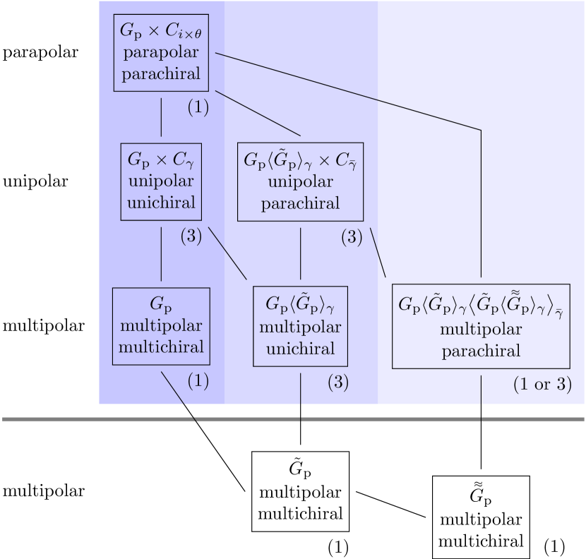
Within each class, the groups of the types LABEL:gcat:J, LABEL:gcat:JJJ, LABEL:gcat:JJJp, LABEL:gcat:JJJpp, LABEL:gcat:i-III, LABEL:gcat:iii-I, LABEL:gcat:iiip-III, and LABEL:gcat:iii-IIIp are all isomorphic. Furthermore, the groups of the types LABEL:gcat:JJ, LABEL:gcat:JJp, LABEL:gcat:i-II, LABEL:gcat:ii-I, LABEL:gcat:ii-III, and LABEL:gcat:iii-II are all isomorphic. A group of type LABEL:gcat:ii-II is not isomorphic to any other group in the same class but contains all of these as its subgroups. See Fig. 1 for a description of general isomorphisms and subgroup relations between magnetic-point-group types in a given class. Isomorphisms formed the basis of a prior classification scheme of the 122 magnetic crystallographic groups [32, 33].

Table 2 provides comprehensive information about the 15 magnetic-point-group types, including associated categories of multipole order and chirality. These properties are further elucidated in Secs. IV and V.

The present classification treats $\theta$ as a black-white symmetry like $i$ so that $\theta^{2}=e$. This is the case for systems with integer spin angular momentum (the single groups), and it is relevant for all macroscopic properties of a crystal structure such as those characterized by Neumann’s principle [4, 5]. The isomorphisms discussed here do not hold for the respective double groups characterizing half-integer-spin degrees of freedom [9].

Table 3: Subclasses $L(G_{0}^{\gamma},\gamma)$ and groups in a class $L(G_{\mathrm{p}})$. The groups in $L(G_{\mathrm{p}})$ are arranged in the upper part of the table according to the scheme shown in the center part of the table, where each group’s type as well as its categories of polarization and chirality are indicated. Here $\tilde{G}_{\mathrm{p}}$ denotes an index/̄2 subgroup of the class root $G_{\mathrm{p}}$. For clarity, we omit multipolar-parachiral groups of type LABEL:gcat:JJJpp, LABEL:gcat:JJJp, LABEL:gcat:iiip-III, and LABEL:gcat:iii-IIIp. The subclass $L(G_{0}^{\theta},\theta)$ for each group is specified in the header of its column. For groups of type LABEL:gcat:JJ or LABEL:gcat:JJp, their subclass $L(G_{0}^{i},i)$ is also given in the column header. Groups of all other types have their subclass $L(G_{0}^{i},i)$ specified in the header of their respective row. Small $2\times 2$ matrices mark congruences between tensors with signature $ss^{\prime}$ as discussed in detail in Appendix E. The bottom part of the table lists the groups in the subclasses $L(G_{0}^{i\theta},i\theta)\equiv L(G_{0\mathrm{d}}^{i\theta},i\theta)$.
$L(G_{0}^{i},i)\,\backslash\,L(G_{0}^{\theta},\theta)$ $L(G_{\mathrm{p}},\theta)$ $L(G_{\mathrm{p}}[\tilde{G}_{\mathrm{p}}],\theta)$ $L(G_{\mathrm{p}}\times C_{i},\theta)$ $L(G_{\mathrm{p}}\times C_{i},\theta),$ $L(G_{\mathrm{p}}\times C_{\theta},i)$
L(Gp,i)𝐿subscript𝐺p𝑖\rule{0.0pt}{12.05553pt}L(G_{\mathrm{p}},i) Gpsubscript𝐺pG_{\mathrm{p}} (𝕏𝕏𝕏𝕏)𝕏𝕏𝕏𝕏(\raisebox{0.86108pt}[0.0pt][0.0pt]{$\begin{array}[]{@{}>{\scriptstyle}cs{0.08em}>{\scriptstyle}c@{}}\mcirc\hfil\hskip 0.56001pt&\mcirc\\[-6.88889pt] \mcirc\hfil\hskip 0.56001pt&\mcirc\end{array}$}) Gp[G~p]subscript𝐺pdelimited-[]subscript~𝐺pG_{\mathrm{p}}[\tilde{G}_{\mathrm{p}}] (𝕏𝕏)𝕏𝕏(\raisebox{0.86108pt}[0.0pt][0.0pt]{$\begin{array}[]{@{}>{\scriptstyle}cs{0.08em}>{\scriptstyle}c@{}}\mcirc\hfil\hskip 0.56001pt&\mcirc\\[-6.88889pt] \mstar\scriptstyle\hfil\hfil\hskip 0.56001pt&\mstar\scriptstyle\hfil\end{array}$}) Gp×Cisubscript𝐺psubscript𝐶𝑖G_{\mathrm{p}}\times C_{i} (𝕏𝕏  )𝕏𝕏  (\raisebox{0.86108pt}[0.0pt][0.0pt]{$\begin{array}[]{@{}>{\scriptstyle}cs{0.08em}>{\scriptstyle}c@{}}\mcirc\hfil\hskip 0.56001pt&\mcirc\\[-6.88889pt] \rule{3.01389pt}{0.0pt}\hfil\hskip 0.56001pt&\rule{3.01389pt}{0.0pt}\end{array}$}) Gp×Ciθsubscript𝐺psubscript𝐶𝑖𝜃G_{\mathrm{p}}\times C_{i\theta} (𝕏  𝕏)𝕏  𝕏(\raisebox{0.86108pt}[0.0pt][0.0pt]{$\begin{array}[]{@{}>{\scriptstyle}cs{0.08em}>{\scriptstyle}c@{}}\mcirc\hfil\hskip 0.56001pt&\rule{3.01389pt}{0.0pt}\\[-6.88889pt] \rule{3.01389pt}{0.0pt}\hfil\hskip 0.56001pt&\mcirc\end{array}$})
L(Gp(G~p),i)𝐿subscript𝐺psubscript~𝐺p𝑖L(G_{\mathrm{p}}(\tilde{G}_{\mathrm{p}}),i) Gp(G~p)subscript𝐺psubscript~𝐺pG_{\mathrm{p}}(\tilde{G}_{\mathrm{p}}) (𝕏𝕏)𝕏missing-subexpression𝕏missing-subexpression(\raisebox{0.86108pt}[0.0pt][0.0pt]{$\begin{array}[]{@{}>{\scriptstyle}cs{0.08em}>{\scriptstyle}c@{}}\mcirc\hfil\hskip 0.56001pt&\mstar\scriptstyle\hfil\\[-6.88889pt] \mcirc\hfil\hskip 0.56001pt&\mstar\scriptstyle\hfil\end{array}$}) Gp{G~p}subscript𝐺psubscript~𝐺pG_{\mathrm{p}}\{\tilde{G}_{\mathrm{p}}\} (𝕏𝕏)𝕏missing-subexpressionmissing-subexpression𝕏(\raisebox{0.86108pt}[0.0pt][0.0pt]{$\begin{array}[]{@{}>{\scriptstyle}cs{0.08em}>{\scriptstyle}c@{}}\mcirc\hfil\hskip 0.56001pt&\mstar\scriptstyle\hfil\\[-6.88889pt] \mstar\scriptstyle\hfil\hfil\hskip 0.56001pt&\mcirc\end{array}$}) Gp(G~p)×Cisubscript𝐺psubscript~𝐺psubscript𝐶𝑖G_{\mathrm{p}}(\tilde{G}_{\mathrm{p}})\times C_{i} (𝕏  )𝕏missing-subexpression  (\raisebox{0.86108pt}[0.0pt][0.0pt]{$\begin{array}[]{@{}>{\scriptstyle}cs{0.08em}>{\scriptstyle}c@{}}\mcirc\hfil\hskip 0.56001pt&\mstar\scriptstyle\hfil\\[-6.88889pt] \rule{3.01389pt}{0.0pt}\hfil\hskip 0.56001pt&\rule{3.01389pt}{0.0pt}\end{array}$}) Gp(G~p)×Ciθsubscript𝐺psubscript~𝐺psubscript𝐶𝑖𝜃G_{\mathrm{p}}(\tilde{G}_{\mathrm{p}})\times C_{i\theta} (𝕏  )𝕏  missing-subexpression(\raisebox{0.86108pt}[0.0pt][0.0pt]{$\begin{array}[]{@{}>{\scriptstyle}cs{0.08em}>{\scriptstyle}c@{}}\mcirc\hfil\hskip 0.56001pt&\rule{3.01389pt}{0.0pt}\\[-6.88889pt] \rule{3.01389pt}{0.0pt}\hfil\hskip 0.56001pt&\mstar\scriptstyle\hfil\end{array}$})
L(Gp×Cθ,i)𝐿subscript𝐺psubscript𝐶𝜃𝑖L(G_{\mathrm{p}}\times C_{\theta},i) Gp×Cθsubscript𝐺psubscript𝐶𝜃G_{\mathrm{p}}\times C_{\theta} (𝕏 𝕏 )𝕏 𝕏 (\raisebox{0.86108pt}[0.0pt][0.0pt]{$\begin{array}[]{@{}>{\scriptstyle}cs{0.08em}>{\scriptstyle}c@{}}\mcirc\hfil\hskip 0.56001pt&\rule{3.01389pt}{0.0pt}\\[-6.88889pt] \mcirc\hfil\hskip 0.56001pt&\rule{3.01389pt}{0.0pt}\end{array}$}) Gp[G~p]×Cθsubscript𝐺pdelimited-[]subscript~𝐺psubscript𝐶𝜃G_{\mathrm{p}}[\tilde{G}_{\mathrm{p}}]\times C_{\theta} (𝕏  )𝕏 missing-subexpression (\raisebox{0.86108pt}[0.0pt][0.0pt]{$\begin{array}[]{@{}>{\scriptstyle}cs{0.08em}>{\scriptstyle}c@{}}\mcirc\hfil\hskip 0.56001pt&\rule{3.01389pt}{0.0pt}\\[-6.88889pt] \mstar\scriptstyle\hfil\hfil\hskip 0.56001pt&\rule{3.01389pt}{0.0pt}\end{array}$}) Gp×Ci×θsubscript𝐺psubscript𝐶𝑖𝜃G_{\mathrm{p}}\times C_{i\times\theta} (𝕏   )𝕏   (\raisebox{0.86108pt}[0.0pt][0.0pt]{$\begin{array}[]{@{}>{\scriptstyle}cs{0.08em}>{\scriptstyle}c@{}}\mcirc\hfil\hskip 0.56001pt&\rule{3.01389pt}{0.0pt}\\[-6.88889pt] \rule{3.01389pt}{0.0pt}\hfil\hskip 0.56001pt&\rule{3.01389pt}{0.0pt}\end{array}$})
LABEL:gcat:J   multipolar multichiral LABEL:gcat:iii-I   multipolar magnetochiral LABEL:gcat:ii-I   magnetopolar magnetochiral LABEL:gcat:JJ antimagnetopolar antimagnetochiral
LABEL:gcat:i-III   multipolar electrochiral LABEL:gcat:JJJ   multipolar antimagnetochiral LABEL:gcat:ii-III   magnetopolar parachiral LABEL:gcat:JJp antimagnetopolar parachiral
LABEL:gcat:i-II   electropolar electrochiral LABEL:gcat:iii-II   electropolar parachiral LABEL:gcat:ii-II   parapolar parachiral
$\rule{0.0pt}{12.91663pt}\makebox[160.00024pt][l]{$L(G_{\mathrm{p}},i\theta)$}G_{\mathrm{p}},\;G_{\mathrm{p}}\{\tilde{G}_{\mathrm{p}}\},\;G_{\mathrm{p}}\times C_{i\theta}$
$\makebox[160.00024pt][l]{$L(G_{\mathrm{p}}(\tilde{G}_{\mathrm{p}}),i\theta)\,\,\equiv L(G_{\mathrm{p}}[\tilde{G}_{\mathrm{p}}],i\theta)$}G_{\mathrm{p}}(\tilde{G}_{\mathrm{p}}),\;G_{\mathrm{p}}[\tilde{G}_{\mathrm{p}}],\;G_{\mathrm{p}}(\tilde{G}_{\mathrm{p}})\times C_{i\theta}\equiv G_{\mathrm{p}}[\tilde{G}_{\mathrm{p}}]\times C_{i\theta}$
$\makebox[160.00024pt][l]{$L(G_{\mathrm{p}}\times C_{\theta},i\theta)\equiv L(G_{\mathrm{p}}\times C_{i},i\theta)$}G_{\mathrm{p}}\times C_{\theta},\;G_{\mathrm{p}}\times C_{i},\;G_{\mathrm{p}}\times C_{i\times\theta},\;G_{\mathrm{p}}[\tilde{G}_{\mathrm{p}}]\times C_{\theta},\;G_{\mathrm{p}}(\tilde{G}_{\mathrm{p}})\times C_{i}$

II.4 Triadic relationships

The SIS-TIS duality (7) appears naturally when magnetic point groups are constructed in the usual way from proper point groups by adding the black-white symmetries space inversion $i$ and time inversion $\theta$ [6, 14] as reviewed at the beginning of Sec. II.3. (See also Appendix A.) The duality (7) turns out to be useful to discuss physical phenomena involving electric and magnetic fields, and we make extensive use of it in the remainder of this work. Before delving onto these applications of SIS-TIS duality, we briefly discuss the deeper mathematical structure from which the duality emerges.

The full inversion group $C_{i\times\theta}$ has order 4. It is isomorphic to the Klein four-group

$$K_{4}=\{e,\gamma^{\prime},\gamma^{\prime\prime},\tilde{\gamma}=\gamma^{\prime}\gamma^{\prime\prime}:\gamma^{\prime\,2}=\gamma^{\prime\prime\,2}=\tilde{\gamma}^{2}=e\}$$ (8)

in abstract group theory [3]. This group treats the elements $\gamma^{\prime},\gamma^{\prime\prime}$, and $\tilde{\gamma}=\gamma^{\prime}\gamma^{\prime\prime}$ fully symmetrically. Indeed, one can express the full inversion group $C_{i\times\theta}$ in three equivalent forms

$$C_{i\times\theta}=C_{i}\times C_{\theta}\equiv C_{\theta}\times C_{i\theta}\equiv C_{i\theta}\times C_{i}\,\,.$$ (9)

Starting from a proper point group $G_{\mathrm{p}}$, it is thus possible to construct all magnetic point groups in the class $L(G_{\mathrm{p}})$ using any pair of inversion symmetries $\gamma^{\prime},\gamma^{\prime\prime}\in\{i,\theta,i\theta\}$ by first adding the black-white symmetry $\gamma^{\prime}$ and then adding $\gamma^{\prime\prime}$. Therefore, the concept of duality exists for any pair of inversion symmetries $\gamma^{\prime},\gamma^{\prime\prime}\in\{i,\theta,i\theta\}$. The resulting dualities are represented by the diagram

$G_{\theta}$ $G_{i}$ $G_{i\theta}$ $\theta\;\leftrightarrow\;i$

$i\theta\;\leftrightarrow\;i$

$\theta\;\leftrightarrow\;i\theta$

(10)

with triadic partners $G_{i}$, $G_{\theta}$, and $G_{i\theta}$ that are pairwise connected by duality relations similar to Eq. (7).

Triadic partners $G_{i}$, $G_{\theta}$, and $G_{i\theta}$ are isomorphic. A set of triadic partners $G_{i}$, $G_{\theta}$, and $G_{i\theta}$ constitutes a triad of magnetic groups. Possibilities for forming triads are shown in Table 2. Self-triadic groups are invariant under all dualities in the diagram (10). They belong to the types LABEL:gcat:J, LABEL:gcat:ii-II, or LABEL:gcat:JJJpp. The remaining groups form triads with distinct partners $G_{i}$, $G_{\theta}$, and $G_{i\theta}$ as indicated in Table 2. The index $\tilde{\gamma}=\gamma^{\prime}\gamma^{\prime\prime}$ of a group $G_{\tilde{\gamma}}$ in the diagram (10) indicates self-duality under the exchange $\gamma^{\prime}\leftrightarrow\gamma^{\prime\prime}$. The equivalent expressions provided in Table 2 for groups LABEL:gcat:JJJpp, LABEL:gcat:iii-II, LABEL:gcat:ii-III, LABEL:gcat:JJp, LABEL:gcat:iiip-III, LABEL:gcat:iii-IIIp, and LABEL:gcat:JJJp, emphasize the respective self-dualities of these groups.

II.5 Subclasses of magnetic point groups

In later sections, we want to classify the tensors permitted by the different groups $G$ in a class $L(G_{\mathrm{p}})$. For this purpose, the concept of subclasses of magnetic point groups turns out to be useful. For $\gamma=i$, $\theta$, and $i\theta$, the subclasses $L(G_{0}^{\gamma},\gamma)$ of a class $L(G_{\mathrm{p}})$ are the subsets of groups $G$

$$L(G_{0}^{\gamma},\gamma)=\{G:G\mapsto G_{0}^{\gamma}\;\mbox{when}\;\gamma\mapsto e\}\;.$$ (11)

For given $\gamma$, the subclasses $L(G_{0}^{\gamma},\gamma)$ of $L(G_{\mathrm{p}})$ are disjoint, i.e., each group $G\in L(G_{\mathrm{p}})$ belongs to one subclass $L(G_{0}^{i},i)$, one subclass $L(G_{0}^{\theta},\theta)$, and one subclass $L(G_{0}^{i\theta},i\theta)$. The subclasses derived for $\gamma=i$, $\theta$, and $i\theta$ hence represent alternative schemes for partitioning $L(G_{\mathrm{p}})$. Conversely, for a given class $L(G_{\mathrm{p}})$ and fixed $\gamma=i$, $\theta$, or $i\theta$, the subclasses $L(G_{0}^{\gamma},\gamma)$ spawn the class $L(G_{\mathrm{p}})$, i.e.,

$$L(G_{\mathrm{p}})=\bigcup_{G_{0}^{\gamma}}L(G_{0}^{\gamma},\gamma)\quad\mbox{for fixed $\gamma=i$, $\theta$ or $i\theta$.}$$ (12)

The subclass root $G_{0}^{\gamma}$ of the subclass $L(G_{0}^{\gamma},\gamma)$ is $\gamma$/̄colorless by construction. If $G_{0}^{\gamma}=G_{\mathrm{p}}$ the subclass root $G_{0}^{\gamma}$ is entirely colorless. The associated subclasses $L(G_{\mathrm{p}},\gamma)$ for $\gamma=i$, $\theta$, and $i\theta$ comprise $G_{\mathrm{p}}$, $G_{\mathrm{p}}\times C_{\gamma}$ and all $\gamma$/̄minor groups $G_{\mathrm{p}}\langle\tilde{G}_{\mathrm{p}}\rangle_{\gamma}$.

If the subclass root $G_{0}^{\gamma}$ still contains another black-white symmetry, it has to be different from $\gamma$. For the cases $\gamma=i$ or $\theta$, the black-white symmetry present in $G_{0}^{\gamma}$ will be

$$\gamma_{\mathrm{d}}=\left\{\begin{array}[]{cl}i&\mbox{if $\gamma=\theta$}\\[2.84544pt] \theta&\mbox{if $\gamma=i$}\end{array}\right.\quad.$$ (13)

The case $\gamma=i\theta$ requires a more elaborate discussion that is provided in Appendix B. Here we continue with a brief consideration of the cases $\gamma=i$ or $\theta$.

If $G_{0}^{\gamma}$ is a $\gamma_{\mathrm{d}}$/̄major group, then $G_{0}^{\gamma}=G_{\mathrm{p}}\times C_{\gamma_{\mathrm{d}}}$. For $\gamma=i$ or $\theta$, the subclass $L(G_{\mathrm{p}}\times C_{\gamma_{\mathrm{d}}},\gamma)$ contains all the $\gamma_{\mathrm{d}}$/̄major groups in the class $L(G_{\mathrm{p}})$, as well as the type/̄LABEL:gcat:JJ and type/̄LABEL:gcat:JJp groups in $L(G_{\mathrm{p}})$.

If $G_{0}^{\gamma}$ is a $\gamma_{\mathrm{d}}$/̄minor group, then $G_{0}^{\gamma}=G_{\mathrm{p}}\langle\tilde{G}_{\mathrm{p}}\rangle_{\gamma_{\mathrm{d}}}$. For $\gamma=i$ or $\theta$, $L(G_{\mathrm{p}}\langle\tilde{G}_{\mathrm{p}}\rangle_{\gamma_{\mathrm{d}}},\gamma)$ contains $G_{\mathrm{p}}\langle\tilde{G}_{\mathrm{p}}\rangle_{\gamma_{\mathrm{d}}}$, $G_{\mathrm{p}}\langle\tilde{G}_{\mathrm{p}}\rangle_{\gamma_{\mathrm{d}}}\times C_{\gamma}$ and $G_{\mathrm{p}}\{\tilde{G}_{\mathrm{p}}\}$. The subclass $L(G_{\mathrm{p}}[\tilde{G}_{\mathrm{p}}^{(1)}],\theta)$ furthermore contains GLABEL:gcat:JJJp=Gp[G~p(1)](G~p(1)[Gp])subscript𝐺LABEL:gcat:JJJpsubscript𝐺pdelimited-[]superscriptsubscript~𝐺p1superscriptsubscript~𝐺psuperscript1delimited-[]subscript𝐺pG_{\mathrm{\ref{gcat:JJJp}}}=G_{\mathrm{p}}[\tilde{G}_{\mathrm{p}}^{(1)}]\,(\tilde{G}_{\mathrm{p}}^{(1^{\prime})}[\accentset{\approx}{G}_{\mathrm{p}}]) (or the type-LABEL:gcat:JJJpp group of the same form) and GLABEL:gcat:iii-IIIp=Gp[G~p(1)](G~p(2)[Gp])subscript𝐺LABEL:gcat:iii-IIIpsubscript𝐺pdelimited-[]superscriptsubscript~𝐺p1superscriptsubscript~𝐺p2delimited-[]subscript𝐺pG_{\mathrm{\ref{gcat:iii-IIIp}}}=G_{\mathrm{p}}[\tilde{G}_{\mathrm{p}}^{(1)}]\,(\tilde{G}_{\mathrm{p}}^{(2)}[\accentset{\approx}{G}_{\mathrm{p}}]). Similarly, $L(G_{\mathrm{p}}(\tilde{G}_{\mathrm{p}}^{(1)}),i)$ contains GLABEL:gcat:JJJpsubscript𝐺LABEL:gcat:JJJpG_{\mathrm{\ref{gcat:JJJp}}} (or the type-LABEL:gcat:JJJpp group of the same form) and GLABEL:gcat:iiip-III=Gp(G~p(1))[G~p(2)(Gp)]subscript𝐺LABEL:gcat:iiip-IIIsubscript𝐺psuperscriptsubscript~𝐺p1delimited-[]superscriptsubscript~𝐺p2subscript𝐺pG_{\mathrm{\ref{gcat:iiip-III}}}=G_{\mathrm{p}}(\tilde{G}_{\mathrm{p}}^{(1)})\,[\tilde{G}_{\mathrm{p}}^{(2)}(\accentset{\approx}{G}_{\mathrm{p}})].

The relation between group types and subclasses is summarized in Table 3. Groups in a given row in the upper part of this table belong to the same subclass $L(G_{0}^{i},i)$, with $G_{0}^{i}$ being the group in the first column. Similarly, groups in a given column belong to the same subclass $L(G_{0}^{\theta},\theta)$, with $G_{0}^{\theta}$ being the group in the first row. The groups of type LABEL:gcat:JJ and LABEL:gcat:JJp belong to the same subclasses $L(G_{0}^{i},i)$ and $L(G_{0}^{\theta},\theta)$ as the group of type LABEL:gcat:ii-II. Similarly, the groups of type LABEL:gcat:JJJp or LABEL:gcat:JJJpp belong to the same subclasses $L(G_{0}^{i},i)$ and $L(G_{0}^{\theta},\theta)$ as the group of type LABEL:gcat:JJJ. The composition of subclasses $L(G_{0}^{i\theta},i\theta)$ is discussed in Appendix B and summarized in the lower part of Table 3.

Application of the duality transformation $i\leftrightarrow\theta$ to the groups in a subclass $L(G_{0}^{\gamma},\gamma)$ with $\gamma=i$ or $\theta$ generates the subclass $L(G_{0\mathrm{d}}^{\gamma},\gamma_{\mathrm{d}})$, with the subclass roots $G_{0}^{\gamma}\;\leftrightarrow\;G_{0\mathrm{d}}^{\gamma}$ being dual partners. This corresponds to mapping rows onto columns and vice versa in the upper part of Table 3. In contrast, every subclass $L(G_{0}^{i\theta},i\theta)\equiv L(G_{0\mathrm{d}}^{i\theta},i\theta)$ is mapped onto itself when the duality transformation is applied to the groups it comprises. Therefore, the subclass classifications $L(G_{0}^{\gamma},\gamma)$ do not reflect a triadic relationship (10). More generally, for each pair $\gamma^{\prime},\gamma^{\prime\prime}$ of inversion symmetries, one can establish a pair of $\gamma^{\prime}\leftrightarrow\gamma^{\prime\prime}$-dual subclasses $L(G_{0}^{\gamma^{\prime}},\gamma^{\prime})$ and $L(G_{0}^{\gamma^{\prime\prime}},\gamma^{\prime\prime})$, as well as the $\gamma^{\prime}\leftrightarrow\gamma^{\prime\prime}$-self-dual subclass $L(G_{0}^{\tilde{\gamma}},\tilde{\gamma})$ with $\tilde{\gamma}=\gamma^{\prime}\gamma^{\prime\prime}$. In the following, we adhere to the nomenclature whereby the term duality without a specifier refers to SIS-TIS duality associated with the exchange $i\leftrightarrow\theta$.

III Classification of magnetic point groups

Having developed the classification of magnetic point groups within a given class, we now apply this classification to the known continuous and discrete point groups.

Table 4: Spherical magnetic point groups $G_{\mathrm{sp}}$. Symmetry elements present (absent) in different groups $G_{\mathrm{sp}}$ are labeled “$\bullet$” (“$\circ$”). Here $C$ represents an arbitrary proper rotation. Labels in the first column refer to the classification of magnetic point groups introduced in Table 2. The last column gives invariant tensors for these groups expressed in terms of irreducible tensors $T_{0}^{ss^{\prime}}=\{T_{00}^{ss^{\prime}}\}$ of $R_{i\times\theta}$ (see Sec. IV.1). A superscript “$\mathrm{any}$” indicates that invariant tensors may have any signature $ss^{\prime}$.
$G_{\mathrm{sp}}$ $C$ $i$ $iC$ $\theta$ $\theta C$ $i\theta$ $i\theta C$ $T_{0}^{ss^{\prime}}$
LABEL:gcat:ii-II $R_{i\times\theta}$ $=R\times C_{i\times\theta}$ $\bullet$ $\bullet$ $\bullet$ $\bullet$ $\bullet$ $\bullet$ $\bullet$ $T_{0}^{++}$
LABEL:gcat:i-II $R_{\theta}$ $=R\times C_{\theta}$ $\bullet$ $\circ$ $\circ$ $\bullet$ $\bullet$ $\circ$ $\circ$ $T_{0}^{-+}$
LABEL:gcat:ii-I $R_{i}$ $=R\times C_{i}$ $\bullet$ $\bullet$ $\bullet$ $\circ$ $\circ$ $\circ$ $\circ$ $T_{0}^{+-}$
LABEL:gcat:JJ $R_{i\theta}$ $=R\times C_{i\theta}$ $\bullet$ $\circ$ $\circ$ $\circ$ $\circ$ $\bullet$ $\bullet$ $T_{0}^{--}$
LABEL:gcat:J $R$ $=R\times C_{1}\equiv R$ $\bullet$ $\circ$ $\circ$ $\circ$ $\circ$ $\circ$ $\circ$ $T_{0}^{\mathrm{any}}$
Table 5: Class $L(R)$ of spherical magnetic point groups arranged according to the scheme in Table 3 and indicated at the bottom part of the table. See Table 2 for the definitions of group types. The groups of type LABEL:gcat:J, LABEL:gcat:ii-I, LABEL:gcat:i-II and LABEL:gcat:ii-II delineate the main block of groups in the class $L(R)$, where the duality transformation $i\leftrightarrow\theta$ maps rows onto columns and vice versa. The type-LABEL:gcat:JJ group outside the main block is self-dual, and so are the groups positioned on the main-block diagonal. Small $2\times 2$ matrices mark congruences between tensors with signature $ss^{\prime}$ as discussed in detail in Appendix E.
R𝑅R (𝕏𝕏𝕏𝕏)𝕏𝕏𝕏𝕏(\raisebox{0.86108pt}[0.0pt][0.0pt]{$\begin{array}[]{@{}>{\scriptstyle}cs{0.08em}>{\scriptstyle}c@{}}\mcirc\hfil\hskip 0.56001pt&\mcirc\\[-6.88889pt] \mcirc\hfil\hskip 0.56001pt&\mcirc\end{array}$}) R×Ci𝑅subscript𝐶𝑖R\times C_{i} (𝕏𝕏  )𝕏𝕏  (\raisebox{0.86108pt}[0.0pt][0.0pt]{$\begin{array}[]{@{}>{\scriptstyle}cs{0.08em}>{\scriptstyle}c@{}}\mcirc\hfil\hskip 0.56001pt&\mcirc\\[-6.88889pt] \rule{3.01389pt}{0.0pt}\hfil\hskip 0.56001pt&\rule{3.01389pt}{0.0pt}\end{array}$}) R×Ciθ𝑅subscript𝐶𝑖𝜃R\times C_{i\theta} (𝕏  𝕏)𝕏  𝕏(\raisebox{0.86108pt}[0.0pt][0.0pt]{$\begin{array}[]{@{}>{\scriptstyle}cs{0.08em}>{\scriptstyle}c@{}}\mcirc\hfil\hskip 0.56001pt&\rule{3.01389pt}{0.0pt}\\[-6.88889pt] \rule{3.01389pt}{0.0pt}\hfil\hskip 0.56001pt&\mcirc\end{array}$})
R×Cθ𝑅subscript𝐶𝜃R\times C_{\theta} (𝕏 𝕏 )𝕏 𝕏 (\raisebox{0.86108pt}[0.0pt][0.0pt]{$\begin{array}[]{@{}>{\scriptstyle}cs{0.08em}>{\scriptstyle}c@{}}\mcirc\hfil\hskip 0.56001pt&\rule{3.01389pt}{0.0pt}\\[-6.88889pt] \mcirc\hfil\hskip 0.56001pt&\rule{3.01389pt}{0.0pt}\end{array}$}) R×Ci×θ𝑅subscript𝐶𝑖𝜃R\times C_{i\times\theta} (𝕏   )𝕏   (\raisebox{0.86108pt}[0.0pt][0.0pt]{$\begin{array}[]{@{}>{\scriptstyle}cs{0.08em}>{\scriptstyle}c@{}}\mcirc\hfil\hskip 0.56001pt&\rule{3.01389pt}{0.0pt}\\[-6.88889pt] \rule{3.01389pt}{0.0pt}\hfil\hskip 0.56001pt&\rule{3.01389pt}{0.0pt}\end{array}$})
LABEL:gcat:J LABEL:gcat:ii-I LABEL:gcat:JJ
LABEL:gcat:i-II LABEL:gcat:ii-II
Table 6: Continuous cyclic magnetic groups $G_{c\infty}$. Symmetry elements present (absent) in different groups $G_{c\infty}$ are labeled “$\bullet$” (“$\circ$”). Here $C_{z}$ represents an arbitrary rotation about the fixed $z$ axis. Labels in the first column refer to the classification of magnetic point groups introduced in Table 2. The last column gives invariant tensors for these groups expressed in terms of irreducible tensor components $T_{\ell 0}^{ss^{\prime}}$ of $R_{i\times\theta}$ (see Sec. IV.1 and Appendix C).
$G_{c\infty}$ $C_{z}$ $i$ $iC_{z}$ $\theta$ $\theta C_{z}$ $i\theta$ $i\theta C_{z}$ $T_{\ell 0}^{ss^{\prime}}$
LABEL:gcat:ii-II $C_{\infty}\times C_{i\times\theta}$ $=C_{\infty h}\times C_{\theta}$ $\bullet$ $\bullet$ $\bullet$ $\bullet$ $\bullet$ $\bullet$ $\bullet$ $T_{\ell 0}^{++}$
LABEL:gcat:i-II $C_{\infty}\times C_{\theta}$ $\bullet$ $\circ$ $\circ$ $\bullet$ $\bullet$ $\circ$ $\circ$ $T_{\ell 0}^{-+}$
LABEL:gcat:ii-I $C_{\infty}\times C_{i}$ $=C_{\infty h}$ $\bullet$ $\bullet$ $\bullet$ $\circ$ $\circ$ $\circ$ $\circ$ $T_{\ell 0}^{+-}$
LABEL:gcat:JJ $C_{\infty}\times C_{i\theta}$ $=C_{\infty h}(C_{\infty})$ $\bullet$ $\circ$ $\circ$ $\circ$ $\circ$ $\bullet$ $\bullet$ $T_{\ell 0}^{--}$
LABEL:gcat:J $C_{\infty}$ $\bullet$ $\circ$ $\circ$ $\circ$ $\circ$ $\circ$ $\circ$ $T_{\ell 0}^{\mathrm{any}}$
Table 7: Continuous dihedral magnetic groups $G_{d\infty}$. Symmetry elements present (absent) in different groups $G_{d\infty}$ are labeled “$\bullet$” (“$\circ$”). Here $C_{z}$ represents an arbitrary rotation about the fixed $z$ axis, and $C_{2}$ is a $\pi$ rotation about an axis perpendicular to the $z$ axis. Labels in the first column refer to the classification of magnetic point groups introduced in Table 2. The last two columns give invariant tensors for these groups expressed in terms of irreducible tensor components $T_{\ell 0}^{ss^{\prime}}$ of $R_{i\times\theta}$ (see Sec. IV.1 and Appendix C). Here $T_{g0}^{ss^{\prime}}$ stands for any $T_{\ell 0}^{ss^{\prime}}$ with $\ell$ even, while $T_{u0}^{ss^{\prime}}$ can be any $T_{\ell 0}^{ss^{\prime}}$ with $\ell$ odd. The component $T_{u0}^{++}$ is also included for completeness, even though it is not an invariant quantity for any continuous dihedral group $G_{d\infty}$.
$G_{d\infty}$ $C_{z}$ $i$ $iC_{z}$ $C_{2}$ $iC_{2}$ $\theta$ $\theta C_{z}$ $i\theta$ $i\theta C_{z}$ $\theta C_{2}$ $i\theta C_{2}$ $T_{\ell 0}^{ss^{\prime}}$
LABEL:gcat:ii-II $D_{\infty}\times C_{i\times\theta}$ $=D_{\infty h}\times C_{\theta}$ $\bullet$ $\bullet$ $\bullet$ $\bullet$ $\bullet$ $\bullet$ $\bullet$ $\bullet$ $\bullet$ $\bullet$ $\bullet$ $T_{g0}^{++}$
LABEL:gcat:i-II $D_{\infty}\times C_{\theta}$ $\bullet$ $\circ$ $\circ$ $\bullet$ $\circ$ $\bullet$ $\bullet$ $\circ$ $\circ$ $\bullet$ $\circ$ $T_{g0}^{-+}$
LABEL:gcat:ii-I $D_{\infty}\times C_{i}$ $=D_{\infty h}$ $\bullet$ $\bullet$ $\bullet$ $\bullet$ $\bullet$ $\circ$ $\circ$ $\circ$ $\circ$ $\circ$ $\circ$ $T_{g0}^{+-}$
LABEL:gcat:JJ $D_{\infty}\times C_{i\theta}$ $=D_{\infty h}(D_{\infty})$ $\bullet$ $\circ$ $\circ$ $\bullet$ $\circ$ $\circ$ $\circ$ $\bullet$ $\bullet$ $\circ$ $\bullet$ $T_{g0}^{--}$
$\bullet$ $\bullet$ $\bullet$ $\circ$ $\circ$ $\bullet$ $\bullet$ $\bullet$ $\bullet$ $\circ$ $\circ$ $T_{u0}^{++}$
LABEL:gcat:iii-II $D_{\infty}[C_{\infty}]\times C_{\theta}$ $=C_{\infty v}\times C_{\theta}$ $\bullet$ $\circ$ $\circ$ $\circ$ $\bullet$ $\bullet$ $\bullet$ $\circ$ $\circ$ $\circ$ $\bullet$ $T_{u0}^{-+}$
LABEL:gcat:ii-III $D_{\infty}(C_{\infty})\times C_{i}$ $=D_{\infty h}(C_{\infty h})$ $\bullet$ $\bullet$ $\bullet$ $\circ$ $\circ$ $\circ$ $\circ$ $\circ$ $\circ$ $\bullet$ $\bullet$ $T_{u0}^{+-}$
LABEL:gcat:JJp $D_{\infty}(C_{\infty})\times C_{i\theta}$ $=D_{\infty h}(C_{\infty v})$ $\bullet$ $\circ$ $\circ$ $\circ$ $\bullet$ $\circ$ $\circ$ $\bullet$ $\bullet$ $\bullet$ $\circ$ $T_{u0}^{--}$
LABEL:gcat:iii-I $D_{\infty}[C_{\infty}]$ $=C_{\infty v}$ $\bullet$ $\circ$ $\circ$ $\circ$ $\bullet$ $\circ$ $\circ$ $\circ$ $\circ$ $\circ$ $\circ$ $T_{g0}^{+-}$ $T_{u0}^{-\pm}$
LABEL:gcat:i-III $D_{\infty}(C_{\infty})$ $\bullet$ $\circ$ $\circ$ $\circ$ $\circ$ $\circ$ $\circ$ $\circ$ $\circ$ $\bullet$ $\circ$ $T_{g0}^{-+}$ $T_{u0}^{\pm-}$
LABEL:gcat:JJJ $D_{\infty}\{C_{\infty}\}$ $=C_{\infty v}(C_{\infty})$ $\bullet$ $\circ$ $\circ$ $\circ$ $\circ$ $\circ$ $\circ$ $\circ$ $\circ$ $\circ$ $\bullet$ $T_{g0}^{--}$ $T_{u0}^{\mp\pm}$
LABEL:gcat:J $D_{\infty}$ $\bullet$ $\circ$ $\circ$ $\bullet$ $\circ$ $\circ$ $\circ$ $\circ$ $\circ$ $\circ$ $\circ$ $T_{g0}^{\mathrm{any}}$
Table 8: Continuous axial magnetic point groups organized into classes. Within each class, the arrangement of groups follows the scheme in Table 3 and indicated at the bottom part of the table. See Table 2 for the definitions of group types. The groups of type LABEL:gcat:J, LABEL:gcat:ii-I, LABEL:gcat:i-II and LABEL:gcat:ii-II delineate the main block of groups in a given class, where the duality transformation $i\leftrightarrow\theta$ maps rows onto columns and vice versa. The type-LABEL:gcat:JJ and type-LABEL:gcat:JJp groups outside the main block are self-dual, and so are the groups positioned on a main-block diagonal. Small $2\times 2$ matrices mark congruences between tensors with signature $ss^{\prime}$ as discussed in detail in Appendix E. A group with exactly one filled symbol, pertaining to signature $ss^{\prime}$ represents the maximal group of the vector component $T_{10}^{ss^{\prime}}$ (see Sec. IV.1).
Csubscript𝐶C_{\infty} (𝕐𝕐𝕐𝕐)𝕐𝕐𝕐𝕐(\raisebox{0.86108pt}[0.0pt][0.0pt]{$\begin{array}[]{@{}>{\scriptstyle}cs{0.08em}>{\scriptstyle}c@{}}\mbullet\hfil\hskip 0.56001pt&\mbullet\\[-6.88889pt] \mbullet\hfil\hskip 0.56001pt&\mbullet\end{array}$}) Chsubscript𝐶C_{\infty h} =C×Ciabsentsubscript𝐶subscript𝐶𝑖=C_{\infty}\times C_{i} (𝕐𝕐  )𝕐𝕐  (\raisebox{0.86108pt}[0.0pt][0.0pt]{$\begin{array}[]{@{}>{\scriptstyle}cs{0.08em}>{\scriptstyle}c@{}}\mbullet\hfil\hskip 0.56001pt&\mbullet\\[-6.88889pt] \rule{3.01389pt}{0.0pt}\hfil\hskip 0.56001pt&\rule{3.01389pt}{0.0pt}\end{array}$}) Ch(C)subscript𝐶subscript𝐶C_{\infty h}(C_{\infty}) =C×Ciθabsentsubscript𝐶subscript𝐶𝑖𝜃=C_{\infty}\times C_{i\theta} (𝕐  𝕐)𝕐  𝕐(\raisebox{0.86108pt}[0.0pt][0.0pt]{$\begin{array}[]{@{}>{\scriptstyle}cs{0.08em}>{\scriptstyle}c@{}}\mbullet\hfil\hskip 0.56001pt&\rule{3.01389pt}{0.0pt}\\[-6.88889pt] \rule{3.01389pt}{0.0pt}\hfil\hskip 0.56001pt&\mbullet\end{array}$})
C×Cθsubscript𝐶subscript𝐶𝜃C_{\infty}\times C_{\theta} (𝕐 𝕐 )𝕐 𝕐 (\raisebox{0.86108pt}[0.0pt][0.0pt]{$\begin{array}[]{@{}>{\scriptstyle}cs{0.08em}>{\scriptstyle}c@{}}\mbullet\hfil\hskip 0.56001pt&\rule{3.01389pt}{0.0pt}\\[-6.88889pt] \mbullet\hfil\hskip 0.56001pt&\rule{3.01389pt}{0.0pt}\end{array}$}) Ch×Cθsubscript𝐶subscript𝐶𝜃C_{\infty h}\times C_{\theta} =C×Ci×θabsentsubscript𝐶subscript𝐶𝑖𝜃=C_{\infty}\times C_{i\times\theta} (𝕐   )𝕐   (\raisebox{0.86108pt}[0.0pt][0.0pt]{$\begin{array}[]{@{}>{\scriptstyle}cs{0.08em}>{\scriptstyle}c@{}}\mbullet\hfil\hskip 0.56001pt&\rule{3.01389pt}{0.0pt}\\[-6.88889pt] \rule{3.01389pt}{0.0pt}\hfil\hskip 0.56001pt&\rule{3.01389pt}{0.0pt}\end{array}$})
Dsubscript𝐷D_{\infty} (𝕏𝕏𝕏𝕏)𝕏𝕏𝕏𝕏(\raisebox{0.86108pt}[0.0pt][0.0pt]{$\begin{array}[]{@{}>{\scriptstyle}cs{0.08em}>{\scriptstyle}c@{}}\mcirc\hfil\hskip 0.56001pt&\mcirc\\[-6.88889pt] \mcirc\hfil\hskip 0.56001pt&\mcirc\end{array}$}) Cvsubscript𝐶𝑣C_{\infty v} =D[C]absentsubscript𝐷delimited-[]subscript𝐶=D_{\infty}[C_{\infty}] (𝕏𝕏)𝕏𝕏(\raisebox{0.86108pt}[0.0pt][0.0pt]{$\begin{array}[]{@{}>{\scriptstyle}cs{0.08em}>{\scriptstyle}c@{}}\mcirc\hfil\hskip 0.56001pt&\mcirc\\[-6.88889pt] \mfilledstar\scriptstyle\hfil\hfil\hskip 0.56001pt&\mfilledstar\scriptstyle\hfil\end{array}$}) Dhsubscript𝐷D_{\infty h} =D×Ciabsentsubscript𝐷subscript𝐶𝑖=D_{\infty}\times C_{i} (𝕏𝕏  )𝕏𝕏  (\raisebox{0.86108pt}[0.0pt][0.0pt]{$\begin{array}[]{@{}>{\scriptstyle}cs{0.08em}>{\scriptstyle}c@{}}\mcirc\hfil\hskip 0.56001pt&\mcirc\\[-6.88889pt] \rule{3.01389pt}{0.0pt}\hfil\hskip 0.56001pt&\rule{3.01389pt}{0.0pt}\end{array}$}) Dh(D)subscript𝐷subscript𝐷D_{\infty h}(D_{\infty}) =D×Ciθabsentsubscript𝐷subscript𝐶𝑖𝜃=D_{\infty}\times C_{i\theta} (𝕏  𝕏)𝕏  𝕏(\raisebox{0.86108pt}[0.0pt][0.0pt]{$\begin{array}[]{@{}>{\scriptstyle}cs{0.08em}>{\scriptstyle}c@{}}\mcirc\hfil\hskip 0.56001pt&\rule{3.01389pt}{0.0pt}\\[-6.88889pt] \rule{3.01389pt}{0.0pt}\hfil\hskip 0.56001pt&\mcirc\end{array}$})
D(C)subscript𝐷subscript𝐶D_{\infty}(C_{\infty}) (𝕏𝕏)𝕏missing-subexpression𝕏missing-subexpression(\raisebox{0.86108pt}[0.0pt][0.0pt]{$\begin{array}[]{@{}>{\scriptstyle}cs{0.08em}>{\scriptstyle}c@{}}\mcirc\hfil\hskip 0.56001pt&\mfilledstar\scriptstyle\hfil\\[-6.88889pt] \mcirc\hfil\hskip 0.56001pt&\mfilledstar\scriptstyle\hfil\end{array}$}) Cv(C)subscript𝐶𝑣subscript𝐶C_{\infty v}(C_{\infty}) =D{C}absentsubscript𝐷subscript𝐶=D_{\infty}\{C_{\infty}\} (𝕏𝕏)𝕏missing-subexpressionmissing-subexpression𝕏(\raisebox{0.86108pt}[0.0pt][0.0pt]{$\begin{array}[]{@{}>{\scriptstyle}cs{0.08em}>{\scriptstyle}c@{}}\mcirc\hfil\hskip 0.56001pt&\mfilledstar\scriptstyle\hfil\\[-6.88889pt] \mfilledstar\scriptstyle\hfil\hfil\hskip 0.56001pt&\mcirc\end{array}$}) Dh(Ch)subscript𝐷subscript𝐶D_{\infty h}(C_{\infty h}) =D(C)×Ciabsentsubscript𝐷subscript𝐶subscript𝐶𝑖=D_{\infty}(C_{\infty})\times C_{i} (𝕏  )𝕏missing-subexpression  (\raisebox{0.86108pt}[0.0pt][0.0pt]{$\begin{array}[]{@{}>{\scriptstyle}cs{0.08em}>{\scriptstyle}c@{}}\mcirc\hfil\hskip 0.56001pt&\mfilledstar\scriptstyle\hfil\\[-6.88889pt] \rule{3.01389pt}{0.0pt}\hfil\hskip 0.56001pt&\rule{3.01389pt}{0.0pt}\end{array}$}) Dh(Cv)subscript𝐷subscript𝐶𝑣D_{\infty h}(C_{\infty v}) =D(C)×Ciθabsentsubscript𝐷subscript𝐶subscript𝐶𝑖𝜃=D_{\infty}(C_{\infty})\times C_{i\theta} (𝕏  )𝕏  missing-subexpression(\raisebox{0.86108pt}[0.0pt][0.0pt]{$\begin{array}[]{@{}>{\scriptstyle}cs{0.08em}>{\scriptstyle}c@{}}\mcirc\hfil\hskip 0.56001pt&\rule{3.01389pt}{0.0pt}\\[-6.88889pt] \rule{3.01389pt}{0.0pt}\hfil\hskip 0.56001pt&\mfilledstar\scriptstyle\hfil\end{array}$})
D×Cθsubscript𝐷subscript𝐶𝜃D_{\infty}\times C_{\theta} (𝕏 𝕏 )𝕏 𝕏 (\raisebox{0.86108pt}[0.0pt][0.0pt]{$\begin{array}[]{@{}>{\scriptstyle}cs{0.08em}>{\scriptstyle}c@{}}\mcirc\hfil\hskip 0.56001pt&\rule{3.01389pt}{0.0pt}\\[-6.88889pt] \mcirc\hfil\hskip 0.56001pt&\rule{3.01389pt}{0.0pt}\end{array}$}) Cv×Cθsubscript𝐶𝑣subscript𝐶𝜃C_{\infty v}\times C_{\theta} =D[C]×Cθabsentsubscript𝐷delimited-[]subscript𝐶subscript𝐶𝜃=D_{\infty}[C_{\infty}]\times C_{\theta} (𝕏  )𝕏 missing-subexpression (\raisebox{0.86108pt}[0.0pt][0.0pt]{$\begin{array}[]{@{}>{\scriptstyle}cs{0.08em}>{\scriptstyle}c@{}}\mcirc\hfil\hskip 0.56001pt&\rule{3.01389pt}{0.0pt}\\[-6.88889pt] \mfilledstar\scriptstyle\hfil\hfil\hskip 0.56001pt&\rule{3.01389pt}{0.0pt}\end{array}$}) Dh×Cθsubscript𝐷subscript𝐶𝜃D_{\infty h}\times C_{\theta} =D×Ci×θabsentsubscript𝐷subscript𝐶𝑖𝜃=D_{\infty}\times C_{i\times\theta} (𝕏   )𝕏   (\raisebox{0.86108pt}[0.0pt][0.0pt]{$\begin{array}[]{@{}>{\scriptstyle}cs{0.08em}>{\scriptstyle}c@{}}\mcirc\hfil\hskip 0.56001pt&\rule{3.01389pt}{0.0pt}\\[-6.88889pt] \rule{3.01389pt}{0.0pt}\hfil\hskip 0.56001pt&\rule{3.01389pt}{0.0pt}\end{array}$})
LABEL:gcat:J LABEL:gcat:iii-I LABEL:gcat:ii-I LABEL:gcat:JJ
LABEL:gcat:i-III LABEL:gcat:JJJ LABEL:gcat:ii-III LABEL:gcat:JJp
LABEL:gcat:i-II LABEL:gcat:iii-II LABEL:gcat:ii-II
Table 9: The 122 crystallographic magnetic point groups organized into (Laue) classes. Within each class, the arrangement of groups follows the scheme in Table 3 and indicated at the bottom part of the table. See Table 2 for the definitions of group types. The groups of type LABEL:gcat:J, LABEL:gcat:ii-I, LABEL:gcat:i-II and LABEL:gcat:ii-II delineate the main block of groups in a given class, where the duality transformation $i\leftrightarrow\theta$ maps rows onto columns and vice versa. The type-LABEL:gcat:JJ, type-LABEL:gcat:JJp, type-LABEL:gcat:JJJp, and type-LABEL:gcat:JJJpp groups outside the main block are self-dual, and so are the groups positioned on a main-block diagonal. Small $2\times 2$ matrices mark congruences between tensors with signature $ss^{\prime}$ as discussed in detail in Appendix E.
triclinic
C1subscript𝐶1C_{1} (𝕐𝕐𝕐𝕐)𝕐𝕐𝕐𝕐(\raisebox{0.86108pt}[0.0pt][0.0pt]{$\begin{array}[]{@{}>{\scriptstyle}cs{0.08em}>{\scriptstyle}c@{}}\mbullet\hfil\hskip 0.56001pt&\mbullet\\[-6.88889pt] \mbullet\hfil\hskip 0.56001pt&\mbullet\end{array}$}) Cisubscript𝐶𝑖C_{i} =C1×Ciabsentsubscript𝐶1subscript𝐶𝑖=C_{1}\times C_{i} (𝕐𝕐  )𝕐𝕐  (\raisebox{0.86108pt}[0.0pt][0.0pt]{$\begin{array}[]{@{}>{\scriptstyle}cs{0.08em}>{\scriptstyle}c@{}}\mbullet\hfil\hskip 0.56001pt&\mbullet\\[-6.88889pt] \rule{3.01389pt}{0.0pt}\hfil\hskip 0.56001pt&\rule{3.01389pt}{0.0pt}\end{array}$}) Ci(C1)subscript𝐶𝑖subscript𝐶1C_{i}(C_{1}) =C1×Ciθabsentsubscript𝐶1subscript𝐶𝑖𝜃=C_{1}\times C_{i\theta} (𝕐  𝕐)𝕐  𝕐(\raisebox{0.86108pt}[0.0pt][0.0pt]{$\begin{array}[]{@{}>{\scriptstyle}cs{0.08em}>{\scriptstyle}c@{}}\mbullet\hfil\hskip 0.56001pt&\rule{3.01389pt}{0.0pt}\\[-6.88889pt] \rule{3.01389pt}{0.0pt}\hfil\hskip 0.56001pt&\mbullet\end{array}$})
C1×Cθsubscript𝐶1subscript𝐶𝜃C_{1}\times C_{\theta} (𝕐 𝕐 )𝕐 𝕐 (\raisebox{0.86108pt}[0.0pt][0.0pt]{$\begin{array}[]{@{}>{\scriptstyle}cs{0.08em}>{\scriptstyle}c@{}}\mbullet\hfil\hskip 0.56001pt&\rule{3.01389pt}{0.0pt}\\[-6.88889pt] \mbullet\hfil\hskip 0.56001pt&\rule{3.01389pt}{0.0pt}\end{array}$}) Ci×Cθsubscript𝐶𝑖subscript𝐶𝜃C_{i}\times C_{\theta} =C1×Ci×θabsentsubscript𝐶1subscript𝐶𝑖𝜃=C_{1}\times C_{i\times\theta} (𝕐   )𝕐   (\raisebox{0.86108pt}[0.0pt][0.0pt]{$\begin{array}[]{@{}>{\scriptstyle}cs{0.08em}>{\scriptstyle}c@{}}\mbullet\hfil\hskip 0.56001pt&\rule{3.01389pt}{0.0pt}\\[-6.88889pt] \rule{3.01389pt}{0.0pt}\hfil\hskip 0.56001pt&\rule{3.01389pt}{0.0pt}\end{array}$})
monoclinic
C2subscript𝐶2C_{2} (𝕐𝕐𝕐𝕐)𝕐𝕐𝕐𝕐(\raisebox{0.86108pt}[0.0pt][0.0pt]{$\begin{array}[]{@{}>{\scriptstyle}cs{0.08em}>{\scriptstyle}c@{}}\mbullet\hfil\hskip 0.56001pt&\mbullet\\[-6.88889pt] \mbullet\hfil\hskip 0.56001pt&\mbullet\end{array}$}) Cssubscript𝐶𝑠C_{s} =C2[C1]absentsubscript𝐶2delimited-[]subscript𝐶1=C_{2}[C_{1}] (𝕐𝕐)𝕐𝕐(\raisebox{0.86108pt}[0.0pt][0.0pt]{$\begin{array}[]{@{}>{\scriptstyle}cs{0.08em}>{\scriptstyle}c@{}}\mbullet\hfil\hskip 0.56001pt&\mbullet\\[-6.88889pt] \mfilledstar\scriptstyle\hfil\hfil\hskip 0.56001pt&\mfilledstar\scriptstyle\hfil\end{array}$}) C2hsubscript𝐶2C_{2h} =C2×Ciabsentsubscript𝐶2subscript𝐶𝑖=C_{2}\times C_{i} (𝕐𝕐  )𝕐𝕐  (\raisebox{0.86108pt}[0.0pt][0.0pt]{$\begin{array}[]{@{}>{\scriptstyle}cs{0.08em}>{\scriptstyle}c@{}}\mbullet\hfil\hskip 0.56001pt&\mbullet\\[-6.88889pt] \rule{3.01389pt}{0.0pt}\hfil\hskip 0.56001pt&\rule{3.01389pt}{0.0pt}\end{array}$}) C2h(C2)subscript𝐶2subscript𝐶2C_{2h}(C_{2}) =C2×Ciθabsentsubscript𝐶2subscript𝐶𝑖𝜃=C_{2}\times C_{i\theta} (𝕐  𝕐)𝕐  𝕐(\raisebox{0.86108pt}[0.0pt][0.0pt]{$\begin{array}[]{@{}>{\scriptstyle}cs{0.08em}>{\scriptstyle}c@{}}\mbullet\hfil\hskip 0.56001pt&\rule{3.01389pt}{0.0pt}\\[-6.88889pt] \rule{3.01389pt}{0.0pt}\hfil\hskip 0.56001pt&\mbullet\end{array}$})
C2(C1)subscript𝐶2subscript𝐶1C_{2}(C_{1}) (𝕐𝕐)𝕐missing-subexpression𝕐missing-subexpression(\raisebox{0.86108pt}[0.0pt][0.0pt]{$\begin{array}[]{@{}>{\scriptstyle}cs{0.08em}>{\scriptstyle}c@{}}\mbullet\hfil\hskip 0.56001pt&\mfilledstar\scriptstyle\hfil\\[-6.88889pt] \mbullet\hfil\hskip 0.56001pt&\mfilledstar\scriptstyle\hfil\end{array}$}) Cs(C1)subscript𝐶𝑠subscript𝐶1C_{s}(C_{1}) =C2{C1}absentsubscript𝐶2subscript𝐶1=C_{2}\{C_{1}\} (𝕐𝕐)𝕐missing-subexpressionmissing-subexpression𝕐(\raisebox{0.86108pt}[0.0pt][0.0pt]{$\begin{array}[]{@{}>{\scriptstyle}cs{0.08em}>{\scriptstyle}c@{}}\mbullet\hfil\hskip 0.56001pt&\mfilledstar\scriptstyle\hfil\\[-6.88889pt] \mfilledstar\scriptstyle\hfil\hfil\hskip 0.56001pt&\mbullet\end{array}$}) C2h(Ci)subscript𝐶2subscript𝐶𝑖C_{2h}(C_{i}) =C2(C1)×Ciabsentsubscript𝐶2subscript𝐶1subscript𝐶𝑖=C_{2}(C_{1})\times C_{i} (𝕐  )𝕐missing-subexpression  (\raisebox{0.86108pt}[0.0pt][0.0pt]{$\begin{array}[]{@{}>{\scriptstyle}cs{0.08em}>{\scriptstyle}c@{}}\mbullet\hfil\hskip 0.56001pt&\mfilledstar\scriptstyle\hfil\\[-6.88889pt] \rule{3.01389pt}{0.0pt}\hfil\hskip 0.56001pt&\rule{3.01389pt}{0.0pt}\end{array}$}) C2h(Cs)subscript𝐶2subscript𝐶𝑠C_{2h}(C_{s}) =C2(C1)×Ciθabsentsubscript𝐶2subscript𝐶1subscript𝐶𝑖𝜃=C_{2}(C_{1})\times C_{i\theta} (𝕐  )𝕐  missing-subexpression(\raisebox{0.86108pt}[0.0pt][0.0pt]{$\begin{array}[]{@{}>{\scriptstyle}cs{0.08em}>{\scriptstyle}c@{}}\mbullet\hfil\hskip 0.56001pt&\rule{3.01389pt}{0.0pt}\\[-6.88889pt] \rule{3.01389pt}{0.0pt}\hfil\hskip 0.56001pt&\mfilledstar\scriptstyle\hfil\end{array}$})
C2×Cθsubscript𝐶2subscript𝐶𝜃C_{2}\times C_{\theta} (𝕐 𝕐 )𝕐 𝕐 (\raisebox{0.86108pt}[0.0pt][0.0pt]{$\begin{array}[]{@{}>{\scriptstyle}cs{0.08em}>{\scriptstyle}c@{}}\mbullet\hfil\hskip 0.56001pt&\rule{3.01389pt}{0.0pt}\\[-6.88889pt] \mbullet\hfil\hskip 0.56001pt&\rule{3.01389pt}{0.0pt}\end{array}$}) Cs×Cθsubscript𝐶𝑠subscript𝐶𝜃C_{s}\times C_{\theta} =C2[C1]×Cθabsentsubscript𝐶2delimited-[]subscript𝐶1subscript𝐶𝜃=C_{2}[C_{1}]\times C_{\theta} (𝕐  )𝕐 missing-subexpression (\raisebox{0.86108pt}[0.0pt][0.0pt]{$\begin{array}[]{@{}>{\scriptstyle}cs{0.08em}>{\scriptstyle}c@{}}\mbullet\hfil\hskip 0.56001pt&\rule{3.01389pt}{0.0pt}\\[-6.88889pt] \mfilledstar\scriptstyle\hfil\hfil\hskip 0.56001pt&\rule{3.01389pt}{0.0pt}\end{array}$}) C2h×Cθsubscript𝐶2subscript𝐶𝜃C_{2h}\times C_{\theta} =C2×Ci×θabsentsubscript𝐶2subscript𝐶𝑖𝜃=C_{2}\times C_{i\times\theta} (𝕐   )𝕐   (\raisebox{0.86108pt}[0.0pt][0.0pt]{$\begin{array}[]{@{}>{\scriptstyle}cs{0.08em}>{\scriptstyle}c@{}}\mbullet\hfil\hskip 0.56001pt&\rule{3.01389pt}{0.0pt}\\[-6.88889pt] \rule{3.01389pt}{0.0pt}\hfil\hskip 0.56001pt&\rule{3.01389pt}{0.0pt}\end{array}$})
(ortho-)rhombic
D2subscript𝐷2D_{2} (𝕏𝕏𝕏𝕏)𝕏𝕏𝕏𝕏(\raisebox{0.86108pt}[0.0pt][0.0pt]{$\begin{array}[]{@{}>{\scriptstyle}cs{0.08em}>{\scriptstyle}c@{}}\mcirc\hfil\hskip 0.56001pt&\mcirc\\[-6.88889pt] \mcirc\hfil\hskip 0.56001pt&\mcirc\end{array}$}) C2vsubscript𝐶2𝑣C_{2v} =D2[C2]absentsubscript𝐷2delimited-[]subscript𝐶2=D_{2}[C_{2}] (𝕏𝕏)𝕏𝕏(\raisebox{0.86108pt}[0.0pt][0.0pt]{$\begin{array}[]{@{}>{\scriptstyle}cs{0.08em}>{\scriptstyle}c@{}}\mcirc\hfil\hskip 0.56001pt&\mcirc\\[-6.88889pt] \mfilledstar\scriptstyle\hfil\hfil\hskip 0.56001pt&\mfilledstar\scriptstyle\hfil\end{array}$}) D2hsubscript𝐷2D_{2h} =D2×Ciabsentsubscript𝐷2subscript𝐶𝑖=D_{2}\times C_{i} (𝕏𝕏  )𝕏𝕏  (\raisebox{0.86108pt}[0.0pt][0.0pt]{$\begin{array}[]{@{}>{\scriptstyle}cs{0.08em}>{\scriptstyle}c@{}}\mcirc\hfil\hskip 0.56001pt&\mcirc\\[-6.88889pt] \rule{3.01389pt}{0.0pt}\hfil\hskip 0.56001pt&\rule{3.01389pt}{0.0pt}\end{array}$}) D2h(D2)subscript𝐷2subscript𝐷2D_{2h}(D_{2}) =D2×Ciθabsentsubscript𝐷2subscript𝐶𝑖𝜃=D_{2}\times C_{i\theta} (𝕏  𝕏)𝕏  𝕏(\raisebox{0.86108pt}[0.0pt][0.0pt]{$\begin{array}[]{@{}>{\scriptstyle}cs{0.08em}>{\scriptstyle}c@{}}\mcirc\hfil\hskip 0.56001pt&\rule{3.01389pt}{0.0pt}\\[-6.88889pt] \rule{3.01389pt}{0.0pt}\hfil\hskip 0.56001pt&\mcirc\end{array}$})
D2(C2)subscript𝐷2subscript𝐶2D_{2}(C_{2}) (𝕏𝕏)𝕏missing-subexpression𝕏missing-subexpression(\raisebox{0.86108pt}[0.0pt][0.0pt]{$\begin{array}[]{@{}>{\scriptstyle}cs{0.08em}>{\scriptstyle}c@{}}\mcirc\hfil\hskip 0.56001pt&\mfilledstar\scriptstyle\hfil\\[-6.88889pt] \mcirc\hfil\hskip 0.56001pt&\mfilledstar\scriptstyle\hfil\end{array}$}) C2v(C2)subscript𝐶2𝑣subscript𝐶2C_{2v}(C_{2}) =D2{C2}absentsubscript𝐷2subscript𝐶2=D_{2}\{C_{2}\} (𝕏𝕏)𝕏missing-subexpressionmissing-subexpression𝕏(\raisebox{0.86108pt}[0.0pt][0.0pt]{$\begin{array}[]{@{}>{\scriptstyle}cs{0.08em}>{\scriptstyle}c@{}}\mcirc\hfil\hskip 0.56001pt&\mfilledstar\scriptstyle\hfil\\[-6.88889pt] \mfilledstar\scriptstyle\hfil\hfil\hskip 0.56001pt&\mcirc\end{array}$}) D2h(C2h)subscript𝐷2subscript𝐶2D_{2h}(C_{2h}) =D2(C2)×Ciabsentsubscript𝐷2subscript𝐶2subscript𝐶𝑖=D_{2}(C_{2})\times C_{i} (𝕏  )𝕏missing-subexpression  (\raisebox{0.86108pt}[0.0pt][0.0pt]{$\begin{array}[]{@{}>{\scriptstyle}cs{0.08em}>{\scriptstyle}c@{}}\mcirc\hfil\hskip 0.56001pt&\mfilledstar\scriptstyle\hfil\\[-6.88889pt] \rule{3.01389pt}{0.0pt}\hfil\hskip 0.56001pt&\rule{3.01389pt}{0.0pt}\end{array}$}) D2h(C2v)subscript𝐷2subscript𝐶2𝑣D_{2h}(C_{2v}) =D2(C2)×Ciθabsentsubscript𝐷2subscript𝐶2subscript𝐶𝑖𝜃=D_{2}(C_{2})\times C_{i\theta} (𝕏  )𝕏  missing-subexpression(\raisebox{0.86108pt}[0.0pt][0.0pt]{$\begin{array}[]{@{}>{\scriptstyle}cs{0.08em}>{\scriptstyle}c@{}}\mcirc\hfil\hskip 0.56001pt&\rule{3.01389pt}{0.0pt}\\[-6.88889pt] \rule{3.01389pt}{0.0pt}\hfil\hskip 0.56001pt&\mfilledstar\scriptstyle\hfil\end{array}$})
D2×Cθsubscript𝐷2subscript𝐶𝜃D_{2}\times C_{\theta} (𝕏 𝕏 )𝕏 𝕏 (\raisebox{0.86108pt}[0.0pt][0.0pt]{$\begin{array}[]{@{}>{\scriptstyle}cs{0.08em}>{\scriptstyle}c@{}}\mcirc\hfil\hskip 0.56001pt&\rule{3.01389pt}{0.0pt}\\[-6.88889pt] \mcirc\hfil\hskip 0.56001pt&\rule{3.01389pt}{0.0pt}\end{array}$}) C2v×Cθsubscript𝐶2𝑣subscript𝐶𝜃C_{2v}\times C_{\theta} =D2[C2]×Cθabsentsubscript𝐷2delimited-[]subscript𝐶2subscript𝐶𝜃=D_{2}[C_{2}]\times C_{\theta} (𝕏  )𝕏 missing-subexpression (\raisebox{0.86108pt}[0.0pt][0.0pt]{$\begin{array}[]{@{}>{\scriptstyle}cs{0.08em}>{\scriptstyle}c@{}}\mcirc\hfil\hskip 0.56001pt&\rule{3.01389pt}{0.0pt}\\[-6.88889pt] \mfilledstar\scriptstyle\hfil\hfil\hskip 0.56001pt&\rule{3.01389pt}{0.0pt}\end{array}$}) D2h×Cθsubscript𝐷2subscript𝐶𝜃D_{2h}\times C_{\theta} =D2×Ci×θabsentsubscript𝐷2subscript𝐶𝑖𝜃=D_{2}\times C_{i\times\theta} (𝕏   )𝕏   (\raisebox{0.86108pt}[0.0pt][0.0pt]{$\begin{array}[]{@{}>{\scriptstyle}cs{0.08em}>{\scriptstyle}c@{}}\mcirc\hfil\hskip 0.56001pt&\rule{3.01389pt}{0.0pt}\\[-6.88889pt] \rule{3.01389pt}{0.0pt}\hfil\hskip 0.56001pt&\rule{3.01389pt}{0.0pt}\end{array}$})
C2v(Cs)subscript𝐶2𝑣subscript𝐶𝑠C_{2v}(C_{s}) =D2[C2](C2[C1])absentsubscript𝐷2delimited-[]subscript𝐶2subscript𝐶2delimited-[]subscript𝐶1=D_{2}[C_{2}]\,(C_{2}[C_{1}]) (𝕏)𝕏missing-subexpression(\raisebox{0.86108pt}[0.0pt][0.0pt]{$\begin{array}[]{@{}>{\scriptstyle}cs{0.08em}>{\scriptstyle}c@{}}\mcirc\hfil\hskip 0.56001pt&\mfilledstar\scriptstyle\hfil\\[-6.88889pt] \mfilledstar\scriptstyle\hfil\hfil\hskip 0.56001pt&\mfilledstar\scriptstyle\hfil\end{array}$})
tetragonal
C4subscript𝐶4C_{4} (𝕐𝕐𝕐𝕐)𝕐𝕐𝕐𝕐(\raisebox{0.86108pt}[0.0pt][0.0pt]{$\begin{array}[]{@{}>{\scriptstyle}cs{0.08em}>{\scriptstyle}c@{}}\mbullet\hfil\hskip 0.56001pt&\mbullet\\[-6.88889pt] \mbullet\hfil\hskip 0.56001pt&\mbullet\end{array}$}) S4subscript𝑆4S_{4} =C4[C2]absentsubscript𝐶4delimited-[]subscript𝐶2=C_{4}[C_{2}] (𝕐𝕐)𝕐𝕐(\raisebox{0.86108pt}[0.0pt][0.0pt]{$\begin{array}[]{@{}>{\scriptstyle}cs{0.08em}>{\scriptstyle}c@{}}\mbullet\hfil\hskip 0.56001pt&\mbullet\\[-6.88889pt] \mstar\scriptstyle\hfil\hfil\hskip 0.56001pt&\mstar\scriptstyle\hfil\end{array}$}) C4hsubscript𝐶4C_{4h} =C4×Ciabsentsubscript𝐶4subscript𝐶𝑖=C_{4}\times C_{i} (𝕐𝕐  )𝕐𝕐  (\raisebox{0.86108pt}[0.0pt][0.0pt]{$\begin{array}[]{@{}>{\scriptstyle}cs{0.08em}>{\scriptstyle}c@{}}\mbullet\hfil\hskip 0.56001pt&\mbullet\\[-6.88889pt] \rule{3.01389pt}{0.0pt}\hfil\hskip 0.56001pt&\rule{3.01389pt}{0.0pt}\end{array}$}) C4h(C4)subscript𝐶4subscript𝐶4C_{4h}(C_{4}) =C4×Ciθabsentsubscript𝐶4subscript𝐶𝑖𝜃=C_{4}\times C_{i\theta} (𝕐  𝕐)𝕐  𝕐(\raisebox{0.86108pt}[0.0pt][0.0pt]{$\begin{array}[]{@{}>{\scriptstyle}cs{0.08em}>{\scriptstyle}c@{}}\mbullet\hfil\hskip 0.56001pt&\rule{3.01389pt}{0.0pt}\\[-6.88889pt] \rule{3.01389pt}{0.0pt}\hfil\hskip 0.56001pt&\mbullet\end{array}$})
C4(C2)subscript𝐶4subscript𝐶2C_{4}(C_{2}) (𝕐𝕐)𝕐missing-subexpression𝕐missing-subexpression(\raisebox{0.86108pt}[0.0pt][0.0pt]{$\begin{array}[]{@{}>{\scriptstyle}cs{0.08em}>{\scriptstyle}c@{}}\mbullet\hfil\hskip 0.56001pt&\mstar\scriptstyle\hfil\\[-6.88889pt] \mbullet\hfil\hskip 0.56001pt&\mstar\scriptstyle\hfil\end{array}$}) S4(C2)subscript𝑆4subscript𝐶2S_{4}(C_{2}) =C4{C2}absentsubscript𝐶4subscript𝐶2=C_{4}\{C_{2}\} (𝕐𝕐)𝕐missing-subexpressionmissing-subexpression𝕐(\raisebox{0.86108pt}[0.0pt][0.0pt]{$\begin{array}[]{@{}>{\scriptstyle}cs{0.08em}>{\scriptstyle}c@{}}\mbullet\hfil\hskip 0.56001pt&\mstar\scriptstyle\hfil\\[-6.88889pt] \mstar\scriptstyle\hfil\hfil\hskip 0.56001pt&\mbullet\end{array}$}) C4h(C2h)subscript𝐶4subscript𝐶2C_{4h}(C_{2h}) =C4(C2)×Ciabsentsubscript𝐶4subscript𝐶2subscript𝐶𝑖=C_{4}(C_{2})\times C_{i} (𝕐  )𝕐missing-subexpression  (\raisebox{0.86108pt}[0.0pt][0.0pt]{$\begin{array}[]{@{}>{\scriptstyle}cs{0.08em}>{\scriptstyle}c@{}}\mbullet\hfil\hskip 0.56001pt&\mstar\scriptstyle\hfil\\[-6.88889pt] \rule{3.01389pt}{0.0pt}\hfil\hskip 0.56001pt&\rule{3.01389pt}{0.0pt}\end{array}$}) C4h(S4)subscript𝐶4subscript𝑆4C_{4h}(S_{4}) =C4(C2)×Ciθabsentsubscript𝐶4subscript𝐶2subscript𝐶𝑖𝜃=C_{4}(C_{2})\times C_{i\theta} (𝕐  )𝕐  missing-subexpression(\raisebox{0.86108pt}[0.0pt][0.0pt]{$\begin{array}[]{@{}>{\scriptstyle}cs{0.08em}>{\scriptstyle}c@{}}\mbullet\hfil\hskip 0.56001pt&\rule{3.01389pt}{0.0pt}\\[-6.88889pt] \rule{3.01389pt}{0.0pt}\hfil\hskip 0.56001pt&\mstar\scriptstyle\hfil\end{array}$})
C4×Cθsubscript𝐶4subscript𝐶𝜃C_{4}\times C_{\theta} (𝕐 𝕐 )𝕐 𝕐 (\raisebox{0.86108pt}[0.0pt][0.0pt]{$\begin{array}[]{@{}>{\scriptstyle}cs{0.08em}>{\scriptstyle}c@{}}\mbullet\hfil\hskip 0.56001pt&\rule{3.01389pt}{0.0pt}\\[-6.88889pt] \mbullet\hfil\hskip 0.56001pt&\rule{3.01389pt}{0.0pt}\end{array}$}) S4×Cθsubscript𝑆4subscript𝐶𝜃S_{4}\times C_{\theta} =C4[C2]×Cθabsentsubscript𝐶4delimited-[]subscript𝐶2subscript𝐶𝜃=C_{4}[C_{2}]\times C_{\theta} (𝕐  )𝕐 missing-subexpression (\raisebox{0.86108pt}[0.0pt][0.0pt]{$\begin{array}[]{@{}>{\scriptstyle}cs{0.08em}>{\scriptstyle}c@{}}\mbullet\hfil\hskip 0.56001pt&\rule{3.01389pt}{0.0pt}\\[-6.88889pt] \mstar\scriptstyle\hfil\hfil\hskip 0.56001pt&\rule{3.01389pt}{0.0pt}\end{array}$}) C4h×Cθsubscript𝐶4subscript𝐶𝜃C_{4h}\times C_{\theta} =C4×Ci×θabsentsubscript𝐶4subscript𝐶𝑖𝜃=C_{4}\times C_{i\times\theta} (𝕐   )𝕐   (\raisebox{0.86108pt}[0.0pt][0.0pt]{$\begin{array}[]{@{}>{\scriptstyle}cs{0.08em}>{\scriptstyle}c@{}}\mbullet\hfil\hskip 0.56001pt&\rule{3.01389pt}{0.0pt}\\[-6.88889pt] \rule{3.01389pt}{0.0pt}\hfil\hskip 0.56001pt&\rule{3.01389pt}{0.0pt}\end{array}$})
D4subscript𝐷4D_{4} (𝕏𝕏𝕏𝕏)𝕏𝕏𝕏𝕏(\raisebox{0.86108pt}[0.0pt][0.0pt]{$\begin{array}[]{@{}>{\scriptstyle}cs{0.08em}>{\scriptstyle}c@{}}\mcirc\hfil\hskip 0.56001pt&\mcirc\\[-6.88889pt] \mcirc\hfil\hskip 0.56001pt&\mcirc\end{array}$}) C4vsubscript𝐶4𝑣C_{4v} =D4[C4]absentsubscript𝐷4delimited-[]subscript𝐶4=D_{4}[C_{4}] (𝕏𝕏)𝕏𝕏(\raisebox{0.86108pt}[0.0pt][0.0pt]{$\begin{array}[]{@{}>{\scriptstyle}cs{0.08em}>{\scriptstyle}c@{}}\mcirc\hfil\hskip 0.56001pt&\mcirc\\[-6.88889pt] \mfilledstar\scriptstyle\hfil\hfil\hskip 0.56001pt&\mfilledstar\scriptstyle\hfil\end{array}$}) D2dsubscript𝐷2𝑑D_{2d} =D4[D2]absentsubscript𝐷4delimited-[]subscript𝐷2=D_{4}[D_{2}] (𝕏𝕏𝕝𝕝)𝕏𝕏𝕝𝕝(\raisebox{0.86108pt}[0.0pt][0.0pt]{$\begin{array}[]{@{}>{\scriptstyle}cs{0.08em}>{\scriptstyle}c@{}}\mcirc\hfil\hskip 0.56001pt&\mcirc\\[-6.88889pt] \mdiamond\hfil\hskip 0.56001pt&\mdiamond\end{array}$}) D4hsubscript𝐷4D_{4h} =D4×Ciabsentsubscript𝐷4subscript𝐶𝑖=D_{4}\times C_{i} (𝕏𝕏  )𝕏𝕏  (\raisebox{0.86108pt}[0.0pt][0.0pt]{$\begin{array}[]{@{}>{\scriptstyle}cs{0.08em}>{\scriptstyle}c@{}}\mcirc\hfil\hskip 0.56001pt&\mcirc\\[-6.88889pt] \rule{3.01389pt}{0.0pt}\hfil\hskip 0.56001pt&\rule{3.01389pt}{0.0pt}\end{array}$}) D4h(D4)subscript𝐷4subscript𝐷4D_{4h}(D_{4}) =D4×Ciθabsentsubscript𝐷4subscript𝐶𝑖𝜃=D_{4}\times C_{i\theta} (𝕏  𝕏)𝕏  𝕏(\raisebox{0.86108pt}[0.0pt][0.0pt]{$\begin{array}[]{@{}>{\scriptstyle}cs{0.08em}>{\scriptstyle}c@{}}\mcirc\hfil\hskip 0.56001pt&\rule{3.01389pt}{0.0pt}\\[-6.88889pt] \rule{3.01389pt}{0.0pt}\hfil\hskip 0.56001pt&\mcirc\end{array}$})
D4(C4)subscript𝐷4subscript𝐶4D_{4}(C_{4}) (𝕏𝕏)𝕏missing-subexpression𝕏missing-subexpression(\raisebox{0.86108pt}[0.0pt][0.0pt]{$\begin{array}[]{@{}>{\scriptstyle}cs{0.08em}>{\scriptstyle}c@{}}\mcirc\hfil\hskip 0.56001pt&\mfilledstar\scriptstyle\hfil\\[-6.88889pt] \mcirc\hfil\hskip 0.56001pt&\mfilledstar\scriptstyle\hfil\end{array}$}) C4v(C4)subscript𝐶4𝑣subscript𝐶4C_{4v}(C_{4}) =D4{C4}absentsubscript𝐷4subscript𝐶4=D_{4}\{C_{4}\} (𝕏𝕏)𝕏missing-subexpressionmissing-subexpression𝕏(\raisebox{0.86108pt}[0.0pt][0.0pt]{$\begin{array}[]{@{}>{\scriptstyle}cs{0.08em}>{\scriptstyle}c@{}}\mcirc\hfil\hskip 0.56001pt&\mfilledstar\scriptstyle\hfil\\[-6.88889pt] \mfilledstar\scriptstyle\hfil\hfil\hskip 0.56001pt&\mcirc\end{array}$}) D2d(S4)subscript𝐷2𝑑subscript𝑆4D_{2d}(S_{4}) =D4[D2](C4[C2])absentsubscript𝐷4delimited-[]subscript𝐷2subscript𝐶4delimited-[]subscript𝐶2=D_{4}[D_{2}]\,(C_{4}[C_{2}]) (𝕏𝕝𝕝)𝕏missing-subexpression𝕝𝕝(\raisebox{0.86108pt}[0.0pt][0.0pt]{$\begin{array}[]{@{}>{\scriptstyle}cs{0.08em}>{\scriptstyle}c@{}}\mcirc\hfil\hskip 0.56001pt&\mfilledstar\scriptstyle\hfil\\[-6.88889pt] \mdiamond\hfil\hskip 0.56001pt&\mdiamond\end{array}$}) D4h(C4h)subscript𝐷4subscript𝐶4D_{4h}(C_{4h}) =D4(C4)×Ciabsentsubscript𝐷4subscript𝐶4subscript𝐶𝑖=D_{4}(C_{4})\times C_{i} (𝕏  )𝕏missing-subexpression  (\raisebox{0.86108pt}[0.0pt][0.0pt]{$\begin{array}[]{@{}>{\scriptstyle}cs{0.08em}>{\scriptstyle}c@{}}\mcirc\hfil\hskip 0.56001pt&\mfilledstar\scriptstyle\hfil\\[-6.88889pt] \rule{3.01389pt}{0.0pt}\hfil\hskip 0.56001pt&\rule{3.01389pt}{0.0pt}\end{array}$}) D4h(C4v)subscript𝐷4subscript𝐶4𝑣D_{4h}(C_{4v}) =D4(C4)×Ciθabsentsubscript𝐷4subscript𝐶4subscript𝐶𝑖𝜃=D_{4}(C_{4})\times C_{i\theta} (𝕏  )𝕏  missing-subexpression(\raisebox{0.86108pt}[0.0pt][0.0pt]{$\begin{array}[]{@{}>{\scriptstyle}cs{0.08em}>{\scriptstyle}c@{}}\mcirc\hfil\hskip 0.56001pt&\rule{3.01389pt}{0.0pt}\\[-6.88889pt] \rule{3.01389pt}{0.0pt}\hfil\hskip 0.56001pt&\mfilledstar\scriptstyle\hfil\end{array}$})
D4(D2)subscript𝐷4subscript𝐷2D_{4}(D_{2}) (𝕏𝕝𝕏𝕝)𝕏𝕝𝕏𝕝(\raisebox{0.86108pt}[0.0pt][0.0pt]{$\begin{array}[]{@{}>{\scriptstyle}cs{0.08em}>{\scriptstyle}c@{}}\mcirc\hfil\hskip 0.56001pt&\mdiamond\\[-6.88889pt] \mcirc\hfil\hskip 0.56001pt&\mdiamond\end{array}$}) C4v(C2v)subscript𝐶4𝑣subscript𝐶2𝑣C_{4v}(C_{2v}) =D4[C4](D2[C2])absentsubscript𝐷4delimited-[]subscript𝐶4subscript𝐷2delimited-[]subscript𝐶2=D_{4}[C_{4}]\,(D_{2}[C_{2}]) (𝕏𝕝𝕝)𝕏𝕝missing-subexpression𝕝(\raisebox{0.86108pt}[0.0pt][0.0pt]{$\begin{array}[]{@{}>{\scriptstyle}cs{0.08em}>{\scriptstyle}c@{}}\mcirc\hfil\hskip 0.56001pt&\mdiamond\\[-6.88889pt] \mfilledstar\scriptstyle\hfil\hfil\hskip 0.56001pt&\mdiamond\end{array}$}) D2d(D2)subscript𝐷2𝑑subscript𝐷2D_{2d}(D_{2}) =D4{D2}absentsubscript𝐷4subscript𝐷2=D_{4}\{D_{2}\} (𝕏𝕝𝕝𝕏)𝕏𝕝𝕝𝕏(\raisebox{0.86108pt}[0.0pt][0.0pt]{$\begin{array}[]{@{}>{\scriptstyle}cs{0.08em}>{\scriptstyle}c@{}}\mcirc\hfil\hskip 0.56001pt&\mdiamond\\[-6.88889pt] \mdiamond\hfil\hskip 0.56001pt&\mcirc\end{array}$}) D4h(D2h)subscript𝐷4subscript𝐷2D_{4h}(D_{2h}) =D4(D2)×Ciabsentsubscript𝐷4subscript𝐷2subscript𝐶𝑖=D_{4}(D_{2})\times C_{i} (𝕏𝕝  )𝕏𝕝  (\raisebox{0.86108pt}[0.0pt][0.0pt]{$\begin{array}[]{@{}>{\scriptstyle}cs{0.08em}>{\scriptstyle}c@{}}\mcirc\hfil\hskip 0.56001pt&\mdiamond\\[-6.88889pt] \rule{3.01389pt}{0.0pt}\hfil\hskip 0.56001pt&\rule{3.01389pt}{0.0pt}\end{array}$}) D4h(D2d)subscript𝐷4subscript𝐷2𝑑D_{4h}(D_{2d}) =D4(D2)×Ciθabsentsubscript𝐷4subscript𝐷2subscript𝐶𝑖𝜃=D_{4}(D_{2})\times C_{i\theta} (𝕏  𝕝)𝕏  𝕝(\raisebox{0.86108pt}[0.0pt][0.0pt]{$\begin{array}[]{@{}>{\scriptstyle}cs{0.08em}>{\scriptstyle}c@{}}\mcirc\hfil\hskip 0.56001pt&\rule{3.01389pt}{0.0pt}\\[-6.88889pt] \rule{3.01389pt}{0.0pt}\hfil\hskip 0.56001pt&\mdiamond\end{array}$})
D4×Cθsubscript𝐷4subscript𝐶𝜃D_{4}\times C_{\theta} (𝕏 𝕏 )𝕏 𝕏 (\raisebox{0.86108pt}[0.0pt][0.0pt]{$\begin{array}[]{@{}>{\scriptstyle}cs{0.08em}>{\scriptstyle}c@{}}\mcirc\hfil\hskip 0.56001pt&\rule{3.01389pt}{0.0pt}\\[-6.88889pt] \mcirc\hfil\hskip 0.56001pt&\rule{3.01389pt}{0.0pt}\end{array}$}) C4v×Cθsubscript𝐶4𝑣subscript𝐶𝜃C_{4v}\times C_{\theta} =D4[C4]×Cθabsentsubscript𝐷4delimited-[]subscript𝐶4subscript𝐶𝜃=D_{4}[C_{4}]\times C_{\theta} (𝕏  )𝕏 missing-subexpression (\raisebox{0.86108pt}[0.0pt][0.0pt]{$\begin{array}[]{@{}>{\scriptstyle}cs{0.08em}>{\scriptstyle}c@{}}\mcirc\hfil\hskip 0.56001pt&\rule{3.01389pt}{0.0pt}\\[-6.88889pt] \mfilledstar\scriptstyle\hfil\hfil\hskip 0.56001pt&\rule{3.01389pt}{0.0pt}\end{array}$}) D2d×Cθsubscript𝐷2𝑑subscript𝐶𝜃D_{2d}\times C_{\theta} =D4[D2]×Cθabsentsubscript𝐷4delimited-[]subscript𝐷2subscript𝐶𝜃=D_{4}[D_{2}]\times C_{\theta} (𝕏 𝕝 )𝕏 𝕝 (\raisebox{0.86108pt}[0.0pt][0.0pt]{$\begin{array}[]{@{}>{\scriptstyle}cs{0.08em}>{\scriptstyle}c@{}}\mcirc\hfil\hskip 0.56001pt&\rule{3.01389pt}{0.0pt}\\[-6.88889pt] \mdiamond\hfil\hskip 0.56001pt&\rule{3.01389pt}{0.0pt}\end{array}$}) D4h×Cθsubscript𝐷4subscript𝐶𝜃D_{4h}\times C_{\theta} =D4×Ci×θabsentsubscript𝐷4subscript𝐶𝑖𝜃=D_{4}\times C_{i\times\theta} (𝕏   )𝕏   (\raisebox{0.86108pt}[0.0pt][0.0pt]{$\begin{array}[]{@{}>{\scriptstyle}cs{0.08em}>{\scriptstyle}c@{}}\mcirc\hfil\hskip 0.56001pt&\rule{3.01389pt}{0.0pt}\\[-6.88889pt] \rule{3.01389pt}{0.0pt}\hfil\hskip 0.56001pt&\rule{3.01389pt}{0.0pt}\end{array}$})
D2d(C2v)subscript𝐷2𝑑subscript𝐶2𝑣D_{2d}(C_{2v}) =D4[D2](D2[C2])absentsubscript𝐷4delimited-[]subscript𝐷2subscript𝐷2delimited-[]subscript𝐶2=D_{4}[D_{2}]\,(D_{2}[C_{2}]) (𝕏𝕝𝕝)𝕏𝕝𝕝missing-subexpression(\raisebox{0.86108pt}[0.0pt][0.0pt]{$\begin{array}[]{@{}>{\scriptstyle}cs{0.08em}>{\scriptstyle}c@{}}\mcirc\hfil\hskip 0.56001pt&\mdiamond\\[-6.88889pt] \mdiamond\hfil\hskip 0.56001pt&\mfilledstar\scriptstyle\hfil\end{array}$})
trigonal
C3subscript𝐶3C_{3} (𝕐𝕐𝕐𝕐)𝕐𝕐𝕐𝕐(\raisebox{0.86108pt}[0.0pt][0.0pt]{$\begin{array}[]{@{}>{\scriptstyle}cs{0.08em}>{\scriptstyle}c@{}}\mbullet\hfil\hskip 0.56001pt&\mbullet\\[-6.88889pt] \mbullet\hfil\hskip 0.56001pt&\mbullet\end{array}$}) C3isubscript𝐶3𝑖C_{3i} =C3×Ciabsentsubscript𝐶3subscript𝐶𝑖=C_{3}\times C_{i} (𝕐𝕐  )𝕐𝕐  (\raisebox{0.86108pt}[0.0pt][0.0pt]{$\begin{array}[]{@{}>{\scriptstyle}cs{0.08em}>{\scriptstyle}c@{}}\mbullet\hfil\hskip 0.56001pt&\mbullet\\[-6.88889pt] \rule{3.01389pt}{0.0pt}\hfil\hskip 0.56001pt&\rule{3.01389pt}{0.0pt}\end{array}$}) C3i(C3)subscript𝐶3𝑖subscript𝐶3C_{3i}(C_{3}) =C3×Ciθabsentsubscript𝐶3subscript𝐶𝑖𝜃=C_{3}\times C_{i\theta} (𝕐  𝕐)𝕐  𝕐(\raisebox{0.86108pt}[0.0pt][0.0pt]{$\begin{array}[]{@{}>{\scriptstyle}cs{0.08em}>{\scriptstyle}c@{}}\mbullet\hfil\hskip 0.56001pt&\rule{3.01389pt}{0.0pt}\\[-6.88889pt] \rule{3.01389pt}{0.0pt}\hfil\hskip 0.56001pt&\mbullet\end{array}$})
C3×Cθsubscript𝐶3subscript𝐶𝜃C_{3}\times C_{\theta} (𝕐 𝕐 )𝕐 𝕐 (\raisebox{0.86108pt}[0.0pt][0.0pt]{$\begin{array}[]{@{}>{\scriptstyle}cs{0.08em}>{\scriptstyle}c@{}}\mbullet\hfil\hskip 0.56001pt&\rule{3.01389pt}{0.0pt}\\[-6.88889pt] \mbullet\hfil\hskip 0.56001pt&\rule{3.01389pt}{0.0pt}\end{array}$}) C3i×Cθsubscript𝐶3𝑖subscript𝐶𝜃C_{3i}\times C_{\theta} =C3×Ci×θabsentsubscript𝐶3subscript𝐶𝑖𝜃=C_{3}\times C_{i\times\theta} (𝕐   )𝕐   (\raisebox{0.86108pt}[0.0pt][0.0pt]{$\begin{array}[]{@{}>{\scriptstyle}cs{0.08em}>{\scriptstyle}c@{}}\mbullet\hfil\hskip 0.56001pt&\rule{3.01389pt}{0.0pt}\\[-6.88889pt] \rule{3.01389pt}{0.0pt}\hfil\hskip 0.56001pt&\rule{3.01389pt}{0.0pt}\end{array}$})
D3subscript𝐷3D_{3} (𝕏𝕏𝕏𝕏)𝕏𝕏𝕏𝕏(\raisebox{0.86108pt}[0.0pt][0.0pt]{$\begin{array}[]{@{}>{\scriptstyle}cs{0.08em}>{\scriptstyle}c@{}}\mcirc\hfil\hskip 0.56001pt&\mcirc\\[-6.88889pt] \mcirc\hfil\hskip 0.56001pt&\mcirc\end{array}$}) C3vsubscript𝐶3𝑣C_{3v} =D3[C3]absentsubscript𝐷3delimited-[]subscript𝐶3=D_{3}[C_{3}] (𝕏𝕏)𝕏𝕏(\raisebox{0.86108pt}[0.0pt][0.0pt]{$\begin{array}[]{@{}>{\scriptstyle}cs{0.08em}>{\scriptstyle}c@{}}\mcirc\hfil\hskip 0.56001pt&\mcirc\\[-6.88889pt] \mfilledstar\scriptstyle\hfil\hfil\hskip 0.56001pt&\mfilledstar\scriptstyle\hfil\end{array}$}) D3dsubscript𝐷3𝑑D_{3d} =D3×Ciabsentsubscript𝐷3subscript𝐶𝑖=D_{3}\times C_{i} (𝕏𝕏  )𝕏𝕏  (\raisebox{0.86108pt}[0.0pt][0.0pt]{$\begin{array}[]{@{}>{\scriptstyle}cs{0.08em}>{\scriptstyle}c@{}}\mcirc\hfil\hskip 0.56001pt&\mcirc\\[-6.88889pt] \rule{3.01389pt}{0.0pt}\hfil\hskip 0.56001pt&\rule{3.01389pt}{0.0pt}\end{array}$}) D3d(D3)subscript𝐷3𝑑subscript𝐷3D_{3d}(D_{3}) =D3×Ciθabsentsubscript𝐷3subscript𝐶𝑖𝜃=D_{3}\times C_{i\theta} (𝕏  𝕏)𝕏  𝕏(\raisebox{0.86108pt}[0.0pt][0.0pt]{$\begin{array}[]{@{}>{\scriptstyle}cs{0.08em}>{\scriptstyle}c@{}}\mcirc\hfil\hskip 0.56001pt&\rule{3.01389pt}{0.0pt}\\[-6.88889pt] \rule{3.01389pt}{0.0pt}\hfil\hskip 0.56001pt&\mcirc\end{array}$})
D3(C3)subscript𝐷3subscript𝐶3D_{3}(C_{3}) (𝕏𝕏)𝕏missing-subexpression𝕏missing-subexpression(\raisebox{0.86108pt}[0.0pt][0.0pt]{$\begin{array}[]{@{}>{\scriptstyle}cs{0.08em}>{\scriptstyle}c@{}}\mcirc\hfil\hskip 0.56001pt&\mfilledstar\scriptstyle\hfil\\[-6.88889pt] \mcirc\hfil\hskip 0.56001pt&\mfilledstar\scriptstyle\hfil\end{array}$}) C3v(C3)subscript𝐶3𝑣subscript𝐶3C_{3v}(C_{3}) =D3{C3}absentsubscript𝐷3subscript𝐶3=D_{3}\{C_{3}\} (𝕏𝕏)𝕏missing-subexpressionmissing-subexpression𝕏(\raisebox{0.86108pt}[0.0pt][0.0pt]{$\begin{array}[]{@{}>{\scriptstyle}cs{0.08em}>{\scriptstyle}c@{}}\mcirc\hfil\hskip 0.56001pt&\mfilledstar\scriptstyle\hfil\\[-6.88889pt] \mfilledstar\scriptstyle\hfil\hfil\hskip 0.56001pt&\mcirc\end{array}$}) D3d(C3i)subscript𝐷3𝑑subscript𝐶3𝑖D_{3d}(C_{3i}) =D3(C3)×Ciabsentsubscript𝐷3subscript𝐶3subscript𝐶𝑖=D_{3}(C_{3})\times C_{i} (𝕏  )𝕏missing-subexpression  (\raisebox{0.86108pt}[0.0pt][0.0pt]{$\begin{array}[]{@{}>{\scriptstyle}cs{0.08em}>{\scriptstyle}c@{}}\mcirc\hfil\hskip 0.56001pt&\mfilledstar\scriptstyle\hfil\\[-6.88889pt] \rule{3.01389pt}{0.0pt}\hfil\hskip 0.56001pt&\rule{3.01389pt}{0.0pt}\end{array}$}) D3d(C3v)subscript𝐷3𝑑subscript𝐶3𝑣D_{3d}(C_{3v}) =D3(C3)×Ciθabsentsubscript𝐷3subscript𝐶3subscript𝐶𝑖𝜃=D_{3}(C_{3})\times C_{i\theta} (𝕏  )𝕏  missing-subexpression(\raisebox{0.86108pt}[0.0pt][0.0pt]{$\begin{array}[]{@{}>{\scriptstyle}cs{0.08em}>{\scriptstyle}c@{}}\mcirc\hfil\hskip 0.56001pt&\rule{3.01389pt}{0.0pt}\\[-6.88889pt] \rule{3.01389pt}{0.0pt}\hfil\hskip 0.56001pt&\mfilledstar\scriptstyle\hfil\end{array}$})
D3×Cθsubscript𝐷3subscript𝐶𝜃D_{3}\times C_{\theta} (𝕏 𝕏 )𝕏 𝕏 (\raisebox{0.86108pt}[0.0pt][0.0pt]{$\begin{array}[]{@{}>{\scriptstyle}cs{0.08em}>{\scriptstyle}c@{}}\mcirc\hfil\hskip 0.56001pt&\rule{3.01389pt}{0.0pt}\\[-6.88889pt] \mcirc\hfil\hskip 0.56001pt&\rule{3.01389pt}{0.0pt}\end{array}$}) C3v×Cθsubscript𝐶3𝑣subscript𝐶𝜃C_{3v}\times C_{\theta} =D3[C3]×Cθabsentsubscript𝐷3delimited-[]subscript𝐶3subscript𝐶𝜃=D_{3}[C_{3}]\times C_{\theta} (𝕏  )𝕏 missing-subexpression (\raisebox{0.86108pt}[0.0pt][0.0pt]{$\begin{array}[]{@{}>{\scriptstyle}cs{0.08em}>{\scriptstyle}c@{}}\mcirc\hfil\hskip 0.56001pt&\rule{3.01389pt}{0.0pt}\\[-6.88889pt] \mfilledstar\scriptstyle\hfil\hfil\hskip 0.56001pt&\rule{3.01389pt}{0.0pt}\end{array}$}) D3d×Cθsubscript𝐷3𝑑subscript𝐶𝜃D_{3d}\times C_{\theta} =D3×Ci×θabsentsubscript𝐷3subscript𝐶𝑖𝜃=D_{3}\times C_{i\times\theta} (𝕏   )𝕏   (\raisebox{0.86108pt}[0.0pt][0.0pt]{$\begin{array}[]{@{}>{\scriptstyle}cs{0.08em}>{\scriptstyle}c@{}}\mcirc\hfil\hskip 0.56001pt&\rule{3.01389pt}{0.0pt}\\[-6.88889pt] \rule{3.01389pt}{0.0pt}\hfil\hskip 0.56001pt&\rule{3.01389pt}{0.0pt}\end{array}$})
hexagonal
C6subscript𝐶6C_{6} (𝕐𝕐𝕐𝕐)𝕐𝕐𝕐𝕐(\raisebox{0.86108pt}[0.0pt][0.0pt]{$\begin{array}[]{@{}>{\scriptstyle}cs{0.08em}>{\scriptstyle}c@{}}\mbullet\hfil\hskip 0.56001pt&\mbullet\\[-6.88889pt] \mbullet\hfil\hskip 0.56001pt&\mbullet\end{array}$}) C3hsubscript𝐶3C_{3h} =C6[C3]absentsubscript𝐶6delimited-[]subscript𝐶3=C_{6}[C_{3}] (𝕐𝕐)𝕐𝕐(\raisebox{0.86108pt}[0.0pt][0.0pt]{$\begin{array}[]{@{}>{\scriptstyle}cs{0.08em}>{\scriptstyle}c@{}}\mbullet\hfil\hskip 0.56001pt&\mbullet\\[-6.88889pt] \mstar\scriptstyle\hfil\hfil\hskip 0.56001pt&\mstar\scriptstyle\hfil\end{array}$}) C6hsubscript𝐶6C_{6h} =C6×Ciabsentsubscript𝐶6subscript𝐶𝑖=C_{6}\times C_{i} (𝕐𝕐  )𝕐𝕐  (\raisebox{0.86108pt}[0.0pt][0.0pt]{$\begin{array}[]{@{}>{\scriptstyle}cs{0.08em}>{\scriptstyle}c@{}}\mbullet\hfil\hskip 0.56001pt&\mbullet\\[-6.88889pt] \rule{3.01389pt}{0.0pt}\hfil\hskip 0.56001pt&\rule{3.01389pt}{0.0pt}\end{array}$}) C6h(C6)subscript𝐶6subscript𝐶6C_{6h}(C_{6}) =C6×Ciθabsentsubscript𝐶6subscript𝐶𝑖𝜃=C_{6}\times C_{i\theta} (𝕐  𝕐)𝕐  𝕐(\raisebox{0.86108pt}[0.0pt][0.0pt]{$\begin{array}[]{@{}>{\scriptstyle}cs{0.08em}>{\scriptstyle}c@{}}\mbullet\hfil\hskip 0.56001pt&\rule{3.01389pt}{0.0pt}\\[-6.88889pt] \rule{3.01389pt}{0.0pt}\hfil\hskip 0.56001pt&\mbullet\end{array}$})
C6(C3)subscript𝐶6subscript𝐶3C_{6}(C_{3}) (𝕐𝕐)𝕐missing-subexpression𝕐missing-subexpression(\raisebox{0.86108pt}[0.0pt][0.0pt]{$\begin{array}[]{@{}>{\scriptstyle}cs{0.08em}>{\scriptstyle}c@{}}\mbullet\hfil\hskip 0.56001pt&\mstar\scriptstyle\hfil\\[-6.88889pt] \mbullet\hfil\hskip 0.56001pt&\mstar\scriptstyle\hfil\end{array}$}) C3h(C3)subscript𝐶3subscript𝐶3C_{3h}(C_{3}) =C6{C3}absentsubscript𝐶6subscript𝐶3=C_{6}\{C_{3}\} (𝕐𝕐)𝕐missing-subexpressionmissing-subexpression𝕐(\raisebox{0.86108pt}[0.0pt][0.0pt]{$\begin{array}[]{@{}>{\scriptstyle}cs{0.08em}>{\scriptstyle}c@{}}\mbullet\hfil\hskip 0.56001pt&\mstar\scriptstyle\hfil\\[-6.88889pt] \mstar\scriptstyle\hfil\hfil\hskip 0.56001pt&\mbullet\end{array}$}) C6h(C3i)subscript𝐶6subscript𝐶3𝑖C_{6h}(C_{3i}) =C6(C3)×Ciabsentsubscript𝐶6subscript𝐶3subscript𝐶𝑖=C_{6}(C_{3})\times C_{i} (𝕐  )𝕐missing-subexpression  (\raisebox{0.86108pt}[0.0pt][0.0pt]{$\begin{array}[]{@{}>{\scriptstyle}cs{0.08em}>{\scriptstyle}c@{}}\mbullet\hfil\hskip 0.56001pt&\mstar\scriptstyle\hfil\\[-6.88889pt] \rule{3.01389pt}{0.0pt}\hfil\hskip 0.56001pt&\rule{3.01389pt}{0.0pt}\end{array}$}) C6h(C3h)subscript𝐶6subscript𝐶3C_{6h}(C_{3h}) =C6(C3)×Ciθabsentsubscript𝐶6subscript𝐶3subscript𝐶𝑖𝜃=C_{6}(C_{3})\times C_{i\theta} (𝕐  )𝕐  missing-subexpression(\raisebox{0.86108pt}[0.0pt][0.0pt]{$\begin{array}[]{@{}>{\scriptstyle}cs{0.08em}>{\scriptstyle}c@{}}\mbullet\hfil\hskip 0.56001pt&\rule{3.01389pt}{0.0pt}\\[-6.88889pt] \rule{3.01389pt}{0.0pt}\hfil\hskip 0.56001pt&\mstar\scriptstyle\hfil\end{array}$})
C6×Cθsubscript𝐶6subscript𝐶𝜃C_{6}\times C_{\theta} (𝕐 𝕐 )𝕐 𝕐 (\raisebox{0.86108pt}[0.0pt][0.0pt]{$\begin{array}[]{@{}>{\scriptstyle}cs{0.08em}>{\scriptstyle}c@{}}\mbullet\hfil\hskip 0.56001pt&\rule{3.01389pt}{0.0pt}\\[-6.88889pt] \mbullet\hfil\hskip 0.56001pt&\rule{3.01389pt}{0.0pt}\end{array}$}) C3h×Cθsubscript𝐶3subscript𝐶𝜃C_{3h}\times C_{\theta} =C6[C3]×Cθabsentsubscript𝐶6delimited-[]subscript𝐶3subscript𝐶𝜃=C_{6}[C_{3}]\times C_{\theta} (𝕐  )𝕐 missing-subexpression (\raisebox{0.86108pt}[0.0pt][0.0pt]{$\begin{array}[]{@{}>{\scriptstyle}cs{0.08em}>{\scriptstyle}c@{}}\mbullet\hfil\hskip 0.56001pt&\rule{3.01389pt}{0.0pt}\\[-6.88889pt] \mstar\scriptstyle\hfil\hfil\hskip 0.56001pt&\rule{3.01389pt}{0.0pt}\end{array}$}) C6h×Cθsubscript𝐶6subscript𝐶𝜃C_{6h}\times C_{\theta} =C6×Ci×θabsentsubscript𝐶6subscript𝐶𝑖𝜃=C_{6}\times C_{i\times\theta} (𝕐   )𝕐   (\raisebox{0.86108pt}[0.0pt][0.0pt]{$\begin{array}[]{@{}>{\scriptstyle}cs{0.08em}>{\scriptstyle}c@{}}\mbullet\hfil\hskip 0.56001pt&\rule{3.01389pt}{0.0pt}\\[-6.88889pt] \rule{3.01389pt}{0.0pt}\hfil\hskip 0.56001pt&\rule{3.01389pt}{0.0pt}\end{array}$})
D6subscript𝐷6D_{6} (𝕏𝕏𝕏𝕏)𝕏𝕏𝕏𝕏(\raisebox{0.86108pt}[0.0pt][0.0pt]{$\begin{array}[]{@{}>{\scriptstyle}cs{0.08em}>{\scriptstyle}c@{}}\mcirc\hfil\hskip 0.56001pt&\mcirc\\[-6.88889pt] \mcirc\hfil\hskip 0.56001pt&\mcirc\end{array}$}) C6vsubscript𝐶6𝑣C_{6v} =D6[C6]absentsubscript𝐷6delimited-[]subscript𝐶6=D_{6}[C_{6}] (𝕏𝕏)𝕏𝕏(\raisebox{0.86108pt}[0.0pt][0.0pt]{$\begin{array}[]{@{}>{\scriptstyle}cs{0.08em}>{\scriptstyle}c@{}}\mcirc\hfil\hskip 0.56001pt&\mcirc\\[-6.88889pt] \mfilledstar\scriptstyle\hfil\hfil\hskip 0.56001pt&\mfilledstar\scriptstyle\hfil\end{array}$}) D3hsubscript𝐷3D_{3h} =D6[D3]absentsubscript𝐷6delimited-[]subscript𝐷3=D_{6}[D_{3}] (𝕏𝕏𝕝𝕝)𝕏𝕏𝕝𝕝(\raisebox{0.86108pt}[0.0pt][0.0pt]{$\begin{array}[]{@{}>{\scriptstyle}cs{0.08em}>{\scriptstyle}c@{}}\mcirc\hfil\hskip 0.56001pt&\mcirc\\[-6.88889pt] \mdiamond\hfil\hskip 0.56001pt&\mdiamond\end{array}$}) D6hsubscript𝐷6D_{6h} =D6×Ciabsentsubscript𝐷6subscript𝐶𝑖=D_{6}\times C_{i} (𝕏𝕏  )𝕏𝕏  (\raisebox{0.86108pt}[0.0pt][0.0pt]{$\begin{array}[]{@{}>{\scriptstyle}cs{0.08em}>{\scriptstyle}c@{}}\mcirc\hfil\hskip 0.56001pt&\mcirc\\[-6.88889pt] \rule{3.01389pt}{0.0pt}\hfil\hskip 0.56001pt&\rule{3.01389pt}{0.0pt}\end{array}$}) D6h(D6)subscript𝐷6subscript𝐷6D_{6h}(D_{6}) =D6×Ciθabsentsubscript𝐷6subscript𝐶𝑖𝜃=D_{6}\times C_{i\theta} (𝕏  𝕏)𝕏  𝕏(\raisebox{0.86108pt}[0.0pt][0.0pt]{$\begin{array}[]{@{}>{\scriptstyle}cs{0.08em}>{\scriptstyle}c@{}}\mcirc\hfil\hskip 0.56001pt&\rule{3.01389pt}{0.0pt}\\[-6.88889pt] \rule{3.01389pt}{0.0pt}\hfil\hskip 0.56001pt&\mcirc\end{array}$})
D6(C6)subscript𝐷6subscript𝐶6D_{6}(C_{6}) (𝕏𝕏)𝕏missing-subexpression𝕏missing-subexpression(\raisebox{0.86108pt}[0.0pt][0.0pt]{$\begin{array}[]{@{}>{\scriptstyle}cs{0.08em}>{\scriptstyle}c@{}}\mcirc\hfil\hskip 0.56001pt&\mfilledstar\scriptstyle\hfil\\[-6.88889pt] \mcirc\hfil\hskip 0.56001pt&\mfilledstar\scriptstyle\hfil\end{array}$}) C6v(C6)subscript𝐶6𝑣subscript𝐶6C_{6v}(C_{6}) =D6{C6}absentsubscript𝐷6subscript𝐶6=D_{6}\{C_{6}\} (𝕏𝕏)𝕏missing-subexpressionmissing-subexpression𝕏(\raisebox{0.86108pt}[0.0pt][0.0pt]{$\begin{array}[]{@{}>{\scriptstyle}cs{0.08em}>{\scriptstyle}c@{}}\mcirc\hfil\hskip 0.56001pt&\mfilledstar\scriptstyle\hfil\\[-6.88889pt] \mfilledstar\scriptstyle\hfil\hfil\hskip 0.56001pt&\mcirc\end{array}$}) D3h(C3h)subscript𝐷3subscript𝐶3D_{3h}(C_{3h}) =D6[D3](C6[C3])absentsubscript𝐷6delimited-[]subscript𝐷3subscript𝐶6delimited-[]subscript𝐶3=D_{6}[D_{3}]\,(C_{6}[C_{3}]) (𝕏𝕝𝕝)𝕏missing-subexpression𝕝𝕝(\raisebox{0.86108pt}[0.0pt][0.0pt]{$\begin{array}[]{@{}>{\scriptstyle}cs{0.08em}>{\scriptstyle}c@{}}\mcirc\hfil\hskip 0.56001pt&\mfilledstar\scriptstyle\hfil\\[-6.88889pt] \mdiamond\hfil\hskip 0.56001pt&\mdiamond\end{array}$}) D6h(C6h)subscript𝐷6subscript𝐶6D_{6h}(C_{6h}) =D6(C6)×Ciabsentsubscript𝐷6subscript𝐶6subscript𝐶𝑖=D_{6}(C_{6})\times C_{i} (𝕏  )𝕏missing-subexpression  (\raisebox{0.86108pt}[0.0pt][0.0pt]{$\begin{array}[]{@{}>{\scriptstyle}cs{0.08em}>{\scriptstyle}c@{}}\mcirc\hfil\hskip 0.56001pt&\mfilledstar\scriptstyle\hfil\\[-6.88889pt] \rule{3.01389pt}{0.0pt}\hfil\hskip 0.56001pt&\rule{3.01389pt}{0.0pt}\end{array}$}) D6h(C6v)subscript𝐷6subscript𝐶6𝑣D_{6h}(C_{6v}) =D6(C6)×Ciθabsentsubscript𝐷6subscript𝐶6subscript𝐶𝑖𝜃=D_{6}(C_{6})\times C_{i\theta} (𝕏  )𝕏  missing-subexpression(\raisebox{0.86108pt}[0.0pt][0.0pt]{$\begin{array}[]{@{}>{\scriptstyle}cs{0.08em}>{\scriptstyle}c@{}}\mcirc\hfil\hskip 0.56001pt&\rule{3.01389pt}{0.0pt}\\[-6.88889pt] \rule{3.01389pt}{0.0pt}\hfil\hskip 0.56001pt&\mfilledstar\scriptstyle\hfil\end{array}$})
D6(D3)subscript𝐷6subscript𝐷3D_{6}(D_{3}) (𝕏𝕝𝕏𝕝)𝕏𝕝𝕏𝕝(\raisebox{0.86108pt}[0.0pt][0.0pt]{$\begin{array}[]{@{}>{\scriptstyle}cs{0.08em}>{\scriptstyle}c@{}}\mcirc\hfil\hskip 0.56001pt&\mdiamond\\[-6.88889pt] \mcirc\hfil\hskip 0.56001pt&\mdiamond\end{array}$}) C6v(C3v)subscript𝐶6𝑣subscript𝐶3𝑣C_{6v}(C_{3v}) =D6[C6](D3[C3])absentsubscript𝐷6delimited-[]subscript𝐶6subscript𝐷3delimited-[]subscript𝐶3=D_{6}[C_{6}]\,(D_{3}[C_{3}]) (𝕏𝕝𝕝)𝕏𝕝missing-subexpression𝕝(\raisebox{0.86108pt}[0.0pt][0.0pt]{$\begin{array}[]{@{}>{\scriptstyle}cs{0.08em}>{\scriptstyle}c@{}}\mcirc\hfil\hskip 0.56001pt&\mdiamond\\[-6.88889pt] \mfilledstar\scriptstyle\hfil\hfil\hskip 0.56001pt&\mdiamond\end{array}$}) D3h(D3)subscript𝐷3subscript𝐷3D_{3h}(D_{3}) =D6{D3}absentsubscript𝐷6subscript𝐷3=D_{6}\{D_{3}\} (𝕏𝕝𝕝𝕏)𝕏𝕝𝕝𝕏(\raisebox{0.86108pt}[0.0pt][0.0pt]{$\begin{array}[]{@{}>{\scriptstyle}cs{0.08em}>{\scriptstyle}c@{}}\mcirc\hfil\hskip 0.56001pt&\mdiamond\\[-6.88889pt] \mdiamond\hfil\hskip 0.56001pt&\mcirc\end{array}$}) D6h(D3d)subscript𝐷6subscript𝐷3𝑑D_{6h}(D_{3d}) =D6(D3)×Ciabsentsubscript𝐷6subscript𝐷3subscript𝐶𝑖=D_{6}(D_{3})\times C_{i} (𝕏𝕝  )𝕏𝕝  (\raisebox{0.86108pt}[0.0pt][0.0pt]{$\begin{array}[]{@{}>{\scriptstyle}cs{0.08em}>{\scriptstyle}c@{}}\mcirc\hfil\hskip 0.56001pt&\mdiamond\\[-6.88889pt] \rule{3.01389pt}{0.0pt}\hfil\hskip 0.56001pt&\rule{3.01389pt}{0.0pt}\end{array}$}) D6h(D3h)subscript𝐷6subscript𝐷3D_{6h}(D_{3h}) =D6(D3)×Ciθabsentsubscript𝐷6subscript𝐷3subscript𝐶𝑖𝜃=D_{6}(D_{3})\times C_{i\theta} (𝕏  𝕝)𝕏  𝕝(\raisebox{0.86108pt}[0.0pt][0.0pt]{$\begin{array}[]{@{}>{\scriptstyle}cs{0.08em}>{\scriptstyle}c@{}}\mcirc\hfil\hskip 0.56001pt&\rule{3.01389pt}{0.0pt}\\[-6.88889pt] \rule{3.01389pt}{0.0pt}\hfil\hskip 0.56001pt&\mdiamond\end{array}$})
D6×Cθsubscript𝐷6subscript𝐶𝜃D_{6}\times C_{\theta} (𝕏 𝕏 )𝕏 𝕏 (\raisebox{0.86108pt}[0.0pt][0.0pt]{$\begin{array}[]{@{}>{\scriptstyle}cs{0.08em}>{\scriptstyle}c@{}}\mcirc\hfil\hskip 0.56001pt&\rule{3.01389pt}{0.0pt}\\[-6.88889pt] \mcirc\hfil\hskip 0.56001pt&\rule{3.01389pt}{0.0pt}\end{array}$}) C6v×Cθsubscript𝐶6𝑣subscript𝐶𝜃C_{6v}\times C_{\theta} =D6[C6]×Cθabsentsubscript𝐷6delimited-[]subscript𝐶6subscript𝐶𝜃=D_{6}[C_{6}]\times C_{\theta} (𝕏  )𝕏 missing-subexpression (\raisebox{0.86108pt}[0.0pt][0.0pt]{$\begin{array}[]{@{}>{\scriptstyle}cs{0.08em}>{\scriptstyle}c@{}}\mcirc\hfil\hskip 0.56001pt&\rule{3.01389pt}{0.0pt}\\[-6.88889pt] \mfilledstar\scriptstyle\hfil\hfil\hskip 0.56001pt&\rule{3.01389pt}{0.0pt}\end{array}$}) D3h×Cθsubscript𝐷3subscript𝐶𝜃D_{3h}\times C_{\theta} =D6[D3]×Cθabsentsubscript𝐷6delimited-[]subscript𝐷3subscript𝐶𝜃=D_{6}[D_{3}]\times C_{\theta} (𝕏 𝕝 )𝕏 𝕝 (\raisebox{0.86108pt}[0.0pt][0.0pt]{$\begin{array}[]{@{}>{\scriptstyle}cs{0.08em}>{\scriptstyle}c@{}}\mcirc\hfil\hskip 0.56001pt&\rule{3.01389pt}{0.0pt}\\[-6.88889pt] \mdiamond\hfil\hskip 0.56001pt&\rule{3.01389pt}{0.0pt}\end{array}$}) D6h×Cθsubscript𝐷6subscript𝐶𝜃D_{6h}\times C_{\theta} =D6×Ci×θabsentsubscript𝐷6subscript𝐶𝑖𝜃=D_{6}\times C_{i\times\theta} (𝕏   )𝕏   (\raisebox{0.86108pt}[0.0pt][0.0pt]{$\begin{array}[]{@{}>{\scriptstyle}cs{0.08em}>{\scriptstyle}c@{}}\mcirc\hfil\hskip 0.56001pt&\rule{3.01389pt}{0.0pt}\\[-6.88889pt] \rule{3.01389pt}{0.0pt}\hfil\hskip 0.56001pt&\rule{3.01389pt}{0.0pt}\end{array}$})
D3h(C3v)subscript𝐷3subscript𝐶3𝑣D_{3h}(C_{3v}) =D6[D3](D3[C3])absentsubscript𝐷6delimited-[]subscript𝐷3subscript𝐷3delimited-[]subscript𝐶3=D_{6}[D_{3}]\,(D_{3}[C_{3}]) (𝕏𝕝𝕝)𝕏𝕝𝕝missing-subexpression(\raisebox{0.86108pt}[0.0pt][0.0pt]{$\begin{array}[]{@{}>{\scriptstyle}cs{0.08em}>{\scriptstyle}c@{}}\mcirc\hfil\hskip 0.56001pt&\mdiamond\\[-6.88889pt] \mdiamond\hfil\hskip 0.56001pt&\mfilledstar\scriptstyle\hfil\end{array}$})
cubic
T𝑇T (𝕏𝕏𝕏𝕏)𝕏𝕏𝕏𝕏(\raisebox{0.86108pt}[0.0pt][0.0pt]{$\begin{array}[]{@{}>{\scriptstyle}cs{0.08em}>{\scriptstyle}c@{}}\mcirc\hfil\hskip 0.56001pt&\mcirc\\[-6.88889pt] \mcirc\hfil\hskip 0.56001pt&\mcirc\end{array}$}) Thsubscript𝑇T_{h} =T×Ciabsent𝑇subscript𝐶𝑖=T\times C_{i} (𝕏𝕏  )𝕏𝕏  (\raisebox{0.86108pt}[0.0pt][0.0pt]{$\begin{array}[]{@{}>{\scriptstyle}cs{0.08em}>{\scriptstyle}c@{}}\mcirc\hfil\hskip 0.56001pt&\mcirc\\[-6.88889pt] \rule{3.01389pt}{0.0pt}\hfil\hskip 0.56001pt&\rule{3.01389pt}{0.0pt}\end{array}$}) Th(T)subscript𝑇𝑇T_{h}(T) =T×Ciθabsent𝑇subscript𝐶𝑖𝜃=T\times C_{i\theta} (𝕏  𝕏)𝕏  𝕏(\raisebox{0.86108pt}[0.0pt][0.0pt]{$\begin{array}[]{@{}>{\scriptstyle}cs{0.08em}>{\scriptstyle}c@{}}\mcirc\hfil\hskip 0.56001pt&\rule{3.01389pt}{0.0pt}\\[-6.88889pt] \rule{3.01389pt}{0.0pt}\hfil\hskip 0.56001pt&\mcirc\end{array}$})
T×Cθ𝑇subscript𝐶𝜃T\times C_{\theta} (𝕏 𝕏 )𝕏 𝕏 (\raisebox{0.86108pt}[0.0pt][0.0pt]{$\begin{array}[]{@{}>{\scriptstyle}cs{0.08em}>{\scriptstyle}c@{}}\mcirc\hfil\hskip 0.56001pt&\rule{3.01389pt}{0.0pt}\\[-6.88889pt] \mcirc\hfil\hskip 0.56001pt&\rule{3.01389pt}{0.0pt}\end{array}$}) Th×Cθsubscript𝑇subscript𝐶𝜃T_{h}\times C_{\theta} =T×Ci×θabsent𝑇subscript𝐶𝑖𝜃=T\times C_{i\times\theta} (𝕏   )𝕏   (\raisebox{0.86108pt}[0.0pt][0.0pt]{$\begin{array}[]{@{}>{\scriptstyle}cs{0.08em}>{\scriptstyle}c@{}}\mcirc\hfil\hskip 0.56001pt&\rule{3.01389pt}{0.0pt}\\[-6.88889pt] \rule{3.01389pt}{0.0pt}\hfil\hskip 0.56001pt&\rule{3.01389pt}{0.0pt}\end{array}$})
O𝑂O (𝕏𝕏𝕏𝕏)𝕏𝕏𝕏𝕏(\raisebox{0.86108pt}[0.0pt][0.0pt]{$\begin{array}[]{@{}>{\scriptstyle}cs{0.08em}>{\scriptstyle}c@{}}\mcirc\hfil\hskip 0.56001pt&\mcirc\\[-6.88889pt] \mcirc\hfil\hskip 0.56001pt&\mcirc\end{array}$}) Tdsubscript𝑇𝑑T_{d} =O[T]absent𝑂delimited-[]𝑇=O[T] (𝕏𝕏)𝕏𝕏(\raisebox{0.86108pt}[0.0pt][0.0pt]{$\begin{array}[]{@{}>{\scriptstyle}cs{0.08em}>{\scriptstyle}c@{}}\mcirc\hfil\hskip 0.56001pt&\mcirc\\[-6.88889pt] \mstar\scriptstyle\hfil\hfil\hskip 0.56001pt&\mstar\scriptstyle\hfil\end{array}$}) Ohsubscript𝑂O_{h} =O×Ciabsent𝑂subscript𝐶𝑖=O\times C_{i} (𝕏𝕏  )𝕏𝕏  (\raisebox{0.86108pt}[0.0pt][0.0pt]{$\begin{array}[]{@{}>{\scriptstyle}cs{0.08em}>{\scriptstyle}c@{}}\mcirc\hfil\hskip 0.56001pt&\mcirc\\[-6.88889pt] \rule{3.01389pt}{0.0pt}\hfil\hskip 0.56001pt&\rule{3.01389pt}{0.0pt}\end{array}$}) Oh(O)subscript𝑂𝑂O_{h}(O) =O×Ciθabsent𝑂subscript𝐶𝑖𝜃=O\times C_{i\theta} (𝕏  𝕏)𝕏  𝕏(\raisebox{0.86108pt}[0.0pt][0.0pt]{$\begin{array}[]{@{}>{\scriptstyle}cs{0.08em}>{\scriptstyle}c@{}}\mcirc\hfil\hskip 0.56001pt&\rule{3.01389pt}{0.0pt}\\[-6.88889pt] \rule{3.01389pt}{0.0pt}\hfil\hskip 0.56001pt&\mcirc\end{array}$})
O(T)𝑂𝑇O(T) (𝕏𝕏)𝕏missing-subexpression𝕏missing-subexpression(\raisebox{0.86108pt}[0.0pt][0.0pt]{$\begin{array}[]{@{}>{\scriptstyle}cs{0.08em}>{\scriptstyle}c@{}}\mcirc\hfil\hskip 0.56001pt&\mstar\scriptstyle\hfil\\[-6.88889pt] \mcirc\hfil\hskip 0.56001pt&\mstar\scriptstyle\hfil\end{array}$}) Td(T)subscript𝑇𝑑𝑇T_{d}(T) =O{T}absent𝑂𝑇=O\{T\} (𝕏𝕏)𝕏missing-subexpressionmissing-subexpression𝕏(\raisebox{0.86108pt}[0.0pt][0.0pt]{$\begin{array}[]{@{}>{\scriptstyle}cs{0.08em}>{\scriptstyle}c@{}}\mcirc\hfil\hskip 0.56001pt&\mstar\scriptstyle\hfil\\[-6.88889pt] \mstar\scriptstyle\hfil\hfil\hskip 0.56001pt&\mcirc\end{array}$}) Oh(Th)subscript𝑂subscript𝑇O_{h}(T_{h}) =O(T)×Ciabsent𝑂𝑇subscript𝐶𝑖=O(T)\times C_{i} (𝕏  )𝕏missing-subexpression  (\raisebox{0.86108pt}[0.0pt][0.0pt]{$\begin{array}[]{@{}>{\scriptstyle}cs{0.08em}>{\scriptstyle}c@{}}\mcirc\hfil\hskip 0.56001pt&\mstar\scriptstyle\hfil\\[-6.88889pt] \rule{3.01389pt}{0.0pt}\hfil\hskip 0.56001pt&\rule{3.01389pt}{0.0pt}\end{array}$}) Oh(Td)subscript𝑂subscript𝑇𝑑O_{h}(T_{d}) =O(T)×Ciθabsent𝑂𝑇subscript𝐶𝑖𝜃=O(T)\times C_{i\theta} (𝕏  )𝕏  missing-subexpression(\raisebox{0.86108pt}[0.0pt][0.0pt]{$\begin{array}[]{@{}>{\scriptstyle}cs{0.08em}>{\scriptstyle}c@{}}\mcirc\hfil\hskip 0.56001pt&\rule{3.01389pt}{0.0pt}\\[-6.88889pt] \rule{3.01389pt}{0.0pt}\hfil\hskip 0.56001pt&\mstar\scriptstyle\hfil\end{array}$})
O×Cθ𝑂subscript𝐶𝜃O\times C_{\theta} (𝕏 𝕏 )𝕏 𝕏 (\raisebox{0.86108pt}[0.0pt][0.0pt]{$\begin{array}[]{@{}>{\scriptstyle}cs{0.08em}>{\scriptstyle}c@{}}\mcirc\hfil\hskip 0.56001pt&\rule{3.01389pt}{0.0pt}\\[-6.88889pt] \mcirc\hfil\hskip 0.56001pt&\rule{3.01389pt}{0.0pt}\end{array}$}) Td×Cθsubscript𝑇𝑑subscript𝐶𝜃T_{d}\times C_{\theta} =O[T]×Cθabsent𝑂delimited-[]𝑇subscript𝐶𝜃=O[T]\times C_{\theta} (𝕏  )𝕏 missing-subexpression (\raisebox{0.86108pt}[0.0pt][0.0pt]{$\begin{array}[]{@{}>{\scriptstyle}cs{0.08em}>{\scriptstyle}c@{}}\mcirc\hfil\hskip 0.56001pt&\rule{3.01389pt}{0.0pt}\\[-6.88889pt] \mstar\scriptstyle\hfil\hfil\hskip 0.56001pt&\rule{3.01389pt}{0.0pt}\end{array}$}) Oh×Cθsubscript𝑂subscript𝐶𝜃O_{h}\times C_{\theta} =O×Ci×θabsent𝑂subscript𝐶𝑖𝜃=O\times C_{i\times\theta} (𝕏   )𝕏   (\raisebox{0.86108pt}[0.0pt][0.0pt]{$\begin{array}[]{@{}>{\scriptstyle}cs{0.08em}>{\scriptstyle}c@{}}\mcirc\hfil\hskip 0.56001pt&\rule{3.01389pt}{0.0pt}\\[-6.88889pt] \rule{3.01389pt}{0.0pt}\hfil\hskip 0.56001pt&\rule{3.01389pt}{0.0pt}\end{array}$})
LABEL:gcat:J LABEL:gcat:iii-I LABEL:gcat:ii-I LABEL:gcat:JJ
LABEL:gcat:i-III LABEL:gcat:JJJ, LABEL:gcat:iiip-III, and LABEL:gcat:iii-IIIp LABEL:gcat:ii-III LABEL:gcat:JJp
LABEL:gcat:i-II LABEL:gcat:iii-II LABEL:gcat:ii-II
LABEL:gcat:JJJp and LABEL:gcat:JJJpp

III.1 Continuous groups

We have one spherical point group $R\equiv SO(3)$ of proper rotations $C$. By adding $\gamma$improper rotations $\gamma C$ with $\gamma=i$, $\theta$ or $i\theta$, we obtain the spherical magnetic groups $G_{\mathrm{sp}}$ listed in Table 4. These form the class $L(R)$. As $R$ lacks an index/̄2 subgroup, $L(R)$ contains only groups of type LABEL:gcat:J, LABEL:gcat:ii-II, LABEL:gcat:JJ, LABEL:gcat:ii-I and LABEL:gcat:i-II. See Table 5. We call $R_{i\times\theta}\equiv R\times C_{i\times\theta}$ the full rotation group. All continuous and discrete groups discussed in this work are subgroups of $R_{i\times\theta}$ (except for the spin groups discussed in Appendix A.2).

There exist two proper continuous axial point groups, the cyclic group $C_{\infty}\equiv SO(2)$ and the dihedral group $D_{\infty}$. By adding SIS and TIS to these groups, one obtains the cyclic magnetic groups $G_{c\infty}$ listed in Table 6 [class $L(C_{\infty})$] and the dihedral magnetic groups $G_{d\infty}$ listed in Table 7 [class $L(D_{\infty})$]. We call $D_{\infty}\times C_{i\times\theta}$ the full axial rotation group. See also Refs. [46, 47, 48, 49, 50] for related work on axial point groups.

Like $R$, the group $C_{\infty}$ lacks an index/̄2 subgroup so that the structure of the class $L(C_{\infty})$ mirrors that of $L(R)$. See the upper part of Table 8. In contrast, the group $D_{\infty}$ has the index/̄2 subgroup $C_{\infty}$. The class $L(D_{\infty})$ thus has a richer composition that includes groups of type LABEL:gcat:i-III, LABEL:gcat:JJJ, LABEL:gcat:ii-III and LABEL:gcat:JJp, i.e., the types indicated in the middle row of the scheme shown in the bottom part of Table 8.

III.2 Discrete groups

There are 11 proper crystallographic point groups; $C_{1}$, $C_{2}$, $D_{2}$, $C_{4}$, $D_{4}$, $C_{3}$, $D_{3}$, $C_{6}$, $D_{6}$, $T$, and $O$ representing the roots for 11 classes. By adding SIS, one obtains 21 improper (w.r.t. SIS) point groups [3]; 11 of these are $i$/̄major groups and 10 are $i$/̄minor groups. Jointly these groups represent the familiar 32 nonmagnetic crystallographic point groups (ignoring TIS). By adding also TIS, the 122 magnetic crystallographic point groups are obtained [14, 16, 2, 45]. The 32 type/̄II (i.e., $\theta$/̄major) groups among these are the crystallographic point groups representing paramagnetic solids. The same groups also characterize antiferromagnetic crystals with nonsymmorphic space groups containing symmetry elements that combine nonprimitive translations with time inversion [16]. All other magnetic point groups describe crystals with magnetic order where TIS is broken.

The full set of 122 magnetic crystallographic point groups can be organized into 11 classes [32, 33, 34, 35]. These classes are generalizations of the Laue classes that are usually defined in terms of the improper groups $G_{\mathrm{p}}\times C_{i}$ [51]. In a similar spirit, the Laue classes of magnetic crystallographic point groups have previously been defined in terms of the paramagnetic groups $G_{\mathrm{p}}\times C_{i\times\theta}$ [34]. Here we find it more advantageous to organize these Laue classes in terms of their respective proper point groups $G_{\mathrm{p}}$ [33]. See Table 9.

The composition of the 11 (Laue) classes of magnetic point groups derived from the proper crystallographic point groups partly mirrors, but also extends that of the continuous groups. In particular, the structure of $L(C_{1})$, $L(C_{3})$ and $L(T)$ is entirely analogous to that of $L(R)$ and $L(C_{\infty})$ (compare Tables 8 and 9), which is due to the fact that, like $R$ and $C_{\infty}$, the class roots $C_{1}$, $C_{3}$ and $T$ have no index/̄2 subgroup. Similarly, the structure of $L(C_{2})$, $L(C_{4})$, $L(D_{3})$, $L(C_{6})$ and $L(O)$ mirrors that of $L(D_{\infty})$, because the respective class roots all have one index/̄2 subgroup. The class $L(D_{2})$ exhibits the basic $L(D_{\infty})$ structure, but it contains in addition the group $C_{2v}(C_{s})=D_{2}[C_{2}]\,(C_{2}[C_{1}])$ which is the only crystallographic point group of type LABEL:gcat:JJJpp. The classes $L(D_{4})$ and $L(D_{6})$ exhibit greater complexity because they have two distinct index/̄2 subgroups, which doubles the possibilities for constructing groups of type LABEL:gcat:iii-I, LABEL:gcat:i-III, LABEL:gcat:JJJ, LABEL:gcat:iii-II, LABEL:gcat:ii-III, LABEL:gcat:JJp and also yields a triad of groups with respective types LABEL:gcat:JJJp, LABEL:gcat:iiip-III and LABEL:gcat:iii-IIIp.

Tables 5, 8 and 9 systematize classes of magnetic point groups in terms of the SIS-TIS-symmetric group types summarized in Table 2. The placement of individual groups within rows and columns as per the schemes given at the bottom of each table illustrates SIS-TIS duality, see Sec. II.3. In particular, for each class $L(G_{\mathrm{p}})$, the main block has the groups of type LABEL:gcat:J, LABEL:gcat:ii-I, LABEL:gcat:i-II and LABEL:gcat:ii-II at its four corners. Within this block, the duality transformation based on the exchange $i\leftrightarrow\theta$ maps rows on columns and vice versa. Groups placed on the diagonal of the main block are self-dual, and so are the type LABEL:gcat:JJ, LABEL:gcat:JJp, LABEL:gcat:JJJp, and LABEL:gcat:JJJpp groups positioned outside of the main block. Using SIS-TIS duality of magnetic point groups within a class as the organizing principle differentiates the arrangement of Table 9 from the previously developed periodic arrangement of the 122 crystallographic magnetic point groups shown, e.g., in Table 2 of Ref. [34].

The organizing principle of Tables 5, 8 and 9 follows that shown for a general class in the upper part of Table 3. Thus, in all these tables, groups within the main block of a class $L(G_{\mathrm{p}})$ [52] are placed such that groups in a given row belong to the same subclass $L(G_{0}^{i},i)$, where $G_{0}^{i}$ is the group in the first column. Groups in a given column of the main block belong to the same subclass $L(G_{0}^{\theta},\theta)$, $G_{0}^{\theta}$ being the group in the first row. See Sec. II.5 and Appendix B for an exhaustive discussion of subclass structures.

Subgroup relations and isomorphisms between groups in a given class $L(G_{\mathrm{p}})$ follow Fig. 1. See also explicit tabulations of subgroup relations for the ordinary crystallographic point groups [7, 53] and for the magnetic groups [54, 55]. Table 2 lists the number of point groups of each type among the 122 crystallographic magnetic point groups. The triadic structure underlies the appearance of certain magic numbers [30, 31, 37] when groups are collated based on particular physical characteristics described by tensor quantities. See Appendix E for a detailed discussion of this point.

IV Multipole order in solids

Multipole order in crystalline solids is an important application of Neumann’s principle which says that the pattern of tensors permitted in a crystal structure is determined by the crystallographic point group $G$ defining the crystal class of the crystal structure [4, 5, 8]. In this section, we employ the duality-based classification of magnetic point groups developed in Sec. II.3 and summarized in Tables 2, 5, 8 and 9 as a unifying framework for electric and magnetic multipole order in solids [22].

IV.1 Irreducible tensors and compound tensors

The concept of tensors allows one to classify, based on symmetry, the terms that may exist in the Hamiltonian of a physical system and to discuss under what circumstances a term may be nonzero. An irreducible tensor $T_{\Gamma}$ associated with a group $G$ represents a physical quantity that transforms according to the irreducible representation (IR) $\Gamma$ of $G$. If $G$ is a crystallographic point group, we call $T_{\Gamma}$ an irreducible crystallographic tensor. An irreducible spherical tensor

$$T_{\ell}^{ss^{\prime}}\equiv\{T_{\ell m}^{ss^{\prime}}:m=-\ell,-\ell+1,\dots,\ell-1,\ell\}$$ (14)

represents a physical quantity that transforms according to the IR $D_{\ell}^{ss^{\prime}}$ of the full rotation group $R_{i\times\theta}$ [56, 57]. Here $\ell=0,1,2,\dots$ denotes the tensor’s rank, and $m$ distinguishes its $2\ell+1$ independent components. The signature $ss^{\prime}$ [58] indicates how a tensor transforms under SIS (even/odd if $s=+/-$) and TIS (even/odd if $s^{\prime}=+/-$).

Two irreducible tensors $T_{\ell_{1}}^{s_{1}s_{1}^{\prime}}$ and $T_{\ell_{2}}^{s_{2}s_{2}^{\prime}}$ can be combined to form compound tensors [59]. Such compound tensors are generally reducible, i.e., they can be decomposed into irreducible compound tensors. This conforms to the multiplication rules for the IRs of $R_{i\times\theta}$. The product $D_{\ell_{1}}^{s_{1}s_{1}^{\prime}}\times D_{\ell_{2}}^{s_{2}s_{2}^{\prime}}$ of two IRs $D_{\ell_{1}}^{s_{1}s_{1}^{\prime}}$ and $D_{\ell_{2}}^{s_{2}s_{2}^{\prime}}$ of $R_{i\times\theta}$ can be decomposed into IRs $D_{\ell}^{(s_{1}s_{2})(s_{1}^{\prime}s_{2}^{\prime})}$. Given the ranks $\ell_{1}$ and $\ell_{2}$ of $D_{\ell_{1}}^{s_{1}s_{1}^{\prime}}$ and $D_{\ell_{2}}^{s_{2}s_{2}^{\prime}}$, the range of ranks $\ell$ of $D_{\ell}^{(s_{1}s_{2})(s_{1}^{\prime}s_{2}^{\prime})}$ obeys the relation [56]

$$|\ell_{1}-\ell_{2}|\leq\ell\leq\ell_{1}+\ell_{2}$$ (15)

and the signature $(s_{1}s_{2})(s_{1}^{\prime}s_{2}^{\prime})$ of the IRs $D_{\ell}^{(s_{1}s_{2})(s_{1}^{\prime}s_{2}^{\prime})}$ is the product of the signatures $s_{1}s_{1}^{\prime}$ and $s_{2}s_{2}^{\prime}$ of the IRs it is derived from. Similarly, the product of two irreducible spherical tensors $T_{\ell_{1}}^{s_{1}s_{1}^{\prime}}$ and $T_{\ell_{2}}^{s_{2}s_{2}^{\prime}}$ can be decomposed into irreducible spherical compound tensors $T_{\ell}^{(s_{1}s_{2})(s_{1}^{\prime}s_{2}^{\prime})}$ using [56]

$$T_{\ell m}^{(s_{1}s_{2})(s_{1}^{\prime}s_{2}^{\prime})}=\sum_{m_{1},m_{2}}T_{\ell_{1}m_{1}}^{s_{1}s_{1}^{\prime}}T_{\ell_{2}m_{2}}^{s_{2}s_{2}^{\prime}}(\ell_{1}m_{1},\ell_{2}m_{2}|\ell_{1}\ell_{2},\ell m)\,,$$ (16)

where $(\ell_{1}m_{1},\ell_{2}m_{2}|\ell_{1}\ell_{2},\ell m)$ are Clebsch-Gordan coefficients. Given the ranks $\ell_{1}$ and $\ell_{2}$ of the tensors $T_{\ell_{1}}^{s_{1}s_{1}^{\prime}}$ and $T_{\ell_{2}}^{s_{2}s_{2}^{\prime}}$, the range of ranks $\ell$ is given by Eq. (15). Polarized harmonics [60, 18, 19, 61] are a subset of the compound tensors (16) with $\ell=\ell_{1}+\ell_{2}$.

In a similar way, using the multiplication rules and Clebsch-Gordan coefficients for crystallographic point groups $G$ [7], crystallographic tensors $T_{\Gamma}$ transforming irreducibly according to IRs $\Gamma$ of $G$ can be combined to form compound tensors transforming irreducibly under $G$.

Spherical tensors $T_{\ell}^{ss^{\prime}}$ transforming irreducibly under $R_{i\times\theta}$ can be decomposed into crystallographic tensors $T_{\Gamma}$ transforming irreducibly under subgroups $G$ of $R_{i\times\theta}$ by projecting the tensor $T_{\ell}^{ss^{\prime}}$ onto the IRs $\Gamma$ of $G$. This decomposition follows the compatibility relations tabulated in Ref. [7], as discussed in Ref. [22]. Equivalently, a crystallographic tensor $T_{\Gamma}$ transforming according to an IR $\Gamma$ of a subgroup $G$ of $R_{i\times\theta}$ can be projected onto the IRs $D_{\ell}^{ss^{\prime}}$ of $R_{i\times\theta}$ [3]. The latter approach of associating a crystallographic tensor $T_{\Gamma}$ with an IR $D_{\ell}^{ss^{\prime}}$ of $R_{i\times\theta}$ can be viewed as the inverse of using compatibility relations to decompose a spherical tensor $T_{\ell}^{ss^{\prime}}$ into components $T_{\Gamma}$ that transform irreducibly under a crystallographic point group $G$. While the compatibility relations for the IRs connect infinitely many IRs $D_{\ell}^{ss^{\prime}}$ of $R_{i\times\theta}$ with a finite number of IRs $\Gamma$ of each crystallographic point group, the correspondence between spherical tensors $T_{\ell}^{ss^{\prime}}$ and crystallographic tensors $T_{\Gamma}$ can be made unique. Crystallographic tensors $T_{\Gamma}$ transforming according to an IR $\Gamma$ of $G$ can be rearranged into linear combinations $\tilde{T}_{\Gamma}$, each again transforming according to the IR $\Gamma$ of $G$, such that under $R_{i\times\theta}$ each $\tilde{T}_{\Gamma}$ transforms according to exactly one IR $D_{\ell}^{ss^{\prime}}$ of $R_{i\times\theta}$. Examples will be discussed below.

A physical quantity $Q$ is allowed under a symmetry group $G$ if $Q$ is invariant under $G$, i.e., $Q$ transforms according to the identity representation $\Gamma_{1}$ of $G$. Note that, according to Neumann’s principle [4, 5], the symmetry group relevant for material tensors is the crystallographic point group $G$ defining the crystal class of a crystal structure. We call the largest symmetry group that leaves $Q$ invariant the maximal group of $Q$. According to Neumann’s principle, the maximal group of material tensors is always a subgroup of $R_{i\times\theta}$.

More specifically, a physical quantity represented by a spherical tensor $T_{\ell}^{ss^{\prime}}$ becomes allowed if the symmetry is reduced from $R_{i\times\theta}$ to a subgroup $G$ of $R_{i\times\theta}$ such that a linear combination of components $T_{\ell m}^{ss^{\prime}}$ of $T_{\ell}^{ss^{\prime}}$ transforms according to the identity representation of $G$. This is equivalent to the condition that mapping the IR $D_{\ell}^{ss^{\prime}}$ of $R_{i\times\theta}$ onto the IRs of $G$ includes the identity representation $\Gamma_{1}$ of $G$. All continuous and discrete groups discussed in this work are subgroups of $R_{i\times\theta}$ (except for the spin groups discussed in Appendix A.2). Therefore, we use the complete set of irreducible tensors $T_{\ell}^{ss^{\prime}}$ of $R_{i\times\theta}$ as a convenient reference to discuss functions transforming according to IRs of subgroups of $R_{i\times\theta}$. Note, however, that any linear combination of tensors transforming according to the same IR $\Gamma$ of $G$ yield a tensor that likewise transforms according to the IR $\Gamma$ of $G$. In that sense, it is generally not possible, given a system with crystallographic point group $G$, to associate distinct observable physics with crystallographic tensors transforming according to the same IR of $G$ while transforming according to different IRs of $R_{i\times\theta}$.

Irreducible tensors $T_{0}^{ss^{\prime}}=\{T_{00}^{ss^{\prime}}\}$ of $R_{i\times\theta}$ with rank $\ell=0$ are called scalars. A tensor $T_{0}^{++}$ is already invariant under $R_{i\times\theta}$ and thus also invariant under all subgroups of $R_{i\times\theta}$. The maximal groups of the remaining tensors $T_{0}^{ss^{\prime}}$ are the spherical subgroups $G_{\mathrm{sp}}$ with $R\subsetneq G_{\mathrm{sp}}\subsetneq R_{i\times\theta}$ for which $T_{0}^{ss^{\prime}}$ is odd under those symmetry elements of $R_{i\times\theta}$ that are not contained in $G_{\mathrm{sp}}$, i.e., the tensors $T_{0}^{ss^{\prime}}$ are odd under the symmetry elements labeled “$\circ$” in Table 4. In that sense, the labels “$\bullet$” and “$\circ$” in Table 4 (and similar for Tables 6 and 7) have a second meaning [62]. Invariant tensors with maximal group $R=SO(3)$ (type LABEL:gcat:J) need not be even or odd under SIS or TIS. Expressed in terms of tensor components of $R_{i\times\theta}$, these invariant tensors thus may have any signature $ss^{\prime}$ as indicated in Table 4 by a superscript “$\mathrm{any}$”. Examples of physical quantities transforming like tensors $T_{0}^{ss^{\prime}}$ include the four types of charges (electric, magnetic, electrotoroidal, and magnetotoroidal), see Table 10.

Irreducible rank/̄1 tensors $T_{1}^{ss^{\prime}}$ of $R_{i\times\theta}$ represent spherical vectors, they are equivalent to Cartesian vectors. The component $m=0$ of rank/̄1 tensors $T_{1}^{ss^{\prime}}$, and more generally the component $m=0$ of any rank/̄$\ell$ tensor $T_{\ell}^{ss^{\prime}}$ with $\ell>0$, becomes allowed under the continuous cyclic groups $G_{c\infty}$ (Table 6) and the continuous dihedral groups $G_{d\infty}$ (Table 7). The IRs and basis functions for these groups are discussed in more detail in Appendix C. The maximal groups of tensor components $T_{\ell 0}^{ss^{\prime}}$ are generally the dihedral groups $G_{d\infty}$. More specifically, the maximal groups for the $m=0$ tensor components depend on the parity of the index $\ell$ [63], i.e., we must distinguish between $\ell$ even (“$g$”) and $\ell$ odd (“$u$”), see Table 7. Beyond that, the index $\ell$ is not relevant, i.e., for any even or odd $\ell\geq 0$, tensor components $T_{\ell 0}^{ss^{\prime}}$ transform the same under the continuous axial groups, and for any $\ell>0$ they have the same maximal axial groups. The cyclic groups $G_{c\infty}$ in Table 6 are subgroups of the dihedral groups $G_{d\infty}$ in Table 7. Therefore, the tensor components $T_{\ell 0}^{ss^{\prime}}$ are likewise invariant under the cyclic groups $G_{c\infty}$ as shown in Table 6. But the distinction based on the parity of $\ell$ is lost.

Interestingly, the maximal groups of tensor components $T_{u0}^{-+}$, $T_{u0}^{+-}$, and $T_{u0}^{--}$ are the dihedral groups $D_{\infty}[C_{\infty}]\times C_{\theta}$, $D_{\infty}(C_{\infty})\times C_{i}$, and $D_{\infty}(C_{\infty})\times C_{i\theta}$, respectively, as indicated in Table 7. However, a tensor component $T_{u0}^{++}$ is not invariant under any of the continuous dihedral groups. It is only invariant under continuous cyclic groups $G_{c\infty}$, including $C_{\infty}\times C_{i\times\theta}$. See Appendix C.

Table 10: Physical quantities transforming like irreducible tensor components $T_{\ell 0}^{ss^{\prime}}$ of $R_{i\times\theta}$. The symbol ${\bm{\mathcal{E}}}$ denotes an electric field, ${\bm{\mathcal{B}}}$ is a magnetic field, and ${\bm{\mathrm{v}}}$ is a velocity field. An electric dipolarization ${\bm{\mathcal{P}}}$ (magnetization ${\bm{\mathcal{M}}}$) transforms in all respect like an electric field ${\bm{\mathcal{E}}}$ (magnetic field ${\bm{\mathcal{B}}}$). We use cylindrical coordinates $r,\varphi,z$, and we assume that the field distributions ${\bm{\mathcal{F}}}=(\mathcal{F}_{r},\mathcal{F}_{\varphi},\mathcal{F}_{z},)$ are also invariant under $C_{\infty}$, which holds, e.g., for homogenous fields $\mathcal{F}_{z}$ in $z$ direction. The product $\star$ is a generic placeholder for mixed terms regarding the respective quantities.
$({\bm{\mathcal{E}}},{\bm{\mathcal{P}}}),({\bm{\mathcal{B}}},{\bm{\mathcal{M}}})$ $({\bm{\mathcal{E}}},{\bm{\mathcal{P}}})\star({\bm{\mathcal{B}}},{\bm{\mathcal{M}}})$ ${\bm{\mathrm{v}}}$ ${\bm{\mathrm{v}}}\star({\bm{\mathcal{E}}},{\bm{\mathcal{B}}},{\bm{\mathcal{P}}},{\bm{\mathcal{M}}})$ maximal group
$\rule{0.0pt}{11.62494pt}T_{00}^{++}$ electric ${\bm{\mathcal{E}}}\cdot{\bm{\mathcal{P}}},\;{\bm{\mathcal{B}}}\cdot{\bm{\mathcal{M}}}$ $R\times C_{i\times\theta}$ $=R_{i\times\theta}$
$T_{00}^{-+}$ electrotoroidal ${\bm{\mathrm{v}}}\cdot{\bm{\mathcal{B}}},\>{\bm{\mathrm{v}}}\cdot{\bm{\mathcal{M}}}$ $R\times C_{\theta}$ $=R_{\theta}$
$T_{00}^{+-}$ magnetotoroidal ${\bm{\mathrm{v}}}\cdot{\bm{\mathcal{E}}},\>{\bm{\mathrm{v}}}\cdot{\bm{\mathcal{P}}}$ $R\times C_{i}$ $=R_{i}$
$T_{00}^{--}$ magnetic ${\bm{\mathcal{E}}}\cdot{\bm{\mathcal{B}}},\;{\bm{\mathcal{P}}}\cdot{\bm{\mathcal{M}}}$ $R\times C_{i\theta}$ $=R_{i\theta}$
$\rule{0.0pt}{11.62494pt}T_{u0}^{++}$ electrotoroidal $\mathcal{E}_{\varphi},\mathcal{P}_{\varphi}$ $({\bm{\mathrm{v}}}\times{\bm{\mathcal{B}}})_{\varphi},({\bm{\mathrm{v}}}\times{\bm{\mathcal{M}}})_{\varphi}$ $C_{\infty}\times C_{i\times\theta}$ $=C_{\infty h}\times C_{\theta}$
$T_{u0}^{-+}$ electric $\mathcal{E}_{z},\mathcal{P}_{z}$ $({\bm{\mathrm{v}}}\times{\bm{\mathcal{B}}})_{z},({\bm{\mathrm{v}}}\times{\bm{\mathcal{M}}})_{z}$ $D_{\infty}[C_{\infty}]\times C_{\theta}$ $=C_{\infty v}\times C_{\theta}$
$T_{u0}^{+-}$ magnetic $\mathcal{B}_{z},\mathcal{M}_{z}$ $({\bm{\mathcal{E}}}\times{\bm{\mathcal{B}}})_{\varphi}$ $v_{\varphi}$ $({\bm{\mathrm{v}}}\times{\bm{\mathcal{E}}})_{z},({\bm{\mathrm{v}}}\times{\bm{\mathcal{P}}})_{z}$ $D_{\infty}(C_{\infty})\times C_{i}$ $=D_{\infty h}(C_{\infty h})$
$T_{u0}^{--}$ magnetotoroidal $\mathcal{B}_{\varphi},\mathcal{M}_{\varphi}$ $({\bm{\mathcal{E}}}\times{\bm{\mathcal{B}}})_{z}$ $v_{z}$ $({\bm{\mathrm{v}}}\times{\bm{\mathcal{E}}})_{\varphi},({\bm{\mathrm{v}}}\times{\bm{\mathcal{P}}})_{\varphi}$ $D_{\infty}(C_{\infty})\times C_{i\theta}$ $=D_{\infty h}(C_{\infty v})$
$\rule{0.0pt}{11.62494pt}T_{g0}^{++}$ electric $\mathcal{E}_{r},\mathcal{P}_{r}$ $({\bm{\mathrm{v}}}\times{\bm{\mathcal{B}}})_{r},({\bm{\mathrm{v}}}\times{\bm{\mathcal{M}}})_{r}$ $D_{\infty}\times C_{i\times\theta}$ $=D_{\infty h}\times C_{\theta}$
$T_{g0}^{-+}$ electrotoroidal $v_{z}\mathcal{B}_{z},v_{z}\mathcal{M}_{z}$ $D_{\infty}\times C_{\theta}$
$T_{g0}^{+-}$ magnetotoroidal $({\bm{\mathcal{E}}}\times{\bm{\mathcal{B}}})_{r}$ $v_{r}$ $v_{z}\mathcal{E}_{z},v_{z}\mathcal{P}_{z}$ $D_{\infty}\times C_{i}$ $=D_{\infty h}$
$T_{g0}^{--}$ magnetic $\mathcal{B}_{r},\mathcal{M}_{r}$ $\mathcal{E}_{z}\mathcal{B}_{z}$ $({\bm{\mathrm{v}}}\times{\bm{\mathcal{E}}})_{r},({\bm{\mathrm{v}}}\times{\bm{\mathcal{P}}})_{r}$ $D_{\infty}\times C_{i\theta}$ $=D_{\infty h}(D_{\infty})$

Examples of physical quantities transforming like tensor components $T_{u0}^{ss^{\prime}}$ are given in Table 10. For instance, $D_{\infty}[C_{\infty}]\times C_{\theta}=C_{\infty v}\times C_{\theta}$ represents the maximal group of a physical system in the presence of a homogeneous electric field. Similarly, the dual group $D_{\infty}(C_{\infty})\times C_{i}=D_{\infty h}(C_{\infty h})$ is the maximal group of a physical system in the presence of a homogeneous magnetic field. Scalar products of spherical vectors yield scalars [56]; see examples in Table 10. Note that the maximal group of a tensor component $T_{\ell m}^{ss^{\prime}}$ may be larger than the symmetry group permitting a physical realization of $T_{\ell m}^{ss^{\prime}}$. For example, a scalar ${\bm{\mathcal{B}}}^{2}$ is clearly even under TIS. Nonetheless, it will arise only if a magnetic field ${\bm{\mathcal{B}}}$ has broken TIS.

Examples of physical quantities transforming like tensor components $T_{g0}^{ss^{\prime}}$ are likewise given in Table 10. These include the magnetization current [64] $v_{z}\mathcal{M}_{z}$ ($T_{g0}^{-+}$) and the polarization current [65] $v_{z}\mathcal{P}_{z}$ ($T_{g0}^{+-}$), as well as the cylinder-radial field components $\mathcal{E}_{r}$ ($T_{g0}^{++}$), $\mathcal{B}_{r}$ ($T_{g0}^{--}$) and $v_{r}$ ($T_{g0}^{+-}$). Relations between these quantities embody well-known physical laws, e.g., the existence of relativistic corrections proportional to ${\bm{\mathrm{v}}}\times{\bm{\mathcal{B}}}$ and ${\bm{\mathrm{v}}}\times{\bm{\mathcal{E}}}$, respectively, to electric and magnetic fields in a frame moving with velocity ${\bm{\mathrm{v}}}$, the fact that the Poynting vector ${\bm{\mathcal{E}}}\times{\bm{\mathcal{B}}}$ represents a flow of energy that transforms like a velocity ${\bm{\mathrm{v}}}$, and the Biot-Savart law [a magnetic field $\mathcal{B}_{\varphi}$ ($\mathcal{B}_{z}$) transforms like a velocity $v_{z}$ ($v_{\varphi}$)].

IV.2 Categories of multipole order in crystals

Beyond Table 10, examples of spherical tensors include the electric and magnetic multipoles [66, 67] as well as their toroidal complements [68, 69], where the tensor rank $\ell$ represents the multipole order. Specifically, $\ell=0$ corresponds to the monopole, $\ell=1$ to the dipole, $\ell=2$ to the quadrupole, etc. Therefore, spherical tensors are directly related with multipole order in solids. The transformational behavior of electric, magnetic, and toroidal multipoles is given in Table 11. The distinct behavior of different multipoles under inversion symmetries is summarized in Table 1 that gives the signatures $ss^{\prime}$ for electric, magnetic and toroidal multipoles. Here, we follow the common convention that electric charges have the signature $++$, which implies that magnetic charges have the opposite signature $--$ [66].

Table 11: Categories of polarizations and chirality in crystalline solids. Based on the decomposition (17) of magnetic point groups in terms of the five inversion groups $C_{\zeta}$, categories of polarizations characterizing multipole order are defined in the upper part of the table. Symmetry operations present (absent) in a given inversion group are indicated by “$\bullet$” (“$\circ$”). Electric, magnetic, and toroidal multipole densities with even/odd order $\ell$ and given signature $ss^{\prime}$ that are allowed (forbidden) under an inversion group are also labelled by “$\bullet$” (“$\circ$”). The lower part of the table defines categories of chirality. Here “$\bullet$” (“$\circ$”) indicates that symmetry elements $\gamma C$ are present (absent) in a point group belonging to a category. The number $n$ of distinct enantiomorphs for each chirality is given, and the scalars $T_{0}^{ss^{\prime}}$ that are allowed (forbidden) under a chirality are indicated by a “$\bullet$” (“$\circ$”). Magnetic-point-group types (defined in Sec. II.3 and summarized in Table 2) associated with a given category of polarization or chirality are also listed.
electric magnetic electro- toroidal magneto- toroidal
Polarization $e$ $i$ $\theta$ $i\theta$ $C_{\zeta}$ even $++$ odd $-+$ even $--$ odd $+-$ even $-+$ odd $++$ even $+-$ odd $--$ point-group types
parapolar (PP) $\bullet$ $\bullet$ $\bullet$ $\bullet$ $C_{i\times\theta}$ $\bullet$ $\circ$ $\circ$ $\circ$ $\circ$ $\bullet$ $\circ$ $\circ$ LABEL:gcat:ii-II
electropolar (EP) $\bullet$ $\circ$ $\bullet$ $\circ$ $C_{\theta}$ $\bullet$ $\bullet$ $\circ$ $\circ$ $\bullet$ $\bullet$ $\circ$ $\circ$ LABEL:gcat:i-II, LABEL:gcat:iii-II
magnetopolar (MP) $\bullet$ $\bullet$ $\circ$ $\circ$ $C_{i}$ $\bullet$ $\circ$ $\circ$ $\bullet$ $\circ$ $\bullet$ $\bullet$ $\circ$ LABEL:gcat:ii-I, LABEL:gcat:ii-III
antimagnetopolar (AMP) $\bullet$ $\circ$ $\circ$ $\bullet$ $C_{i\theta}$ $\bullet$ $\circ$ $\bullet$ $\circ$ $\circ$ $\bullet$ $\circ$ $\bullet$ LABEL:gcat:JJ, LABEL:gcat:JJp
multipolar (MuP) $\bullet$ $\circ$ $\circ$ $\circ$ $C_{1}$ $\bullet$ $\bullet$ $\bullet$ $\bullet$ $\bullet$ $\bullet$ $\bullet$ $\bullet$ LABEL:gcat:J, LABEL:gcat:JJJpp, LABEL:gcat:JJJ, LABEL:gcat:i-III, LABEL:gcat:iii-I, LABEL:gcat:JJJp, LABEL:gcat:iiip-III, LABEL:gcat:iii-IIIp
Chirality $C$ $iC$ $\theta C$ $i\theta C$ $n$ $T_{0}^{++}$ $T_{0}^{--}$ $T_{0}^{-+}$ $T_{0}^{+-}$ point-group types
parachiral (PC) $\bullet$ $\bullet$ $\bullet$ $\bullet$ $1$ $\bullet$ $\circ$ $\circ$ $\circ$ LABEL:gcat:ii-II, LABEL:gcat:JJJpp, LABEL:gcat:iii-II, LABEL:gcat:ii-III, LABEL:gcat:JJp, LABEL:gcat:JJJp, LABEL:gcat:iiip-III, LABEL:gcat:iii-IIIp
electrochiral (EC) $\bullet$ $\circ$ $\bullet$ $\circ$ $2$ $\bullet$ $\circ$ $\bullet$ $\circ$ LABEL:gcat:i-II, LABEL:gcat:i-III
magnetochiral (MC) $\bullet$ $\bullet$ $\circ$ $\circ$ $2$ $\bullet$ $\circ$ $\circ$ $\bullet$ LABEL:gcat:ii-I, LABEL:gcat:iii-I
antimagnetochiral (AMC) $\bullet$ $\circ$ $\circ$ $\bullet$ $2$ $\bullet$ $\bullet$ $\circ$ $\circ$ LABEL:gcat:JJ, LABEL:gcat:JJJ
multichiral (MuC) $\bullet$ $\circ$ $\circ$ $\circ$ $4$ $\bullet$ $\bullet$ $\bullet$ $\bullet$ LABEL:gcat:J

The columns of Table 1 define the electric, magnetic, and toroidal IRs $D_{\ell}^{ss^{\prime}}$ of the full rotation group $R_{i\times\theta}$. The IRs $D_{\ell}^{ss^{\prime}}$ and associated irreducible spherical tensors $T_{\ell}^{ss^{\prime}}$ fall into eight fundamentally distinct families that are defined via three parities associated with $s$, $s^{\prime}$, and $\ell$ [63].

As discussed above, a physical quantity transforming according to an IR $D_{\ell}^{ss^{\prime}}$ of $R_{i\times\theta}$ becomes permitted by symmetry in a system with symmetry group $G\subset R_{i\times\theta}$ if mapping $D_{\ell}^{ss^{\prime}}$ onto the IRs of $G$ includes the identity representation $\Gamma_{1}$ of $G$. Following Refs. [4, 5, 22] and exploiting the general correspondence discussed above between irreducible spherical tensors $T_{\ell}^{ss^{\prime}}$ under $R_{i\times\theta}$ and crystallographic tensors $T_{\Gamma}$ under crystallographic point groups $G$, in the present work we define electric, magnetic, and toroidal order via Table 1, i.e., the presence of multipole order is characterized via the condition that mapping $D_{\ell}^{ss^{\prime}}$ onto the IRs of $G$ includes the identity representation $\Gamma_{1}$ of $G$. This general criterion is independent of a microscopic model for multipole order. It applies to finite and infinite systems. Also, it applies to insulators and metals.

In crystalline solids, multipole order is represented by macroscopic multipole densities. Examples include the electric dipolarization and the magnetization. Analogous to the multipoles in finite systems, the corresponding multipole densities transform as spherical tensors $T_{\ell}^{ss^{\prime}}$ introduced in the preceding Sec. IV.1. According to Neumann’s principle, the relevant symmetry group governing the appearance of these multipole densities is the crystallographic point group associated with the space group of a crystal structure [4, 5].

The basic classification of electromagnetic multipole densities permitted by magnetic point groups derives from the possibility to decompose each group $G$ as

$$G=\tilde{G}\times C_{\zeta}\quad,$$ (17)

where $C_{\zeta}$ is the inversion group that can be formed from inversion symmetries $\gamma$ that are contained as group elements in $G$, and $\tilde{G}$ is the subgroup of $G$ that contains none of the inversion symmetries as an individual group element [70]. The five different inversion groups $C_{\zeta}$ that may appear in Eq. (17) define five categories of multipole order [22], see the upper part of Table 11 for the association between categories and their corresponding inversion groups. Groups $G$ whose decompositions (17) contain the same inversion group $C_{\zeta}$ belong to the same category of multipole order. As shown in Table 11, the five categories are each characterized by a certain pattern of allowed and forbidden electric, magnetic, electrotoroidal and magnetotoroidal multipole densities. More specifically, Tables 18 and 19 in Appendix D list the lowest order of multipole densities permitted by each crystallographic point group $G$.

The parapolar category subsumes crystal structures that have both SIS and TIS, which therefore permit only even/̄$\ell$ electric multipole densities [7] (also called parapolarizations [22]). Even/̄$\ell$ electric multipole densities are also allowed in all other categories discussed below. Electropolar crystals have only TIS and, thus, odd/̄$\ell$ electric multipole densities (electropolarizations [22]) are allowed in addition. Pyroelectric and ferroelectric media with their bulk electric dipolarization ($\ell=1$[13] are familiar examples from the electropolar category, as are the zincblende materials with their bulk electric octupolarization ($\ell=3$[22]. Having only SIS, the magnetopolar category permits odd/̄$\ell$ magnetic multipole densities (magnetopolarizations [22]) and therefore includes both ferromagnets ($\ell=1$[14, 15, 16] and altermagnets ($\ell=3$[38, 39, 71, 22]. The antimagnetopolar category is characterized by SIS and TIS both being broken but CIS still being a good symmetry, which allows even/̄$\ell$ magnetic multipole densities (antimagnetopolarizations [22]) to exist. The $i\theta$/̄symmetric antiferromagnets [72, 73, 74, 75] belong to the antimagnetopolar category. Crystal structures without SIS, TIS and CIS are in the multipolar category. The low symmetry of these systems allows electropolarizations, magnetopolarizations, and antimagnetopolarizations to coexist.

While the parapolar category is synonymous with type LABEL:gcat:ii-II, all other categories of multipole order subsume more than one of the magnetic-point-group types introduced in Sec. II.3. See the upper part of Table 11 for a listing of types belonging to each category. Within the layout of Tables 5, 8 and 9, groups associated with the different categories can be found as per the scheme given in the center part of Table 3.

IV.3 Irreducible tensors representing multipole order

In position space, order/̄$\ell$ multipoles are associated with the $\ell$th power of Cartesian components of position, leading to alternating even and odd transformation behavior under SIS as $\ell$ is increased; see Table 1. In contrast, the behavior under TIS is the same for all multipoles of a given kind (electric, magnetic, electrotoroidal or magnetotoroidal) and coincides with the transformation property of the corresponding charge. Electric multipoles in finite systems thus can be written as a power expansion in Cartesian components of position (in the following collectively denoted $r$) [56, 66], and magnetic multipoles can be expressed using polynomials in $r$ and components of spin (collectively denoted $\sigma$) representing magnetic dipole moments. Similarly, multipole densities in infinite, periodic systems can be written as polynomials in components of the wave vector (collectively denoted $k$) and $\sigma$, see Table 12. The spin-dependent band structure $E_{n\sigma}({\bm{\mathrm{k}}})$ thus directly reflects the presence of multipolar order in solids, as previously discussed in detail in Ref. [22] and briefly reviewed below.

For conceptual clarity, in this work the analysis of electronic bands is restricted to bands without orbital degeneracies near the $\Gamma$ point $k=0$ of the Brillouin zone. All arguments can be extended to bands with orbital degeneracies and other expansion points in the Brillouin zone [8]. In this work, $\sigma$ is a generic place holder for a magnetic dipole moment. It can, but need not be realized as a spin magnetic moment. It may also represent an orbital magnetic moment.

Table 12: Powers of Cartesian components of position (collectively denoted $r$), components of the wave vector (collectively denoted $k$) and components of spin (collectively denoted $\sigma$) required for a polynomial representation of irreducible spherical tensors $T_{\ell}^{ss^{\prime}}$ transforming according to the IRs $D_{\ell}^{ss^{\prime}}$ of $R_{i\times\theta}$. Polynomials involving $r$ (upper part) [$k$ (lower part)] are generally suited for finite (infinite periodic) systems. The symbol $n$ denotes a non-negative integer. For the even/̄$\ell$ magnetotoroidal IRs $D_{\ell}^{+-}$, polynomials in $r,\sigma$ or $k,\sigma$ can only be formed for $\ell>0$, but no such polynomials exist that transform according to $D_{0}^{+-}$. A dash indicates that no such polynomials can be constructed for any $\ell$. Terms $2n$ in the exponents reflect the fact that we can always multiply a tensor $T_{\ell}^{ss^{\prime}}$ with a scalar $r^{2n}$ or $k^{2n}$ without changing its transformational properties.
electric magnetic electrotoroidal magnetotoroidal
$\ell$ even $++$  : $r^{\ell+2n}$ $--$  : $r^{\ell\pm 1+2n}\sigma$ $-+$  : $\hskip 8.00003pt-$ $+-$  : $r^{\ell+2n}\sigma\quad\mbox{(only $\ell>0$)}$
$\ell$ odd $-+$  : $r^{\ell+2n}$ $+-$  : $r^{\ell\pm 1+2n}\sigma$ $++$  : $\hskip 8.00003pt-$ $--$  : $r^{\ell+2n}\sigma$
$\ell$ even $++$  : $k^{\ell+2n}$ $--$  : $\hskip 8.00003pt-$ $-+$  : $k^{\ell\pm 1+2n}\sigma$ $+-$  : $k^{\ell+2n}\sigma\quad\mbox{(only $\ell>0$)}$
$\ell$ odd $-+$  : $k^{\ell+2n}\sigma$ $+-$  : $k^{\ell\pm 1+2n}\sigma$ $++$  : $\hskip 8.00003pt-$ $--$  : $k^{\ell+2n}$

Explicit expressions for the irreducible spherical tensors in Table 12 can be derived from the rank/̄1 tensors

$\displaystyle T_{1}^{-+}$ $\displaystyle=\bigl{[}-{\textstyle\frac{1}{\sqrt{2}}}(x+iy),z,{\textstyle\frac{1}{\sqrt{2}}}(x-iy)\bigr{]}$ (18a)
$\displaystyle T_{1}^{--}$ $\displaystyle=\bigl{[}-{\textstyle\frac{1}{\sqrt{2}}}(k_{x}+ik_{y}),k_{z},{\textstyle\frac{1}{\sqrt{2}}}(k_{x}-ik_{y})\bigr{]}$ (18b)
$\displaystyle T_{1}^{+-}$ $\displaystyle=\bigl{[}-{\textstyle\frac{1}{\sqrt{2}}}(\sigma_{x}+i\sigma_{y}),\sigma_{z},{\textstyle\frac{1}{\sqrt{2}}}(\sigma_{x}-i\sigma_{y})\bigr{]}$ (18c)

using Eq. (16). The resulting tensors $T_{\ell}^{ss^{\prime}}$ can also be interpreted as basis functions for the IRs $D_{\ell}^{ss^{\prime}}$ of $R_{i\times\theta}$. However, it turns out that using the rank/̄1 tensors (18), for both finite systems (upper part of Table 12) and infinite periodic systems (lower part of Table 12), such tensors can be realized for only six out of the eight multipole families. The missing two families reflect the fact that the sets of building blocks ($r,\sigma$ or $k,\sigma$) are incomplete. To fill these gaps in Table 12, we would need, e.g., (fictitious or engineered) electric dipole moments (signature $-+$) that complement the magnetic dipole moments $\sigma$ (signature $+-$) as building blocks [23].

Table 13: Powers of Cartesian components of position (collectively denoted $r$), components of the wave vector (collectively denoted $k$) and components of spin (collectively denoted $\sigma$) required for a polynomial representation of irreducible crystalline tensors with signature $ss^{\prime}$. Polynomials involving $r$ (upper part) [$k$ (lower part)] are generally suited for finite (infinite periodic) systems. The symbol $n$ denotes a non-negative integer.
electric magnetic
[$\ell$ even] $++$  : $r^{2n+2}$ $--$  : $r^{2n+1}\sigma$
[$\ell$ odd] $-+$  : $r^{2n+1}$ $+-$  : $r^{2n}\sigma$
[$\ell$ even] $++$  : $k^{2n+2}$ $--$  : $k^{2n+1}$
[$\ell$ odd] $-+$  : $k^{2n+1}\sigma$ $+-$  : $k^{2n}\sigma$

Similar to the construction of irreducible spherical tensors using Eqs. (16) and (18), one can construct irreducible crystallographic tensors in $k,\sigma$ using the Clebsch-Gordan coefficients for the crystallographic point groups tabulated in Ref. [7]. This is known as the theory of invariants [8]. In the present context, this was discussed in more detail in Ref. [22]. The essential difference between irreducible spherical tensors and irreducible crystallographic tensors lies in the fact that the index $\ell$ represents a good quantum number for the full rotation group $R_{i\times\theta}$, but not for the crystallographic point groups $G$, i.e., under point groups $G$ the number of parities characterizing the multipole densities is reduced from three to two. Therefore, in crystalline systems, the four toroidal families each must be merged with the respective electromagnetic family that has the same signature $ss^{\prime}$. In crystalline systems, we thus have only four distinct families of tensors, see Table 13. This result reflects the fact that the electromagnetic and toroidal tensors are fundamentally distinct only under the full rotation group $R_{i\times\theta}$. In a crystalline environment characterized by a finite crystallographic point group $G$, electromagnetic and toroidal tensors cannot be distinguished anymore, as only the signature $ss^{\prime}$ remains a distinguishing feature of tensors [22]. This is related to the fact discussed above that any linear combination of tensors transforming according to the same IR $\Gamma$ of $G$ yield a tensor that likewise transforms according to the IR $\Gamma$ of $G$. The generic exponents listed in Table 13 for the crystallographic tensors summarize the different exponents of the corresponding electromagnetic and toroidal spherical tensors in Table 12 with the same signature. The first column in Table 13 indicates in square brackets the parity of the index $\ell$ of the spherical electric and magnetic tensors (as defined in Table 1) that the respective crystallographic tensors correspond to.

IV.4 Multipole densities and band structure

According to the theory of invariants [8], the irreducible crystallographic tensor operators listed in Table 13 arise in a Taylor expansion of the spin-dependent electronic band structure $E_{n\sigma}({\bm{\mathrm{k}}})$. As discussed in more detail in Ref. [22], the spin-dependent band structure $E_{n\sigma}({\bm{\mathrm{k}}})$ thus directly reflects the presence of multipole order in solids. The essence of this analysis is given by Fig. 1 in Ref. [22], showing the unique patterns of band dispersions $E_{\sigma}({\bm{\mathrm{k}}})$ associated with each category.

For example, the familiar Rashba term reflects the electric dipolarization ($\ell=1$) in the electropolar hexagonal wurtzite structure [76]. Similarly, the Dresselhaus term in the likewise electropolar cubic zincblende structure represents an electric octupolarization ($\ell=3$) [77].

Generally, the electronic band structure yields measurable indicators for multipole order in a crystal [22].

IV.5 Compound multipoles

The tensors $T_{\ell}^{ss^{\prime}}$ listed in Table 12 are the observable manifestations of electric, magnetic, and toroidal order, as discussed in Sec. IV.3. It may appear counterintuitive that the absence of polynomials in $k,\sigma$ transforming like even/̄$\ell$ magnetic multipoles indicates that these multipole densities, which represent antimagnetopolar order, do not have direct observable manifestations in the electronic band structure associated with them. However, Eq. (16) implies that electric and magnetic multipoles can be combined to form compound multipoles that are likewise associated with tensors in Table 12. We will find below that these compound tensors can act as mediators for the observability of electric and magnetic multipoles.

When constructing compound multipoles from electric and magnetic multipoles, we can view even/̄$\ell$ electric multipoles as trivial building blocks because such multipoles exist in any crystal structure (see Sec. IV.2). On the other hand, odd/̄$\ell$ electric and all magnetic multipoles are nontrivial as they arise only for certain categories of polarized matter. We will show now that all toroidal tensors (except $T_{1}^{++}$ [78]) can be obtained as products (16) combining one nontrivial and one or two trivial electromagnetic tensors such that the compound tensor inherits the signature of the nontrivial tensor. Of course, similar to electric and magnetic multipole densities, whether or not specific compound multipole densities are realized in a specific crystal structure depends also on the point group $G$ of that structure. See Tables 18 and 19 in Appendix D. Also, compound multipoles can manifest themselves in the electronic band structure if the respective tensors can be formed as polynomials in $k,\sigma$ consistent with Table 12 and the specific point group $G$.

Table 14: Multiplication table for electric and magnetic IRs $D_{\ell}^{ss^{\prime}}$ of the full rotation group $R_{i\times\theta}$ with $\ell\leq 3$. We have $D_{1,2,3}^{ss^{\prime}}\equiv D_{1}^{ss^{\prime}}+D_{2}^{ss^{\prime}}+D_{3}^{ss^{\prime}}$ etc. Bold subscripts $\ell$ indicate that an IR contained in the product representation represents a toroidal multipole.
$\rule{0.0pt}{12.05553pt}D_{0}^{++}$ $D_{0}^{--}$ $D_{1}^{-+}$ $D_{1}^{+-}$ $D_{2}^{++}$ $D_{2}^{--}$ $D_{3}^{-+}$ $D_{3}^{+-}$ $D_{\ell}^{ss^{\prime}}$
$\rule{0.0pt}{11.19443pt}D_{0}^{++}$ $D_{0}^{--}$ $D_{1}^{-+}$ $D_{1}^{+-}$ $D_{2}^{++}$ $D_{2}^{--}$ $D_{3}^{-+}$ $D_{3}^{+-}$ $D_{0}^{++}$
$D_{0}^{++}$ $D_{1}^{+-}$ $D_{1}^{-+}$ $D_{2}^{--}$ $D_{2}^{++}$ $D_{3}^{+-}$ $D_{3}^{-+}$ $D_{0}^{--}$
$D_{0,1,2}^{++}$ $D_{0,\bm{1},2}^{--}$ $D_{1,\bm{2},3}^{-+}$ $D_{1,\bm{2},3}^{+-}$ $D_{2,\bm{3},4}^{++}$ $D_{2,\bm{3,}4}^{--}$ $D_{1}^{-+}$
$D_{0,1,2}^{++}$ $D_{1,\bm{2},3}^{+-}$ $D_{1,\bm{2},3}^{-+}$ $D_{2,\bm{3},4}^{--}$ $D_{2,\bm{3},4}^{++}$ $D_{1}^{+-}$
$D_{0,1,2,3,4}^{++}$ $D_{0,\bm{1},2,\bm{3},4}^{--}$ $D_{1,\bm{2},3,\bm{4},5}^{-+}$ $D_{1,\bm{2},3,\bm{4},5}^{+-}$ $D_{2}^{++}$
$D_{0,1,2,3,4}^{++}$ $D_{1,\bm{2},3,\bm{4},5}^{+-}$ $D_{1,\bm{2},3,\bm{4},5}^{-+}$ $D_{2}^{--}$
$D_{0,1,2,3,4,5,6}^{++}$ $D_{0,\bm{1},2,\bm{3},4,\bm{5},6}^{--}$ $D_{3}^{-+}$
$D_{0,1,2,3,4,5,6}^{++}$ $D_{3}^{+-}$

To illustrate how compound tensors can be formed from electric and magnetic tensors, Table 14 gives the multiplication table for electric and magnetic IRs $D_{\ell}^{ss^{\prime}}$ of the full rotation group $R_{i\times\theta}$ with $\ell\leq 3$. The range of ranks $\ell$ contained in a product representation is given by Eq. (15).

For example, Table 14 shows that a magnetic monopole $T_{0}^{--}$ can arise as a product of an electric and a magnetic multipole with the same $\ell>0$. These multipoles with $\ell>0$ break spherical symmetry so that the symmetry group of a system realizing such a synthetic magnetic monopole cannot be the spherical magnetic group $R_{i\theta}$ (that would be the symmetry group of an elementary magnetic monopole if it existed). But a product of electric and magnetic multipoles with large $\ell$ can be arbitrarily close to spherical symmetry, which indicates an avenue for realizing “realistic” synthetic magnetic monopoles [79, 80].

Products (16) of electric and magnetic tensors yield not only electric and magnetic compound tensors, but they also yield electrotoroidal and magnetotoroidal compound tensors (marked with bold subscripts $\ell$ in Table 14). For example, an electric quadrupole $T_{2}^{++}$ and an electric dipole $T_{1}^{-+}$ jointly give rise to an electrotoroidal quadrupole $T_{2}^{-+}$.

Note that an electrotoroidal compound tensor $T_{1}^{++}$ does not appear in Table 14. Electrotoroidal compound tensors $T_{\ell}^{++}$ with odd $\ell$ are realized by antisymmetric (noncommuting) products $(T_{\ell_{1}}^{ss^{\prime}}\times T_{\ell_{1}}^{ss^{\prime}})_{\mathrm{a}}$ of the same tensor $T_{\ell_{1}}^{ss^{\prime}}$ or by products $T_{\ell_{1}}^{ss^{\prime}}\times\tilde{T}_{\ell_{2}}^{ss^{\prime}}$ of two distinct tensors $T_{\ell_{1}}^{ss^{\prime}}$ and $\tilde{T}_{\ell_{2}}^{ss^{\prime}}$ with the same signature $ss^{\prime}$ [56]. However, odd/̄$\ell$ IRs $D_{\ell}^{++}$ appearing off-diagonally in the multiplication table have $\ell\geq 3$. The IR $D_{1}^{++}$ arises only on the diagonal. Assuming that for each $\ell$ a system has only one electric and one magnetic multipole $T_{\ell}^{ss^{\prime}}$, second-order products of these multipoles thus cannot realize an electrotoroidal compound tensor $T_{1}^{++}$. Similarly, toroidal scalars $T_{0}^{\mp\pm}$ do not arise as second-order products of electric and magnetic tensors, see Table 14.

Toroidal compound tensors $T_{0}^{\mp\pm}$ and $T_{1}^{++}$ arise in third-order products of electric and magnetic tensors, for example:

$$\rule{0.0pt}{30.1388pt}\left.\mbox{\begin{tabular}[]{nLn}\raisebox{0.0pt}[0.0pt]{$\left.\mbox{\begin{tabular}[]{nLn}T_{2}^{++}\\[4.30554pt] T_{4}^{++}\end{tabular}}\right\}$}\;T_{3}^{++}\\[17.22217pt] T_{3}^{\mp\pm}\end{tabular}}\right\}\;T_{0}^{\mp\pm},\hskip 20.00003pt\left.\mbox{\begin{tabular}[]{nLn}\raisebox{0.0pt}[0.0pt]{$\left.\mbox{\begin{tabular}[]{nLn}T_{2}^{++}\\[4.30554pt] T_{4}^{++}\end{tabular}}\right\}$}\;T_{6}^{++}\\[17.22217pt] T_{6}^{++}\end{tabular}}\right\}\;T_{1}^{++},\hskip 20.00003pt\left.\mbox{\begin{tabular}[]{nLn}\raisebox{0.0pt}[0.0pt]{$\left.\mbox{\begin{tabular}[]{nLn}T_{2}^{--}\\[4.30554pt] T_{4}^{--}\end{tabular}}\right\}$}\;T_{3}^{++}\\[17.22217pt] T_{2}^{++}\end{tabular}}\right\}\;T_{1}^{++}.$$ (19)

Similar to magnetic scalars $T_{0}^{--}$, the toroidal scalars $T_{0}^{-+}$ and $T_{0}^{+-}$ can only arise in electromagnetic media that break spherical symmetry.

Inspection of Table 14 and Eq. (19) shows that all nontrivial compound tensors (except $T_{1}^{++}$ [78]) can be obtained as products combining one nontrivial and one or two trivial tensors. By definition, trivial tensors have the signature $++$. Therefore, toroidal compound tensors inherit the signature of the nontrivial electromagnetic tensor they are composed of, while the index $\ell$ of toroidal compound tensors has the opposite parity as the index $\ell$ of the nontrivial tensor they are composed of. Consistent with Tables 12 and 13, we thus interpret toroidal compound tensors as manifestations of the nontrivial electromagnetic tensor they are composed of.

In physical terms, compound tensors generally have no immediate microscopic source associated with them. Compound tensors representing products of electric and magnetic tensors describe the combined effect of electric and magnetic multipoles as commonly studied in quantum-mechanical perturbation theory. Interestingly, this contrasts with the equations of classical electromagnetism that are linear [66] so that, within the framework of classical electromagnetism, a superposition of electric and magnetic multipoles cannot give rise to such qualitatively new terms.

The above group-theoretical analysis of compound tensors is independent of specific realizations of the tensors $T_{\ell}^{ss^{\prime}}$ as discussed in Table 12. It is equally applicable to finite and infinite periodic systems.

Consistent with our definition of categories of multipole order based on the signature $ss^{\prime}$, the terms electropolarization (signature $-+$), magnetopolarization ($+-$), and antimagnetopolarization ($--$) refer jointly to the respective odd/̄$\ell$ electric, odd/̄$\ell$ magnetic and even/̄$\ell$ magnetic multipoles as well as the corresponding toroidal compound moments with the same signature, unless we want to emphasize the composition of toroidal compound tensors.

IV.6 Examples of compound moments

Reference [22] contains a detailed study of how electric and magnetic multipoles manifest themselves via characteristic terms in the electronic band structure of a crystal, using variations of lonsdaleite and diamond as examples. A careful inspection shows that a number of examples discussed in that work rely on compound moments.

For instance, we can have three qualitatively distinct homogenous polynomials in $k,\sigma$ of degree 2 in a crystal, two of which are compound moments. (i) Crystal structures with point groups $T$ and $O$ permit the crystalline tensor ${\bm{\mathrm{\sigma}}}\cdot{\bm{\mathrm{k}}}$. This term transforms like an electrotoroidal compound scalar $T_{0}^{-+}$ that arises as a product (19) of a nontrivial odd/̄$\ell$ electric multipole and two trivial even/̄$\ell$ electric multipoles. See also Sec. V. (ii) Electropolar crystal structures such as wurtzite (point group $C_{6v}$, ignoring TIS) permit an electric dipole density that manifests itself via the Rashba term $k_{x}\sigma_{y}-k_{y}\sigma_{x}$ [76]. Under $R_{i\times\theta}$, this term transforms like the component $T_{10}^{-+}$ of an electric dipole density. (iii) The cubic zincblende structure (point group $T_{d}$) permits an electric octupole density ($\ell=3$) that manifests itself via the Dresselhaus term $\sigma_{x}k_{x}(k_{y}^{2}-k_{z}^{2})+\mbox{cp}$, where cp denotes cyclic perutation [77]. Under $R_{i\times\theta}$, this term transforms like the component $T_{3,-2}^{-+}+T_{3,2}^{-+}$ of an electric octupole density ($\ell=3$). When uniaxial strain is applied to a zincblende structure (in [001] direction, thus reducing the crystal symmetry from $T_{d}$ to $D_{2d}$), we get the crystalline tensor $k_{x}\sigma_{x}-k_{y}\sigma_{y}$. Under $R_{i\times\theta}$, this term transforms like the component $T_{2,-2}^{-+}+T_{2,2}^{-+}$ of an electrotoroidal quadrupole density that arises as a product (16) of the nontrivial electric octupole density ($\ell=3$) that exists already in unstrained zincblende and a trivial strain-induced electric quadrupole density ($\ell=2$). The electrotoroidal quadrupole density represents the lowest even-rank electrotoroidal moment density permitted in a structure with point group $D_{2d}$, see Table 18.

Pristine lonsdaleite has the crystallographic point group $D_{6h}=D_{6}\times C_{i}$ (ignoring TIS). An electric octupolarization ($\ell=3$) reduces the point-group symmetry to $D_{3h}=D_{6}[D_{3}]$, and it gives rise to two new invariants (to lowest order in ${\bm{\mathrm{k}}}$) [22]

$\displaystyle H_{1}$ $\displaystyle=c_{1}\,\sigma_{z}\,k_{y}\left(3k_{x}^{2}-k_{y}^{2}\right)$ (20a)
$\displaystyle H_{2}$ $\displaystyle=c_{2}\,k_{z}\left[\sigma_{x}k_{x}k_{y}+{\textstyle\frac{1}{2}}\sigma_{y}(k_{x}^{2}-k_{y}^{2})\right]\,,$ (20b)

where $c_{1}$ and $c_{2}$ are material-specific prefactors. These terms can be rearranged as

$\displaystyle H^{(3)}$ $\displaystyle={\textstyle\frac{5}{8}}(H_{1}-2H_{2})$ (21a)
$\displaystyle H^{(4)}$ $\displaystyle={\textstyle\frac{3}{8}}(H_{1}+6H_{2})\,.$ (21b)

Here, the first term transforms like the component $T_{3,-3}^{-+}+T_{3,3}^{-+}$ of an electric octupole density ($\ell=3$), while the second term transforms like the component $T_{4,-3}^{-+}+T_{4,3}^{-+}$ of an electrotoroidal hexadecapole density ($\ell=4$). The latter represents the lowest even-rank electrotoroidal moment density permitted in a structure with point group $D_{3h}$, see Table 18. It is realized as a compound moment density that combines the nontrivial electric octupole density ($\ell=3$) with the trivial electric quadrupole density ($\ell=2$) present already in pristine lonsdaleite.

An important example of compound moments arises in the context of antimagnetopolarizations. Very generally, unlike electropolarizations and magnetopolarizations, even/̄$\ell$ antimagnetopolarizations $T_{\ell}^{--}$ have no indicators in the band structure associated with them, see Table 12. However, antimagnetopolarizations combined with trivial even/̄$\ell$ parapolarizations give rise to odd/̄$\ell$ magnetotoroidal densities $T_{\ell}^{--}$ that manifest themselves in the band structure via terms proportional to odd powers in $k$ (Table 12). In the following, we thus associate antimagnetopolarizations with such terms $k^{2n+1}$. While odd/̄$\ell$ electropolarizations and odd/̄$\ell$ magnetopolarizations permit a simple correspondence between the rank $\ell$ and a minimal-degree polynomial representation of the associated tensor operators (Table 12), no such correspondence exists for even/̄$\ell$ antimagnetopolarizations.

For example, in a diamond crystal structure, a magnetic quadrupole density ($\ell=2$) gives rise to a term $k_{z}(k_{x}^{2}-k_{y}^{2})$ [81, 22]. Under $R_{i\times\theta}$, this term transforms like the component $T_{3,-2}^{--}+T_{3,2}^{--}$ of a magnetotoroidal octupole density ($\ell=3$). This term arises as a product (16) of a nontrivial magnetic quadrupole density ($\ell=2$) and a trivial electric hexadecapole density ($\ell=4$) present already in pristine diamond.

A complete review of the examples in Ref. [22] is beyond the scope of the present work. Tables 18 and 19 in Appendix D give the lowest ranks of electromagnetic multipoles and toroidal compound multipoles in crystal structures with different crystallographic point groups $G$.

V Chirality in solids

Chirality literally means “handedness”, referring to one of the most fundamental and ubiquitous types of asymmetry in nature [82]. On a conceptional level, chirality is associated with the existence of, at least, two inequivalent versions of a physical entity—called enantiomorphs—that cannot be superposed by proper rotations and/or translations [83, 27, 84, 85, 86, 87, 88]. Instead, interconversion of enantiomorphs requires $i$/̄improper rotations $iC$, i.e., transformations that involve space inversion $i$ such as a mirror reflection (which is a $\pi$ rotation about an axis perpendicular to the reflection plane followed by space inversion $i$). Equivalently, an object has been called chiral if its symmetry group does not contain any $i$/̄improper rotation. An achiral object can be mapped onto itself by an $i$/̄improper rotation, i.e., it shows no enantiomorphism [27].

The importance of TIS for discussing physical implications of chirality has been noted early on [83, 84]. In particular, a distinction was made between two different types of chirality: so-called true chirality requires that only $i$/̄improper rotations but not $\theta$/̄improper rotations can interconvert between enantiomorphs, whereas systems for which both $i$/̄improper and $\theta$/̄improper rotations but not $i\theta$/̄improper rotations interconvert the enantiomorphs have been called false chiral [27, 83, 84].

The space groups of chiral crystal structures allow two distinct cases. Either an enantiomorphic pair of crystal structures transforms according to an enantiomorphic pair of distinct space groups, or the pair of crystal structures transforms according to the same space group. In total, 65 nonmagnetic space groups describe chiral structures. These are the 65 Sohncke groups that were identified early on in crystallography and that represent a subset of the 230 nonmagnetic space groups [51]. However, in agreement with Neumann’s principle, the macroscopically observable features of chirality only depend on the crystallographic point group $G$ of the crystal class of a crystal structure [5]. The 65 Sohncke groups are exactly the space groups for which the respective point groups $G$ are one of the 11 (nonmagnetic) chiral point groups, i.e., the distinction between the two cases described above is not relevant at the level of Neumann’s principle. The Sohncke groups include symmorphic and nonsymmorphic space groups. Ignoring TIS, the 11 chiral point groups $G$ are precisely the proper point groups $G_{\mathrm{p}}$ that form the roots for the 11 Laue classes $L(G_{\mathrm{p}})$ of crystallographic point groups identified in Sec. III.2.

Optical activity is often viewed as a unique hallmark of chirality. While this is correct for molecules in solution, crystal structures can be optically active though they are not chiral (point groups $C_{s}$, $C_{2v}$, $S_{4}$ and $D_{2d}$) [5, 27].

V.1 Categories of chirality

In the present work, we treat SIS, TIS, and CIS on an equal footing to obtain a more systematic understanding of chirality and to acquire a unified description of associated physical phenomena. In the lower part of Table 11, we identify five categories of chirality that are distinguished by which $\gamma$/̄improper rotations are present in the point group of a system. The parachiral category refers to systems that have all three kinds of $\gamma$/̄improper rotations among their symmetries. These systems that have no enantiomorphism. The electrochiral, magnetochiral and antimagnetochiral systems have $\theta$/̄improper, $i$/̄improper, and $i\theta$/̄improper rotations, respectively, among their symmetries so that each of these categories have two distinct enantiomorphs. Finally, multichiral systems have only proper rotations among their symmetries so that these systems have four distinct enantiomorphs.

Within the symmetry classification of magnetic point groups presented in Sec. II.3 and summarized in Table 2, each group type is associated with one category of multipole order and one category of chirality. The five categories of multipole order (polarizations) and the five categories of chirality (introduced in the upper and lower parts of Table 11, respectively) represent two complementary classifications based on the presence or absence of the inversion symmetries $i$, $\theta$, and $i\theta$. Polarizations reflect the presence or absence of $i$, $\theta$, and $i\theta$ as independent elements in the symmetry group $G$ of a physical system. Chiralities, on the other hand, reflect the presence or absence in $G$ of any composite symmetry elements $iC$, $\theta C$, and $i\theta C$ (i.e., presence or absence of $\gamma$/̄improper rotations $\gamma C$). See Table 11. This implies that we have an intricate connection between multipole order and chirality that may exist in a system. For example, very generally $\Lambda$/̄polarity is a necessary, though not sufficient, requirement for $\Lambda$/̄chirality, where $\Lambda$ may stand for electro, magneto, antimagneto, and multi, see Table 2.

Specifically, the absence of $\gamma$/̄improper rotations in chiral systems implies that the respective monopoles $T_{0}^{ss^{\prime}}\neq T_{0}^{++}$ become symmetry-allowed, see Table 11. These monopoles thus represent chiral charges. They are signatures of chiral order similar to how electric and magnetic multipoles are signatures of polar order, though we will find below that these monopole densities are a sufficient, but not a necessary criterion for chirality. Our naming of the five categories of chirality reflects the nature of the allowed scalars other than the universally allowed $T_{0}^{++}$ (see Table 11). Compared with the existing nomenclature [27] comprising (true) chirality, false chirality and achirality, the five categories constitute a more comprehensive and systematic classification of chirality in solids. Specifically, electrochiral and multichiral systems are chiral as per the definition in Ref. [27], parachiral and magnetochiral systems are both achiral, and antimagnetochirality is equivalent to false chirality.

Refer to caption
Figure 2: Categories of chirality illustrated for the unipolar-unichiral and multipolar-multichiral groups in the class $L(C_{\infty})$. As a visual aid, different enantiomorphs are distinguished by color. Straight (curved) colored arrows indicate translational (rotational) motion of an object. Dark (light) gray double-arrows connect two objects that transform into each other under the specified symmetry operation, which is (is not) a good symmetry of the object. $C_{2}$ represents a $\pi$ rotation about any axis perpendicular to the high-symmetry $z$ axis. (b) In electrochiral systems, space inversion $i$ interconverts the enantiomorphs, but time inversion $\theta$ does not. (c) The situation is reversed for magnetochiral systems. (d) Both $i$ and $\theta$ separately interconvert enantiomorphs in antimagnetochiral systems, but their combination $i\theta$ leaves them invariant. In contrast, $i\theta$ interconverts the two enantiomorphs present in electro- and magnetochiral systems. (e) All three inversions $i$, $\theta$ and $i\theta$ interconvert the four enantiomorphs of a multichiral system. The chiral objects in panels (b) to (d) transform like tensor components $T_{\ell 0}^{ss^{\prime}}$ as indicated in panel (a). These tensor components $T_{\ell 0}^{ss^{\prime}}$ can be derived either by reducing the symmetry of tensor components $T_{u0}^{ss^{\prime}}$ or by reducing the symmetry of tensor components $T_{\ell 0}^{++}$.
Refer to caption
Figure 3: Categories of chirality illustrated for the unipolar-unichiral and multipolar-multichiral groups in the class $L(D_{\infty})$. The schematic representation of polarizations $T_{g0}^{ss^{\prime}}$ is based on the multiplication table for irreducible tensors of the full axial rotation group $D_{\infty}\times C_{i\times\theta}$ (Table 16). Other conventions are the same as in Fig. 2. (a) The chiral objects in panels (b) to (d) transform like tensor components $T_{g0}^{ss^{\prime}}$ that can be derived by reducing the symmetry of tensor components $T_{g0}^{++}$.
Refer to caption
Figure 4: Categories of chirality illustrated for the multipolar-unichiral groups in the class $L(D_{\infty})$. The multipolar-multichiral group $C_{\infty}$ illustrated in panel (e) belongs to $L(C_{\infty})$. Same conventions as in Fig. 2. The chiral objects in panels (b) to (e) can be viewed as superpositions of the parachiral objects in panel (a).

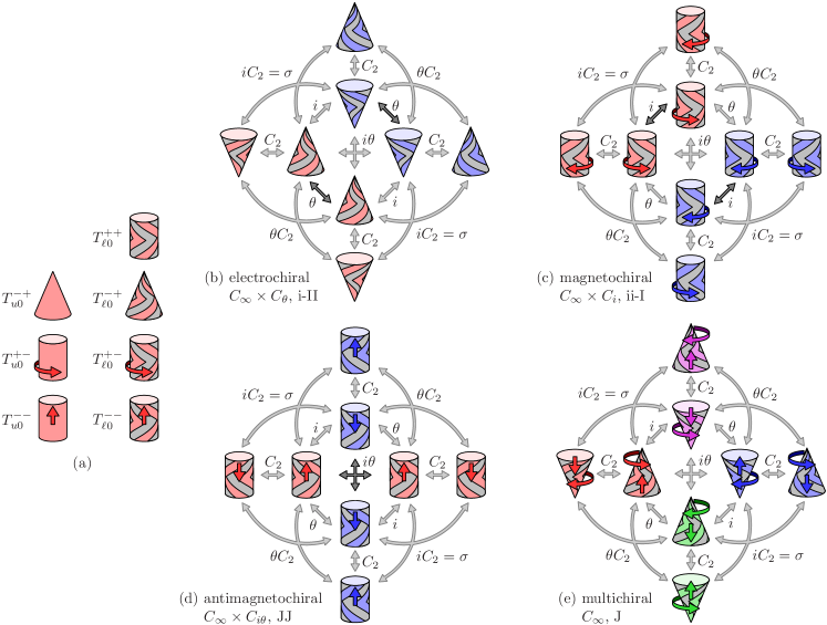
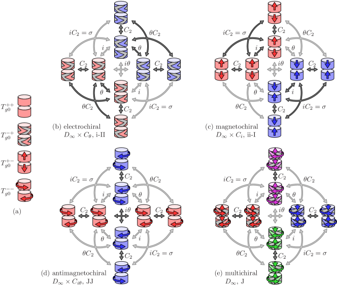
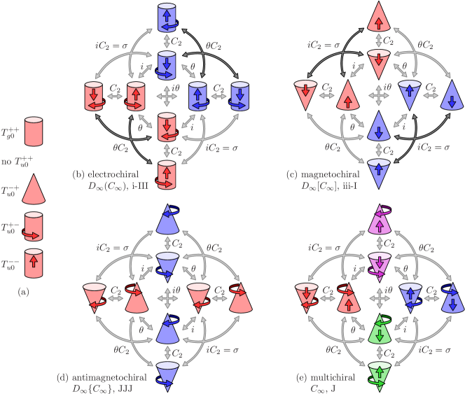
We now provide a brief overview of each category. Figures 2, 3 and 4 provide illustrative examples for these chiralities based on the continuous axial classes $L(C_{\infty})$ and $L(D_{\infty})$. These figures consider the symmetry transformations in the full axial rotation group $D_{\infty}\times C_{i\times\theta}$ to explore how different axially symmetric objects are either invariant (i.e., mapped onto themselves), mapped onto a rotated copy of themselves, or mapped onto distinct enantiomorphs. Materials candidates for the different categories of chirality are listed in Appendix F.

V.1.1 Parachirality

Parachiral point groups contain $\gamma$/̄improper rotations $\gamma C$ for all three inversions $\gamma=i$, $\theta$ and $i\theta$. Therefore, such systems have just one enantiomorph, i.e., the parachiral groups do not allow any kind of enantiomorphism. No scalars of $R_{i\times\theta}$ other than $T_{0}^{++}$ are permitted under parachiral groups. In particular, the scalar $T_{0}^{-+}$ is forbidden, and parachiral systems are therefore achiral as per the definition in Ref. [27]. Eight among the 15 group types defined in Table 2 are parachiral.

Examples of parachiral groups include the full axial rotation groups $C_{\infty}\times C_{i\times\theta}$ and $D_{\infty}\times C_{i\times\theta}$ permitting scalars $T_{\ell 0}^{++}$ and $T_{g0}^{++}$, respectively, as illustrated in Figs. 2(a), 3(a) and 4(a).

V.1.2 Electrochirality

Electrochiral groups contain $\theta$/̄improper rotations $\theta C$, but no $i$/̄improper or $i\theta$/̄improper rotations, i.e., an inequivalent enantiomorph is generated when a transformation $iC$ or $i\theta C$ is applied to the crystal. Electrochiral systems permit the pseudoscalar $T_{0}^{-+}$. See Figs. 2(b), 3(b), and 4(b) for illustrative examples.

Electrochiral groups are either electropolar (type LABEL:gcat:i-II) or multipolar (type LABEL:gcat:i-III). Electrochiral magnets belong to the latter type. Examples of nonmagnetic electrochiral systems are shown in Figs. 2(b) and 3(b). In these, chirality arises from the interplay of a parapolarization with an electropolarization, i.e., between even-$\ell$ and odd-$\ell$ electric-multipole densities. The scenario depicted in Fig. 4(b) is equivalent to an electrochiral ferromagnet, where electrochirality emerges from the presence of collinear magnetic and magnetotoroidal dipolarizations, which is the crystal analog of electrochirality arising when a magnetic field is applied parallel to a beam of light [83].

Electrochiral systems are optically active and they show a linear current-induced magnetization [89, 90, 91], though electrochirality is sufficient but not necessary for these effects [5, 27, 92].

V.1.3 Magnetochirality

Magnetochiral groups contain $i$/̄improper rotations $iC$, but $\theta$/̄improper and $i\theta$/̄improper rotations are absent. Therefore, any $\theta$/̄improper or $i\theta$/̄improper rotation generates an inequivalent enantiomorph of a system described by such a group. See Figs. 2(c), 3(c), and 4(c) for illustrative examples.

The nontrivial scalar allowed in magnetochiral groups is $T_{0}^{+-}$, which has no indicator associated with it in the electronic band structure, see Table 12 and Sec. V.2. Some physical consequences arising from the presence of $T_{0}^{+-}$ have recently been conjectured in Ref. [93]. As the scalar $T_{0}^{-+}$ is forbidden under magnetochiral groups, magnetochiral systems would be considered achiral according to Ref. [27]. However, the enantiomorphism arising under $\theta$/̄improper and $i\theta$/̄improper rotations makes magnetochiral systems fundamentally different from parachiral ones, as enantiomorphism is completely absent in the latter.

Magnetochiral groups are either magnetopolar (type LABEL:gcat:ii-I) or multipolar (type LABEL:gcat:iii-I). Examples of magnetopolar systems are shown in Figs. 2(c) and 3(c). Here enantiomorphism arises from the interplay of a parapolarization with a magnetopolarization, i.e., even/̄$\ell$ electric and odd/̄$\ell$ magnetic multipole densities. The scenario in Fig. 4(c) is an example of the multipolar type, which equivalently represents magnetochirality arising from collinear electric and magnetotoroidal dipolarizations. The same magnetochirality characterizes the situation where an electric field is applied parallel to a light beam.

V.1.4 Antimagnetochirality

Antimagnetochiral groups contain $i\theta$/̄improper rotations, but $i$/̄improper and $\theta$/̄improper rotations are absent. Thus, $\gamma$/̄improper rotations $\gamma C$, where $\gamma=i$ or $\theta$, generate an inequivalent enantiomorph of an antimagnetochiral structure. See the examples depicted in Figs. 2(d), 3(d), and 4(d).

The antimagnetochiral category subsumes what has previously been referred to as false chirality [83, 84]: although such a system exhibits enantiomorphism, it does not permit a scalar $T_{0}^{-+}$ and is therefore not considered to be truly chiral. Instead, a scalar $T_{0}^{--}$ is allowed in antimagnetochiral systems, though this scalar has no indicator associated with it in the electronic band structure, see Table 12 and Sec. V.2.

Antimagnetochiral groups are either antimagnetopolar (type LABEL:gcat:JJ) or multipolar (type LABEL:gcat:JJJ). Figures 2(d) and 3(d) show examples of antimagnetopolar antimagnetochiral systems, where antimagnetochirality arises from the combination of a parapolarization with an antimagnetopolarization. Figure 4(d) shows a multipolar system, representing also the situation where antimagnetochirality arises from the presence of collinear electric polarization and magnetization, or, equivalently, from parallel electric and magnetic fields [83].

V.1.5 Multichirality

Multichiral groups do not contain $\gamma$/̄improper rotations $\gamma C$ for any of the inversions $\gamma=i$, $\theta$ or $i\theta$. Hence, these groups coincide with the proper (type-LABEL:gcat:J) point groups. See Figs. 2(e), 3(e), and 4(e) for illustrative examples.

By the usual definition based on whether a scalar $T_{0}^{-+}$ is allowed [27], groups in the multichiral category have been classified as showing true chirality. However, they could equally be considered to exhibit false chirality [94]. Our more systematic analysis elucidates how the multichiral category differs fundamentally from both of these previously discussed chiralities. Firstly, this category has four distinct enantiomorphs, as all three improper rotations $iC$, $\theta C$ and $i\theta C$ yield distinct versions of the given object. See Figs. 2(e), 3(e), and 4(e). Secondly, all four scalars $T_{0}^{ss^{\prime}}$ are permitted under the multichiral groups, which thus combine the characteristics of electrochiral, magnetochiral and antimagnetochiral systems discussed above.

Multichiral systems are necessarily multipolar because coexisting chiralities require the interplay of a parapolarization with two different polarizations.

Table 15: Lowest-degree invariant tensors realizing chiralities in the continuous classes $L(R)$ and $L(D_{\infty})$, the cubic classes $L(O)$ and $L(T)$, and the axial classes $L(D_{n})$ and $L(C_{n})$ with $n=2,3,4,6$. We have $R\supset O\supset T$ and $D_{\infty}\supset D_{n}\supset C_{n}$, so that terms allowed under the respective supergroup are also allowed under the respective subgroup. cp denotes cyclic permutation of the preceding term and $(x\leftrightarrow y)$ denotes the preceding term with $x$ and $y$ interchanged. For the crystallographic classes, we denote in square brackets the degree $\ell$ of multipolar order represented by the respective terms as well as the maximal group that leaves this term invariant. For electrochirality and magnetochirality, we only consider electric and magnetic tensors with odd $\ell$; we do not consider toroidal compound tensors with even $\ell$. For antimagnetochirality, we consider the lowest-degree odd/̄$\ell$ magnetotoroidal compound tensors representing an antimagnetopolarization.
class $L(G_{\mathrm{p}})$ $L(R)$ $L(O)$ $L(T)$
$\rule{0.0pt}{11.62494pt}G_{\mathrm{p}}\times C_{i\times\theta}$ PC $k^{2}$ $[\ell=4,O\times C_{i\times\theta}]$ $k_{y}^{2}k_{z}^{2}+\mbox{cp}$
$[\ell=6,O\times C_{i\times\theta}]$ $\left[k_{x}^{4}(k_{y}^{2}+k_{z}^{2})+\mbox{cp}\right]-8k_{x}^{2}k_{y}^{2}k_{z}^{2}$ $[\ell=6,T\times C_{i\times\theta}]$ $(k_{y}^{2}-k_{z}^{2})(k_{z}^{2}-k_{x}^{2})(k_{x}^{2}-k_{y}^{2})$
$\rule{0.0pt}{11.62494pt}G_{\mathrm{p}}\times C_{\theta}$ EC ${\bm{\mathrm{\sigma}}}\cdot{\bm{\mathrm{k}}}$ $[\ell=9,O\times C_{\theta}]$
$\sigma_{x}k_{x}[k_{y}^{2}k_{z}^{2}(3k_{y}^{4}-10k_{y}^{2}k_{z}^{2}+3k_{z}^{4})$
$+k_{x}^{2}(k_{x}^{2}-k_{y}^{2}-k_{z}^{2})(k_{y}^{4}-6k_{y}^{2}k_{z}^{2}+k_{z}^{4})]+\mbox{cp}$
$[\ell=3,O[T]\times C_{\theta}]$ $\sigma_{x}k_{x}(k_{y}^{2}-k_{z}^{2})+\mbox{cp}$
$G_{\mathrm{p}}\times C_{i}$ MC $[\ell=9,O\times C_{i}]$ $\sigma_{x}k_{y}k_{z}(k_{y}^{2}-k_{z}^{2})[5k_{x}^{4}-3k_{x}^{2}(k_{y}^{2}+k_{z}^{2})+k_{y}^{2}k_{z}^{2}]+\mbox{cp}$ $[\ell=3,O(T)\times C_{i}]$ $\sigma_{x}k_{y}k_{z}+\mbox{cp}$
$G_{\mathrm{p}}\times C_{i\theta}$ AMC $[\ell=9,O\times C_{i\theta}]$ $k_{x}k_{y}k_{z}(k_{y}^{2}-k_{z}^{2})(k_{z}^{2}-k_{x}^{2})(k_{x}^{2}-k_{y}^{2})$ $[\ell=3,O(T)\times C_{i\theta}]$ $k_{x}k_{y}k_{z}$
class $L(G_{\mathrm{p}})$ $L(D_{\infty})$ $L(D_{6})$ $L(C_{6})$
$\rule{0.0pt}{11.62494pt}G_{\mathrm{p}}\times C_{i\times\theta}$ PC $k_{x}^{2}+k_{y}^{2};k_{z}^{2}$ $[\ell=6,D_{6}\times C_{i\times\theta}]$ $k_{x}^{2}(k_{x}^{2}-3k_{y}^{2})^{2};\;k_{y}^{2}(k_{y}^{2}-3k_{x}^{2})^{2}$ $[\ell=6,C_{6}\times C_{i\times\theta}]$ $k_{x}k_{y}(k_{x}^{2}-3k_{y}^{2})(k_{y}^{2}-3k_{x}^{2})$
$\rule{0.0pt}{11.62494pt}G_{\mathrm{p}}\times C_{\theta}$ EC
$\sigma_{x}k_{x}+\sigma_{y}k_{y};$
$\sigma_{z}k_{z}$
$[\ell=7,D_{12}[D_{6}]\times C_{\theta}]$
$\sigma_{x}k_{x}[k_{y}^{2}(k_{x}^{2}-3k_{y}^{2})(k_{y}^{2}-3k_{x}^{2})+3k_{z}^{2}(k_{x}^{4}-10k_{x}^{2}k_{y}^{2}+5k_{y}^{4})]$
$-(x\leftrightarrow y)-3\sigma_{z}k_{z}(k_{x}^{2}-k_{y}^{2})(k_{x}^{4}-14k_{x}^{2}k_{y}^{2}+k_{y}^{4})$
$[\ell=1,D_{\infty}[C_{\infty}]\times C_{\theta}]$ $\sigma_{x}k_{y}-\sigma_{y}k_{x}$
$G_{\mathrm{p}}\times C_{i}$ MC $[\ell=7,D_{12}(D_{6})\times C_{i}]$
$3\sigma_{x}k_{y}k_{z}(5k_{x}^{4}-10k_{x}^{2}k_{y}^{2}+k_{y}^{4})+(x\leftrightarrow y)$
$-\sigma_{z}k_{x}k_{y}(k_{x}^{2}-3k_{y}^{2})(k_{y}^{2}-3k_{x}^{2})$
$[\ell=1,D_{\infty}(C_{\infty})\times C_{i}]$ $\sigma_{z}$
$G_{\mathrm{p}}\times C_{i\theta}$ AMC $[\ell=7,D_{12}(D_{6})\times C_{i\theta}]$ $k_{x}k_{y}k_{z}(k_{x}^{2}-3k_{y}^{2})(k_{y}^{2}-3k_{x}^{2})$ $[\ell=1,D_{\infty}(C_{\infty})\times C_{i\theta}]$ $k_{z}$
class $L(G_{\mathrm{p}})$ $L(D_{3})$ $L(C_{3})$
$\rule{0.0pt}{11.62494pt}G_{\mathrm{p}}\times C_{i\times\theta}$ PC $[\ell=4,D_{3}\times C_{i\times\theta}]$ $k_{y}k_{z}(k_{y}^{2}-3k_{x}^{2})$ $[\ell=4,C_{3}\times C_{i\times\theta}]$ $k_{x}k_{z}(k_{x}^{2}-3k_{y}^{2})$
$\rule{0.0pt}{11.62494pt}G_{\mathrm{p}}\times C_{\theta}$ EC $[\ell=3,D_{6}[D_{3}]\times C_{\theta}]$ $2\sigma_{x}k_{z}k_{x}k_{y}+\sigma_{y}k_{z}(k_{x}^{2}-k_{y}^{2})+\sigma_{z}k_{y}(k_{y}^{2}-3k_{x}^{2})$ $[\ell=1,D_{\infty}[C_{\infty}]\times C_{\theta}]$ $\sigma_{x}k_{y}-\sigma_{y}k_{x}$
$G_{\mathrm{p}}\times C_{i}$ MC $[\ell=3,D_{6}(D_{3})\times C_{i}]$ $\sigma_{x}(k_{x}^{2}-k_{y}^{2})-2\sigma_{y}k_{x}k_{y}$ $[\ell=1,D_{\infty}(C_{\infty})\times C_{i}]$ $\sigma_{z}$
$G_{\mathrm{p}}\times C_{i\theta}$ AMC $[\ell=3,D_{6}(D_{3})\times C_{i\theta}]$ $k_{x}(k_{x}^{2}-3k_{y}^{2})$ $[\ell=1,D_{\infty}(C_{\infty})\times C_{i\theta}]$ $k_{z}$
class $L(G_{\mathrm{p}})$ $L(D_{4})$ $L(C_{4})$
$\rule{0.0pt}{11.62494pt}G_{\mathrm{p}}\times C_{i\times\theta}$ PC $[\ell=4,D_{4}\times C_{i\times\theta}]$ $k_{x}^{2}k_{y}^{2}$ $[\ell=4,C_{4}\times C_{i\times\theta}]$ $k_{x}k_{y}(k_{x}^{2}-k_{y}^{2})$
$\rule{0.0pt}{11.62494pt}G_{\mathrm{p}}\times C_{\theta}$ EC $[\ell=5,D_{8}[D_{4}]\times C_{\theta}]$
$\sigma_{x}k_{x}[k_{x}^{2}(k_{y}^{2}-k_{z}^{2})-k_{y}^{2}(k_{y}^{2}-3k_{z}^{2})]+(x\leftrightarrow y)$
$+\sigma_{z}k_{z}(k_{x}^{4}-6k_{x}^{2}k_{y}^{2}+k_{y}^{4})$
$[\ell=1,D_{\infty}[C_{\infty}]\times C_{\theta}]$ $\sigma_{x}k_{y}-\sigma_{y}k_{x}$
$G_{\mathrm{p}}\times C_{i}$ MC $[\ell=5,D_{8}(D_{4})\times C_{i}]$ $\sigma_{x}k_{y}k_{z}(k_{y}^{2}-3k_{x}^{2})-(x\leftrightarrow y)-\sigma_{z}k_{x}k_{y}(k_{x}^{2}-k_{y}^{2})$ $[\ell=1,D_{\infty}(C_{\infty})\times C_{i}]$ $\sigma_{z}$
$G_{\mathrm{p}}\times C_{i\theta}$ AMC $[\ell=5,D_{8}(D_{4})\times C_{i\theta}]$ $k_{x}k_{y}k_{z}(k_{x}^{2}-k_{y}^{2})$ $[\ell=1,D_{\infty}(C_{\infty})\times C_{i\theta}]$ $k_{z}$
class $L(G_{\mathrm{p}})$ $L(D_{2})$ $L(C_{2})$
$\rule{0.0pt}{11.62494pt}G_{\mathrm{p}}\times C_{i\times\theta}$ PC $[\ell=2,D_{2}\times C_{i\times\theta}]$ $k_{x}^{2}-k_{y}^{2};\;k_{y}^{2}-k_{z}^{2};\;k_{z}^{2}-k_{x}^{2}$ $[\ell=2,C_{2}\times C_{i\times\theta}]$ $k_{x}k_{y}$
$\rule{0.0pt}{11.62494pt}G_{\mathrm{p}}\times C_{\theta}$ EC $[\ell=3,O[T]\times C_{\theta}]$ $\sigma_{x}k_{x}(k_{y}^{2}-k_{z}^{2})+\mbox{cp}$ $[\ell=1,D_{\infty}[C_{\infty}]\times C_{\theta}]$ $\sigma_{x}k_{y}-\sigma_{y}k_{x}$
$G_{\mathrm{p}}\times C_{i}$ MC $[\ell=3,O(T)\times C_{i}]$ $\sigma_{x}k_{y}k_{z}+\mbox{cp}$ $[\ell=1,D_{\infty}(C_{\infty})\times C_{i}]$ $\sigma_{z}$
$G_{\mathrm{p}}\times C_{i\theta}$ AMC $[\ell=3,O(T)\times C_{i\theta}]$ $k_{x}k_{y}k_{z}$ $[\ell=1,D_{\infty}(C_{\infty})\times C_{i\theta}]$ $k_{z}$

V.2 Chirality and band structure

As discussed in Sec. IV and Ref. [22], the spin-dependent electronic band structure $E_{n\sigma}({\bm{\mathrm{k}}})$ directly reflects the categories of polarizations in solids. These categories manifest themselves via characteristic terms in the band structure that transform like irreducible tensors $T_{\ell}^{ss^{\prime}}$. In the following, we argue that the band structure $E_{n\sigma}({\bm{\mathrm{k}}})$ likewise reflects the categories of chirality in solids via an interplay of parapolar and unipolar (i.e., electropolar, magnetopolar, or antimagnetopolar) terms.

The categories of chirality can be defined via the criterion which monopoles $T_{0}^{ss^{\prime}}$ are permitted in a system, see Table 11. For example, in electrochiral crystal structures, the electrotoroidal compound scalar $T_{0}^{-+}$ becomes symmetry-allowed. In a band structure, such a scalar is realized by a term ${\bm{\mathrm{\sigma}}}\cdot{\bm{\mathrm{k}}}$. The presence of this scalar in a band structure has thus been identified as a key feature of electrochiral systems [88]. It can be viewed as a minimal model of an effective low-energy Hamiltonian for electrochirality in solids.

In contrast, using the same building blocks $k,\sigma$, the charges $T_{0}^{+-}$ and $T_{0}^{--}$ have no band-structure indicators associated with them (see Table 12). We can envision in magnetochiral systems (fictitious or engineered) compound scalars $T_{0}^{+-}\propto{\bm{\mathrm{d}}}\cdot{\bm{\mathrm{k}}}$ and in antimagnetochiral systems compound scalars $T_{0}^{--}\propto{\bm{\mathrm{\sigma}}}\cdot{\bm{\mathrm{d}}}$, where ${\bm{\mathrm{d}}}$ is an electric dipole density (signature $-+$) similar to the magnetic dipole density ${\bm{\mathrm{\sigma}}}$ (signature $+-$) [23].

However, for a crystal structure to be chiral, it is not decisive whether and how chiral charges $T_{0}^{ss^{\prime}}$ are actually realized. A monopole $T_{0}^{ss^{\prime}}$ is a sufficient, but not a necessary criterion for chirality in crystals. Electropolarizations, magnetopoloarizations, and antimagnetopolarizations $T_{\ell}^{ss^{\prime}}$ with $\ell>0$ combined with parapolarizations $T_{\ell}^{++}$ with $\ell>0$ can likewise make a system chiral. We show in the following how tensors $T_{\ell}^{ss^{\prime}}$ with $\ell>0$ can be used to define minimal models of effective low-energy Hamiltonians for electrochirality, magnetochirality and antimagnetochirality for all Laue classes $L(G_{\mathrm{p}})$.

Our theory is illustrated in Table 15 listing the lowest-degree invariant tensors realizing chiralities in the continuous classes $L(R)$ and $L(D_{\infty})$, the cubic classes $L(O)$ and $L(T)$, and the axial classes $L(D_{n})$ and $L(C_{n})$ with $n=2,3,4,6$.

Refer to caption
Figure 5: Chirality exhibited in the band structure for unipolar-unichiral groups in the classes $L(R)$ (left columns), $L(O)$ (center columns), and $L(T)$ (right columns). The first row shows energy surfaces of a parachiral system, whereas the second, third and fourth row show energy surfaces for the two enantiomorphs allowed under the indicated electrochiral, magnetochiral and antimagnetochiral groups.
Refer to caption
Figure 6: Unipolarizations giving rise to unichirality in the classes $L(T)$ (Fig. 5) and $L(C_{4})$ (Fig. 7) may also exist in systems with point groups in the classes $L(O)$ and $L(D_{4})$, respectively, where these terms, as shown here, do not give rise to unichirality.
Refer to caption
Figure 7: Chirality exhibited in the band structure for unipolar-unichiral groups in the classes $L(D_{\infty})$ (left columns), $L(D_{4})$ (center columns), and $L(C_{4})$ (right columns). The first row shows energy surfaces of a parachiral system, whereas the second, third and fourth row show energy surfaces for the two enantiomorphs allowed under the indicated electrochiral, magnetochiral and antimagnetochiral groups.

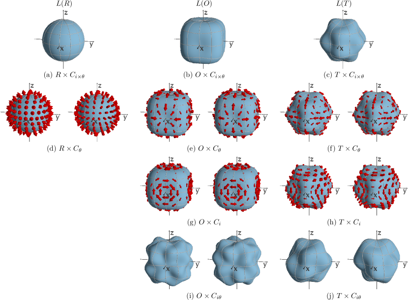
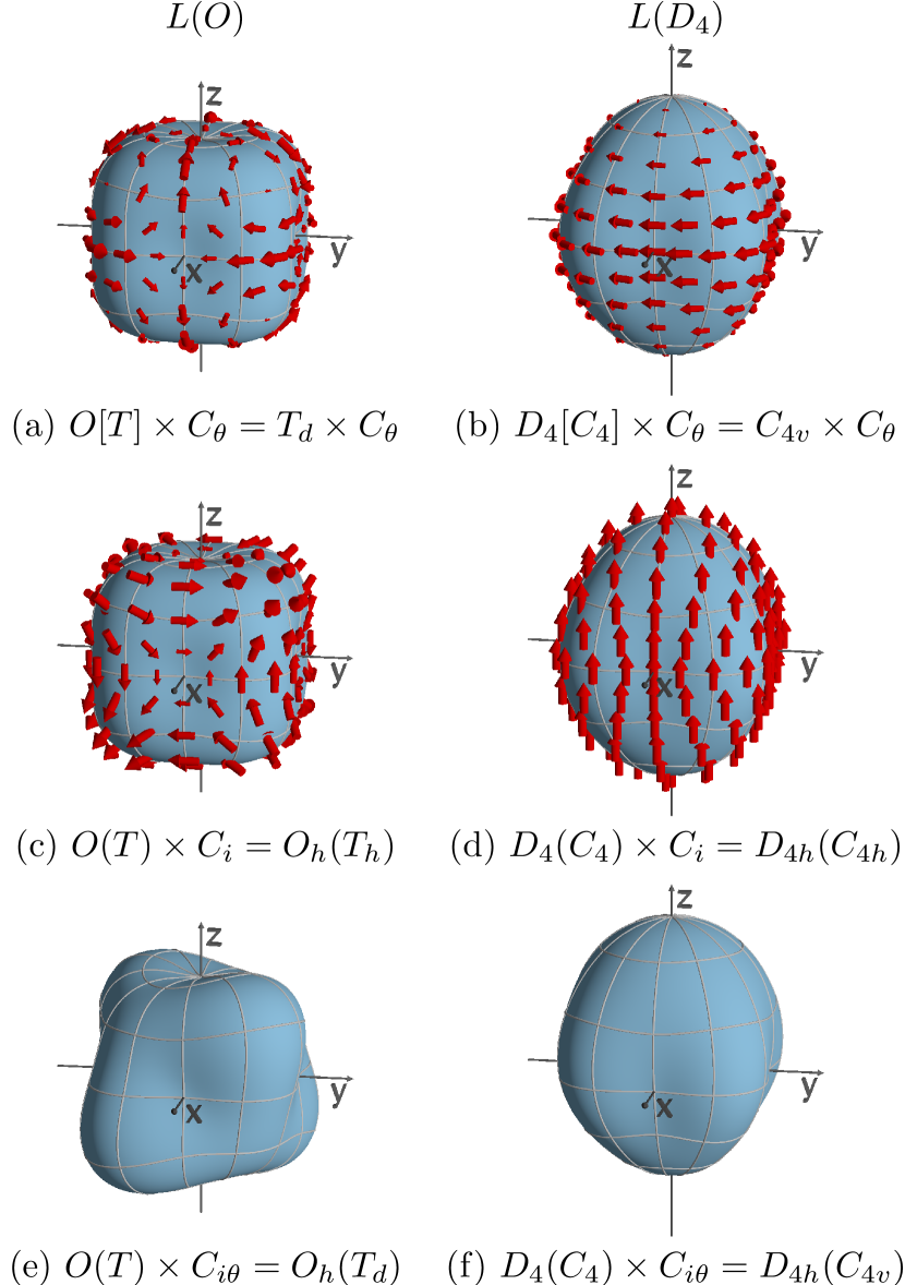
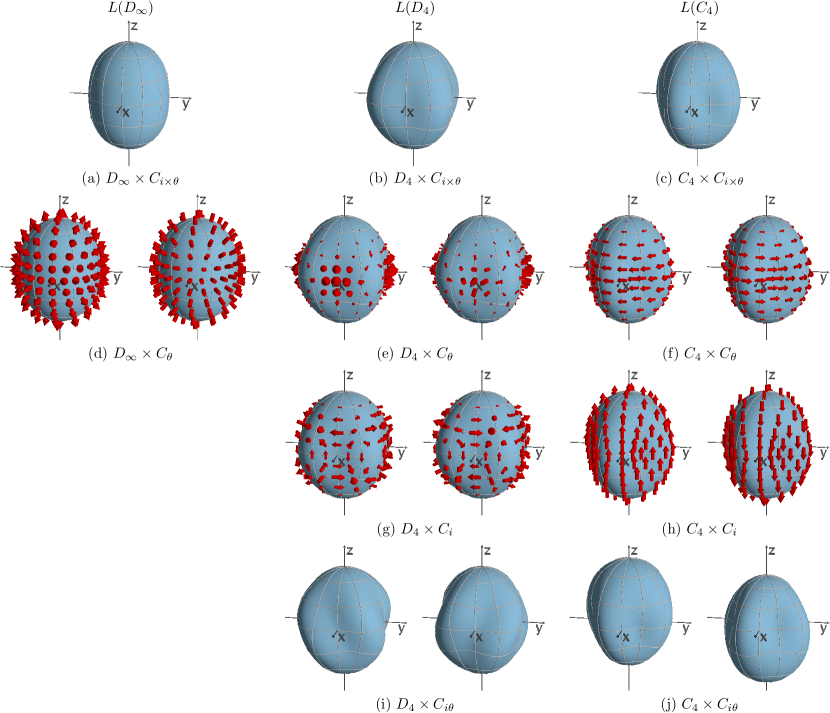
V.2.1 Spherical class $L(R)$

The full rotation group $R_{i\times\theta}$ is parachiral. The only invariant tensor permitted by this group is $T_{0}^{++}$ that is realized by the scalar $k^{2}$ and functions thereof [Fig 5(a)]. The electrochiral spherical group $R_{\theta}$ also permits a tensor $T_{0}^{-+}\propto{\bm{\mathrm{\sigma}}}\cdot{\bm{\mathrm{k}}}$ (and functions thereof). The latter term gives rise to two distinct enantiomorphs [95, 22, 96], see Fig 5(d). As discussed before, the magnetochiral group $R_{i}$ and the antimagnetochiral group $R_{i\theta}$ have no band structure indicators associated with them.

V.2.2 Cubic crystal system [classes $L(O)$ and $L(T)$]

Beyond the isotropic terms already permitted by the groups in the spherical class $L(R)$, all groups in the cubic class $L(O)$ also permit an electric hexadecapolarization ($\ell=4$) that manifests itself in lowest order via a term [22]

$$H^{(\mathrm{e},4)}\propto k_{x}^{2}k_{y}^{2}+k_{y}^{2}k_{z}^{2}+k_{z}^{2}k_{x}^{2}\,.$$ (22)

This term represents a warping of the energy dispersion $E_{\sigma}({\bm{\mathrm{k}}})$ of band electrons in cubic crystal structures [97, 98], see Fig 5(b).

The group $O\times C_{\theta}$ is electrochiral. In lowest order $\ell$, it permits an electropolarization with $\ell=9$ that gives rise to a term

$\displaystyle H^{(\mathrm{e},9)}\propto{}$ $\displaystyle\sigma_{x}k_{x}[k_{y}^{2}k_{z}^{2}(3k_{y}^{4}-10k_{y}^{2}k_{z}^{2}+3k_{z}^{4})$
$\displaystyle+k_{x}^{2}(k_{x}^{2}-k_{y}^{2}-k_{z}^{2})(k_{y}^{4}-6k_{y}^{2}k_{z}^{2}+k_{z}^{4})]+\mbox{cp}\,,$ (23)

see Fig. 5(e). The electrotoroidal scalar ${\bm{\mathrm{\sigma}}}\cdot{\bm{\mathrm{k}}}$ that is generally likewise present in such systems can be interpreted as a compound moment density (16) due to the combined effect of the electropolarization (23) and parapolarizations including the hexadecapolarization (22).

By SIS-TIS duality, the group $O\times C_{i}$ is magnetochiral. In lowest order $\ell$, it permits a magnetopolarization with $\ell=9$ that gives rise to a term

$\displaystyle H^{(\mathrm{m},9)}\propto{}$ $\displaystyle\sigma_{x}k_{y}k_{z}(k_{y}^{2}-k_{z}^{2})[5k_{x}^{4}-3k_{x}^{2}(k_{y}^{2}+k_{z}^{2})+k_{y}^{2}k_{z}^{2}]$
$\displaystyle\hskip 10.00002pt+\mbox{cp}\,,$ (24)

see Fig. 5(g). Finally, the group $O\times C_{i\theta}$ is antimagnetochiral. It permits an antimagnetopolarization ($\ell=0$) that manifests itself, in lowest order $\ell$, via a magnetotoroidal density with $\ell=9$ that gives rise to a term

$\displaystyle H^{(\mathrm{am},9)}\propto{}$ $\displaystyle k_{x}k_{y}k_{z}(k_{y}^{2}-k_{z}^{2})(k_{z}^{2}-k_{x}^{2})(k_{x}^{2}-k_{y}^{2})\,,$ (25)

see Fig. 5(i).

Besides the class $L(O)$, the cubic crystal system also includes the class $L(T)$. As $T\subset O$, the polarizations permitted by the point groups $G_{O}$ in $L(O)$ are also permitted by the respective groups $G_{T}\subset G_{O}$ in $L(T)$. Beyond that, the groups in $L(T)$ permit polarizations not present in $L(O)$, as listed in Table 15.

Specifically, the electrochiral group $T\times C_{\theta}$ permits an electric octupolarization $\ell=3$ that manifests itself via a Dresselhaus term

$$H^{(\mathrm{e},3)}\propto\sigma_{x}k_{x}(k_{y}^{2}-k_{z}^{2})+\mbox{cp}\,.$$ (26)

As is well known [77], this term is already allowed for systems with the parachiral point group $T_{d}\times C_{\theta}=O[T]\times C_{\theta}$ [Fig. 6(a)] realized, e.g., by the zincblende structure, i.e., by itself, this term is not sufficient as an indicator for electrochirality in the class $L(T)$. The Dresselhaus term (26) becomes an indicator for electrochirality [Fig. 5(f)] when combined with the parapolarization [$\ell=6$, Fig. 5(c)]

$$H^{(\mathrm{e},6)}\propto(k_{y}^{2}-k_{z}^{2})(k_{z}^{2}-k_{x}^{2})(k_{x}^{2}-k_{y}^{2})\,.$$ (27)

The parapolarization (27) is forbidden by the groups in the class $L(O)$, but it is allowed in the class $L(T)$. A parapolarization with $\ell=6$ that is allowed already in the class $L(O)$ is listed in Table 15.

Similarly, a magnetopolarization ($\ell=3$)

$$H^{(\mathrm{m},3)}\propto\sigma_{x}k_{y}k_{z}+\mbox{cp}$$ (28)

may exist in systems with magnetochiral group $T\times C_{i}$, but also in parachiral systems with point group $O(T)\times C_{i}$. The magnetopolarization (28) becomes an indicator for magnetochirality when combined with the parapolarization (27), see Fig. 5(h). Likewise, an antimagnetopolarization yields a magnetotoroidal density with $\ell=3$

$$H^{(\mathrm{am},3)}\propto k_{x}k_{y}k_{z}\,.$$ (29)

This density may exist in systems with antimagnetochiral group $T\times C_{i\theta}$, but also in parachiral systems with point group $O(T)\times C_{i\theta}$. The density (29) becomes an indicator for antimagnetochirality when combined with the parapolarization (27), see Fig. 5(j).

To summarize, in the class $L(T)$ the unipolar terms (26), (28), and (29) become indicators of electrochirality, magnetochirality, and antimagnetochirality, respectively, only when each of these terms is combined with the parapolarization (27), i.e., jointly the terms define minimal models for effective low-energy Hamiltonians realizing electrochirality (point group $T\times C_{\theta}$), magnetochirality ($T\times C_{i}$), and antimagnetochirality ($T\times C_{i\theta}$), respectively. This is discussed further in Sec. V.2.4.

V.2.3 Axial systems [classes $L(D_{n})$ and $L(C_{n})$]

Similar to the preceding discussion of the cubic classes $L(O)$ and $L(T)$, Table 15 also lists the lowest-order parapolar and unipolar tensors permitted by the class $L(D_{\infty})$, as well as the classes $L(D_{n})$ and $L(C_{n})$ with $n=2,3,4,6$. Figure 7 shows the chiral band structure for $L(D_{\infty})$, $L(D_{4})$, and $L(C_{4})$. For the dihedral classes $L(D_{6})$, $L(D_{3})$, $L(D_{4})$, and $L(D_{2})$ unichirality is realized by combining suitable parapolar terms with unipolar terms with $\ell=7$, 3, 5, and 3, respectively. Note that $D_{2}\subset T$ so that the class $L(D_{2})$ largely reproduces the features of the class $L(T)$.

The electropolar cyclic groups $C_{n}\times C_{\theta}$ permit a spontaneous electric dipolarization ($\ell=1$) that manifests itself via a Rashba term

$$H^{(\mathrm{e},1)}\propto\sigma_{x}k_{y}-\sigma_{y}k_{x}\,.$$ (30)

As is well known, this term is already allowed for systems with parachiral point groups $C_{nv}\times C_{\theta}=D_{n}[C_{n}]\times C_{\theta}$ realized, e.g., by the wurtzite structure ($C_{6v}\times C_{\theta}$) [76]. See also Fig. 6(b). When the Rashba term is combined with a suitable parapolar term forbidden by the class $L(D_{n})$, but allowed by the class $L(C_{n})$ (see Table 15), jointly these terms describe an electrochiral system [Fig. 7(f)].

Similarly, the cyclic groups $C_{n}\times C_{i}$ are magnetopolar, i.e., they permit a spontaneous magnetization ($\ell=1$) that manifests itself via an exchange (Zeeman) term

$$H^{(\mathrm{m},1)}\propto\sigma_{z}\,.$$ (31)

Such a term is already allowed for systems with the parachiral point groups $D_{n}(C_{n})\times C_{i}$, see Fig. 6(d). This term becomes an indicator of magnetochirality when combined with the respective parapolar terms listed for the classes $L(C_{n})$ in Table 15 [Fig. 7(h)].

Finally, the cyclic groups $C_{n}\times C_{i\theta}$ are antimagnetopolar, i.e., they permit a spontaneous antimagnetopolarization that manifests itself via a magnetotoroidal term ($\ell=1$)

$$H^{(\mathrm{am},1)}\propto k_{z}\,.$$ (32)

Again, such a term is already allowed for systems with the parachiral point groups $D_{n}(C_{n})\times C_{i\theta}$, see Fig. 6(f). This term becomes an indicator of antimagnetochirality when combined with the respective parapolar terms listed for the classes $L(C_{n})$ in Table 15 [Fig. 7(j)].

From a symmetry point of view, an electropolar system with spontaneous electric dipolarization (30) is equivalent to a parapolar system placed into an external electric field. In parapolar systems with crystallographic point group $C_{n}\times C_{i\times\theta}$, electrochirality can therefore be induced by placing the system into an external electric field [24]. Similarly, magnetochirality can be induced by placing such a system into an external magnetic field. Finally, parallel electric and magnetic fields make such systems multichiral, i.e., not only induce the fields a Rashba term (30) and a Zeeman term (31), but jointly the fields also induce a magnetotoroidal term (32).

V.2.4 Minimal effective models for chirality

Table 15 lists for each tabulated tensor its maximal group, i.e., the largest group that leaves the tensor invariant. For the odd/̄$\ell$ electropolar, magnetopolar and antimagnetopolar tensors, the respective maximal group is always an improper group beyond the class $L(G_{\mathrm{p}})$, so that these tensors, by themselves, cannot serve as minimal effective models for chirality in the class $L(G_{\mathrm{p}})$, as illustrated in Fig. 6.

Quite generally, a proper point group $G_{\mathrm{p}}$ is an invariant subgroup of $i$/̄minor groups $\tilde{G}_{\mathrm{p}}[G_{\mathrm{p}}]$

$$G_{\mathrm{p}}\subset\tilde{G}_{\mathrm{p}}[G_{\mathrm{p}}]\;,$$ (33a)
see Sec. II.2. Specifically, we have ($n=1,2,3,\ldots$)
$\displaystyle T$ $\displaystyle\subset T_{d}=O[T]$ (33b)
$\displaystyle D_{2n}$ $\displaystyle\subset D_{(2n)d}=D_{4n}[D_{2n}]$ (33c)
$\displaystyle D_{2n+1}$ $\displaystyle\subset D_{(2n+1)h}=D_{4n+2}[D_{2n+1}]$ (33d)
$\displaystyle C_{2n}$ $\displaystyle\subset\left\{\begin{array}[]{rl}S_{4n}&=C_{4n}[C_{2n}]\\ C_{(2n)v}&=D_{2n}[C_{2n}]\end{array}\right.$ (33g)
$\displaystyle C_{2n+1}$ $\displaystyle\subset\left\{\begin{array}[]{rl}C_{(2n+1)h}&=C_{4n+2}[C_{2n+1}]\\ C_{(2n+1)v}&=D_{2n+1}[C_{2n+1}]\end{array}\right.$ (33j)

and similar for the supergroups $\tilde{G}_{\mathrm{p}}(G_{\mathrm{p}})$ and $\tilde{G}_{\mathrm{p}}\{G_{\mathrm{p}}\}$ of $G_{\mathrm{p}}$. Of course, while a group like $D_{4}$ is a crystallographic point group, the supergroup $D_{4d}=D_{8}[D_{4}]\supset D_{4}$ is not a crystallographic point group. Nonetheless, the improper point group $D_{4d}$ is, ignoring TIS, the maximal group for the lowest-degree electropolar term permitted by the crystallographic point group $D_{4}$, see Table 15, so that this electropolar term, by itself, cannot serve as a minimal effective model for electrochirality in the class $L(D_{4})$.

Among the finite point groups, the octahedral group $O$ is special as it does not appear as a subgroup of a finite group outside the class $L(O)$. Therefore, the unipolar tensors with $\ell=9$ listed in Table 15 for the class $L(O)$ represent, by themselves, minimal effective models for unichirality in the class $L(O)$.

While the maximal groups for the unipolar tensors listed in Table 15 generally go beyond the respective class $L(G_{\mathrm{p}})$, for each of the parapolar tensors in Table 15 the maximal group is the full group $G_{\mathrm{p}}\times C_{i\times\theta}$ of the respective class. Therefore, jointly the unipolar tensors combined with the respective parapolar tensors represent minimal, effective models for unichirality in the class $L(G_{\mathrm{p}})$. Multichirality is realized by combining, at least, two different unipolar tensors in a class $L(G_{\mathrm{p}})$. Table 15 thus provides a complete theory for minimal effective models describing unipolar-unichiral and multipolar-multichiral systems [99].

The cooperation of a parapolarization and a unipolarization to realize unichirality can also be recognized in Fig. 2. In Fig. 2(a) we can envision that polar properties have been added to the parapolar nonchiral object $T_{\ell 0}^{++}$. Alternatively, we could imagine that the unipolar nonchiral objects $T_{u0}^{-+}$, $T_{u0}^{+-}$, and $T_{u0}^{--}$ have acquired a second nonpolar property so that jointly these properties realize chirality. These examples illustrate that we can generally have multiple pathways to realize chirality.

The multipolar-unichiral case in Fig. 4 is different from the unipolar-unichiral case in Figs. 2 and 3. The objects shown in Fig. 4(a) visualize the irreducible tensors $T_{g0}^{++}$ and $T_{u0}^{-+}$, $T_{u0}^{+-}$, and $T_{u0}^{--}$ as indicated. While individual objects $T_{u0}^{ss^{\prime}}$ in Fig. 4(a) are unipolar but not chiral, it is the superposition of their polarizations that yields unichirality [Figs. 4(b) to (d)] and multichirality [Fig. 4(e)].

This rule applies also to minimal effective models for chirality in multipolar-unichiral systems. For example, the multipolar-electrochiral group $D_{4}(C_{4})$ permits the electropolar term

$\displaystyle H^{(\mathrm{e},5)}\propto{}$ $\displaystyle\sigma_{x}k_{x}[k_{x}^{2}(k_{y}^{2}-k_{z}^{2})-k_{y}^{2}(k_{y}^{2}-3k_{z}^{2})]+(x\leftrightarrow y)$
$\displaystyle+\sigma_{z}k_{z}(k_{x}^{4}-6k_{x}^{2}k_{y}^{2}+k_{y}^{4})\,,$ (34)

[because $D_{4}(C_{4})\subset D_{4}\times C_{\theta}\subset D_{8}[D_{4}]\times C_{\theta}$, see Table 15 and Fig. 1], the magnetopolar term (31) [because $D_{4}(C_{4})\subset D_{4}(C_{4})\times C_{i}$, see Table 15], and the antimagnetopolar term (32) [because $D_{4}(C_{4})\subset D_{4}(C_{4})\times C_{i\theta}$]. Any two of these terms are sufficient as a minimal model for electrochirality under $D_{4}(C_{4})$ because the largest subgroup common to any two of the three groups $D_{4}\times C_{\theta}$, $D_{4}(C_{4})\times C_{i}$, and $D_{4}(C_{4})\times C_{i\theta}$ is $D_{4}(C_{4})$. Of course, $D_{4}(C_{4})$ permits not only the electropolar term (34), but also the parapolar term

$$H^{(\mathrm{e},4)}\propto k_{x}^{2}k_{y}^{2}$$ (35)

because $D_{4}(C_{4})\subset D_{4}\times C_{i\times\theta}$, see Table 15. Jointly, the terms (34) and (35) can serve not only as a minimal model for electrochirality under $D_{4}\times C_{\theta}$, but also under $D_{4}(C_{4})\subset D_{4}\times C_{\theta}$.

Using Table 15, minimal models for other multipolar-unichiral systems can be constructed in a similar way. We thus have a complete theory for minimal effective models describing chirality in crystals [99]. Our analysis shows that chirality in solid-state systems is qualitatively different from chirality in molecules and elementary-particle physics.

VI Conclusions and outlook

Using symmetry as a fundamental guiding principle, we have developed a comprehensive theory of electromagnetism and chirality in crystalline solids. We have identified five categories of electric and magnetic multipole order and five categories of chirality that provide a complementary, comprehensive classification of crystal structures and their physical properties. The categories yield 15 types of crystal structures with distinctive electric and magnetic properties. Multiple versions of chirality that were previously overlooked, including multichirality with four distinct enantiomorphs are a novel criterion underlying our comprehensive classification. Our work shows explicitly how chirality is linked to electromagnetic order and band structure.

Clearly, the concept of SIS-TIS duality, Eq. (7), can be extended from abstract group theory to a duality of physical quantities and effects characterizing crystal structures. For example, an electric field ${\bm{\mathcal{E}}}$ and a magnetic field ${\bm{\mathcal{B}}}$ can be considered duals of each other in the sense that the groups according to which fields ${\bm{\mathcal{E}}}$ and ${\bm{\mathcal{B}}}$ transform are related by $i\leftrightarrow\theta$ duality; see Table 10. This implies, in turn, that physical effects associated with fields ${\bm{\mathcal{E}}}$ and ${\bm{\mathcal{B}}}$ can likewise be related by $i\leftrightarrow\theta$ duality. A simple example is the electric response of a medium to an electric field. The dual effect is the magnetic response of a medium to a magnetic field. The magnetoelectric effect can be considered a self-dual effect. From a different perspective, pairs of material tensors can be related by $i\leftrightarrow\theta$ duality if they are permitted under dual pairs of magnetic groups, see Tables 2, 3, 5, 8 and 9 and Appendix E. Examples of pairs of dual tensors are given by the rank/̄1 pyroelectric and pyromagnetic tensors and the rank/̄3 piezoelectric and piezomagnetic tensors, while the rank/̄2 magnetoelectric tensor is self-dual [100].

A more thorough analysis of duality-related physical effects also needs to consider Onsager’s reciprocal relations accounting for the symmetry of fluctuations under time inversion $\theta$ when studying irreversible processes [101]. In the context of magnetic systems breaking TIS such an analysis is not trivial. For example, following early work [102], the symmetry of the conductivity tensor describing the anomalous Hall effect in magnetically ordered systems was discussed intensely till a consensus was reached. See Ref. [103]. A proper discussion of this important point is beyond the scope of the present work. It will be the subject of a future publication.

Acknowledgements.
RW and UZ acknowledge stimulating discussions with N. Spaldin. RW also benefited from discussions with R. Cavanaugh, A. Hoffmann, L. Lurio, and M. Norman. UZ thanks S. Marsland for useful comments on an early version of the manuscript. Work at Argonne was supported by DOE BES under Contract No. DE-AC02-06CH11357.

Appendix A Refined symmetry classifications

This Appendix contains a general discussion of the group-theoretical framework underlying the refined symmetry classifications used in this work. Appendix A.2 comments briefly on spin groups.

A.1 General formalism

Starting from the 11 crystallographic point groups $G_{\mathrm{p}}$ of proper rotations, symmetry classifications of crystal structures can be systematically refined by permitting a wider range of symmetry elements in the symmetry groups for these systems. Formally, the construction of nonmagnetic point groups, magnetic point groups, and even spin point groups by combining groups $G_{\mathrm{p}}$ of proper rotations with space inversion $i$ [6], time inversion $\theta$ [14] and spin rotations [104] follows a similar scheme, where each set of additional symmetries permits a more fine-grained classification of the symmetry groups $H$ that can be realized by physical systems compared with the symmetry groups $G$ that arise in a coarse-grained symmetry analysis [105]. The additional symmetries are generally characterized by a symmetry group $\bar{G}$, and we want to explore the possibilities how the symmetries in $\bar{G}$ can be combined with the symmetries in $G$ to form new symmetry groups $H$.

Two limiting cases are trivial. First, the symmetry group remains $G$ if all symmetries in $\bar{G}$ are broken. Second, the symmetry group becomes the product group $\bar{G}\times G$ if all symmetries in $\bar{G}$ are by themselves good symmetries of the system. Nontrivial scenarios arise if symmetries represented by elements in $\bar{G}$ are by themselves broken, but these elements must be combined with symmetry elements in $G$ to obtain new good symmetries of the system. To identify and describe these scenarios in a systematic way [6, 14, 104], we consider all subgroups $\bar{U}_{1}$ and $\bar{U}_{2}$ of $\bar{G}$ with $\bar{U}_{1}\cap\bar{U}_{2}=\{e\}$. We assume that the group $\bar{U}_{1}$ contains the symmetry elements in $\bar{G}$ that are good symmetries of a system independent of the symmetries in $G$, whereas $\bar{U}_{2}$ contains the symmetry elements in $\bar{G}$ that must be combined with elements in $G$ to form a group $\bar{H}(\bar{U}_{2},G)$. The symmetry groups $H$ then become

$$H=\bar{U}_{1}\times\bar{H}(\bar{U}_{2},G)\,.$$ (36)

We obtain the admissible groups $\bar{H}(\bar{U}_{2},G)$ via the homomorphism theorem for groups [106]. Given $G$ and $\bar{U}_{2}$, we identify all invariant subgroups $U$ of $G$ such that $\bar{U}_{2}$ is isomorphic to the factor group $G/U$. Then we obtain $\bar{H}(\bar{U}_{2},G)$ by combining the cosets for the invariant subgroup $U$ of $G$ with the elements in $\bar{U}_{2}$, consistent with the isomorphism relating $\bar{U}_{2}$ and $G/U$. By definition, $\bar{H}$ is isomorphic to $G$. The order of the group $H$ equals the order of $G$ times the order of $\bar{U}_{1}$.

If we combine the 11 groups $G=G_{\mathrm{p}}$ of proper rotations with the space inversion group $\bar{G}=C_{i}$, the symmetry groups $H$ are the 32 nonmagnetic crystallographic point groups. More specifically, the two-element group $\bar{G}=C_{i}$ permits three cases. (i) When $\bar{U}_{1}=\bar{U}_{2}=\{e\}$, Eq. (36) yields the type/̄i groups $G_{\mathrm{p}}$. (ii) When $\bar{U}_{1}=C_{i}$ and $\bar{U}_{2}=\{e\}$, we get the type/̄ii groups $C_{i}\times G_{\mathrm{p}}$. (iii) Finally, $\bar{U}_{1}=\{e\}$ and $\bar{U}_{2}=C_{i}$ yields the type/̄iii groups, consistent with the discussion in Sec. II.2 and Eq. (5b).

In the same way, combining the 32 nonmagnetic crystallographic point groups with the time inversion group $\bar{G}=C_{\theta}$ yields the 122 magnetic point groups (types I, II, and III) that are further classified in Tables 2 and 9.

A.2 Spin groups

Equation (36) can also be used to derive spin groups [104, 107, 108] that recently have received renewed interest [38, 39]. While the following discussion can readily be generalized to space groups, for clarity we focus on point groups only. Generally, the symmetry elements $g$ in nonmagnetic crystallographic point groups can be associated with operators $\hat{g}$ that represent transformations $C_{g}$ of the position vector ${\bm{\mathrm{r}}}$

$${\bm{\mathrm{r}}}^{\prime}=\hat{g}\,{\bm{\mathrm{r}}}=C_{g}\,{\bm{\mathrm{r}}}\,.$$ (37)

These operators $\hat{g}$ also describe the transformation of scalar property functions of a crystal structure such as the charge density $\rho({\bm{\mathrm{r}}})$

$$\hat{g}\,\rho({\bm{\mathrm{r}}}^{\prime})=\rho({\bm{\mathrm{r}}})\qquad\mathrm{or}\qquad\hat{g}\,\rho({\bm{\mathrm{r}}})=\rho(C_{g}^{-1}{\bm{\mathrm{r}}})\,.$$ (38)

Then we associate a nonmagnetic symmetry group $G$ with a crystallographic structure if for all $g\in G$ the operators $\hat{g}$ leave the scalar function $\rho({\bm{\mathrm{r}}})$ invariant

$$\hat{g}\,\rho({\bm{\mathrm{r}}})=\rho(C_{g}^{-1}{\bm{\mathrm{r}}})=\rho({\bm{\mathrm{r}}})\,.$$ (39)

Magnetic crystal structures have a magnetization density ${\bm{\mathcal{m}}}({\bm{\mathrm{r}}})$ that is characterized not only by a nontrivial behavior under the black-white symmetry time inversion $\theta$. But similar to Eq. (38) we have

$$\hat{h}\,{\bm{\mathcal{m}}}({\bm{\mathrm{r}}})=\bar{C}_{h}\,{\bm{\mathcal{m}}}(C_{h}^{-1}{\bm{\mathrm{r}}})\,,$$ (40)

that is, the symmetry group becomes an extended group $H$ as in Eq. (36), where we associate with each $h\in H$ a transformation $C_{h}$ of the position vector ${\bm{\mathrm{r}}}$ and a transformation $\bar{C}_{h}$ of the vector ${\bm{\mathcal{m}}}$. We have $C_{h}=\mathcal{C}\mathcal{I}$ where $\mathcal{C}\in R$ is a proper rotation and $\mathcal{I}\in C_{i}$, whereas $\bar{C}_{h}=\bar{\mathcal{C}}\mathcal{T}$ with $\bar{\mathcal{C}}\in R$ and $\mathcal{T}\in C_{\theta}$. This is consistent with the signature $-+$ ($+-$) of ${\bm{\mathrm{r}}}$ (${\bm{\mathcal{m}}}$). The invariance condition for ${\bm{\mathcal{m}}}({\bm{\mathrm{r}}})$ then becomes

$$\hat{h}\,{\bm{\mathcal{m}}}({\bm{\mathrm{r}}})=\bar{C}_{h}\,{\bm{\mathcal{m}}}(C_{h}^{-1}{\bm{\mathrm{r}}})={\bm{\mathcal{m}}}({\bm{\mathrm{r}}})\,.$$ (41)

Magnetic groups combine nonmagnetic groups $G$ with $\bar{G}=C_{\theta}$ so that the transformations $\bar{C}_{h}$ and $C_{h}$ in Eq. (41) have the same proper rotational parts, $\bar{\mathcal{C}}=\mathcal{C}$. Spin groups, on the other hand, combine nonmagnetic groups $G$ (that are subgroups of $R_{i}\equiv R\times C_{i}$) with groups $\bar{U}_{1},\bar{U}_{2}\subset\bar{G}=R_{\theta}\equiv R\times C_{\theta}$ to obtain a more fine-grained classification of the symmetries of a magnetization density ${\bm{\mathcal{m}}}({\bm{\mathrm{r}}})$. Here, the decomposition $\bar{U}_{1}\times\bar{U}_{2}\subset R_{\theta}$ with $\bar{U}_{1}\cap\bar{U}_{2}=\{e\}$ yields five cases [104]. (i) The trivial case $\bar{U}_{1}=\bar{U}_{2}=\{e\}$ yields spin groups that are equivalent to the magnetic type/̄I groups. (ii) Similarly, $\bar{U}_{1}=R_{\theta}$ and $\bar{U}_{2}=\{e\}$ is equivalent to the magnetic type II. (iii) $\bar{U}_{1}=D_{\infty}(C_{\infty})$ (which is the dual of $D_{\infty}[C_{\infty}]=C_{\infty v}$) implies $\bar{U}_{2}=C_{\theta}$. Here the groups $\bar{H}(C_{\theta},G)$ are the type/̄III magnetic groups. This case represents collinear magnetization densities ${\bm{\mathcal{m}}}({\bm{\mathrm{r}}})$. (iv) $\bar{U}_{1}=C_{2}(C_{1})$ (which is the dual of $C_{2}[C_{1}]=C_{s}$) implies that $\bar{U}_{2}$ is a subgroup of $D_{\infty}(C_{\infty})$, i.e., $\bar{U}_{2}$ is the dual of one of the nonmagnetic crystallographic groups $G\subset D_{\infty}[C_{\infty}]=C_{\infty v}$. This case represents planar magnetization densities ${\bm{\mathcal{m}}}({\bm{\mathrm{r}}})$. (v) Finally, we may have $\bar{U}_{1}=\{e\}$ and $\bar{U}_{2}\neq\{e\}$, i.e., $\bar{U}_{2}$ is the dual of one of the 32 nonmagnetic crystallographic groups. This case represents spatial magnetization densities ${\bm{\mathcal{m}}}({\bm{\mathrm{r}}})$. For the group $G=O_{h}$, the spin point groups are tabulated in Ref. [104]. Reference [108] tabulates all spin point groups for cases (iii), (iv) and (v), though without referencing the cases they apply to. More recently, spin groups have also been tabulated in Ref. [109].

Clearly, spin groups can be further generalized using $\bar{G}=R_{i\times\theta}$ [110] which is appropriate for magnetic structures with not only a magnetization density ${\bm{\mathcal{m}}}({\bm{\mathrm{r}}})$ ($\ell=1$ and signature $+-$) but also, e.g., a magnetic quadrupole density ($\ell=2$ and signature $--$) [17, 22]. The general case $\bar{G}=R_{i\times\theta}$ also represents electropolar and multipolar structures with electric multipole densities.

Appendix B Form of subclasses $\boldsymbol{L(G_{0}^{i\theta},i\theta)}$

The concept of subclasses of magnetic point groups is introduced in Sec. II.5. While the form of subclasses $L(G_{0}^{i},i)$ and $L(G_{0}^{\theta},\theta)$ is straightforward, the form of subclasses $L(G_{0}^{i\theta},i\theta)$ discussed in the following is more subtle.

Every magnetic point group $G\in L(G_{\mathrm{p}})$ has the general form [31]

$$G=\tilde{G}_{\mathrm{p}}+i\{g_{\nu}^{(i)}\}+\theta\{g_{\nu}^{(\theta)}\}+i\theta\{g_{\nu}^{(i\theta)}\}\,\,.$$ (42)

Here $\tilde{G}_{\mathrm{p}}\subseteq G_{\mathrm{p}}$ is a proper point group, and $\{g_{\nu}^{(\gamma)}\}$ denotes the set of operations in the class root $G_{\mathrm{p}}$ that appears in $G$ in combination with the black-white symmetry element $\gamma\in\{i,\theta,i\theta\}$. In the following, we assume $G\supsetneq G_{\mathrm{p}}$, i.e., at least one set $\{g_{\nu}^{(\gamma)}\}$ is nonempty. The relation $\gamma^{2}=e$ and general group properties of $G$ imply the relations

$\displaystyle g_{\nu}^{(\gamma)}g_{\mu}^{(\gamma)}$ $\displaystyle\in\tilde{G}_{\mathrm{p}}$ $\displaystyle\mbox{for any fixed $\gamma$}\,\,,$ (43a)
$\displaystyle g_{\nu}^{(\gamma)}g_{\mu}^{(\gamma^{\prime})}$ $\displaystyle\in\{g_{\nu^{\prime}}^{(\gamma\gamma^{\prime})}\}$ $\displaystyle\mbox{for any pair $\gamma\neq\gamma^{\prime}$}\,\,.$ (43b)

It follows from Eq. (43b) that either only one set $\{g_{\nu}^{(\gamma)}\}$ is nonempty, or all three sets are nonempty.

To understand how the mapping $i\theta\mapsto e$ transforms the group $G$ given in Eq. (42), we first note

$$\theta=i^{2}\,\theta=i\,i\theta\;\stackrel{{\scriptstyle i\theta\mapsto e}}{{\longmapsto}}\;i$$ (44a)
to find
$$G\;\stackrel{{\scriptstyle i\theta\mapsto e}}{{\longmapsto}}\;G^{i\theta}_{0}\equiv\tilde{G}_{\mathrm{p}}+\{g_{\nu}^{(i\theta)}\}+i\big{(}\{g_{\nu}^{(i)}\}+\{g_{\nu}^{(\theta)}\}\big{)}\,,$$ (44b)

where clearly $G^{i\theta}_{0}$ is again a group. Alternatively, using

$$i=i\,\theta^{2}=i\theta\,\theta\;\stackrel{{\scriptstyle i\theta\mapsto e}}{{\longmapsto}}\;\theta$$ (45a)
yields
$$G\;\stackrel{{\scriptstyle i\theta\mapsto e}}{{\longmapsto}}\;G_{0\mathrm{d}}^{i\theta}\equiv\tilde{G}_{\mathrm{p}}+\{g_{\nu}^{(i\theta)}\}+\theta\big{(}\{g_{\nu}^{(i)}\}+\{g_{\nu}^{(\theta)}\}\big{)}\,\,.$$ (45b)

Thus we can identify two equivalent subclass roots $G_{0}^{i\theta}\leftrightarrow G_{0\mathrm{d}}^{i\theta}$ that are related via the duality transformation $i\leftrightarrow\theta$, and

$$L(G_{0}^{i\theta},i\theta)\equiv L(G_{0\mathrm{d}}^{i\theta},i\theta)\;.$$ (46)

Applying the duality transformation $i\leftrightarrow\theta$ to $G$ in Eq. (42) yields the dual partner

$$G\;\leftrightarrow\;G_{\mathrm{d}}=\tilde{G}_{\mathrm{p}}+\theta\{g_{\nu}^{(i)}\}+i\{g_{\nu}^{(\theta)}\}+i\theta\{g_{\nu}^{(i\theta)}\}\,\,.$$ (47)

Equations (44a) and (45a) show that $G_{\mathrm{d}}$ maps to the same subclass roots $G^{i\theta}_{0}\leftrightarrow G_{0\mathrm{d}}^{i\theta}$ as $G$, i.e., dual partners $G$ and $G_{\mathrm{d}}$ belong to the same subclass $L(G_{0}^{i\theta},i\theta)\equiv L(G_{0\mathrm{d}}^{i\theta},i\theta)$.

Specializing the composition of a subclass $L(G_{0}^{\gamma},\gamma)$ discussed generally in Sec. II.5 to the case $\gamma=i\theta$, we find that $L(G_{\mathrm{p}},i\theta)$ contains besides $G_{\mathrm{p}}$ also GLABEL:gcat:JJ=Gp×Ciθsubscript𝐺LABEL:gcat:JJsubscript𝐺psubscript𝐶𝑖𝜃G_{\mathrm{\ref{gcat:JJ}}}=G_{\mathrm{p}}\times C_{i\theta} and all the type/̄LABEL:gcat:JJJ groups $G_{\mathrm{p}}\{\tilde{G}_{\mathrm{p}}\}\in L(G_{\mathrm{p}})$. It follows from Eqs. (44a) and (45a) that the subclass $L(G_{\mathrm{p}}\times C_{i},i\theta)\equiv L(G_{\mathrm{p}}\times C_{\theta},i\theta)$ contains the groups of type LABEL:gcat:ii-II, LABEL:gcat:ii-I and LABEL:gcat:i-II as well as all type-LABEL:gcat:ii-III and type-LABEL:gcat:iii-II groups in $L(G_{\mathrm{p}})$. Groups in a subclass $L(G_{\mathrm{p}}[\tilde{G}_{\mathrm{p}}],i\theta)\equiv L(G_{\mathrm{p}}(\tilde{G}_{\mathrm{p}}),i\theta)$ contain, besides $G_{\mathrm{p}}[\tilde{G}_{\mathrm{p}}]$ and $G_{\mathrm{p}}(\tilde{G}_{\mathrm{p}})$, also the type/̄LABEL:gcat:JJp group $G_{\mathrm{p}}(\tilde{G}_{\mathrm{p}})\times C_{i\theta}$. Furthermore, GLABEL:gcat:JJJp=Gp[G~p(1)](G~p(1)[Gp])subscript𝐺LABEL:gcat:JJJpsubscript𝐺pdelimited-[]superscriptsubscript~𝐺p1superscriptsubscript~𝐺psuperscript1delimited-[]subscript𝐺pG_{\mathrm{\ref{gcat:JJJp}}}=G_{\mathrm{p}}[\tilde{G}_{\mathrm{p}}^{(1)}]\,(\tilde{G}_{\mathrm{p}}^{(1^{\prime})}[\accentset{\approx}{G}_{\mathrm{p}}]) is in $L(G_{\mathrm{p}}[\tilde{G}_{\mathrm{p}}^{(2)}],i\theta)\equiv L(G_{\mathrm{p}}(\tilde{G}_{\mathrm{p}}^{(2)}),i\theta)$, while GLABEL:gcat:iii-IIIp=Gp[G~p(1)](G~p(2)[Gp])subscript𝐺LABEL:gcat:iii-IIIpsubscript𝐺pdelimited-[]superscriptsubscript~𝐺p1superscriptsubscript~𝐺p2delimited-[]subscript𝐺pG_{\mathrm{\ref{gcat:iii-IIIp}}}=G_{\mathrm{p}}[\tilde{G}_{\mathrm{p}}^{(1)}]\,(\tilde{G}_{\mathrm{p}}^{(2)}[\accentset{\approx}{G}_{\mathrm{p}}]) and GLABEL:gcat:iiip-III=Gp(G~p(1))[G~p(2)(Gp)]subscript𝐺LABEL:gcat:iiip-IIIsubscript𝐺psuperscriptsubscript~𝐺p1delimited-[]superscriptsubscript~𝐺p2subscript𝐺pG_{\mathrm{\ref{gcat:iiip-III}}}=G_{\mathrm{p}}(\tilde{G}_{\mathrm{p}}^{(1)})\,[\tilde{G}_{\mathrm{p}}^{(2)}(\accentset{\approx}{G}_{\mathrm{p}})] both belong to $L(G_{\mathrm{p}}[\tilde{G}_{\mathrm{p}}^{(1)}],i\theta)\equiv L(G_{\mathrm{p}}(\tilde{G}_{\mathrm{p}}^{(1)}),i\theta)$.

The combination of $L(G_{\mathrm{p}},i\theta)$ with $L(G_{\mathrm{p}}\times C_{i},i\theta)\equiv L(G_{\mathrm{p}}\times C_{\theta},i\theta)$ and all subclasses $L(G_{\mathrm{p}}[\tilde{G}_{\mathrm{p}}],i\theta)\equiv L(G_{\mathrm{p}}(\tilde{G}_{\mathrm{p}}),i\theta)$ yields the class $L(G_{\mathrm{p}})$ [Eq. (12)].

Appendix C IRs of the continuous axial groups

This Appendix reviews the IRs of the continuous axial groups that we refer to repeatedly in this work. The cyclic groups $G_{c\infty}$ are Abelian so that all their IRs are one-dimensional. Under these groups, the transformation behavior of tensor components $T_{\ell m}^{ss^{\prime}}$ of $R_{i\times\theta}$ depends only on $m$ but not on $\ell$; for fixed $m$ but different values of $\ell$ (with $|m|\leq\ell$), the components $T_{\ell m}^{ss^{\prime}}$ transform the same way under groups $G_{c\infty}$. The invariant tensors of groups $G_{c\infty}$ are then the tensor components $T_{\ell 0}^{ss^{\prime}}$ (Table 6). Similar to $T_{00}^{++}$ under the spherical groups, tensor components $T_{\ell 0}^{++}$ are invariant under all cyclic groups $G_{c\infty}$.

The dihedral groups $G_{d\infty}$ are nonabelian. Under groups $G_{d\infty}$, the tensor components $T_{\ell 0}^{ss^{\prime}}$ of $R_{i\times\theta}$ transform according to one-dimensional IRs, whereas tensor components $T_{\ell,\pm m}^{ss^{\prime}}$ with $m\neq 0$ pairwise transform according to two-dimensional IRs. More specifically, the transformation properties depend on the parity of $\ell$. For even $\ell$ (“$g$”), tensor components $T_{g0}^{ss^{\prime}}$ are even under $\pi$ rotations $C_{2}$ about an axis perpendicular to the main axis of the dihedral groups (chosen as the $z$ axis in Table 7), whereas for odd $\ell$ (“$u$”), tensor components $T_{u0}^{ss^{\prime}}$ are odd under rotations $C_{2}$. The invariant tensor components $T_{\ell 0}^{ss^{\prime}}$ under the dihedral groups $G_{d\infty}$ thus distinguish between $\ell$ even or odd, see Table 7. But similar to tensor components $T_{\ell 0}^{ss^{\prime}}$ under the cyclic groups, tensor components with different even or different odd values of $\ell$ behave the same.

According to the general definition of group types given in Table 2, the continuous dihedral groups have the group types listed in the first column of Table 7. A comparison of Tables 7 and 11 shows that the range of multipole densities $T_{\ell}^{ss^{\prime}}$ permitted by these continuous dihedral groups falls short of the range of densities generally permitted by the categories of polarization associated with these group types. For example, the group $D_{\infty}\times C_{\theta}$ has the type LABEL:gcat:i-II that belongs to the electropolar category. But the group $D_{\infty}\times C_{\theta}$ does not allow odd/̄$\ell$ electric multipoles ($-+$). This result can be traced back to the fact that the groups in the class $L(D_{\infty})$ can also be viewed as limiting groups $n\rightarrow\infty$ for the groups in the class $L(D_{n})$. The lowest degree $\ell_{\min}^{(e,u)}$ of odd/̄$\ell$ electric multipoles permitted by groups $D_{n}\times C_{\theta}$ grows monotonically with increasing $n$, with $\ell_{\min}^{(e,u)}\rightarrow\infty$ for $n\rightarrow\infty$ (see Table 18). This does not affect our classification of categories of polarized matter as crystals are characterized by finite crystallographic point groups.

Table 16 gives the multiplication table for the eight one-dimensional IRs of $D_{\infty}\times C_{i\times\theta}$ with $m=0$. Our notation for these IRs used in Table 16 indicates that we may use as $1\times 1$ representation matrices the $m=0$ diagonal elements $d_{\ell}^{ss^{\prime}}\equiv(D_{\ell}^{ss^{\prime}})_{00}$ of the representation matrices $D_{\ell}^{ss^{\prime}}$ of $R_{i\times\theta}$ with $\ell$ even (“g”) and $\ell$ odd (“u”). More specifically, Table 16 reflects the fact that the Clebsch-Gordan coefficients $(\ell_{1}0,\ell_{2}0|\ell_{1}\ell_{2},\ell 0)$ in Eq. (16) are nonzero only if $\ell_{1}+\ell_{2}+\ell$ is even [56]. Note that dg++𝟙superscriptsubscript𝑑𝑔absent𝟙d_{g}^{++}\equiv\openone becomes the identity representation of $D_{\infty}\times C_{i\times\theta}$.

The dihedral groups $D_{\infty}\langle C_{\infty}\rangle_{\gamma}$ leave tensor components $T_{\ell 0}^{ss^{\prime}}$ with even and odd $\ell$ invariant. Note that it follows from the multiplication table 16 that, in these groups, the chiral charges $T_{g0}^{ss^{\prime}}$ arise as compound tensors that are products of the respective invariant tensor components $T_{u0}^{ss^{\prime}}$.

Table 16: Multiplication table for the IRs with $m=0$ of the full axial rotation group $D_{\infty}\times C_{i\times\theta}$. Our notation for these IRs indicates that we may use as $1\times 1$ representation matrices the $m=0$ diagonal elements $d_{\ell}^{ss^{\prime}}\equiv(D_{\ell}^{ss^{\prime}})_{00}$ of the representation matrices $D_{\ell}^{ss^{\prime}}$ of $R_{i\times\theta}$ with $\ell$ even (“$g$”) and $\ell$ odd (“$u$”). Note that dg++𝟙superscriptsubscript𝑑𝑔absent𝟙d_{g}^{++}\equiv\openone becomes the identity representation of $D_{\infty}\times C_{i\times\theta}$.
$\rule{0.0pt}{11.62494pt}d_{g}^{++}$ $d_{g}^{-+}$ $d_{g}^{+-}$ $d_{g}^{--}$ $d_{u}^{++}$ $d_{u}^{-+}$ $d_{u}^{+-}$ $d_{u}^{--}$
$\rule{0.0pt}{11.62494pt}d_{g}^{++}$ $d_{g}^{-+}$ $d_{g}^{+-}$ $d_{g}^{--}$ $d_{u}^{++}$ $d_{u}^{-+}$ $d_{u}^{+-}$ $d_{u}^{--}$ $d_{g}^{++}$
$d_{g}^{++}$ $d_{g}^{--}$ $d_{g}^{+-}$ $d_{u}^{-+}$ $d_{u}^{++}$ $d_{u}^{--}$ $d_{u}^{+-}$ $d_{g}^{-+}$
$d_{g}^{++}$ $d_{g}^{-+}$ $d_{u}^{+-}$ $d_{u}^{--}$ $d_{u}^{++}$ $d_{u}^{-+}$ $d_{g}^{+-}$
$d_{g}^{++}$ $d_{u}^{--}$ $d_{u}^{+-}$ $d_{u}^{-+}$ $d_{u}^{++}$ $d_{g}^{--}$
$d_{g}^{++}$ $d_{g}^{-+}$ $d_{g}^{+-}$ $d_{g}^{--}$ $d_{u}^{++}$
$d_{g}^{++}$ $d_{g}^{--}$ $d_{g}^{+-}$ $d_{u}^{-+}$
$d_{g}^{++}$ $d_{g}^{-+}$ $d_{u}^{+-}$
$d_{g}^{++}$ $d_{u}^{--}$

The cyclic groups in Table 6 are subgroups of the dihedral groups in Table 7. The maximal groups of tensor components $T_{\ell 0}^{ss^{\prime}}$ are thus generally the dihedral groups that provide a more fine-grained classification of the symmetries of $T_{\ell 0}^{ss^{\prime}}$ based on the parity of $\ell$, see Table 7.

Interestingly, inspection of Table 7 shows that a tensor component $T_{u0}^{++}$ is not invariant under any of the continuous dihedral groups. It is only invariant under continuous cyclic groups $G_{c\infty}$, including $C_{\infty}\times C_{i\times\theta}$, that do not distinguish between tensor components $T_{u0}^{++}$ and $T_{g0}^{++}$. We note that all tensor components $T_{\ell m}^{ss^{\prime}}$ are unambiguously defined via the IRs of the spherical group $R_{i\times\theta}$, even though discussing these tensor components in conjunction with smaller groups like $C_{i\times\theta}$ [31, 68] and cyclic or dihedral groups [47] can be instructive.

Axial quantities were previously discussed, e.g., in Refs. [47] and [50]. To ease cross-referencing between these works and ours, we provide Table 17 relating respective notations for axial quantities. The multiplication table 16 is consistent with Table 1 of Ref. [50], but it is at variance with Table V of Ref. [47].

Table 17: Notation for axial quantities in the literature. Ref. [47] uses the symbols from Ref. [68] for tensor components $T_{u0}^{ss^{\prime}}$.
This work $T_{g0}^{++}$ $T_{g0}^{-+}$ $T_{g0}^{+-}$ $T_{g0}^{--}$ $T_{u0}^{++}$ $T_{u0}^{-+}$ $T_{u0}^{+-}$ $T_{u0}^{--}$
Ref. [47] ${\bm{\mathrm{N}}}$ ${\bm{\mathrm{C}}}$ ${\bm{\mathrm{L}}}$ ${\bm{\mathrm{F}}}$ ${\bm{\mathrm{G}}}$ ${\bm{\mathrm{P}}}$ ${\bm{\mathrm{M}}}$ ${\bm{\mathrm{T}}}$
Ref. [50] $\mathcal{D}$ $\mathcal{C}$ $\mathcal{D}^{\prime}$ $\mathcal{C}^{\prime}$

$\displaystyle\mathcal{a}$

$\mathcal{P}$ $\scalebox{1.2}{\mbox{$\displaystyle\mathcal{a}$}}^{\prime}$ $\mathcal{P}^{\prime}$

Appendix D Spherical tensors and multipole order permitted by the 122 crystallographic magnetic point groups

This Appendix provides explicit details about which spherical tensors $T_{\ell}^{ss^{\prime}}$ are permitted by the 122 crystallographic magnetic point groups. The information given here is directly relevant for discussing electric, magnetic and toroidal multipole order in crystals, see Sec. IV.2. As discussed below, the information is furthermore relevant for materials and property tensors that are commonly represented by Cartesian rank/̄$N$ tensors.

Table 18: Number of independent components of $\theta$/̄even spherical tensors $T_{\ell}^{s+}$ permitted by type/̄II magnetic point groups (considering ranks $\ell\leq 3$). Tensors $T_{\ell}^{++}$ represent parapolarizations and $T_{\ell}^{-+}$ are electropolarizations. A “0” indicates that the tensor is forbidden by symmetry. The electric monopolarization $T_{0}^{++}$ has been omitted, as it is trivially always allowed. The quantities $\ell_{\mathrm{min}}^{(\mathrm{e/et,g/u})}$ indicate, respectively, for each group, the lowest symmetry-allowed even (“$g$”) and odd (“$u$”) orders $\ell$ of electric (“e”) and electrotoroidal (“et”) multipole densities, again ignoring the electric monopolarization, except for the spherical groups for which it is the only allowed parapolarization. Both the Schönflies and Hermann-Mauguin notations [111] are given for each group, as well as the group’s type according to the classification in Table 2.
parapolar electropolar
Crystal system Schönflies Hermann- Mauguin type $\ell_{\min}^{(e,g)}$ $\ell_{\min}^{(et,u)}$ $T_{1}^{++}$ $T_{2}^{++}$ $T_{3}^{++}$ $\ell_{\min}^{(et,g)}$ $\ell_{\min}^{(e,u)}$ $T_{0}^{-+}$ $T_{1}^{-+}$ $T_{2}^{-+}$ $T_{3}^{-+}$
Triclinic $C_{1}\times C_{\theta}$ $=C_{1}\times C_{\theta}$ $1^{\prime}$ i-II $2$ $1$ $3$ $5$ $7$ 00 $1$ $1$ $3$ $5$ $7$
$C_{1}\times C_{i\times\theta}$ $=C_{i}\times C_{\theta}$ $\bar{1}1^{\prime}$ ii-II $2$ $1$ $3$ $5$ $7$ $\infty$ $\infty$ 00 00 00 00
Monoclinic $C_{2}\times C_{\theta}$ $=C_{2}\times C_{\theta}$ $21^{\prime}$ i-II $2$ $1$ $1$ $3$ $3$ 00 $1$ $1$ $1$ $3$ $3$
$C_{2}[C_{1}]\times C_{\theta}$ $=C_{s}\times C_{\theta}$ $m1^{\prime}$ iii-II $2$ $1$ $1$ $3$ $3$ $2$ $1$ 00 $2$ $2$ $4$
$C_{2}\times C_{i\times\theta}$ $=C_{2h}\times C_{\theta}$ $2/m1^{\prime}$ ii-II $2$ $1$ $1$ $3$ $3$ $\infty$ $\infty$ 00 00 00 00
Orthorhombic $D_{2}\times C_{\theta}$ $=D_{2}\times C_{\theta}$ $2221^{\prime}$ i-II $2$ $3$ 00 $2$ $1$ 00 $3$ $1$ 00 $2$ $1$
$D_{2}[C_{2}]\times C_{\theta}$ $=C_{2v}\times C_{\theta}$ $mm21^{\prime}$ iii-II $2$ $3$ 00 $2$ $1$ $2$ $1$ 00 $1$ $1$ $2$
$D_{2}\times C_{i\times\theta}$ $=D_{2h}\times C_{\theta}$ $mmm1^{\prime}$ ii-II $2$ $3$ 00 $2$ $1$ $\infty$ $\infty$ 00 00 00 00
Tetragonal $C_{4}\times C_{\theta}$ $=C_{4}\times C_{\theta}$ $41^{\prime}$ i-II $2$ $1$ $1$ $1$ $1$ 00 $1$ $1$ $1$ $1$ $1$
$C_{4}[C_{2}]\times C_{\theta}$ $=S_{4}\times C_{\theta}$ $\bar{4}1^{\prime}$ iii-II $2$ $1$ $1$ $1$ $1$ $2$ $3$ 00 00 $2$ $2$
$C_{4}\times C_{i\times\theta}$ $=C_{4h}\times C_{\theta}$ $4/m1^{\prime}$ ii-II $2$ $1$ $1$ $1$ $1$ $\infty$ $\infty$ 00 00 00 00
$D_{4}\times C_{\theta}$ $=D_{4}\times C_{\theta}$ $4221^{\prime}$ i-II $2$ $5$ 00 $1$ 00 00 $5$ $1$ 00 $1$ 00
$D_{4}[C_{4}]\times C_{\theta}$ $=C_{4v}\times C_{\theta}$ $4mm1^{\prime}$ iii-II $2$ $5$ 00 $1$ 00 $4$ $1$ 00 $1$ 00 $1$
$D_{4}[D_{2}]\times C_{\theta}$ $=D_{2d}\times C_{\theta}$ $\bar{4}2m1^{\prime}$ iii-II $2$ $5$ 00 $1$ 00 $2$ $3$ 00 00 $1$ $1$
$D_{4}\times C_{i\times\theta}$ $=D_{4h}\times C_{\theta}$ $4/mmm1^{\prime}$ ii-II $2$ $5$ 00 $1$ 00 $\infty$ $\infty$ 00 00 00 00
Trigonal $C_{3}\times C_{\theta}$ $=C_{3}\times C_{\theta}$ $31^{\prime}$ i-II $2$ $1$ $1$ $1$ $3$ 00 $1$ $1$ $1$ $1$ $3$
$C_{3}\times C_{i\times\theta}$ $=C_{3i}\times C_{\theta}$ $\bar{3}1^{\prime}$ ii-II $2$ $1$ $1$ $1$ $3$ $\infty$ $\infty$ 00 00 00 00
$D_{3}\times C_{\theta}$ $=D_{3}\times C_{\theta}$ $321^{\prime}$ i-II $2$ $3$ 00 $1$ $1$ 00 $3$ $1$ 00 $1$ $1$
$D_{3}[C_{3}]\times C_{\theta}$ $=C_{3v}\times C_{\theta}$ $3m1^{\prime}$ iii-II $2$ $3$ 00 $1$ $1$ $4$ $1$ 00 $1$ 00 $2$
$D_{3}\times C_{i\times\theta}$ $=D_{3d}\times C_{\theta}$ $\bar{3}m1^{\prime}$ ii-II $2$ $3$ 00 $1$ $1$ $\infty$ $\infty$ 00 00 00 00
Hexagonal $C_{6}\times C_{\theta}$ $=C_{6}\times C_{\theta}$ $61^{\prime}$ i-II $2$ $1$ $1$ $1$ $1$ 00 $1$ $1$ $1$ $1$ $1$
$C_{6}[C_{3}]\times C_{\theta}$ $=C_{3h}\times C_{\theta}$ $\bar{6}1^{\prime}$ iii-II $2$ $1$ $1$ $1$ $1$ $4$ $3$ 00 00 00 $2$
$C_{6}\times C_{i\times\theta}$ $=C_{6h}\times C_{\theta}$ $6/m1^{\prime}$ ii-II $2$ $1$ $1$ $1$ $1$ $\infty$ $\infty$ 00 00 00 00
$D_{6}\times C_{\theta}$ $=D_{6}\times C_{\theta}$ $6221^{\prime}$ i-II $2$ $7$ 00 $1$ 00 00 $7$ $1$ 00 $1$ 00
$D_{6}[C_{6}]\times C_{\theta}$ $=C_{6v}\times C_{\theta}$ $6mm1^{\prime}$ iii-II $2$ $7$ 00 $1$ 00 $6$ $1$ 00 $1$ 00 $1$
$D_{6}[D_{3}]\times C_{\theta}$ $=D_{3h}\times C_{\theta}$ $\bar{6}m21^{\prime}$ iii-II $2$ $7$ 00 $1$ 00 $4$ $3$ 00 00 00 $1$
$D_{6}\times C_{i\times\theta}$ $=D_{6h}\times C_{\theta}$ $6/mmm1^{\prime}$ ii-II $2$ $7$ 00 $1$ 00 $\infty$ $\infty$ 00 00 00 00
Cubic $T\times C_{\theta}$ $=T\times C_{\theta}$ $231^{\prime}$ i-II $4$ $3$ 00 00 $1$ 00 $3$ $1$ 00 00 $1$
$T\times C_{i\times\theta}$ $=T_{h}\times C_{\theta}$ $m31^{\prime}$ ii-II $4$ $3$ 00 00 $1$ $\infty$ $\infty$ 00 00 00 00
$O\times C_{\theta}$ $=O\times C_{\theta}$ $4321^{\prime}$ i-II $4$ $9$ 00 00 00 00 $9$ $1$ 00 00 00
$O[T]\times C_{\theta}$ $=T_{d}\times C_{\theta}$ $\bar{4}3m1^{\prime}$ iii-II $4$ $9$ 00 00 00 $6$ $3$ 00 00 00 $1$
$O\times C_{i\times\theta}$ $=O_{h}\times C_{\theta}$ $m3m1^{\prime}$ ii-II $4$ $9$ 00 00 00 $\infty$ $\infty$ 00 00 00 00
Number of crystallographic groups allowing tensor $13$ $27$ $21$ $11$ $10$ $13$ $18$
Axial $C_{\infty}\times C_{\theta}$ $=C_{\infty}\times C_{\theta}$ $\infty 1^{\prime}$ i-II $2$ $1$ $1$ $1$ $1$ 00 $1$ $1$ $1$ $1$ $1$
$C_{\infty}\times C_{i\times\theta}$ $=C_{\infty h}\times C_{\theta}$ $\infty/m1^{\prime}$ ii-II $2$ $1$ $1$ $1$ $1$ $\infty$ $\infty$ 00 00 00 00
$D_{\infty}\times C_{\theta}$ $=D_{\infty}\times C_{\theta}$ $\infty 21^{\prime}$ i-II $2$ $\infty$ 00 $1$ 00 00 $\infty$ $1$ 00 $1$ 00
$D_{\infty}[C_{\infty}]\times C_{\theta}$ $=C_{\infty v}\times C_{\theta}$ $\infty m1^{\prime}$ iii-II $2$ $\infty$ 00 $1$ 00 $\infty$ $1$ 00 $1$ 00 $1$
$D_{\infty}\times C_{i\times\theta}$ $=D_{\infty h}\times C_{\theta}$ $\infty/mm1^{\prime}$ ii-II $2$ $\infty$ 00 $1$ 00 $\infty$ $\infty$ 00 00 00 00
Spherical $R\times C_{\theta}$ $=R_{\theta}$ $\infty\infty 1^{\prime}$ i-II 00 $\infty$ 00 00 00 00 $\infty$ $1$ 00 00 00
$R\times C_{i\times\theta}$ $=R_{i\times\theta}$ $\infty\infty m1^{\prime}$ ii-II 00 $\infty$ 00 00 00 $\infty$ $\infty$ 00 00 00 00

Table 18 is devoted to $\theta$/̄even tensors $T_{\ell}^{s+}$. It lists the number of independent components such tensors with rank $\ell\leq 3$ have under the nonmagnetic (type/̄II) groups belonging to the 11 Laue classes $L(G_{\mathrm{p}})$. For comparison, the same information is also provided for type/̄II groups in the three classes of continuous cyclic, dihedral and spherical point groups. To streamline the presentation, the universally allowed electric monopolarization $T_{0}^{++}$ has been omitted. Basic physical properties can be read off from this table. For example, groups allowing $T_{0}^{-+}$ represent electrochiral systems, see Sec. V.1.2, and groups allowing $T_{1}^{-+}$ represent pyroelectric and ferroelectric systems [5].

Table 18 together with Table 9 can be used to infer the properties of tensors $T_{\ell}^{s+}$ in all 122 magnetic point groups. Specifically, Table 18 gives the properties of tensors for the crystallographic point groups $G_{0}^{\theta}\times C_{\theta}$ that appear in Table 9 in the last row of the main block [52] for a class $L(G_{\mathrm{p}})$. The structure of tensors $T_{\ell}^{s+}$ allowed under $G_{0}^{\theta}\times C_{\theta}$ is repeated for all members of the subclass $L(G_{0}^{\theta},\theta)\subset L(G_{\mathrm{p}})$, which are the groups positioned in the column headed by $G_{0}^{\theta}$ within the same class’s main block. The formal basis for these congruences is elaborated in detail in Appendix E.

Table 18 also tabulates the lowest even (“$g$”) and odd (“$u$”) orders $\ell$ of electric (“e”) and electrotoroidal (“et”) multipole densities permitted in each crystal class. The electric monopolarization $T_{0}^{++}$ is trivially allowed under all point groups and, therefore, is not considered for determining $\ell_{\mathrm{min}}^{(\mathrm{e,g})}$ (except for spherical groups where it is the only allowed parapolarization). Instead, to convey information that is specific to each group, we tabulate the lowest nonzero even order of parapolarizations allowed under each group.

Table 19: Number of independent components of $\theta$/̄odd spherical tensors $T_{\ell}^{s-}$ permitted by type/̄III magnetic point groups (considering ranks $\ell\leq 3$). Tensors $T_{\ell}^{+-}$ represent magnetopolarizations and $T_{\ell}^{--}$ are antimagnetopolarizations. A “0” indicates that the corresponding tensor is forbidden by symmetry. The magnetic monopolarization $T_{0}^{+-}$ has been omitted, as it is universally forbidden under type/̄III groups. The quantities $\ell_{\mathrm{min}}^{(\mathrm{m/mt,g/u})}$ indicate, respectively, for each group, the lowest symmetry-allowed even (“$g$”) and odd (“$u$”) orders $\ell$ of magnetic (“m”) and magnetotoroidal (“mt”) multipole densities. Both the Schönflies and Hermann-Mauguin notations [111] are given for each group, as well as the group’s type according to the classification in Table 2.
magnetopolar antimagnetopolar
Crystal system Schönflies Hermann- Mauguin type $\ell_{\min}^{(mt,g)}$ $\ell_{\min}^{(m,u)}$ $T_{1}^{+-}$ $T_{2}^{+-}$ $T_{3}^{+-}$ $\ell_{\min}^{(m,g)}$ $\ell_{\min}^{(mt,u)}$ $T_{0}^{--}$ $T_{1}^{--}$ $T_{2}^{--}$ $T_{3}^{--}$
Triclinic $C_{1}\times C_{i\theta}$ $=C_{i}(C_{1})$ $\bar{1}^{\prime}$ JJ $\infty$ $\infty$ 00 00 00 00 $1$ $1$ $3$ $5$ $7$
Monoclinic $C_{2}(C_{1})$ $=C_{2}(C_{1})$ $2^{\prime}$ i-III $2$ $1$ $2$ $2$ $4$ $2$ $1$ 00 $2$ $2$ $4$
$C_{2}\{C_{1}\}$ $=C_{s}(C_{1})$ $m^{\prime}$ JJJ $2$ $1$ $2$ $2$ $4$ 00 $1$ $1$ $1$ $3$ $3$
$C_{2}(C_{1})\times C_{i}$ $=C_{2h}(C_{i})$ $2^{\prime}/m^{\prime}$ ii-III $2$ $1$ $2$ $2$ $4$ $\infty$ $\infty$ 00 00 00 00
$C_{2}\times C_{i\theta}$ $=C_{2h}(C_{2})$ $2/m^{\prime}$ JJ $\infty$ $\infty$ 00 00 00 00 $1$ $1$ $1$ $3$ $3$
$C_{2}(C_{1})\times C_{i\theta}$ $=C_{2h}(C_{s})$ $2^{\prime}/m$ JJ’ $\infty$ $\infty$ 00 00 00 $2$ $1$ 00 $2$ $2$ $4$
Orthorhombic $D_{2}(C_{2})$ $=D_{2}(C_{2})$ $2^{\prime}2^{\prime}2$ i-III $2$ $1$ $1$ $1$ $2$ $2$ $1$ 00 $1$ $1$ $2$
$D_{2}\{C_{2}\}$ $=C_{2v}(C_{2})$ $m^{\prime}m^{\prime}2$ JJJ $2$ $1$ $1$ $1$ $2$ 00 $3$ $1$ 00 $2$ $1$
$D_{2}[C_{2}](C_{2}[C_{1}])$ $=C_{2v}(C_{s})$ $2^{\prime}m^{\prime}m$ JJJ” $2$ $1$ $1$ $1$ $2$ $2$ $1$ 00 $1$ $1$ $2$
$D_{2}(C_{2})\times C_{i}$ $=D_{2h}(C_{2h})$ $mm^{\prime}m^{\prime}$ ii-III $2$ $1$ $1$ $1$ $2$ $\infty$ $\infty$ 00 00 00 00
$D_{2}\times C_{i\theta}$ $=D_{2h}(D_{2})$ $m^{\prime}m^{\prime}m^{\prime}$ JJ $\infty$ $\infty$ 00 00 00 00 $3$ $1$ 00 $2$ $1$
$D_{2}(C_{2})\times C_{i\theta}$ $=D_{2h}(C_{2v})$ $mmm^{\prime}$ JJ’ $\infty$ $\infty$ 00 00 00 $2$ $1$ 00 $1$ $1$ $2$
Tetragonal $C_{4}(C_{2})$ $=C_{4}(C_{2})$ $4^{\prime}$ i-III $2$ $3$ 00 $2$ $2$ $2$ $3$ 00 00 $2$ $2$
$C_{4}\{C_{2}\}$ $=S_{4}(C_{2})$ $\bar{4}^{\prime}$ JJJ $2$ $3$ 00 $2$ $2$ 00 $1$ $1$ $1$ $1$ $1$
$C_{4}(C_{2})\times C_{i}$ $=C_{4h}(C_{2h})$ $4^{\prime}/m$ ii-III $2$ $3$ 00 $2$ $2$ $\infty$ $\infty$ 00 00 00 00
$C_{4}\times C_{i\theta}$ $=C_{4h}(C_{4})$ $4/m^{\prime}$ JJ $\infty$ $\infty$ 00 00 00 00 $1$ $1$ $1$ $1$ $1$
$C_{4}(C_{2})\times C_{i\theta}$ $=C_{4h}(S_{4})$ $4^{\prime}/m^{\prime}$ JJ’ $\infty$ $\infty$ 00 00 00 $2$ $3$ 00 00 $2$ $2$
$D_{4}(D_{2})$ $=D_{4}(D_{2})$ $4^{\prime}22^{\prime}$ i-III $2$ $3$ 00 $1$ $1$ $2$ $3$ 00 00 $1$ $1$
$D_{4}(C_{4})$ $=D_{4}(C_{4})$ $42^{\prime}2^{\prime}$ i-III $4$ $1$ $1$ 00 $1$ $4$ $1$ 00 $1$ 00 $1$
$D_{4}[C_{4}](D_{2}[C_{2}])$ $=C_{4v}(C_{2v})$ $4^{\prime}mm^{\prime}$ iii’-III $2$ $3$ 00 $1$ $1$ $2$ $3$ 00 00 $1$ $1$
$D_{4}\{C_{4}\}$ $=C_{4v}(C_{4})$ $4m^{\prime}m^{\prime}$ JJJ $4$ $1$ $1$ 00 $1$ 00 $5$ $1$ 00 $1$ 00
$D_{4}\{D_{2}\}$ $=D_{2d}(D_{2})$ $\bar{4}^{\prime}2m^{\prime}$ JJJ $2$ $3$ 00 $1$ $1$ 00 $5$ $1$ 00 $1$ 00
$D_{4}[D_{2}](D_{2}[C_{2}])$ $=D_{2d}(C_{2v})$ $\bar{4}^{\prime}m2^{\prime}$ JJJ’ $2$ $3$ 00 $1$ $1$ $4$ $1$ 00 $1$ 00 $1$
$D_{4}[D_{2}](C_{4}[C_{2}])$ $=D_{2d}(S_{4})$ $\bar{4}2^{\prime}m^{\prime}$ iii-III’ $4$ $1$ $1$ 00 $1$ $2$ $3$ 00 00 $1$ $1$
$D_{4}(D_{2})\times C_{i}$ $=D_{4h}(D_{2h})$ $4^{\prime}/mmm^{\prime}$ ii-III $2$ $3$ 00 $1$ $1$ $\infty$ $\infty$ 00 00 00 00
$D_{4}(C_{4})\times C_{i}$ $=D_{4h}(C_{4h})$ $4/mm^{\prime}m^{\prime}$ ii-III $4$ $1$ $1$ 00 $1$ $\infty$ $\infty$ 00 00 00 00
$D_{4}\times C_{i\theta}$ $=D_{4h}(D_{4})$ $4/m^{\prime}m^{\prime}m^{\prime}$ JJ $\infty$ $\infty$ 00 00 00 00 $5$ $1$ 00 $1$ 00
$D_{4}(C_{4})\times C_{i\theta}$ $=D_{4h}(C_{4v})$ $4/m^{\prime}mm$ JJ’ $\infty$ $\infty$ 00 00 00 $4$ $1$ 00 $1$ 00 $1$
$D_{4}(D_{2})\times C_{i\theta}$ $=D_{4h}(D_{2d})$ $4^{\prime}/m^{\prime}m^{\prime}m$ JJ’ $\infty$ $\infty$ 00 00 00 $2$ $3$ 00 00 $1$ $1$
Trigonal $C_{3}\times C_{i\theta}$ $=C_{3i}(C_{3})$ $\bar{3}^{\prime}$ JJ $\infty$ $\infty$ 00 00 00 00 $1$ $1$ $1$ $1$ $3$
$D_{3}(C_{3})$ $=D_{3}(C_{3})$ $32^{\prime}$ i-III $4$ $1$ $1$ 00 $2$ $4$ $1$ 00 $1$ 00 $2$
$D_{3}\{C_{3}\}$ $=C_{3v}(C_{3})$ $3m^{\prime}$ JJJ $4$ $1$ $1$ 00 $2$ 00 $3$ $1$ 00 $1$ $1$
$D_{3}(C_{3})\times C_{i}$ $=D_{3d}(C_{3i})$ $\bar{3}m^{\prime}$ ii-III $4$ $1$ $1$ 00 $2$ $\infty$ $\infty$ 00 00 00 00
$D_{3}\times C_{i\theta}$ $=D_{3d}(D_{3})$ $\bar{3}^{\prime}m^{\prime}$ JJ $\infty$ $\infty$ 00 00 00 00 $3$ $1$ 00 $1$ $1$
$D_{3}(C_{3})\times C_{i\theta}$ $=D_{3d}(C_{3v})$ $\bar{3}^{\prime}m$ JJ’ $\infty$ $\infty$ 00 00 00 $4$ $1$ 00 $1$ 00 $2$
Hexagonal $C_{6}(C_{3})$ $=C_{6}(C_{3})$ $6^{\prime}$ i-III $4$ $3$ 00 00 $2$ $4$ $3$ 00 00 00 $2$
$C_{6}\{C_{3}\}$ $=C_{3h}(C_{3})$ $\bar{6}^{\prime}$ JJJ $4$ $3$ 00 00 $2$ 00 $1$ $1$ $1$ $1$ $1$
$C_{6}(C_{3})\times C_{i}$ $=C_{6h}(C_{3i})$ $6^{\prime}/m^{\prime}$ ii-III $4$ $3$ 00 00 $2$ $\infty$ $\infty$ 00 00 00 00
$C_{6}\times C_{i\theta}$ $=C_{6h}(C_{6})$ $6/m^{\prime}$ JJ $\infty$ $\infty$ 00 00 00 00 $1$ $1$ $1$ $1$ $1$
$C_{6}(C_{3})\times C_{i\theta}$ $=C_{6h}(C_{3h})$ $6^{\prime}/m$ JJ’ $\infty$ $\infty$ 00 00 00 $4$ $3$ 00 00 00 $2$
$D_{6}(D_{3})$ $=D_{6}(D_{3})$ $6^{\prime}22^{\prime}$ i-III $4$ $3$ 00 00 $1$ $4$ $3$ 00 00 00 $1$
$D_{6}(C_{6})$ $=D_{6}(C_{6})$ $62^{\prime}2^{\prime}$ i-III $6$ $1$ $1$ 00 $1$ $6$ $1$ 00 $1$ 00 $1$
$D_{6}[C_{6}](D_{3}[C_{3}])$ $=C_{6v}(C_{3v})$ $6^{\prime}mm^{\prime}$ iii’-III $4$ $3$ 00 00 $1$ $4$ $3$ 00 00 00 $1$
$D_{6}\{C_{6}\}$ $=C_{6v}(C_{6})$ $6m^{\prime}m^{\prime}$ JJJ $6$ $1$ $1$ 00 $1$ 00 $7$ $1$ 00 $1$ 00
$D_{6}\{D_{3}\}$ $=D_{3h}(D_{3})$ $\bar{6}^{\prime}2m^{\prime}$ JJJ $4$ $3$ 00 00 $1$ 00 $7$ $1$ 00 $1$ 00
$D_{6}[D_{3}](D_{3}[C_{3}])$ $=D_{3h}(C_{3v})$ $\bar{6}^{\prime}m2^{\prime}$ JJJ’ $4$ $3$ 00 00 $1$ $6$ $1$ 00 $1$ 00 $1$
$D_{6}[D_{3}](C_{6}[C_{3}])$ $=D_{3h}(C_{3h})$ $\bar{6}m^{\prime}2^{\prime}$ iii-III’ $6$ $1$ $1$ 00 $1$ $4$ $3$ 00 00 00 $1$
$D_{6}(D_{3})\times C_{i}$ $=D_{6h}(D_{3d})$ $6^{\prime}/m^{\prime}mm^{\prime}$ ii-III $4$ $3$ 00 00 $1$ $\infty$ $\infty$ 00 00 00 00
$D_{6}(C_{6})\times C_{i}$ $=D_{6h}(C_{6h})$ $6/mm^{\prime}m^{\prime}$ ii-III $6$ $1$ $1$ 00 $1$ $\infty$ $\infty$ 00 00 00 00
$D_{6}\times C_{i\theta}$ $=D_{6h}(D_{6})$ $6/m^{\prime}m^{\prime}m^{\prime}$ JJ $\infty$ $\infty$ 00 00 00 00 $7$ $1$ 00 $1$ 00
$D_{6}(C_{6})\times C_{i\theta}$ $=D_{6h}(C_{6v})$ $6/m^{\prime}mm$ JJ’ $\infty$ $\infty$ 00 00 00 $6$ $1$ 00 $1$ 00 $1$
$D_{6}(D_{3})\times C_{i\theta}$ $=D_{6h}(D_{3h})$ $6^{\prime}/mmm^{\prime}$ JJ’ $\infty$ $\infty$ 00 00 00 $4$ $3$ 00 00 00 $1$
Table 19: (Continued.)
magnetopolar antimagnetopolar
Crystal system Schönflies Hermann- Mauguin type $\ell_{\min}^{(mt,g)}$ $\ell_{\min}^{(m,u)}$ $T_{1}^{+-}$ $T_{2}^{+-}$ $T_{3}^{+-}$ $\ell_{\min}^{(m,g)}$ $\ell_{\min}^{(mt,u)}$ $T_{0}^{--}$ $T_{1}^{--}$ $T_{2}^{--}$ $T_{3}^{--}$
Cubic $T\times C_{i\theta}$ $=T_{h}(T)$ $m^{\prime}3^{\prime}$ JJ $\infty$ $\infty$ 00 00 00 00 $3$ $1$ 00 00 $1$
$O(T)$ $=O(T)$ $4^{\prime}32^{\prime}$ i-III $6$ $3$ 00 00 $1$ $6$ $3$ 00 00 00 $1$
$O\{T\}$ $=T_{d}(T)$ $\bar{4}^{\prime}3m^{\prime}$ JJJ $6$ $3$ 00 00 $1$ 00 $9$ $1$ 00 00 00
$O(T)\times C_{i}$ $=O_{h}(T_{h})$ $m3m^{\prime}$ ii-III $6$ $3$ 00 00 $1$ $\infty$ $\infty$ 00 00 00 00
$O\times C_{i\theta}$ $=O_{h}(O)$ $m^{\prime}3^{\prime}m^{\prime}$ JJ $\infty$ $\infty$ 00 00 00 00 $9$ $1$ 00 00 00
$O(T)\times C_{i\theta}$ $=O_{h}(T_{d})$ $m^{\prime}3^{\prime}m$ JJ’ $\infty$ $\infty$ 00 00 00 $6$ $3$ 00 00 00 $1$
Number of crystallographic groups allowing tensor $18$ $15$ $37$ $21$ $21$ $29$ $40$
Axial $C_{\infty}\times C_{i\theta}$ $=C_{\infty h}(C_{\infty})$ $\infty/m^{\prime}$ JJ $\infty$ $\infty$ 00 00 00 00 $1$ $1$ $1$ $1$ $1$
$D_{\infty}(C_{\infty})$ $=D_{\infty}(C_{\infty})$ $\infty 2^{\prime}$ i-III $\infty$ $1$ $1$ 00 $1$ $\infty$ $1$ 00 $1$ 00 $1$
$D_{\infty}\{C_{\infty}\}$ $=C_{\infty v}(C_{\infty})$ $\infty m^{\prime}$ JJJ $\infty$ $1$ $1$ 00 $1$ 00 $\infty$ $1$ 00 $1$ 00
$D_{\infty}(C_{\infty})\times C_{i}$ $=D_{\infty h}(C_{\infty h})$ $\infty/mm^{\prime}$ ii-III $\infty$ $1$ $1$ 00 $1$ $\infty$ $\infty$ 00 00 00 00
$D_{\infty}\times C_{i\theta}$ $=D_{\infty h}(D_{\infty})$ $\infty/m^{\prime}m^{\prime}$ JJ $\infty$ $\infty$ 00 00 00 00 $\infty$ $1$ 00 $1$ 00
$D_{\infty}(C_{\infty})\times C_{i\theta}$ $=D_{\infty h}(C_{\infty v})$ $\infty/m^{\prime}m$ JJ’ $\infty$ $\infty$ 00 00 00 $\infty$ $1$ 00 $1$ 00 $1$
Spherical $R\times C_{i\theta}$ $=R_{\theta}$ $\infty\infty m^{\prime}$ JJ $\infty$ $\infty$ 00 00 00 00 $\infty$ $1$ 00 00 00

Table 19 pertains to $\theta$/̄odd tensors $T_{\ell}^{s-}$. It lists the number of independent components for such tensors with rank $\ell\leq 3$ under the type/̄III magnetic point groups (58 crystallographic, 7 continuous). According to the classification introduced in Sec. II.3, these comprise the groups of type LABEL:gcat:i-III, LABEL:gcat:ii-III, LABEL:gcat:iiip-III, LABEL:gcat:iii-IIIp, LABEL:gcat:JJJ, LABEL:gcat:JJJp, LABEL:gcat:JJJpp, LABEL:gcat:JJ and LABEL:gcat:JJp. In the other types, $\theta$/̄odd tensors are either equivalent to the $\theta$/̄even ones listed in Table 18 (types LABEL:gcat:J, LABEL:gcat:ii-I and LABEL:gcat:iii-I), or they are forbidden by symmetry (types LABEL:gcat:i-II, LABEL:gcat:ii-II and LABEL:gcat:iii-II). More generally, the entries in Table 19 are related to those given in Table 18 as per the relationships illustrated by small $2\times 2$ matrices in Tables 5, 8, 9, and further elucidated in Appendix E. As the magnetotoroidal monopolarization $T_{0}^{+-}$ is forbidden by symmetry under all type/̄III groups, it has been omitted to simplify the presentation. Table 19 also lists the lowest even- and odd/̄$\ell$ magnetic and magnetotoroidal multipole densities permitted under a given type/̄III magnetic point group.

A variety of magnetism-related physical properties can be inferred from Table 19. For example, ferromagnetism occurs for groups allowing the tensor $T_{1}^{+-}$ [15, 16]. In groups where $T_{1}^{+-}$ is forbidden, the presence of $T_{3}^{+-}$ signals altermagnetism [71]. Axion electrodynamics arises from a finite $T_{0}^{--}$ [112].

Tables 18 and 19 list the number of independent components of spherical tensors $T_{\ell}^{ss^{\prime}}$. These tables can likewise be used to infer the number of independent components of Cartesian rank/̄$N$ tensors $\mathcal{T}_{N}^{ss^{\prime}}$ representing materials properties [5, 8, 31, 32, 34, 36, 35, 33]. Cartesian rank/̄0 and rank/̄1 tensors are equivalent to spherical rank/̄0 and rank/̄1 tensors, respectively. Using Eqs. (15) and (16), a Cartesian rank/̄2 tensor $\mathcal{T}_{2}^{ss^{\prime}}$ can be decomposed into irreducible spherical tensors

$$\mathcal{T}_{2}^{ss^{\prime}}=T_{0}^{ss^{\prime}}+T_{1}^{ss^{\prime}}+T_{2}^{ss^{\prime}}\;,$$ (48)

where $T_{0}^{ss^{\prime}}$ represents the trace of $\mathcal{T}_{2}^{ss^{\prime}}$, $T_{1}^{ss^{\prime}}$ represents the antisymmetric part of $\mathcal{T}_{2}^{ss^{\prime}}$, and $T_{2}^{ss^{\prime}}$ represents the symmetric, traceless part of $\mathcal{T}_{2}^{ss^{\prime}}$. Similarly, a Cartesian rank/̄3 tensor $\mathcal{T}_{3}^{ss^{\prime}}$ can be decomposed into irreducible spherical tensors

$$\mathcal{T}_{3}^{ss^{\prime}}=T_{0}^{ss^{\prime}}+(T_{1}^{ss^{\prime}}+T_{3}^{ss^{\prime}})+2(T_{1}^{ss^{\prime}}+T_{2}^{ss^{\prime}})\;,$$ (49)

where $T_{0}^{ss^{\prime}}$ represents the totally antisymmetric part of $\mathcal{T}_{3}^{ss^{\prime}}$, $T_{1}^{ss^{\prime}}+T_{3}^{ss^{\prime}}$ represents the totally symmetric part of $\mathcal{T}_{3}^{ss^{\prime}}$, and $2(T_{1}^{ss^{\prime}}+T_{2}^{ss^{\prime}})$ represents terms with mixed permutation symmetry [113]. Current-induced spin polarization in nonmagnetic crystals [89], also known as Edelstein effect [114], is represented by a Cartesian rank/̄2 tensor $\mathcal{T}_{2}^{-+}$. This effect is allowed to exist for any of the 18 groups permitting (at least) one of the tensors $T_{0}^{-+}$, $T_{1}^{-+}$, or $T_{2}^{-+}$, compare Table 18. Similarly, one can read off from Table 19 the 58 magnetic groups permitting magnetoelectricity described by a tensor $\mathcal{T}_{2}^{--}$ [45]. Note that neither the Edelstein effect nor magnetoelectricity impose constraints for the respective material tensors $\mathcal{T}_{2}^{ss^{\prime}}$ under permutation of the indices representing the Cartesian components of these tensors.

Appendix E Rationalizing symmetry-allowed tensor components for magnetic point groups

This Appendix discusses commonalities regarding the shape of tensors describing systems belonging to the same Laue class $L(G_{\mathrm{p}})$. Combining rotations in a proper point group $G_{\mathrm{p}}$ with space inversion $i$ and time inversion $\theta$ yields the magnetic point groups of the class $L(G_{\mathrm{p}})$. The intricate relation between symmetry transformations for these groups manifests in commonalities regarding the form of symmetry-allowed tensors. Similarities in the form of crystal-property matrices are apparent from their tabulations (see, e.g., Refs. [5, 34, 100] and Appendix D above), and they also underpin the observation of Opechowski’s magic relations [33].

We visualize the commonalities between tensor configurations for groups within a class via small 2×2222\times 2 matrices such as (𝕏𝕝𝕝)𝕏missing-subexpression𝕝𝕝(\raisebox{0.86108pt}[0.0pt][0.0pt]{$\begin{array}[]{@{}>{\scriptstyle}cs{0.08em}>{\scriptstyle}c@{}}\mcirc\hfil\hskip 0.56001pt&\mfilledstar\scriptstyle\hfil\\[-6.88889pt] \mdiamond\hfil\hskip 0.56001pt&\mdiamond\end{array}$}) shown in Tables 2, 3, 5, 8 and 9. Symbols in these matrices mark congruences between tensors with signature ++++ (upper left), ++- (upper right), +-+ (lower left) and -- (lower right) for a given group and between different groups within a given class. Filled symbols indicate that a rank/̄1 tensor (i.e., a vector) is allowed (compare Tables 19 and 19). A missing symbol indicates that tensors with the respective signature are forbidden for any \ell. For example, the matrix (𝕏𝕝𝕝)𝕏missing-subexpression𝕝𝕝(\raisebox{0.86108pt}[0.0pt][0.0pt]{$\begin{array}[]{@{}>{\scriptstyle}cs{0.08em}>{\scriptstyle}c@{}}\mcirc\hfil\hskip 0.56001pt&\mfilledstar\scriptstyle\hfil\\[-6.88889pt] \mdiamond\hfil\hskip 0.56001pt&\mdiamond\end{array}$}) listed in Table 9 for the group D2d(S4)=D4[D2](C4[C2])subscript𝐷2𝑑subscript𝑆4subscript𝐷4delimited-[]subscript𝐷2subscript𝐶4delimited-[]subscript𝐶2D_{2d}(S_{4})=D_{4}[D_{2}]\,(C_{4}[C_{2}]) [class L(D4)𝐿subscript𝐷4L(D_{4})] indicates that this group allows tensors Tsssuperscriptsubscript𝑇𝑠superscript𝑠T_{\ell}^{ss^{\prime}} for all four signatures ss𝑠superscript𝑠ss^{\prime}. In particular, this group allows rank/̄1 tensors with signature ++-, and rank/̄\ell tensors with signature +-+ have the same structure as rank/̄\ell tensors with signature -- (for minsubscriptmin\ell\geq\ell_{\mathrm{min}} as listed in Tables 19 and 19). Finally, repeated appearances of the symbol 𝕏𝕏\mcirc in the matrices listed for other groups in the class L(D4)𝐿subscript𝐷4L(D_{4}) indicate that the respective tensors Tsssuperscriptsubscript𝑇𝑠superscript𝑠T_{\ell}^{ss^{\prime}} allowed for these groups have the same structure as the tensors T++superscriptsubscript𝑇absentT_{\ell}^{++} allowed for the group D2d(S4)subscript𝐷2𝑑subscript𝑆4D_{2d}(S_{4}) [and similarly for the other symbols in (𝕏𝕝𝕝)𝕏missing-subexpression𝕝𝕝(\raisebox{0.86108pt}[0.0pt][0.0pt]{$\begin{array}[]{@{}>{\scriptstyle}cs{0.08em}>{\scriptstyle}c@{}}\mcirc\hfil\hskip 0.56001pt&\mfilledstar\scriptstyle\hfil\\[-6.88889pt] \mdiamond\hfil\hskip 0.56001pt&\mdiamond\end{array}$})]. These congruences of tensor configurations for groups within a given class L(Gp)𝐿subscript𝐺pL(G_{\mathrm{p}}) imply that knowing the structure of rank/̄\ell tensors for groups of type LABEL:gcat:J and LABEL:gcat:iii-I is sufficient to infer the structure of rank/̄\ell tensor for all groups in L(Gp)𝐿subscript𝐺pL(G_{\mathrm{p}}).

In the following, we use the concepts of duality (7) and triadic relationships (10) between magnetic point groups to formally derive, for each signature $ss^{\prime}$, the congruences of tensors $T_{\ell}^{ss^{\prime}}$ among the groups in a given class $L(G_{\mathrm{p}})$. In particular, we show how it is possible to relate the structure of tensors $T_{\ell}^{s-}$ allowed for magnetic groups in $L(G_{\mathrm{p}})$ to the structure of the tensors $T_{\ell}^{s+}$ allowed for nonmagnetic groups in $L(G_{\mathrm{p}})$. While our discussion focuses on spherical tensors $T_{\ell}^{ss^{\prime}}$ [56, 57] that are relevant, e.g., for describing multipole order in solids (see discussion in Sec. IV), the congruences apply also to Cartesian tensors representing materials properties [5, 8, 31, 32, 34, 36, 35, 33], see Appendix D.

E.1 Tensors $\boldsymbol{T_{\ell}^{++}}$: Parapolarizations

Parapolarizations, having signature $++$, are agnostic w.r.t. both SIS and TIS, hence their structure is determined by symmetry under proper rotations only. Tensors $T_{\ell}^{++}$ thus have the same structure for all groups in a given class $L(G_{\mathrm{p}})$, and this structure depends only on the symmetries present in the class root $G_{\mathrm{p}}$.

E.2 Tensors $\boldsymbol{T_{\ell}^{-+}}$: Electropolarizations

Tensors that are odd under SIS and even under TIS are unaffected by whether TIS may be broken. Tensors $T_{\ell}^{-+}$ thus have the same structure for all groups in a subclass $L(G_{0}^{\theta},\theta)\subset L(G_{\mathrm{p}})$ , coinciding with the structure of $T_{\ell}^{-+}$ for the subclass root $G_{0}^{\theta}$. For the groups in the subclass $L(G_{\mathrm{p}},\theta)$, the structure of tensors $T_{\ell}^{-+}$ is the same as the structure of tensors $T_{\ell}^{++}$, because these tensors have the same structure for the subclass root $G_{\mathrm{p}}$.

In contrast, the structure of tensors $T_{\ell}^{-+}$ for the groups in $L(G_{\mathrm{p}}[\tilde{G}_{\mathrm{p}}],\theta)$ is, in general, different from the structure of the tensors $T_{\ell}^{++}$. No tensors of the form $T_{\ell}^{-+}$ are allowed for any groups in a subclass $L(G_{\mathrm{p}}\times C_{i},\theta)$. Table 3 illustrates the congruence of tensors $T_{\ell}^{-+}$ between groups in a given subclass $L(G_{0}^{\theta},\theta)$ (corresponding to columns in the upper part of the table).

E.3 Tensors $\boldsymbol{T_{\ell}^{+-}}$: Magnetopolarizations

Tensors with signature $+-$ are unaffected by whether SIS may be broken. For all groups in a subclass $L(G_{0}^{i},i)\subset L(G_{\mathrm{p}})$ (corresponding to rows in the upper part of Table 3) tensors $T_{\ell}^{+-}$ thus have the same structure, coinciding with the structure of $T_{\ell}^{+-}$ for the subclass root $G_{0}^{i}$. In particular, for the groups in $L(G_{\mathrm{p}},i)$ tensors $T_{\ell}^{+-}$ have the same structure as tensors $T_{\ell}^{++}$, while tensors of the form $T_{\ell}^{+-}$ are forbidden by symmetry for all groups in $L(G_{\mathrm{p}}\times C_{\theta},i)$.

For the groups in $L(G_{\mathrm{p}}(\tilde{G}_{\mathrm{p}}),i)$, the structure of tensors $T_{\ell}^{+-}$ is, in general, different from that of the tensors $T_{\ell}^{++}$. However, by virtue of the SIS-TIS duality relation under exchange $i\leftrightarrow\theta$, the structure of magnetopolarizations $T_{\ell}^{+-}$ permitted by the groups in $L(G_{\mathrm{p}}(\tilde{G}_{\mathrm{p}}),i)$ coincides with the structure of electropolarizations $T_{\ell}^{-+}$ permitted by the groups in $L(G_{\mathrm{p}}[\tilde{G}_{\mathrm{p}}],\theta)$.

E.4 Tensors $\boldsymbol{T_{\ell}^{--}}$: Antimagnetopolarizations

While tensors $T_{\ell}^{--}$ are odd under $i$ and $\theta$ applied individually, these tensors are even under the combination $i\theta$. For all groups in a Laue subclass $L(G_{0}^{i\theta},i\theta)\subset L(G_{\mathrm{p}})$, tensors $T_{\ell}^{--}$ thus have the same structure, coinciding with the structure of $T_{\ell}^{--}$ for the subclass root $G_{0}^{i\theta}$. For the groups in $L(G_{\mathrm{p}},i\theta)$, the structure of tensors $T_{\ell}^{--}$ is the same as the structure of tensors $T_{\ell}^{++}$, and such tensors are forbidden for all groups in $L(G_{\mathrm{p}}\times C_{\theta},i\theta)\equiv L(G_{\mathrm{p}}\times C_{i},i\theta)$.

For the groups in $L(G_{\mathrm{p}}(\tilde{G}_{\mathrm{p}}),i\theta)\equiv L(G_{\mathrm{p}}[\tilde{G}_{\mathrm{p}}],i\theta)$, the structure of tensors $T_{\ell}^{--}$ is, in general, different from the structure of the tensors $T_{\ell}^{++}$. But for the type/̄LABEL:gcat:i-III group $G_{\mathrm{p}}(\tilde{G}_{\mathrm{p}})$, tensors $T_{\ell}^{+-}$ and $T_{\ell}^{--}$ have the same structure. This group is in the subclass $L(G_{\mathrm{p}}(\tilde{G}_{\mathrm{p}}),i\theta)$. We thus find that for the groups in $L(G_{\mathrm{p}}(\tilde{G}_{\mathrm{p}}),i\theta)$ the structure of tensors $T_{\ell}^{--}$ is the same as the structure of tensors $T_{\ell}^{+-}$ for the groups in $L(G_{\mathrm{p}}(\tilde{G}_{\mathrm{p}}),i)$ and the structure of tensors $T_{\ell}^{-+}$ for the groups in $L(G_{\mathrm{p}}[\tilde{G}_{\mathrm{p}}],\theta)$. See the bottom part of Table 3 for the composition of subclasses $L(G_{0}^{i\theta},i\theta)$.

E.5 Inferences facilitated by triadic relationships

By itself, the concept of SIS-TIS duality is insufficient to infer congruences of tensors $T_{\ell}^{--}$ for different groups in a class $L(G_{\mathrm{p}})$, as the signature $--$ is mapped onto itself under the duality transformation $i\leftrightarrow\theta$. Nevertheless, in the preceding subsection, we leveraged the identical properties of $T_{\ell}^{+-}$ and $T_{\ell}^{--}$ tensors under type/̄LABEL:gcat:i-III groups to predict the form of the tensors for all groups in the subclass $L(G_{\mathrm{p}}(\tilde{G}_{\mathrm{p}}),i\theta)$. Here we utilize the notion of triadic relationships discussed in Sec. II.4 to reveal further close links between the properties of tensors $T_{\ell}^{--}$ and tensors with mixed signatures $+-$ and $-+$.

A triad of magnetic point groups consists of a dual pair $G_{\theta}\;\leftrightarrow\;G_{i}$ augmented by a self-dual group $G_{i\theta}$. The diagram (10) illustrates our notation, and Table 2 displays the general form of magnetic point groups forming a triad. For triadic partners, the structure of tensors with signature $-+$, $+-$ and $--$ is permuted. As a simple nontrivial example, consider the triad formed by groups of type LABEL:gcat:JJp, LABEL:gcat:iii-II and LABEL:gcat:ii-III within a class, according to their general forms given in Table 2. Here the form of tensors $T_{\ell}^{--}$ permitted by the type/̄LABEL:gcat:JJp member $G_{i\theta}$ of this triad mirrors the form of the tensors $T_{\ell}^{+-}$ allowed under the group $G_{i}$ of type LABEL:gcat:ii-III, and the tensors $T_{\ell}^{-+}$ associated with $G_{i}$’s dual partner $G_{\theta}$ of type LABEL:gcat:iii-II. Thus, the triads embody a close interrelation of tensors with signatures $-+$, $+-$ and $--$ for magnetic point groups within a given class.

Appendix F Chiral materials candidates

This Appendix tabulates examples of materials candidates realizing the categories of chirality introduced in Sec. V.1.

F.1 Electrochiral materials

The physical property of electropolar electrochiral materials that is currently attracting the most interest is the expected radial spin texture ${\bm{\mathrm{\sigma}}}\cdot{\bm{\mathrm{k}}}$ [95] and the associated phenomenon of a current-induced magnetization [90, 115]. Typical illustrations of the chirality-dependent spin texture look like Fig. 5(d) above. The crucial importance of crystallographic symmetries for shaping spin textures arising from electrochirality has only recently been recognized [96]. Insights from Ref. [96] and our more detailed discussion above are useful for interpreting and guiding precision measurements such as those performed recently for the paradigmatic chiral metal Te [116, 117]. M ore electropolar electrochiral materials candidates are shown in Table XX(a). Selected examples for symmetry-appropriate spin textures are shown in Figs. 5 and 7. See also Ref. [96].

As opposed to the nonmagnetic electropolar electrochiral materials, multipolar electrochiral materials show either ferromagnetism or antiferromagnetism. The topological properties of the chiral antiferromagnets have been discussed in Refs. [118, 119]. Materials candidates for this type are also listed in Table XX(a).

F.2 Magnetochiral materials

The presence of a magnetotoroidal scalar $T_{0}^{+-}$ is a sufficient condition for magnetochirality. Some physical consequences of having $T_{0}^{+-}$ are discussed in Ref. [93], focusing on the effect of terms coupling $T_{0}^{+-}$ to scalar products of dipoles transforming like $T_{0}^{+-}$ (i.e., $T_{1}^{ss^{\prime}}\cdot T_{1}^{s(-s^{\prime})}$).

A more explicit electronic-structure implication of magnetochirality is altermagnetism in materials candidates where ferromagnetism is forbidden (“inadmissible” magnetochiral antiferromagnets). Candidates for magnetochiral materials (both magnetopolar and multipolar types) are listed in Table XX(b).

F.3 Antimagnetochiral materials

Prominently discussed materials examples for this category are antimagnetopolar LiMnPO4 [120] and multipolar LuFeO3 [121]. Interest in these compounds has been fueled by their realization of a monopolization $T_{0}^{--}$ whose value has been estimated using computational-chemistry approaches [120, 121]. The main physical implication is the isotropic linear magnetoelectric response (“axion electrodynamics” [112, 122]). Candidates for antimagnetochiral materials (both antimagnetopolar and multipolar types) are listed in Table XX(c).

F.4 Multichiral materials

Candidates for multichiral materials are also listed in Table XX(a). These are necessarily multipolar (see Table 2). The existence of four enantiomorphs is a distinctive property of such materials.

Table XX(a): Materials candidates for the electrochiral and multichiral categories of chirality. Examples for electropolar electrochiral materials are taken from Ref. [95]. For the other two categories, candidate materials were extracted from the Bilbao magnetic-materials database [123, 124]. Some of the latter have been shown previously in Table I of Ref. [119]. The electrochiral and multichiral magnetic-point-group types exhibit true chirality according to the conventional classification [27].
crystal system electropolar electrochiral multipolar electrochiral multipolar multichiral
cubic Mg3Ru2 $O\times C_{\theta}$ BaCuTe2O6 $O(T)$ SrCuTe2O6 $O$
$\beta$-RhSi $T\times C_{\theta}$ Mn3CoGe $T$
hexagonal Hf5Ir3 $D_{6}\times C_{\theta}$ EuIn2As2 $D_{6}(C_{6})$ $-$ $D_{6}$
$-$ $D_{6}(D_{3})$
$\alpha$-In2Se3 $C_{6}\times C_{\theta}$ YMnO3 $C_{6}(C_{3})$ BaCoSiO4 $C_{6}$
trigonal SrIr2P2 $D_{3}\times C_{\theta}$ BaCu3V2O8(OD)2 $D_{3}(C_{3})$ La0.33Sr0.67FeO3 $D_{3}$
LaBSiO5 $C_{3}\times C_{\theta}$ Cu2OSeO3 $C_{3}$
tetragonal MgAs4 $D_{4}\times C_{\theta}$ CeMn2Ge2 $D_{4}(C_{4})$ Ho2Ge2O7 $D_{4}$
Er2Ge2O7 $D_{4}(D_{2})$
Sr2As2O7 $C_{4}\times C_{\theta}$ $-$ $C_{4}(C_{2})$ Ce5TeO8 $C_{4}$
orthorhombic $\alpha$-Ag2Se $D_{2}\times C_{\theta}$ Ca2CoSi2O7 $D_{2}(C_{2})$ FePO4 $D_{2}$
Table XX(b): Materials candidates for the magnetochiral category of chirality. All materials examples have been extracted from the Bilbao magnetic-materials database [123, 124]. See also Ref. [93] (especially Table I in that work) for a related discussion. The category of magnetochirality introduced in our work subsumes point-group types that have previously been considered as achiral [27]. These are also different from pre-existing notions of magnetic chirality [94].
crystal system magnetopolar magnetochiral multipolar magnetochiral
cubic $-$ $O_{h}$ $=O\times C_{i}$ $-$ $T_{d}$ $=O[T]$
NiS2 $T_{h}$ $=T\times C_{i}$
hexagonal $-$ $D_{6h}$ $=D_{6}\times C_{i}$ HoMnO3 $C_{6v}$ $=D_{6}[C_{6}]$
Ba3CoSb2O9 $D_{3h}$ $=D_{6}[D_{3}]$
FeF3 $C_{6h}$ $=C_{6}\times C_{i}$ $-$ $C_{3h}$ $=C_{6}[C_{3}]$
trigonal LaCrO3 $D_{3d}$ $=D_{3}\times C_{i}$ PbNiO3 $C_{3v}$ $=D_{3}[C_{3}]$
CaFe3Ti4O12 $C_{3i}$ $=C_{3}\times C_{i}$
tetragonal CdYb2S4 $D_{4h}$ $=D_{4}\times C_{i}$ $-$ $C_{4v}$ $=D_{4}[C_{4}]$
Ba2MnSi2O7 $D_{2d}$ $=D_{4}[D_{2}]$
MnV2O4 $C_{4h}$ $=C_{4}\times C_{i}$ $-$ $S_{4}$ $=C_{4}[C_{2}]$
orthorhombic SmCrO3 $D_{2h}$ $=D_{2}\times C_{i}$ HoCrWO6 $C_{2v}$ $=D_{2}[C_{2}]$
Table XX(c): Materials candidates for the antimagnetochiral categories of chirality. All of these have been extracted from the Bilbao magnetic-materials database [123, 124]. The antimagnetochiral magnetic-point-group types coincide with those considered to be falsely chiral according to prior convention [27].
crystal system antimagnetopolar antimagnetochiral multipolar antimagnetochiral
cubic $-$ $O_{h}(O)$ $=O\times C_{i\theta}$ $-$ $T_{d}(T)$ $=O\{T\}$
$-$ $T_{h}(T)$ $=T\times C_{i\theta}$
hexagonal $-$ $D_{6h}(D_{6})$ $=D_{6}\times C_{i\theta}$ LuFeO3 $C_{6v}(C_{6})$ $=D_{6}\{C_{6}\}$
TmAgGe $D_{3h}(D_{3})$ $=D_{6}\{D_{3}\}$
PbMn2Ni6Te3O18 $C_{6h}(C_{6})$ $=C_{6}\times C_{i\theta}$ Cu0.82Mn1.18As $C_{3h}(C_{3})$ $=C_{6}\{C_{3}\}$
trigonal Cr2O3 $D_{3d}(D_{3})$ $=D_{3}\times C_{i\theta}$ CaBaCo2Fe2O7 $C_{3v}(C_{3})$ $=D_{3}\{C_{3}\}$
MgMnO3 $C_{3i}(C_{3})$ $=C_{3}\times C_{i\theta}$
tetragonal GdB4 $D_{4h}(D_{4})$ $=D_{4}\times C_{i\theta}$ CeCoGe3 $C_{4v}(C_{4})$ $=D_{4}\{C_{4}\}$
Pb2MnO4 $D_{2d}(D_{2})$ $=D_{4}\{D_{2}\}$
TlFe1.6Se2 $C_{4h}(C_{4})$ $=C_{4}\times C_{i\theta}$ CsCoF4 $S_{4}(C_{2})$ $=C_{4}\{C_{2}\}$
orthorhombic LiMnPO4 $D_{2h}(D_{2})$ $=D_{2}\times C_{i\theta}$ SrMnSb2 $C_{2v}(C_{2})$ $=D_{2}\{C_{2}\}$

References

  • Ashcroft and Mermin [1976] N. W. Ashcroft and N. D. Mermin, Solid State Physics (Holt, Rinehart, Winston, Philadelphia, 1976).
  • Bradley and Cracknell [1972] C. J. Bradley and A. P. Cracknell, The Mathematical Theory of Symmetry in Solids (Clarendon, Oxford, 1972).
  • Ludwig and Falter [1996] W. Ludwig and C. Falter, Symmetries in Physics, 2nd ed. (Springer, Berlin, 1996).
  • Voigt [1910] W. Voigt, Lehrbuch der Kristallphysik (B. G. Teubner, Leipzig, 1910).
  • Nye [1985] J. F. Nye, Physical Properties of Crystals (Oxford University Press, Oxford, 1985).
  • Weyl [1952] H. Weyl, Symmetry (Princeton University Press, Princeton, NJ, 1952).
  • Koster et al. [1963] G. F. Koster, J. O. Dimmock, R. G. Wheeler, and H. Statz, Properties of the Thirty-Two Point Groups (MIT, Cambridge, MA, 1963).
  • Bir and Pikus [1974] G. L. Bir and G. E. Pikus, Symmetry and Strain-Induced Effects in Semiconductors (Wiley, New York, 1974).
  • misc:doubleG [2] Strictly speaking, only for integer-spin systems time inversion $\theta$ is a black-white symmetry, like space inversion $i$. For half-integer spin systems, we have $\theta^{2}=-e$ whereas $i^{2}=e$ [3]. Here we are interested in macroscopically observable quantities such as electric and magnetic multipoles that must transform according to the integer IRs of the full rotation group $R_{i\times\theta}$ for which $i^{2}=\theta^{2}=e$. Hence, in the context of the present work, the group theory of the symmetries $i$ and $\theta$ is the same.
  • Martin [1974] R. M. Martin, Comment on calculations of electric polarization in crystals, Phys. Rev. B 9, 1998 (1974).
  • King-Smith and Vanderbilt [1993] R. D. King-Smith and D. Vanderbilt, Theory of polarization of crystalline solids, Phys. Rev. B 47, 1651 (1993).
  • Resta [1994] R. Resta, Macroscopic polarization in crystalline dielectrics: the geometric phase approach, Rev. Mod. Phys. 66, 899 (1994).
  • Litvin [1986] D. B. Litvin, Ferroelectric space groups, Acta Cryst. A 42, 44 (1986).
  • Tavger and Zaitsev [1956] B. A. Tavger and V. M. Zaitsev, Magnetic symmetry of crystals, Sov. Phys. JETP 3, 430 (1956).
  • Tavger [1958a] B. A. Tavger, The symmetry of ferromagnetics and antiferromagnetics, Sov. Phys. Cryst. 3, 341 (1958a).
  • Le Corre [1958] Y. Le Corre, Les groupes cristallographiques magnétiques et leurs propriétés, J. Phys. Radium 19, 750 (1958).
  • Kuramoto [2008] Y. Kuramoto, Electronic higher multipoles in solids, Prog. Theor. Phys. Suppl. 176, 77 (2008).
  • Suzuki et al. [2017] M.-T. Suzuki, T. Koretsune, M. Ochi, and R. Arita, Cluster multipole theory for anomalous Hall effect in antiferromagnets, Phys. Rev. B 95, 094406 (2017).
  • Watanabe and Yanase [2018] H. Watanabe and Y. Yanase, Group-theoretical classification of multipole order: Emergent responses and candidate materials, Phys. Rev. B 98, 245129 (2018).
  • Yatsushiro et al. [2021] M. Yatsushiro, H. Kusunose, and S. Hayami, Multipole classification in 122 magnetic point groups for unified understanding of multiferroic responses and transport phenomena, Phys. Rev. B 104, 054412 (2021).
  • Kusunose et al. [2023] H. Kusunose, R. Oiwa, and S. Hayami, Symmetry-adapted modeling for molecules and crystals, Phys. Rev. B 107, 195118 (2023).
  • Winkler and Zülicke [2023] R. Winkler and U. Zülicke, Theory of electric, magnetic, and toroidal polarizations in crystalline solids with applications to hexagonal lonsdaleite and cubic diamond, Phys. Rev. B 107, 155201 (2023).
  • Dubovik et al. [1986] V. M. Dubovik, L. A. Tosunyan, and V. V. Tugushev, Axial toroidal moments in electrodynamics and solid-state physics, Sov. Phys. JETP 63, 344 (1986).
  • Hlinka et al. [2016] J. Hlinka, J. Privratska, P. Ondrejkovic, and V. Janovec, Symmetry guide to ferroaxial transitions, Phys. Rev. Lett. 116, 177602 (2016).
  • Gorbatsevich and Kopaev [1994] A. A. Gorbatsevich and Y. V. Kopaev, Toroidal order in crystals, Ferroelectrics 161, 321 (1994).
  • Fernandez-Corbaton et al. [2017] I. Fernandez-Corbaton, S. Nanz, and C. Rockstuhl, On the dynamic toroidal multipoles from localized electric current distributions, Sci. Rep. 7, 7527 (2017).
  • Barron [2004] L. D. Barron, Molecular Light Scattering and Optical Activity, 2nd ed. (Cambridge University Press, Cambridge, UK, 2004).
  • Thomas [1965] H. Thomas, Magnetische Strukturen, Z. Angew. Physik 18, 404 (1965).
  • Schmid [1973] H. Schmid, On a magnetoelectric classification of materials, Int. J. Magn. 4, 337 (1973).
  • Opechowski [1974] W. Opechowski, Magnetoelectric symmetry, Int. J. Magn. 5, 317 (1974).
  • Kopský [1976] V. Kopský, The structure of Heesch groups and its relation to material property tensors, J. Magn. Magn. Mater. 3, 201 (1976).
  • Kopský [1979] V. Kopský, A simplified calculation and tabulation of tensorial covariants for magnetic point groups belonging to the same Laue class, Acta Cryst. A 35, 95 (1979).
  • Kopský [2006] V. Kopský, Opechowski’s magic relations, Z. Kristallogr. 221, 51 (2006).
  • Grimmer [1991] H. Grimmer, General connections for the form of property tensors in the 122 Shubnikov point groups, Acta Cryst. A 47, 226 (1991).
  • Grimmer [1994] H. Grimmer, The forms of tensors describing magnetic, electric and toroidal properties, Ferroelectrics 161, 181 (1994).
  • Litvin [1994] D. B. Litvin, Magnetic physical-property tensors, Acta Cryst. A 50, 406 (1994).
  • Schmid [2008] H. Schmid, Some symmetry aspects of ferroics and single phase multiferroics, J. Phys.: Condens. Matter 20, 434201 (2008).
  • Šmejkal et al. [2022a] L. Šmejkal, J. Sinova, and T. Jungwirth, Beyond conventional ferromagnetism and antiferromagnetism: A phase with nonrelativistic spin and crystal rotation symmetry, Phys. Rev. X 12, 031042 (2022a).
  • Šmejkal et al. [2022b] L. Šmejkal, J. Sinova, and T. Jungwirth, Emerging research landscape of altermagnetism, Phys. Rev. X 12, 040501 (2022b).
  • Aeppli et al. [2020] G. Aeppli, A. V. Balatsky, H. M. Rønnow, and N. A. Spaldin, Hidden, entangled and resonating order, Nat. Rev. Mater. 5, 477 (2020).
  • Ye et al. [2023] L. Ye, M. E. Sorensen, M. D. Bachmann, and I. R. Fisher, Measurement of the magnetic octupole susceptibility of PrV2Al20arXiv:2309.04633 (2023).
  • Landau and Lifshitz [1977] L. D. Landau and E. M. Lifshitz, Quantum Mechanics, 3rd ed., Course of Theoretical Physics, Vol. 3 (Pergamon, Oxford, 1977).
  • Zamorzaev [1957] A. M. Zamorzaev, Generalization of Fedorov groups, Sov. Phys. Cryst. 2, 10 (1957).
  • Padmanabhan et al. [2020] H. Padmanabhan, J. M. Munro, I. Dabo, and V. Gopalan, Antisymmetry: Fundamentals and applications, Annu. Rev. Mater. Res. 50, 255 (2020).
  • Landau and Lifshitz [1984] L. D. Landau and E. M. Lifshitz, Electrodynamics of Continuous Media, 2nd ed. (Pergamon, Oxford, 1984).
  • Tavger [1961] B. A. Tavger, Ultimate magnetic symmetry of physical systems, Sov. Phys. Cryst. 5, 646 (1961).
  • Hlinka [2014] J. Hlinka, Eight types of symmetrically distinct vectorlike physical quantities, Phys. Rev. Lett. 113, 165502 (2014).
  • Litvin [2015] D. B. Litvin, Axial point groups: rank 1, 2, 3 and 4 property tensor tables, Acta Cryst. A 71, 346 (2015).
  • Janovec [2017] V. Janovec, Axial crystals – macroscopic symmetry and tensor properties, Phase Transit. 90, 1 (2017).
  • Cheong et al. [2021] S.-W. Cheong, S. Lim, K. Du, and F.-T. Huang, Permutable SOS (symmetry operational similarity), npj Quantum Mater. 6, 58 (2021).
  • Burns and Glazer [2013] G. Burns and A. M. Glazer, Space Groups for Solid State Scientists, 3rd ed. (Academic, Amsterdam, 2013).
  • [52] In Tables 5, 8 and 9, the main block of groups from a given class has the groups of type LABEL:gcat:J, LABEL:gcat:ii-I, LABEL:gcat:i-II and LABEL:gcat:ii-II from this class at its four corners. See table captions for the discussion of how placement of magnetic groups within a class’s main block illustrates SIS-TIS duality.
  • Janovec et al. [1975] V. Janovec, V. Dvořák, and J. Petzelt, Symmetry classification and properties of equi-translation structural phase transitions, Czech. J. Phys. 25, 1362 (1975).
  • Ascher and Janner [1965] E. Ascher and A. Janner, Subgroups of black–white point groups, Acta Cryst. 18, 325 (1965).
  • Damnjanović [1981] M. Damnjanović, Subgroups of the magnetic axial point groups, J. Phys. C: Solid State Phys. 14, 4185 (1981).
  • Edmonds [1960] A. R. Edmonds, Angular Momentum in Quantum Mechanics, 2nd ed. (Princeton University Press, Princeton, 1960).
  • Tung [1985] W.-K. Tung, Group Theory in Physics (World Scientific, Singapore, 1985).
  • [58] Previous work does not offer a universally accepted notation for the four basic types of tensors. In Refs. [34, 35], tensors with signatures $++$, $+-$, $-+$ and $--$ are denoted as i-tensor, s-tensor, t-tensor and u-tensor, respectively, while Refs. [31, 32, 33] use the symbols $1^{+}_{e}$, $1^{+}_{m}$, $1^{-}_{e}$ and $1^{-}_{m}$. See also Table 4 in Ref. [37].
  • Wybourne [1974] B. G. Wybourne, Classical Groups for Physicists (Wiley, New York, 1974).
  • Rose [1954] M. E. Rose, Spherical tensors in physics, Proc. Phys. Soc. A 67, 239 (1954).
  • Suzuki et al. [2019] M.-T. Suzuki, T. Nomoto, R. Arita, Y. Yanagi, S. Hayami, and H. Kusunose, Multipole expansion for magnetic structures: A generation scheme for a symmetry-adapted orthonormal basis set in the crystallographic point group, Phys. Rev. B 99, 174407 (2019).
  • [62] The rows of Tables 4, 6, and 7 listing on the right only one invariant tensor can be interpreted as sections of the character tables for the $\ell=0$ IRs of the full rotation group $R_{i\times\theta}$ (Table 4) and the $m=0$ IRs of $C_{\infty}\times C_{i\times\theta}$ (Table 6) and the full axial rotation group $D_{\infty}\times C_{i\times\theta}$ (Table 7), respectively. All of these IRs are one-dimensional and “$\bullet$” (“$\circ$”) indicates that the respective character is $+1$ ($-1$). The invariant tensors on the right then represent basis functions for these IRs.
  • [63] The parity of the integer $\ell$ indicates, as in number theory, whether $\ell$ is even or odd, see, e.g., M. Hunacek, Introduction to Number Theory (CRC, Boca Raton, FL 2023).
  • Saitoh [2017] E. Saitoh, in Spin Current, edited by S. Maekawa, S. O. Valenzuela, E. Saitoh, and T. Kimura (Oxford University Press, Oxford, 2017) 2nd ed., pp. 3–14.
  • Bauer et al. [2022] G. E. W. Bauer, P. Tang, R. Iguchi, and K. Uchida, Magnonics vs. ferronics, J. Magn. Magn. Mater. 541, 168468 (2022).
  • Jackson [1999] J. D. Jackson, Classical Electrodynamics, 3rd ed. (Wiley, NewYork, 1999).
  • Raab and de Lange [2005] R. E. Raab and O. L. de Lange, Multipole Theory in Electromagnetism (Clarendon, Oxford, 2005).
  • Dubovik and Tugushev [1990] V. M. Dubovik and V. V. Tugushev, Toroid moments in electrodynamics and solid-state physics, Phys. Rep. 187, 145 (1990).
  • Nanz [2016] S. Nanz, Toroidal Multipole Moments in Classical Electrodynamics (Springer, Wiesbaden, 2016).
  • [70] If $G$ contains none of the transformations $i$, $\theta$, or $i\theta$ as individual elements, then $\tilde{G}=G$ and $C_{\zeta}\equiv C_{1}$. If $G$ contains all three of these transformations as elements, then $C_{\zeta}\equiv C_{i\times\theta}$. The only remaining possibility is that $G$ contains exactly one inversion symmetry $\gamma$ as an individual group element, in which case $C_{\zeta}\equiv C_{\gamma}$.
  • Bhowal and Spaldin [2024] S. Bhowal and N. A. Spaldin, Ferroically ordered magnetic octupoles in $d$-wave altermagnets, Phys. Rev. X 14, 011019 (2024).
  • Tavger [1958b] B. A. Tavger, Symmetry of piezomagnetism of antiferromagnetics, Sov. Phys. Cryst. 3, 344 (1958b).
  • Wang and Qian [2020] H. Wang and X. Qian, Electrically and magnetically switchable nonlinear photocurrent in ${PT}$-symmetric magnetic topological quantum materials, npj Comput. Mater. 6, 199 (2020).
  • Watanabe and Yanase [2021] H. Watanabe and Y. Yanase, Chiral photocurrent in parity-violating magnet and enhanced response in topological antiferromagnet, Phys. Rev. X 11, 011001 (2021).
  • Fei et al. [2021] R. Fei, W. Song, L. Pusey-Nazzaro, and L. Yang, ${PT}$-symmetry-enabled spin circular photogalvanic effect in antiferromagnetic insulators, Phys. Rev. Lett. 127, 207402 (2021).
  • Rashba and Sheka [1959] E. I. Rashba and V. I. Sheka, Symmetry of energy bands in crystals of wurtzite type: II. symmetry of bands including spin-orbit interaction, Fiz. Tverd. Tela: Collected Papers 2, 162 (1959), for an English translation, see the supplement of G. Bihlmayer, O. Rader, and R. Winkler, Focus on the Rashba effect, New J. Phys. 17, 050202 (2015).
  • Dresselhaus [1955] G. Dresselhaus, Spin-orbit coupling effects in zinc blende structures, Phys. Rev. 100, 580 (1955).
  • [78] The toroidal tensor $T_{1}^{++}$ is an interesting exception among all spherical tensors. It cannot be expressed as a compound tensor combining one nontrivial and one or two trivial tensors, see Eq. (19). This tensor does not arise in Table 12 either, neither for finite nor infinite systems. Also, the tensor component $T_{10}^{++}$ is not an invariant tensor for any continuous dihedral group $G_{d\infty}$, see Table 7.
  • Hermele et al. [2004] M. Hermele, M. P. A. Fisher, and L. Balents, Pyrochlore photons: The $U(1)$ spin liquid in a $S=1/2$ three-dimensional frustrated magnet, Phys. Rev. B 69, 064404 (2004).
  • Castelnovo et al. [2008] C. Castelnovo, R. Moessner, and S. L. Sondhi, Magnetic monopoles in spin ice, Nature (London) 451, 42 (2008).
  • Winkler and Zülicke [2020] R. Winkler and U. Zülicke, Collinear orbital antiferromagnetic order and magnetoelectricity in quasi-two-dimensional itinerant-electron paramagnets, ferromagnets, and antiferromagnets, Phys. Rev. Research 2, 043060 (2020).
  • [82] See Ref. [86] for a general overview. The relation between modern uses for the term “handedness” and the precise meaning of “chirality” is discussed, e.g., in Ref. [87].
  • Barron [1986] L. Barron, True and false chirality and parity violation, Chem. Phys. Lett. 123, 423 (1986).
  • Barron [2020] L. D. Barron, False chirality, absolute enantioselection and CP violation: Pierre Curie’s legacy, Magnetochemistry 6, 5 (2020).
  • Flack [2003] H. D. Flack, Chiral and achiral crystal structures, Helv. Chim. Acta 86, 905 (2003).
  • Wagnière [2007] G. H. Wagnière, On Chirality and the Universal Asymmetry (Verlag Helvetica Chimica Acta, Zürich, 2007).
  • Fecher et al. [2022] G. H. Fecher, J. Kübler, and C. Felser, Chirality in the solid state: Chiral crystal structures in chiral and achiral space groups, Materials 15, 5812 (2022).
  • Kishine et al. [2022] J. Kishine, H. Kusunose, and H. M. Yamamoto, On the definition of chirality and enantioselective fields, Isr. J. Chem. 62, e202200049 (2022).
  • Ivchenko and Pikus [1978] E. L. Ivchenko and G. E. Pikus, New photogalvanic effect in gyrotropic crystals, Pis’ma Zh. Eksp. Teo. Fiz. 27, 640 (1978), [JETP Lett. 27, 604 (1978)].
  • Furukawa et al. [2021] T. Furukawa, Y. Watanabe, N. Ogasawara, K. Kobayashi, and T. Itou, Current-induced magnetization caused by crystal chirality in nonmagnetic elemental tellurium, Phys. Rev. Res. 3, 023111 (2021).
  • Yang et al. [2023a] Q. Yang, Y. Li, C. Felser, and B. Yan, Chirality induced spin selectivity in chiral crystals, arXiv:2312.04366 (2023a).
  • Winkler [2007] R. Winkler, Spin-dependent transport of carriers in semiconductors, in Handbook of Magnetism and Advanced Magnetic Materials, Vol. V, edited by H. Kronmüller and S. Parkin (Wiley, Chichester, UK, 2007) pp. 2830–2843.
  • Hayami and Kusunose [2023] S. Hayami and H. Kusunose, Time-reversal switching responses in antiferromagnets, Phys. Rev. B 108, L140409 (2023).
  • Cheong and Xu [2022] S.-W. Cheong and X. Xu, Magnetic chirality, npj Quantum Mater. 7, 40 (2022).
  • Chang et al. [2018] G. Chang, B. J. Wieder, F. Schindler, D. S. Sanchez, I. Belopolski, S.-M. Huang, B. Singh, D. Wu, T.-R. Chang, T. Neupert, S.-Y. Xu, H. Lin, and M. Z. Hasan, Topological quantum properties of chiral crystals, Nat. Mater. 17, 978 (2018).
  • Gosálbez-Martínez et al. [2023] D. Gosálbez-Martínez, A. Crepaldi, and O. V. Yazyev, Diversity of radial spin textures in chiral materials, Phys. Rev. B 108, L201114 (2023).
  • Kane [1957] E. O. Kane, Band structure of indium antimonide, J. Phys. Chem. Solids 1, 249 (1957).
  • Rössler [1984] U. Rössler, Nonparabolicity and warping in the conduction band of GaAs, Solid State Commun. 49, 943 (1984).
  • [99] For conceptual clarity, the current analysis is restricted to bands without orbital degeneracies near the $\Gamma$ point $k=0$. All arguments can be extended to bands with orbital degeneracies and other expansion points in the Brillouin zone [8]. Recent work has studied chirality-induced orbital-angular-momentum textures [125, 126, 127].
  • Newnham [2005] R. E. Newnham, Properties of Materials (Oxford University Press, New York, 2005).
  • Landau and Lifshitz [1980] L. D. Landau and E. M. Lifshitz, Statistical Physics, Part 1, 3rd ed., Course of Theoretical Physics, Vol. 5 (Pergamon, Oxford, 1980).
  • Birss [1964] R. R. Birss, Symmetry and Magnetism (North-Holland, Amsterdam, Netherlands, 1964).
  • Grimmer [1993] H. Grimmer, General relations for transport properties in magnetically ordered crystals, Acta Cryst. A 49, 763 (1993).
  • Kitz [1965] A. Kitz, Über die Symmetriegruppen von Spinverteilungen, Phys. Stat. Sol. B 10, 455 (1965).
  • [105] A hierarchy of coarse- and fine-grained symmetry classifications needs to be distinguished from symmetry hierarchies based on almost-good and good symmetries [128, 8, 129].
  • van der Waerden [1970] B. L. van der Waerden, Algebra, Vol. I (Springer, New York, 1970).
  • Litvin and Opechowski [1974] D. B. Litvin and W. Opechowski, Spin groups, Physica 76, 538 (1974).
  • Litvin [1977] D. B. Litvin, Spin point groups, Acta Cryst. A 33, 279 (1977).
  • Schiff et al. [2023] H. Schiff, A. Corticelli, A. Guerreiro, J. Romhányi, and P. McClarty, The spin point groups and their representations, arXiv:2307.12784 (2023).
  • Opechowski [1986] W. Opechowski, Crystallographic and Metacrystallographic Groups (North-Holland, Amsterdam, Netherlands, 1986).
  • Burzlaff and Zimmermann [2006] H. Burzlaff and H. Zimmermann, Point-group symbols, in International Tables for Crystallography, Vol. A, edited by H. Fuess, T. Hahn, H. Wondratschek, U. Müller, U. Shmueli, E. Prince, A. Authier, V. Kopský, D. B. Litvin, M. G. Rossmann, E. Arnold, S. Hall, B. McMahon, and T. Hahn (International Union of Crystallography, Chester, England, 2006) 1st ed., pp. 818–820.
  • Hehl et al. [2008] F. W. Hehl, Y. N. Obukhov, J.-P. Rivera, and H. Schmid, Relativistic nature of a magnetoelectric modulus of Cr2O3 crystals: A four-dimensional pseudoscalar and its measurement, Phys. Rev. A 77, 022106 (2008).
  • Itin and Reches [2021] Y. Itin and S. Reches, Decomposition of third-order constitutive tensors, Math. Mech. Solids 10.1177/10812865211016530 (2021).
  • Edelstein [1990] V. M. Edelstein, Spin polarization of conduction electrons induced by electron current in two-dimensional asymmetric electron systems, Solid State Commun. 73, 233 (1990).
  • Calavalle et al. [2022] F. Calavalle, M. Suárez-Rodríguez, B. Martín-García, A. Johansson, D. C. Vaz, H. Yang, I. V. Maznichenko, S. Ostanin, A. Mateo-Alonso, A. Chuvilin, I. Mertig, M. Gobbi, F. Casanova, and L. E. Hueso, Gate-tuneable and chirality-dependent charge-to-spin conversion in tellurium nanowires, Nat. Mater. 21, 526 (2022).
  • Sakano et al. [2020] M. Sakano, M. Hirayama, T. Takahashi, S. Akebi, M. Nakayama, K. Kuroda, K. Taguchi, T. Yoshikawa, K. Miyamoto, T. Okuda, K. Ono, H. Kumigashira, T. Ideue, Y. Iwasa, N. Mitsuishi, K. Ishizaka, S. Shin, T. Miyake, S. Murakami, T. Sasagawa, and T. Kondo, Radial spin texture in elemental tellurium with chiral crystal structure, Phys. Rev. Lett. 124, 136404 (2020).
  • Gatti et al. [2020] G. Gatti, D. Gosálbez-Martínez, S. S. Tsirkin, M. Fanciulli, M. Puppin, S. Polishchuk, S. Moser, L. Testa, E. Martino, S. Roth, P. Bugnon, L. Moreschini, A. Bostwick, C. Jozwiak, E. Rotenberg, G. Di Santo, L. Petaccia, I. Vobornik, J. Fujii, J. Wong, D. Jariwala, H. A. Atwater, H. M. Rønnow, M. Chergui, O. V. Yazyev, M. Grioni, and A. Crepaldi, Radial spin texture of the Weyl fermions in chiral tellurium, Phys. Rev. Lett. 125, 216402 (2020).
  • Knoll and Timm [2022] A. Knoll and C. Timm, Classification of Weyl points and nodal lines based on magnetic point groups for spin-$1/2$ quasiparticles, Phys. Rev. B 105, 115109 (2022).
  • Gao et al. [2023] X.-J. Gao, Z.-T. Sun, R.-P. Yu, X.-Y. Guo, and K. T. Law, Heesch Weyl fermions in inadmissible chiral antiferromagnets, arXiv:2305.15876 (2023).
  • Spaldin et al. [2013] N. A. Spaldin, M. Fechner, E. Bousquet, A. Balatsky, and L. Nordström, Monopole-based formalism for the diagonal magnetoelectric response, Phys. Rev. B 88, 094429 (2013).
  • Foggetti et al. [2019] F. Foggetti, S.-W. Cheong, and S. Artyukhin, Magnetic monopoles and toroidal moments in ${\mathrm{LuFeO}}_{3}$ and related compounds, Phys. Rev. B 100, 180408(R) (2019).
  • Ahn et al. [2022] J. Ahn, S.-Y. Xu, and A. Vishwanath, Theory of optical axion electrodynamics and application to the Kerr effect in topological antiferromagnets, Nat. Commun. 13, 7615 (2022).
  • Gallego et al. [2016a] S. V. Gallego, J. M. Perez-Mato, L. Elcoro, E. S. Tasci, R. M. Hanson, K. Momma, M. I. Aroyo, and G. Madariaga, MAGNDATA: towards a database of magnetic structures. I.the commensurate case, J. Appl. Cryst. 49, 1750 (2016a).
  • Gallego et al. [2016b] S. V. Gallego, J. M. Perez-Mato, L. Elcoro, E. S. Tasci, R. M. Hanson, M. I. Aroyo, and G. Madariaga, MAGNDATA: towards a database of magnetic structures. II. the incommensurate case, J. Appl. Cryst. 49, 1941 (2016b).
  • Yang et al. [2023b] Q. Yang, J. Xiao, I. Robredo, M. G. Vergniory, B. Yan, and C. Felser, Monopole-like orbital-momentum locking and the induced orbital transport in topological chiral semimetals, Proc. Natl. Acad. Sci. (USA) 120, e2305541120 (2023b).
  • Kim et al. [2023] B. Kim, D. Shin, S. Namgung, N. Park, K.-W. Kim, and J. Kim, Optoelectronic manifestation of orbital angular momentum driven by chiral hopping in helical Se chains, ACS Nano 17, 18873 (2023).
  • Brinkman et al. [2024] S. S. Brinkman, X. L. Tan, B. Brekke, A. C. Mathisen, O. Finnseth, R. J. Schenk, K. Hagiwara, M.-J. Huang, J. Buck, M. Kalläne, M. Hoesch, K. Rossnagel, K.-H. Ou Yang, M.-T. Lin, G.-J. Shu, Y.-J. Chen, C. Tusche, and H. Bentmann, Chirality-driven orbital angular momentum and circular dichroism in CoSi, Phys. Rev. Lett. 132, 196402 (2024).
  • Lipari and Baldereschi [1970] N. O. Lipari and A. Baldereschi, Angular momentum theory and localized states in solids: Investigation of shallow acceptor states in semiconductors, Phys. Rev. Lett. 25, 1660 (1970).
  • Winkler [2003] R. Winkler, Spin-Orbit Coupling Effects in Two-Dimensional Electron and Hole Systems (Springer, Berlin, 2003).