Finite-size spectrum of the staggered six-vertex model with antidiagonal boundary conditions

Abstract

The finite-size spectrum of the critical staggered six-vertex model with antidiagonal boundary conditions is studied. Similar to the case of periodic boundary conditions, we identify three different phases. In two of those, the underlying conformal field theory can be identified to be related to the twisted $U(1)$ Kac-Moody algebra. In contrast, the finite size scaling in the third regime, whose critical behaviour with the quasi-periodic BCs is described by the $SL(2,\mathbb{R})_{k}/U(1)$ black hole CFT possessing a non-compact degree of freedom, is more subtle. Here with antidiagonal BCs imposed, the corrections to the scaling of the ground state grow logarithmically with the system size, while the energy gaps appear to close logarithmically. Moreover, we obtain an explicit formula for the Q-operator which is useful for numerical implementation.

I Introduction and main results

The $\mathbb{Z}_{2}$-staggered six-vertex model in its critical regime, parameterized by the anisotropy $0<\gamma\leq\pi$, has attracted a lot of attention in recent years. Much of the prior work has focused on the model with (quasi-)periodic boundary conditions Jacobsen and Saleur (2006); Ikhlef et al. (2008, 2010, 2012); Frahm and Martins (2012); Candu and Ikhlef (2013); Frahm and Seel (2014); Bazhanov et al. (2019, 2021a) where the staggered model has been shown to exhibit several critical phases, depending on the anisotropy and the choice of staggering, see Fig. 1.

Figure 1: Phase diagram of the staggered six-vertex model with (quasi-)periodic boundary conditions in the critical regime with anisotropy $0<\gamma\leq\pi$ Frahm and Martins (2012); Kotousov and Lukyanov (2023), lines with fixed staggering parameters $\alpha$ and $\pi-\alpha$ are identified by the duality transformation (22). In phase I the scaling limit is described by a compact free boson – as in the homogeneous limit $\alpha\to 0$. The critical degrees of freedom in phase II are one massless compact boson and two Majorana fermions. In phase III the low energy excitations of the model have been identified with those of the black hole coset model with a non-compact degree of freedom.

In phase I, i.e. for staggering parameter $\alpha$ less than $\min(\gamma,\pi-\gamma)$ (or $\alpha>\max(\gamma,\pi-\gamma)$ related by duality, see Eq. (22) below), the critical behaviour is that of the homogeneous model, i.e. described by a free boson with compactification radius depending on $\gamma$. In the phases around the ’self-dual’ line $\alpha=\pi/2$ the field content of the low energy effective theory depends on the anisotropy: for $\gamma>\pi/2$ (phase II) the scaling limit of the model is described by a conformal field theory (CFT) consisting of a free compact boson and two Majorana fermions Ikhlef et al. (2010); Kotousov and Lukyanov (2021). Finally, in phase III realized for $\gamma<\pi/2$ the CFT is related to the $SL(2,\mathbb{R})_{k}/U(1)$ black hole coset model with a continuous component to the conformal spectrum Ikhlef et al. (2012); Candu and Ikhlef (2013); Frahm and Seel (2014); Bazhanov et al. (2021a).

The appearance of such CFTs in the scaling limit of a lattice model with finitely many degrees of freedom per site has motivated further studies of this model with different boundary conditions (BCs). In a series of works integrable open boundary conditions leaving the lattice model invariant under the quantum group $U_{q}(\mathfrak{sl}(2))$ have been studied. Interestingly, two such boundary conditions can be constructed for the lattice model, both influencing the physical properties of the model in phase III: one of these BCs leads to a purely discrete set of conformal weights leading to a compact boundary CFT describing continuum limit of the model Robertson et al. (2019). With the second choice for the BCs the symmetry of the lattice model’s ground state is spontaneously broken. The finite size spectrum, however, contains both discrete and continuous parts allowing for the decomposition into irreps of the $\mathcal{W}_{\infty}$ algebra, the extended conformal symmetry of the model Robertson et al. (2021); Frahm and Gehrmann (2022); Frahm et al. (2023). While there remain some open questions regarding the relation between this scaling limit and possible D-brane constructions for the black hole CFT both numerical and analytical studies indicate that the two BCs realize an RG flow from an (unstable) non-compact boundary CFT to a (stable) compact one Robertson et al. (2021); Frahm and Gehrmann (2023).

Here we continue these studies of the influence of BCs on the critical properties of the staggered six-vertex model by considering anti-diagonal BCs which break the continuous symmetry of the staggered six-vertex model into discrete ones. The homogeneous model with such BCs has been solved using Bethe ansatz methods Yung and Batchelor (1995); Batchelor et al. (1995) and the conformal spectrum in the different symmetry sectors has been found to correspond to a twisted $U(1)$ Kac-Moody algebra and does not depend on the anisotropy $\gamma$ von Gehlen et al. (1988); Alcaraz et al. (1988); Niekamp et al. (2009). Our paper is organized as follows: in the following section, we define the model and construct the commuting operators characterizing the spectrum and its symmetries. In Section III the finite-size spectrum of the model in the different phases is studied. To identify the root configurations parameterizing the low energy Bethe states we have generalized the construction of the Baxter Q-operator developed for the homogeneous model Batchelor et al. (1995) to the inhomogeneous case and present an explicit formula for its matrix elements in an appendix. Since the latter does not involve any matrix operations it is particularly suitable for an implementation on a computer. Based on these root configurations we construct RG trajectories to extract the scaling dimensions from the finite size data for the low-lying eigenenergies. We find that the low energy modes in phases I and II can be described in terms of twisted $U(1)$ Kac-Moody algebras, similar as in the homogeneous model von Gehlen et al. (1988); Alcaraz et al. (1988). In phase III, however, the corrections to scaling along the RG trajectories grow logarithmically with the system size. Such a behaviour has been observed before for particular states in the periodic model where they have been argued to leave the low energy spectrum and therefore not to be relevant for the scaling limit. Here all low energy states that we have identified for small system sizes show this behaviour. For the gap between the ground state and the first excitation, however, the corrections to scaling appear to close in the scaling limit. Larger system sizes need to be considered though to make a quantitative statement on the finite-size scaling. Therefore the characterization of the scaling limit in this phase is left to a future research project.

II Definition of the model

In this work, we consider the R-matrix of the six-vertex model acting as an endomorphism on $V_{i}\otimes V_{j}$ with $V\sim\mathbb{C}^{2}$ given in the symmetric gauge

$$R_{i,j}(u)=\frac{a(u)+b(u)}{2}\,\mathbbm{1}+\frac{a(u)-b(u)}{2}\,\sigma^{z}_{i}\sigma^{z}_{j}+c(u)\,(\sigma^{+}_{i}\sigma^{-}_{j}+\sigma^{-}_{i}\sigma^{+}_{j})\,,$$ (1)

where $\sigma^{\pm}=\frac{1}{2}(\sigma^{x}\pm{\rm i}\sigma^{y})$ and $\sigma^{x,y,z}$ are the Pauli matrices. The weights depend on the spectral parameter $u\in\mathbb{C}$ and are given by

$$a=\sinh(u+{\rm i}\gamma)\,,\qquad b=\sinh(u)\,,\qquad c=\sinh({\rm i}\gamma)\,$$ (2)

and $\gamma\in\mathbb{R}$ parameterizes the anisotropy of the model. The R-matrix can be graphically depicted as in Figure 2 and possesses the standard characteristics:

$$R^{t_{i}t_{j}}_{i,j}(u)=R_{i,j}(u)\,,\quad P_{i,j}R_{i,j}(u)P_{i,j}=R_{i,j}(u)\,,\quad R_{i,j}(0)=\sinh({\rm i}\gamma)P_{i,j}\,,\\$$ (3a)

as well as

$$R_{i,j}(u)R_{j,i}(-u)=\rho(u)\,\mathbbm{1}\,,\qquad R^{t_{i}}_{i,j}(u)R^{t_{j}}_{j,i}(-u-2{\rm i}\gamma)=\rho(u+{\rm i}\gamma)\,\mathbbm{1}\,.$$ (3b)

Here the superscript $t_{i}$ denotes the transposition in the associated space $V_{i}$, $P_{i,j}$ is the permutation matrix, and the scalar function $\rho(u)$ reads as

$$\rho(u)=\frac{1}{2}(\cos(2\gamma)-\cosh(2u))\,.$$ (4)

Figure 2: The R-matrix and antidiagonal twist matrix $\sigma^{x}$ in graphical notation

The R-matrix has, among others, the following symmetry property

$$\left[R_{i,j}(u),\sigma^{x}_{i}\,\sigma^{x}_{j}\right]=0\,.$$ (5)

This symmetry combined with the Yang-Baxter equation

$$R_{j,k}(v)R_{i,k}(u)R_{i,j}(u-v)=R_{i,j}(u-v)R_{i,k}(u)R_{j,k}(v),$$ (6)

allows for the construction of a family of commuting operators in the following way

$$\mathbbm{t}(u)=\text{Tr}_{0}\left(T_{0}(u)\,\sigma^{x}_{0}\right), \qquad\left[\mathbbm{t}(u),\mathbbm{t}(v)\right]=0\,,$$ (7)

where the monodromy matrix $T_{0}(u)$, depending on the so-called inhomogeneities $\delta_{i}\in\mathbb{C}$, reads

$$T_{0}(u)= R_{0,2L}(u-\delta_{2L})R_{0,2L-1}(u-\delta_{2L-1})\,...\,R_{0,1}(u-\delta_{1})\,.$$ (8)

The transfer matrix $\mathbbm{t}(u)$ acts on circular lattice of $2L$ sites i.e. the Hilbert space $\mathscr{H}$ is given by $\mathscr{H}=V_{1}\otimes\dots\otimes V_{2L}$. The influence of the twist matrix $\sigma^{x}_{0}$ is encoded in the boundary conditions: given an operator $B_{j}$ acting non-trivially on the $j^{\text{th}}$ site we identify

$$B_{2L+j}=\sigma^{x}_{j}B_{j}\sigma^{x}_{j}\qquad j=1,\dots,2L\,.$$ (9)

Note that these antidiagonal boundary conditions have a profound influence on the applicability of standard techniques used to diagonalise the transfer matrix. For example, the algebraic Bethe ansatz fails because a suitable pseudovacuum is unknown in the presence of $\sigma^{x}$ in $\mathbbm{t}(u)$. Instead, one relies on the application of other methods e.g. the method of commuting transfer matrices by Baxter or Sklyanin’s separation of variables Baxter (1972); Sklyanin (1985, 1992). The former has been applied to the homogeneous six-vertex model with antidiagonal boundary conditions in Yung and Batchelor (1995); Batchelor et al. (1995). It is straightforward to generalize this procedure to the inhomogeneous case. One arrives at the following TQ-equation

$$\mathbbm{t}(u)\mathbbm{Q}(u)=\prod^{2L}_{j=1}\sinh(u-\delta_{j}+{\rm i}\gamma)\mathbbm{Q}(u-{\rm i}\gamma)-\prod^{2L}_{j=1}\sinh(u-\delta_{j})\mathbbm{Q}(u+{\rm i}\gamma)\,.$$ (10)

The Q-operator $\mathbbm{Q}(u)$ commutes with itself and the transfer matrix for different values of the spectral parameter $u$. Its matrix elements are given in the appendix A where we also present a truly explicit expression of $\mathbbm{Q}$ which, in contrast to the results of Batchelor et al. (1995), does not contain any implicit operations such as matrix-inversion or matrix-multiplications. Hence, this form of the operator is particularly useful for numerical implementation.

The above operator equation induces an equation for the eigenvalues $t(u),Q(u)$ of the transfer matrix and the Q-operator (see also Niekamp et al. (2009))

$$t(u)Q(u)=\prod^{2L}_{j=1}\sinh(u-\delta_{j}+{\rm i}\gamma)Q(u-{\rm i}\gamma)-\prod^{2L}_{j=1}\sinh(u-\delta_{j})Q(u+{\rm i}\gamma)\,.$$ (11)

This equation for $Q(u)$ can be solved by taking into account the analytic properties of the transfer matrix eigenvalues $t(u)$. As the transfer matrix is a Laurent polynomial in $\mbox{e}^{u}$, the asymptotic behaviour of its eigenvalues regarding the spectral parameter $u$ is given by

$$\lim_{u\to\infty}t(u)e^{-2Lu}=O(e^{-u}).$$ (12)

Using (12) one can deduce from (11) that $Q(u)$ has to be of the the form:

$$Q(u)=\prod^{2L}_{k=1}\sinh\left(\frac{1}{2}\left(u-v_{k}+\frac{{\rm i}\gamma}{2}\right)\right)\,,$$ (13)

where the $v_{k}$ are unknown parameters, called the Bethe roots. The eigenvalue of the transfer matrix can be conveniently expressed in terms of the $v_{k}$

$$t(u)= \prod^{2L}_{j=1}\sinh(u-\delta_{j}+{\rm i}\gamma)\prod^{2L}_{k=1}\frac{\sinh\left(\frac{1}{2}(u-v_{k}-\frac{{\rm i}\gamma}{2})\right)}{\sinh\left(\frac{1}{2}(u-v_{k}+\frac{{\rm i}\gamma}{2})\right)}$$ (14)

$$-\prod^{2L}_{j=1}\sinh(u-\delta_{j})\prod^{2L}_{k=1}\frac{\sinh\left(\frac{1}{2}(u-v_{k}+\frac{3{\rm i}\gamma}{2})\right)}{\sinh\left(\frac{1}{2}(u-v_{k}+\frac{{\rm i}\gamma}{2})\right)}\,.$$

Imposing analyticity on $t(u)$ at $u=v_{k}-\tfrac{{\rm i}\gamma}{2}$ one obtains the Bethe equations for $v_{k}$:

$$\prod^{2L}_{j=1}\frac{\sinh\left(v_{k}-\delta_{j}+\frac{{\rm i}\gamma}{2}\right)}{\sinh\left(v_{k}-\delta_{j}-\frac{{\rm i}\gamma}{2}\right)}=\prod^{2L}_{m=1}\frac{\sinh\left(\frac{1}{2}\left(v_{k}-v_{m}+{\rm i}\gamma\right)\right)}{\sinh\left(\frac{1}{2}(v_{k}-v_{m}-{\rm i}\gamma)\right)}\,,\qquad k=1,\dots,2L\,.$$ (15)

Figure 3: Graphical representation of the product (17) of two transfer matrices with staggering given by (16) by using the conventions defined in Figure 2.

In this work, we restrict ourselves to two-site periodically repeating inhomogeneities, parameterized by the so-called staggering parameter $\alpha$:

$$\delta_{2j}=-\frac{{\rm i}\alpha}{2},\qquad\delta_{2j-1}=\frac{{\rm i}\alpha}{2}\qquad\text{with }\quad j=1,\dots,L\,.$$ (16)

In addition to this horizontal staggering, we also introduce a vertical staggering by multiplying two transfer matrices with shifted arguments:

$$\mathbbm{T}(u)=\mathbbm{t}\left(u+\frac{{\rm i}\alpha}{2}\right)\mathbbm{t}\left(u-\frac{{\rm i}\alpha}{2}\right)\,.$$ (17)

This two-row transfer matrix can be graphically depicted in Figure 3. It reduces to the two-site translation operator when evaluated at $u=0$. Therefore, we obtain a local Hamiltonian by taking the logarithmic derivative

$$\mathbbm{H}=-{\rm i}\left.\frac{\text{d}}{\text{d}u}\log{\mathbbm{T}(u)}\right|_{u=0}-L\left(\cot(\alpha-\gamma)-\cot(\alpha+\gamma)-2\cot(\gamma)\right)\,.$$ (18)

In terms of the Pauli matrices subject to the boundary conditions (9), the Hamiltonian reads

$$\mathbbm{H}= -\frac{1}{2\sin(\gamma)\rho({\rm i}\alpha)}\bigg{\{}-L\cos(\gamma)(1+\cos(2\alpha)-2\cos(2\gamma))$$ (19)

$$-2\sin^{2}(\gamma)\sum^{2L}_{j=1}\cos(\gamma)\sigma^{z}_{j}\sigma^{z}_{j+1}+2\cos(\alpha)(\sigma^{+}_{j}\sigma^{-}_{j+1}+\sigma^{-}_{j}\sigma^{+}_{j+1})$$

$$+\cos(\gamma)\sin^{2}(\alpha)\sum^{2L}_{j=1}\sigma^{z}_{j}\sigma^{z}_{j+2}+2(\sigma^{+}_{j}\sigma^{-}_{j+2}+\sigma^{-}_{j}\sigma^{+}_{j+2})$$

$$+\sin(\alpha)\sin(2\gamma)\sum^{2L}_{j=1}(-1)^{j+1}\sigma^{z}_{j}\sigma^{+}_{j+1}\sigma^{-}_{j+2}+(-1)^{j}\sigma^{z}_{j}\sigma^{-}_{j+1}\sigma^{+}_{j+2}$$

$$+\sin(\alpha)\sin(2\gamma)\sum^{2L}_{j=1}(-1)^{j+1}\sigma^{+}_{j}\sigma^{-}_{j+1}\sigma^{z}_{j+2}+(-1)^{j}\sigma^{-}_{j}\sigma^{+}_{j+1}\sigma^{z}_{j+2}$$

$$+\sin(\gamma)\sin(2\alpha)\sum^{2L}_{j=1}(-1)^{j+1}\sigma^{-}_{j}\sigma^{z}_{j+1}\sigma^{+}_{j+2}+(-1)^{j}\sigma^{+}_{j}\sigma^{z}_{j+1}\sigma^{-}_{j+2}\bigg{\}}\,$$

$$-L\cot(\alpha-\gamma)+2L\cot(\gamma)+L\cot(\alpha+\gamma)$$

It should be pointed out that the Hamiltonian is not self-adjoint for generic values of the anisotropy and the staggering. Moreover, the $U(1)$ charge $S^{z}=\sum_{j}\sigma_{j}^{z}$, which commutes with both the transfer matrix and the Hamiltonian for periodic boundary conditions, is broken to two discrete $\mathbb{Z}_{2}$ symmetries in the antidiagonal case considered here, see Ref. Alcaraz et al. (1988). They can be expressed as products over Pauli matrices

$$\mathbbm{G}=\prod^{2L}_{j=1}\sigma^{z}_{j}\,,\qquad\mathbbm{C}=\prod^{2L}_{j=1}\sigma^{x}_{j}.$$ (20)

In addition, the Hamiltonian possesses duality transformations Ikhlef et al. (2008); Frahm and Martins (2012); Bazhanov et al. (2021b) relating models with different values of $\gamma$ and $\alpha$: under the action of

$$\mathcalboondox{D}=\prod^{L}_{i=1}P_{2i-1,2i}R_{2i-1,2i}({\rm i}\alpha)$$ (21)

the model is mapped to a different staggering parameter

$$\mathcalboondox{D}\,\left.\mathbbm{H}\right|_{\alpha}\,\mathcalboondox{D}^{-1}=\left.\mathbbm{H}\right|_{\alpha\to\pi-\alpha}\,.$$ (22)

Further, under the transformation

$$\mathcal{D}:\quad\begin{cases}\alpha\to\pi-\alpha\\ \gamma\to\pi-\gamma\end{cases}$$ (23)

the high energy and low energy spectra are interchanged

$$\mathcal{D}(\mathbbm{H})=-\mathbbm{H}\,.$$ (24)

By negation, we can neutralise the influence of the duality transformation $\mathcal{D}$ on the Hamiltonian. The resulting Hamiltonian (and its spectrum) is then invariant. In contrast, the eigenvalues of transfer matrix and the Q-operator will be modified since the transformation on the anisotropy $\gamma$ cannot be absorbed by the periodicity of the hyperbolic functions in (13)–(15). This leads to the fact that there exist two interchangeable sets of Bethe roots describing the spectrum of $\mathbbm{H}$; see for comparison the Figure 4. For technical reasons, the Bethe root patterns of the duality transformed roots are sometimes slightly more convenient for further study. Therefore, we always use the ‘dual’ root configurations in the following.

Figure 4: The different Bethe root configurations for an excited state related by the transformation (23) for $2L=16$, $\gamma=2\pi/5$, $\alpha=\pi/2$: in both cases the roots tend to align on lines with constant imaginary part. The deviations from these lines, however, are smaller for the dual root configuration (right panel) which makes this parameterization more convenient for the finite size analysis.

Besides the family of commuting operators originating from the product of individual transfer matrices in (17), one can also study the family generated by the quotient of these transfer matrices:

$$\mathbbm{K}(u)=\frac{\mathbbm{t}\left(u-\frac{{\rm i}\alpha}{2}\right)}{\mathbbm{t}\left(u+\frac{{\rm i}\alpha}{2}\right)}\,.$$ (25)

The logarithm of (25) at $u=0$

$$\mathbbm{B}=\log\left(\mathbbm{K}(0)\right)$$ (26)

is called the quasi-momentum operator. It plays an important role in identifying the scaling limit of the staggered six-vertex model for the boundary conditions studied in previous works Ikhlef et al. (2008, 2012); Bazhanov et al. (2021a, b); Frahm and Gehrmann (2022); Robertson et al. (2020); Frahm and Gehrmann (2023); Frahm et al. (2023).

In terms of the Bethe roots the eigenenergies and the eigenvalues of the quasi-momentum operator can be expressed as

$$E =\sum^{2L}_{k=1}\frac{\sin\left(\frac{\gamma}{2}\right)}{\cosh(v_{k}-\frac{{\rm i}\alpha}{2})-\cos(\frac{\gamma}{2})}+\frac{\sin\left(\frac{\gamma}{2}\right)}{\cosh(v_{k}+\frac{{\rm i}\alpha}{2})-\cos(\frac{\gamma}{2})}\,,$$ (27)

$$B =\log\left(\frac{\sin(\gamma+\alpha)}{\sin(\gamma-\alpha)}\right)^{L}+\sum^{2L}_{k=1}\log\left(\frac{\cosh(v_{k})-\cos\left(\frac{\alpha-\gamma}{2}\right)}{\cosh(v_{k})-\cos\left(\frac{\alpha+\gamma}{2}\right)}\right)\,.$$ (28)

III Finite-size studies

In the following sections, we investigate the low energy spectrum of the lattice model for increasing system sizes to obtain information about the effective field theory arising in its scaling limit. For the case at hand, an integrable lattice model, this task is facilitated by the description of individual states in terms of their corresponding Bethe root configurations: consider the model with $L_{\rm in}$ sites and a state $\ket{\Psi_{L_{\rm in}}}$ with Bethe roots $\{v_{k}\}^{L_{\rm in}}$. If the pattern of the Bethe roots $\{v_{k}\}^{L_{\rm in}+2}\,,\{v_{k}\}^{L_{\rm in}+4},\dots$ of states $\ket{\Psi_{L_{\rm in}+2}}\,,\ket{\Psi_{L_{\rm in}+4}},\dots$ of larger systems sizes $L_{\rm in}+2\,,L_{\rm in}+4,\dots$, is qualitatively the same as the one of $\{v_{k}\}^{L_{\rm in}}$, these states can be grouped together in one so-called RG-trajectory $\{\ket{\Psi_{L}}\}$. We can construct the RG-trajectory $\{\ket{\Psi_{L}}\}$ up to $L\sim 2000$ by merely solving the Bethe ansatz equation without relying on a direct diagonalization of the Hamiltonian. The latter is an impossible task for as the size of the Hilbert space grows exponentially with the system size $L$.

As a starting point for the construction of these RG trajectories, one needs the Bethe root configurations for small system sizes. For small $L$ these can be obtained by a simultaneous diagonalization of the Hamiltonian and the Q-operator as the Bethe roots are the zeros of $Q(u)$, see (13). In this way, we can extract the Bethe root configurations of the first few hundred low-energy states. These are then taken as the seed for the construction of the corresponding RG trajectories via the procedure described above.

Using this method, we can study the finite-size scaling of the energies. For a closed spin chain at its critical point, we expect that the field theory is conformal invariant Polyakov (1970) and that the energies follow the asymptotic behaviour for large system sizes $L$ Cardy (1986); Bloete et al. (1986)

$$E\asymp Le_{\infty}+\frac{2\pi v_{\rm F}}{L}X_{{\rm eff}}\,,\qquad X_{{\rm eff}}=-\frac{c}{12}+\Delta+\bar{\Delta}+{\tt L}+\bar{{\tt L}}$$ (29)

where the the constant $e_{\infty}$ is the bulk energy density, $v_{\rm F}$ the Fermi velocity and $X_{{\rm eff}}$ is called the effective scaling dimension. The latter is given in terms of the universal central charge $c$ of the underlying CFT and the conformal weights $\Delta$, $\bar{\Delta}$ of the conformal primaries while ${\tt L}$ and $\bar{{\tt L}}$ denote the level of the descendant fields.

In the next three sections, we study all parametric regimes given by

• Phase I: $\quad\,\,\alpha<\min(\gamma,\pi-\gamma)\qquad$ (or, by duality (22), $\alpha>\max(\gamma,\pi-\gamma)$).

• Phase II: $\quad\gamma>\pi/2$ and $\pi-\gamma<\alpha<\gamma$.

• Phase III: $\quad\gamma<\pi/2$ and $\gamma<\alpha<\pi-\gamma$.

III.1 Phase I

In this phase, the roots for the ground state are arranged in a simple pattern given by

$$v^{(1)}_{k}=x_{k}\,,\qquad k=1,\dots,L\qquad\qquad v^{(2)}_{j}=y_{j}-{\rm i}\pi\,,\qquad j=1,\dots,L$$ (30)

In terms of the real parts $x_{k},y_{j}$, the logarithmic Bethe equations for the ground state reads

$$c^{x}(x_{k})=2\pi I^{x}_{m},\qquad c^{y}(y_{j})=2\pi I^{y}_{j}.$$ (31)

where the counting functions are defined as

$$c^{x}(x) =-L\phi\left(x,\frac{\gamma+\alpha}{2}\right)-L\phi\left(x,\frac{\gamma-\alpha}{2}\right)+\sum^{L}_{k=1}\phi\left(\frac{1}{2}(x-x_{k}),\frac{\gamma}{2}\right)-\sum^{L}_{k=1}\psi\left(\frac{1}{2}(x-y_{k}),\frac{\gamma}{2}\right)\,,$$ (32)

$$c^{y}(x) =-L\phi\left(x,\frac{\gamma+\alpha}{2}\right)-L\phi\left(x,\frac{\gamma-\alpha}{2}\right)-\sum^{L}_{k=1}\psi\left(\frac{1}{2}(x-x_{k}),\frac{\gamma}{2}\right)+\sum^{L}_{k=1}\phi\left(\frac{1}{2}(x-y_{k}),\frac{\gamma}{2}\right)\,,$$ (33)

and we have introduced the functions

$$\phi(x,y)=2\arctan\left(\tanh(x)\cot(y)\right)\,,\qquad\psi(x,y)=2\arctan\left(\tanh(x)\tan(y)\right)\,.$$ (34)

The Bethe integers $I^{x,y}_{k}$ take (half-)integer values for (odd) even $L$. Within the root density approach Yang and Yang (1969), we obtain the Fermi velocity

$$v_{\rm F}=\frac{\pi}{(\pi-\gamma)}$$ (35)

and the ground state energy density in the thermodynamic limit

$$e_{\infty}= \frac{2\sin(\pi-\gamma)\cos\left(\frac{\pi\alpha}{2(\pi-\gamma)}\right)}{(\pi-\gamma)}\,\int^{\infty}_{-\infty}\,{\rm d}x\,\frac{(\cos((\pi-\gamma))-\cos(\alpha)\cosh(2x))}{\sinh\left(x-\frac{{\rm i}(\alpha-(\pi-\gamma))}{2}\right)\sinh\left(x+\frac{{\rm i}(\alpha-(\pi-\gamma))}{2}\right)}$$

$$\times\frac{1}{\sinh\left(x-\frac{{\rm i}(\alpha+(\pi-\gamma))}{2}\right)\sinh\left(x+\frac{{\rm i}(\alpha+(\pi-\gamma))}{2}\right)}\frac{\cosh(\frac{\pi x}{(\pi-\gamma)})}{\cosh\left(\frac{2\pi x}{(\pi-\gamma)}\right)+\cos\left(\frac{\pi\alpha}{(\pi-\gamma)}\right)}.$$

For $\alpha=0$ this reduces to the known results of the homogeneous case obtained in Niekamp et al. (2009), if one identifies $\gamma\mapsto\pi-\gamma$ and takes into account that the number of unit cells is doubled in the homogenous limit.

The majority of the Bethe root of a low energy excitation above the ground state is still given by (30) while some roots are located in the complex plane either as strings or single complex roots. Our numerical work shows that the effective scaling dimensions are given by

$$X_{\rm eff}=-\frac{1}{24}+\frac{k}{2}\qquad\qquad k=0,1,2,\dots\,.$$ (36)

Note that, the anisotropy $\gamma$ and the staggering parameter $\alpha$ do not influence the effective scaling dimensions. Further, the degeneracy of each scaling dimension (36) is given by

$$\sum^{\infty}_{k=0}{\tt deg}(k)\,{\tt q}^{\frac{1}{24}+\frac{k}{2}} =2\,{\tt q}^{\frac{1}{24}}\prod^{\infty}_{m=0}\left(1-{\tt q}^{m+\frac{1}{2}}\right)^{-2}$$ (37)

$$=2\left({\tt q}^{\frac{1}{24}}+2{\tt q}^{\frac{13}{24}}+3{\tt q}^{\frac{25}{24}}+6{\tt q}^{\frac{37}{24}}+\dots\right)$$

which is twice the partition function of a CFT built from the (unique) irreducible representation of a twisted $U(1)$ Kac-Moody algebra, one for each sector of the $\mathbb{Z}_{2}$-symmetry $\mathbb{G}$ (20). The central charge is one ($c=1$) and the zero mode of the Virasoro algebra takes the form von Gehlen et al. (1988)

$$L_{0}=\sum_{\mu\in\mathbb{N}+\frac{1}{2}}\,\mu\,a^{\dagger}_{\mu}\,a_{\mu}+\frac{1}{16}\,,$$ (38)

where the operators $a_{m}$ with $m\in\mathbb{Z}+\tfrac{1}{2}$ form a Heisenberg algebra:

$$\left[a_{k},a^{\dagger}_{p}\right]=k\,\delta_{k,p}\,.$$ (39)

The space of states for a given eigenvalue $g\in\{\pm\}$ of $\mathbbm{G}$ can then be described as a Fock space originating from a unique vacuum with weight $\frac{1}{16}$. Taking the antichiral modes into account, the degeneracy of each Fock space level is given by (37). Alternatively, the Fock space can be decomposed into a direct sum of representations of the Virasoro algebra, see Ref. von Gehlen et al. (1988). It should be stressed, that this CFT has been shown to describe the universal behaviour of the homogeneous model Alcaraz et al. (1988). Hence, the staggering is an irrelevant deformation of the homogenous model in this phase.

In the homogeneous model the operator content of the underlying CFT can be grouped into sectors with the same transformation behaviour under the two $\mathbb{Z}_{2}$ symmetries of the lattice model, see Eq. (16) of Ref. Alcaraz et al. (1988). The same holds for the case at hand.

III.2 Phase II

In this phase, we find that the Bethe roots parameterizing the ground state for even $L$ take values

$$v^{(1)}_{k}=x_{k}\pm\frac{{\rm i}(\pi+\alpha)}{2}+{\rm i}\varepsilon^{(1)}_{k},\qquad v^{(2)}_{k}=y_{k}\pm\frac{{\rm i}(\pi-\alpha)}{2}+{\rm i}\varepsilon^{(2)}_{k}\qquad k=1,\dots,L-1$$ (40)

plus two additional roots on the real axis. The deviations $\varepsilon^{(1,2)}_{k}\in\mathbb{R}$ tend to zero as $L\to\infty$. Excitations above the ground state are generated by removing roots from the lines of the ground state pattern and placing them in the complex plane either as single roots or as complexes such as strings. The Bethe root configuration of the ground state and for one excited state is depicted in Figure 5.

Figure 5: Left (right) plot displays the dual Bethe-root configuration of the ground state (excited state) for $\gamma=\frac{2\pi}{3}$ and $\alpha=\tfrac{\pi}{2}$ in phase II in the complex $u$-plane for $2L=16$.

Using the regular pattern (40) of the ground state Bethe roots, we find that the energy density obtained by means of the standard root density approach coincides with that for (quasi)-periodic boundary conditions, i.e. Kotousov and Lukyanov (2021)

$$e_{\infty}=-\frac{\sin(\gamma)}{\pi-\gamma}\int^{\infty}_{-\infty}\mathrm{d}x\,\frac{1}{\cosh(\frac{\pi x}{2\pi-2\gamma})}\left(\frac{1}{\cosh(x)+\cos(\gamma)}+\frac{1}{\cosh(x-2{\rm i}\alpha)+\cos(\gamma)}\right).$$ (41)

The Fermi velocity is given by

$$v_{\rm F}=\frac{\pi}{\pi-\gamma}\,.$$ (42)

Our finite-size analysis of the spectrum results in the following spectrum of effective scaling dimensions

$$X_{{\rm eff}}(k)=\frac{1}{12}+\frac{k}{2},\qquad k=0,1,2,\dots$$ (43)

– again independent of the anisotropy $\gamma$ and the staggering parameter $\alpha$. Here the degeneracies ${\tt deg}(k)$ of $X_{\textrm{eff}}(k)$ are given by the generating function

$$\sum^{\infty}_{k=0}{\tt deg}(k)\,{\tt q}^{\frac{1}{12}+\frac{k}{2}} =4\,{\tt q}^{\frac{1}{12}}\prod^{\infty}_{m=0}\left(1-{\tt q}^{m+\frac{1}{2}}\right)^{-4}$$ (44)

$$=4\left({\tt q}^{\frac{1}{12}}+4{\tt q}^{\frac{7}{12}}+10{\tt q}^{\frac{13}{12}}+24{\tt q}^{\frac{23}{12}}+\dots\right)$$

Note that this is the square of the corresponding function (37) in phase I. As a result we propose that the CFT describing the scaling limit of the staggered vertex model in phase II has a central charge $c=2$ and is built from two copies of the twisted $U(1)$ Kac-Moody algebra. Here, the zero mode of the Virasoro algebra takes the form

$$L_{0}=\sum_{\mu\in\mathbb{N}+\frac{1}{2}}\,\mu\,a^{\dagger}_{\mu}\,a_{\mu}+\sum_{\nu\in\mathbb{N}+\frac{1}{2}}\,\nu\,b^{\dagger}_{\nu}\,b_{\nu}+\frac{2}{16}\,,$$ (45)

where the operators $a_{m}$, $b_{m}$ with $m\in\mathbb{Z}+\tfrac{1}{2}$ form two independent Heisenberg algebras. In fact, all operators commute among each other except for

$$\left[a_{k},a^{\dagger}_{p}\right]=\left[b_{k},b^{\dagger}_{p}\right]=k\,\delta_{k,p}\,.$$ (46)

We note that according to (44) the vacuum of the bosonic Fock space is fourfold degenerate. In the lattice model this multiplicity arises from (22), but only on the self-dual line, $\alpha=\pi/2$. For other values of the staggering the $\mathbb{Z}_{2}$ symmetries (20) imply a doubly degenerate ground state, as in phase I. This indicates that an additional $\mathbb{Z}_{2}$ symmetry emerges in the scaling limit of the lattice model throughout phase II and that the staggering parameter $\alpha$ is an irrelevant deformation of the model in phase II, similar to the periodic model and as in phase I.

For periodic boundary conditions, the scaling limit of the staggered model in this phase was shown to be related to one compact boson and two Majorana fermions Ikhlef et al. (2010); Kotousov and Lukyanov (2021). Ad hoc, the present findings for antidiagonal BC do not contradict the results of the staggered model with periodic ones. This is due to the fact that the modules of the Majoranas will start to interfere with the ones of the boson once the antiperiodicity is imposed. This can lead to a restructuring of all the modules, which will then be equivalent to the case at hand.

III.3 Phase III

Bulk quantities, such as the energy density of a spin chain in the thermodynamic limit, do not depend on the specific choice boundary conditions imposed. We have already seen this phenomenon in phases I and II. Hence, we expect that in phase III, the energy density will be identical to the known one of the periodic model Frahm and Seel (2014):

$$e_{\infty} =-2\int^{\infty}_{-\infty}\text{d}\omega\frac{\sinh(\frac{\gamma\omega}{2})\left(\sinh\left(\frac{\pi\omega}{2}-\frac{\omega\gamma}{2}\right)\cosh(\frac{\omega\pi}{2}-\alpha\omega)-\sinh(\frac{\gamma\omega}{2})\right)}{\sinh(\frac{\omega\pi}{2})\sinh((\frac{\pi-2\gamma}{2})\omega)}\,.$$ (47)

To obtain the above energy density, we find that the Bethe roots of the low-lying energy excitation should align on the following four lines in the thermodynamic limit

$$v^{(1)}_{k}=x_{k}\,,\qquad\qquad v^{(2)}_{k}=y_{k}-{\rm i}\pi\,,\qquad\qquad v^{(3)}_{k}=z_{k}\pm\frac{{\rm i}\pi}{2}\,.$$ (48)

Note that the third ‘type of roots’ $v_{k}^{(3)}$ form two-strings. By inserting the above form of roots into the logarithmic form of the Bethe equations, we obtain the following counting functions for their real parts $x_{k}$, $y_{k}$ and $z_{k}$

$$c^{x}(x)= -L\,\psi(x,\tfrac{\alpha-\gamma}{2})+L\,\psi\left(x,\tfrac{\alpha+\gamma}{2}\right)-\sum^{M_{x}}_{m=1}\,\psi\left(\tfrac{1}{2}(x-x_{m}),\tfrac{\gamma}{2}\right)$$ (49)

$$+\sum^{M_{y}}_{m=1}\,\phi\left(\tfrac{1}{2}(x-y_{m}),\tfrac{\gamma}{2}\right)-\sum^{M_{z}}_{m=1}\,\psi\left(x-z_{m},\gamma\right)\,,$$

$$c^{y}(x)= -L\,\psi(x,\tfrac{\alpha-\gamma}{2})+L\,\psi\left(x,\tfrac{\alpha+\gamma}{2}\right)+\sum^{M_{x}}_{m=1}\,\phi\left(\tfrac{1}{2}(x-x_{m}),\tfrac{\gamma}{2}\right)$$

$$-\sum^{M_{y}}_{m=1}\,\psi\left(\tfrac{1}{2}(x-y_{m}),\tfrac{\gamma}{2}\right)-\sum^{M_{z}}_{m=1}\,\psi\left(x-z_{m},\gamma\right)\,,$$

$$c^{z}(x)= -L\,\psi(x,\tfrac{\alpha-\gamma}{2})+L\,\psi\left(x,\tfrac{\alpha+\gamma}{2}\right)-\sum^{M_{x}}_{m=1}\,\psi\left(\tfrac{1}{2}(x-x_{m}),\tfrac{\gamma}{2}\right)$$

$$+\sum^{M_{y}}_{m=1}\,\phi\left(\tfrac{1}{2}(x-y_{m}),\tfrac{\gamma}{2}\right)-\sum^{M_{z}}_{m=1}\,\psi\left(x-z_{m},\gamma\right)\,.$$

In the above formula, the total number of roots is constrained to $M_{x}+M_{y}+2M_{z}=2L$. In terms of the counting functions, the Bethe equations become

$$c^{x}(x_{k})=2\pi I^{x}_{k}\,,\quad c^{y}(y_{k})=2\pi I^{y}_{k}\,,\quad c^{z}(z_{k})=2\pi I^{z}_{k}\,.$$ (50)

where the $I^{x,y,z}_{k}$ are (half-)integers for $M^{x,y,z}$ (odd) even.

The corresponding root densities $\rho^{a}(x)=\partial c^{a}(x)/\partial x$ ($a=x,y,z$) resemble $\rho_{1}(x)$ and $\rho_{2}(x)$ obtained for the periodic model, see Eq. (3.9) in Frahm and Seel (2014): while the densities $\rho^{x,y}$ of the real parts of the type one (type 2) $v^{(1)}$ ($v^{(2)}$) turn out to be the same as $\rho_{1}$, the density $\rho^{z}$ of the real centres of the two-strings coincides with $\rho_{2}$. Replacing the sum over the Bethe roots in (27) by an integral over the root densities, the energy density (47) is recovered.

In our analysis of small system sizes we observe a sequence of level crossings and the appearance of complex energies when the anisotropy $\gamma$ is changed, see Fig. 6.

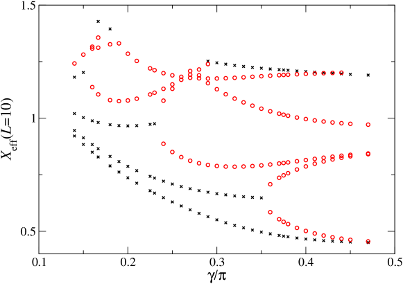
Figure 6: Lowest scaling dimensions (29) in phase III: red circles are derived from the lowest real eigenvalues of (19) for $L=10$, i.e. $20$ lattice sites. Black crosses from the real part of complex eigenvalues.

Moreover, the study of small systems does not yield reliable support for the construction of RG trajectories based our Bethe hypothesis (48) as the root patterns may change drastically when $L$ is varied, see Figure 7.

Figure 7: The left (right) plot displays the dual Bethe-root configuration of the ground state for the phase III in the complex $u$-plane for $2L=10$, ($2L=12$), $\gamma=\frac{\pi}{6}$ and $\alpha=\tfrac{\pi}{2}$.

Based on the diagonalization of the Hamiltonian for system sizes up to $2L\leq 28$ using the Arnoldi-Krylov method Krylov (1931); Arnoldi (1951) we have identified the root configurations for all low energy states. It turns out that only states parameterized by root configurations (48) with quantum numbers $I^{x}_{k}$, $I^{y}_{k}$ shifted against each other are realized on the lattice, e.g.

$$I^{x}_{k} \approx-\frac{M_{x}-1}{2}+\frac{1}{2},-\frac{M_{x}-1}{2}+\frac{3}{2},\dots,+\frac{M_{x}-1}{2}+\frac{1}{2}$$ (51)

$$I^{y}_{k} \approx-\frac{M_{y}-1}{2}-\frac{1}{2},-\frac{M_{y}-1}{2}+\frac{1}{2},\dots,+\frac{M_{y}-1}{2}-\frac{1}{2}$$

$$I^{z}_{k} \approx-\frac{M_{z}-1}{2}-\frac{1}{2},-\frac{M_{z}-1}{2}+\frac{1}{2},\dots,+\frac{M_{z}-1}{2}-\frac{1}{2}$$

for Bethe root configuration displayed in the right panel of Figure 4.

We have investigated the scaling behaviour of such states on the lattice, e.g. the ground state for $L=8$ and its extension to $L=100$ displayed in Figure 8.

Figure 8: Left (right) plot displays the dual Bethe-root configuration of the ground state for $\gamma=\frac{\pi}{6}$, $\alpha=\tfrac{\pi}{2}$ in phase III in the complex $u$-plane for $2L=16$ ($2L=200$).

They show corrections to scaling which increase as $(\log L)^{2}$ with the system size, see Figure 9. This holds also for the imaginary parts of complex energies, such that the appearance of complex energies cannot be argued to be a finite-size effect.

Figure 9: Left (right) plot displays the real (imaginary) part of the effective scaling dimensions of the ground state for $\gamma=\frac{\pi}{6}$ and $\alpha=\frac{\pi}{2}$ as function of the system size $L$. The corresponding root configurations are illustrated in Figure 8. The solid lines are fits to the function $a_{1}+a_{2}\log^{2}(L)+a_{3}L^{-1}$.

This behaviour is a signature of the profound influence of antidiagonal BC on the critical behaviour in the (black hole) phase III. Since a finite study based on the CFT prediction (29) is not possible under such circumstances we have considered the finite size scaling of the energy differences between the ground state and the first excited state, see Figure 10.

Figure 10: The real part of the difference between the effective scaling dimensions of the first excited state and the ground state is shown for $\gamma=\tfrac{\pi}{6}$ and $\alpha=\frac{\pi}{2}$. Left: For large system sizes the gaps close logarithmically, the solid line is a fit to $a_{1}/\log(L)$. Right: For large system sizes (small $B$) the gaps become a linear function of the quasi-momentum (28).

The energy gaps appear to close as $\sim{1}/{L\log(L)}$. Further, the closing of the energy gap seems to be linearly related to the quasi-momentum operator (26). This might signal the remains of the continuous component of the finite-size spectrum observed in phase III for quasi-periodic BC, although the scaling of the ground state is very different. An investigation of this peculiar behaviour in more detail requires an extensive systematic numerical study. As discussed above, such a study faces the difficulty that small $L$ solutions to the Bethe equations often can not be used to seed the corresponding RG-trajectories due to a significant number of level crossings with the system size. Moreover, the construction of the RG-trajectories of these states turns out to be very time-consuming since the root-finding algorithms appear to be extremely sensitive to the initial values. Therefore, we leave the characterization of the scaling limit in this phase as a future research project on its own. Our numerical data for the Bethe root configurations of the ground state and first excitation used in Figures 8, 9 and 10 are available online Frahm and Gehrmann (2024).

Appendix A Matrix elements of the Q-operator

In this appendix, we present our result for the Baxter Q-operator. We have found that the matrix elements of the Q-operator in the tensor product basis $\ket{j}=\ket{\mathbf{s}(j)}=\otimes_{k=1}^{2L}\ket{s_{k}(j)}$, with $s_{k}(j)=\pm 1$ and $\sigma_{k}^{z}\ket{j}=s_{k}(j)\ket{j}$, take the following form

$$\left[\mathbbm{Q}(u)\right]_{i,j}=\frac{Q^{E}_{i,j}(u)}{Q^{E}_{j,j}(u)}\,.$$ (52)

Here $Q^{E}_{i,j}(u)$ has been defined to be

$$Q^{E}_{i,j}(u)=\prod_{k=1}^{2L}h_{k,s_{k}(i)}(\mathbf{s}(j))\,\mbox{e}^{us_{k}(j)/2}\,$$ (53)

where

$$h_{k,s}(\mathbf{t}) =\begin{cases}1&\text{for~{}}s=-1\\ r_{k}(\mathbf{t})\,\mbox{e}^{-ut_{k}}\,\mbox{e}^{\delta_{k}\,t_{k}}&\text{for~{}}s=+1\end{cases}\,,$$

$$r_{k}(\mathbf{t}) =\mbox{e}^{-({\rm i}\gamma/2)\sum_{j=1}^{k}t_{j}}\,\mbox{e}^{({\rm i}\gamma/2)\sum_{j=k+1}^{2L}t_{j}}\,.$$

Note that this implies a normalisation of the Q-operator different from (13), i.e. $\mathbbm{Q}(u\to-\infty)=\mathbbm{1}$ with eigenvalues

$$Q(u)=\prod_{j=1}^{2L}\left(1-\mbox{e}^{u-v_{j}+{\rm i}\gamma/2}\right)\,,$$ (54)

where $v_{j}$ are the Bethe roots solving (15). In this normalisation, the TQ-relation (10) gets modified by two additional phase factors

$$\mathbbm{t}(u)\mathbbm{Q}(u)=\mbox{e}^{{\rm i}L\gamma}\prod^{2L}_{j=1}\sinh(u-\delta_{j}+{\rm i}\gamma)\mathbbm{Q}(u-{\rm i}\gamma)-\mbox{e}^{-{\rm i}L\gamma}\prod^{2L}_{j=1}\sinh(u-\delta_{j})\mathbbm{Q}(u+{\rm i}\gamma)\,.$$ (55)

Let us briefly comment on the relationship to the Q-operator introduced in Ref. Batchelor et al. (1995). While (53) is a straightforward generalisation of the corresponding object in that work to the inhomogeneous case, the expression (52) is new. In Batchelor et al. (1995) the Q-operator satisfying (10) has been defined as $\widetilde{\mathbbm{Q}}(u)=Q^{E}(u)[Q^{E}(u_{0})]^{-1}$, where $Q^{E}$ is the matrix built out of $Q^{E}_{i,j}$ (53) and $u_{0}$ is an arbitrary fixed value of the spectral parameter. Surprisingly, we have found that normalising each matrix element $Q^{E}_{i,j}(u)$ with the associated diagonal elements $Q^{E}_{j,j}(u)$ as in (52) leads to a Q-operator which commutes with itself and the transfer matrix for different values of the spectral parameter and satifies the TQ-relation (55). We have checked this fact numerically for small system sizes. Since (52) does not involve any additional matrix operations on $Q^{E}(u)$ this expression is particularly useful for the numerical computation of the Bethe root configurations.

References

- Jacobsen and Saleur (2006) J. L. Jacobsen and H. Saleur, “The antiferromagnetic transition for the square-lattice Potts model,” Nucl. Phys. B 743, 207 (2006).
- Ikhlef et al. (2008) Y. Ikhlef, J. L. Jacobsen, and H. Saleur, “A staggered six-vertex model with non-compact continuum limit,” Nucl. Phys. B 789, 483 (2008).
- Ikhlef et al. (2010) Y. Ikhlef, J. L. Jacobsen, and H. Saleur, “The staggered vertex model and its applications,” J. Phys. A: Math. Theor 43, 225201 (2010).
- Ikhlef et al. (2012) Y. Ikhlef, J. L. Jacobsen, and H. Saleur, “An integrable spin chain for the SL(2,R)/U(1) black hole sigma model,” Phys. Rev. Lett. 108, 081601 (2012).
- Frahm and Martins (2012) H. Frahm and M. J. Martins, “Phase Diagram of an Integrable Alternating Superspin Chain,” Nucl. Phys. B 862, 504 (2012).
- Candu and Ikhlef (2013) C. Candu and Y. Ikhlef, “Non-Linear Integral Equations for the SL(2,R)/U(1) black hole sigma model,” J. Phys. A: Math. Theor 46, 415401 (2013).
- Frahm and Seel (2014) H. Frahm and A. Seel, “The staggered six-vertex model: Conformal invariance and corrections to scaling,” Nucl. Phys. B 879, 382 (2014).
- Bazhanov et al. (2019) V. V. Bazhanov, G. A. Kotousov, S. M. Koval, and S. L. Lukyanov, “On the scaling behaviour of the alternating spin chain,” JHEP 08, 087 (2019).
- Bazhanov et al. (2021a) V. V. Bazhanov, G. A. Kotousov, S. M. Koval, and S. L. Lukyanov, “Scaling limit of the invariant inhomogeneous six-vertex model,” Nucl. Phys. B 965, 115337 (2021a).
- Kotousov and Lukyanov (2023) G. A. Kotousov and S. L. Lukyanov, “On the scaling behaviour of an integrable spin chain with symmetry,” Nucl. Phys. B 993, 116269 (2023).
- Kotousov and Lukyanov (2021) G. A. Kotousov and S. L. Lukyanov, “ODE/IQFT correspondence for the generalized affine Gaudin model,” JHEP 09, 201 (2021).
- Robertson et al. (2019) N. F. Robertson, J. L. Jacobsen, and H. Saleur, “Conformally invariant boundary conditions in the antiferromagnetic potts model and the sigma model,” JHEP , 10, 254 (2019), arXiv:1906.07565 .
- Robertson et al. (2021) N. F. Robertson, J. L. Jacobsen, and H. Saleur, “Lattice regularisation of a non-compact boundary conformal field theory,” JHEP 02, 180 (2021).
- Frahm and Gehrmann (2022) H. Frahm and S. Gehrmann, “Finite size spectrum of the staggered six-vertex model with -invariant boundary conditions,” JHEP 01, 70 (2022).
- Frahm et al. (2023) H. Frahm, S. Gehrmann, and G. A. Kotousov, “Scaling limit of the staggered six-vertex model with invariant boundary conditions,” preprint (2023), 10.48550/arXiv.2312.11238.
- Frahm and Gehrmann (2023) H. Frahm and S. Gehrmann, “Integrable boundary conditions for staggered vertex models,” J. Phys. A: Math. Theor 56, 025001 (2023).
- Yung and Batchelor (1995) C. M. Yung and M. T. Batchelor, “Exact solution for the spin- XXZ quantum chain with non-diagonal twists,” Nucl. Phys. B 446, 461 (1995).
- Batchelor et al. (1995) M. T. Batchelor, R. J. Baxter, M. J. O’Rourke, and C. M. Yung, “Exact solution and interfacial tension of the six-vertex model with anti-periodic boundary conditions,” J. Phys. A: Math. Gen. 28, 2759 (1995).
- von Gehlen et al. (1988) G. von Gehlen, V. Rittenberg, and G. Schütz, “Operator content of -state quantum chains in the region,” J. Phys. A: Math. Gen. 21, 2805 (1988).
- Alcaraz et al. (1988) F. C. Alcaraz, M. Baake, U. Grimmn, and V. Rittenberg, “Operator content of the XXZ chain,” J. Phys. A: Math. Gen. 21, L117 (1988).
- Niekamp et al. (2009) S. Niekamp, T. Wirth, and H. Frahm, “The XXZ model with anti-periodic twisted boundary conditions,” J. Phys. A: Math. Theor 42, 195008 (2009).
- Baxter (1972) R. J. Baxter, “Partition function of the eight-vertex lattice model,” Annals of Physics 70, 193 (1972).
- Sklyanin (1985) E. K. Sklyanin, “The Quantum Toda Chain,” Springer: Lect. Notes in Phys. 226, 196 (1985).
- Sklyanin (1992) E. K. Sklyanin, “Quantum Inverse Scattering Method. Selected Topics,” World Scientific: Nankai Lect. in Math. Phys. , 63 (1992).
- Bazhanov et al. (2021b) V. V. Bazhanov, G. A. Kotousov, S. M. Koval, and S. L. Lukyanov, “Some algebraic aspects of the inhomogeneous six-vertex model,” SIGMA 17, 025 (2021b).
- Robertson et al. (2020) N. F. Robertson, M. Pawelkiewicz, J. L. Jacobsen, and H. Saleur, “Integrable boundary conditions in the antiferromagnetic Potts model,” JHEP 05, 144 (2020).
- Polyakov (1970) A. M. Polyakov, “Conformal symmetry of critical fluctuations,” JETP Lett 12, 381 (1970).
- Cardy (1986) J. L. Cardy, “Operator content of two-dimensional conformally invariant theories,” Nucl. Phys. B 270, 186 (1986).
- Bloete et al. (1986) H. W. J. Bloete, J. L. Cardy, and M. P. Nightingale, “Conformal invariance, the central charge and universal finite-size amplitudes at criticality,” Phys. Rev. Lett. 56, 742 (1986).
- Yang and Yang (1969) C. N. Yang and C. P. Yang, “Thermodynamics of a one-dimensional system of bosons with repulsive delta-function interaction,” J. Math. Phys. 10, 1115 (1969).
- Krylov (1931) A. N. Krylov, “On the numerical solution of the equation by which the frequency of small oscillations is determined in technical problems,” Izv. Akad. Nauk SSSR, Ser. Fiz.-Mat. , 491 (1931).
- Arnoldi (1951) W. E. Arnoldi, “The principle of minimized iterations in the solution of the matrix eigenvalue problem,” Q. Appl. 8, 17 (1951).
- Frahm and Gehrmann (2024) H. Frahm and S. Gehrmann, “Dataset: Bethe ansatz data for the staggered six-vertex model with antidiagonal boundary conditions ,” https://doi.org/10.25835/hl5nqg81 (2024), Research Data Repository, Leibniz Universität Hannover.