Transportation Science

Hagn et al.

Stochastic Team Formation and Routing

A Branch-Price-Cut-And-Switch Approach for Optimizing Team Formation and Routing for Airport Baggage Handling Tasks with Stochastic Travel Times

Andreas Hagn Technical University of Munich, TUM School of Management, Department of Operations & Technology
AdONE GRK 2201
andreas.hagn@tum.de Rainer Kolisch Technical University of Munich, TUM School of Management, Department of Operations & Technology
rainer.kolisch@tum.de Giacomo Dall’Olio Technical University of Munich, TUM School of Management, Department of Operations & Technology
AdONE GRK 2201
giacomo.dallolio@tum.de Stefan Weltge Technical University of Munich, TUM School of Computation, Information and Technology
Department of Discrete Mathematics
weltge@tum.de

In airport operations, optimally using dedicated personnel for baggage handling tasks plays a crucial role in the design of resource-efficient processes. Teams of workers with different qualifications must be formed, and loading or unloading tasks must be assigned to them. Each task has a time window within which it can be started and should be finished. Violating these temporal restrictions incurs severe financial penalties for the operator. In practice, various components of this process are subject to uncertainties. We consider the aforementioned problem under the assumption of stochastic travel times across the apron. We present two binary program formulations to model the problem at hand and solve it with a Branch-Price-Cut-and-Switch approach, in which we dynamically switch between two master problem formulations. Furthermore, we use an exact separation method to identify violated rank-1 Chvátal-Gomory cuts and utilize an efficient branching rule relying on task finish times. We test the algorithm on instances generated based on real-world data from a major European hub airport with a planning horizon of up to two hours, 30 flights per hour, and three available task execution modes to choose from. Our results indicate that our algorithm is able to significantly outperform existing solution approaches. Moreover, an explicit consideration of stochastic travel times allows for solutions that utilize the available workforce more efficiently, while simultaneously guaranteeing a stable service level for the baggage handling operator.

airport operations, team formation, routing, hierarchical skills, uncertainty, branch-price-and-cut

1 Introduction

Baggage handling tasks, namely loading and unloading containers and bulk luggage, play an important role in aviation and airport operations. They are one of several ground handling tasks (Evler et al. (2021)). Whenever a plane is arriving or scheduled for departure, a team of workers that operates several types of equipment needs to be formed and assigned to load or unload the aircraft. Said workers have different skill levels, i.e., qualifications for the types of equipment, such as tractors or high cargo loaders, they are allowed to operate. Depending on the airplane model and type, various equipment compositions can be used to execute the (un-)loading task, leading to different workforce requirements. For instance, large-sized airplanes typically have at least two cargo holes. These can be unloaded either sequentially or in parallel. For a more detailed description of the processes, see Dall’Olio and Kolisch (2023). In the following, whenever loading tasks are discussed, both loading and unloading processes are encompassed.
Each type of equipment requires a certain skill level, where skill levels are ordered hierarchically. That is, a worker with skill level $k$ can execute any job requiring a skill level of $k$ or lower. Frequent delays in baggage claim processes and plane departures can result from improper team formation and task assignment decisions. This noticeably decreases passenger satisfaction and induces significant financial penalties for the baggage handling operator. In practice, both loading times and travel times between parking positions vary heavily. Delays while traveling from one parking position to another, e.g., because of planes crossing the apron, are quite frequent and typically accumulate to a significant scope. In the following, we consider loading times to be deterministic, while travel times are assumed to be stochastic with known probability distributions. Moreover, to limit the potential financial penalties for the baggage handling operator, it is reasonable to demand that each task’s time window is satisfied with at least a predefined probability. Our work builds upon Dall’Olio and Kolisch (2023), which addresses the deterministic team formation and routing problem. The main contributions of this paper are:

• We extend previous works on baggage handling optimization by including stochastic travel times.

• We propose a novel Branch-Price-Cut-and-Switch solution approach that dynamically switches between two master problem formulations, depending on the solution’s characteristics.

• We conduct extensive experimental studies to analyze the impact of stochastic information on optimal solutions and assess our solution method’s efficiency.

The remainder of this paper is structured as follows. Section 2 reviews the most relevant literature for our study. Section 3 provides a detailed problem description with the help of mathematical notation. In Section 4, we propose two binary programs that are used to model the problem at hand. In Section 5, we develop a Branch-Price-Cut-and-Switch solution approach and elaborate on its core components. Section 6 presents computational experiments aiming at assessing the proposed algorithm’s performance and the impact of stochasticity on optimal solutions. We summarize our findings in Section 7 and present several areas of future research.

2 Literature Review

The problem considered in this paper can be seen as a variant of the technician scheduling and routing problem (TSRP). TSRPs typically consist of a routing part that can be seen as a vehicle routing problem (VRP) and a scheduling or team formation part. Section 2.1 focuses on literature dealing with stochastic VRPs in a general context. Section 2.2 consolidates publications dealing with stochastic TSRP variants.

2.1 Literature on Stochastic Vehicle Routing

Recently, stochastic formulations of the vehicle routing problem with time windows (VRPTW) have seen a noticeable increase in interest. In the following, we provide an overview of literature dealing with stochastic variants of the VRPTW. Oyola, Arntzen, and Woodruff (2018) summarize the most relevant literature on common types of stochastic VRPs. A taxonomy and overview of the space of VRPs can be found in Eksioglu, Vural, and Reisman (2009).
Generally, random variables in the stochastic VRPTW are assumed to be independent as stochastic dependency drastically complicates the calculation of distributions and their moments. While some publications focus on the VRPTW with stochastic demands (see Lee, Lee, and Park (2012), Zhang, Lam, and Chen (2016)), stochastic travel and service times are far more common. Stochasticity can be addressed in different ways. A common approach is to include chance constraints, which limit the probability of violating time windows. While Errico et al. (2018) connect chance constraints to the simultaneous satisfaction of all time windows, Ehmke, Campbell, and Urban (2015) as well as Li, Tian, and Leung (2010) limit the probability of violating the time window of each customer individually.
Furthermore, time windows can either be hard or soft, i.e., services may or may not be allowed to start before the time window opens or after it closes. Taş et al. (2014) assume that travel times are stochastically independent, gamma distributed random variables, and time windows are soft. The authors propose an exact calculation of arrival time distributions by convolving finish time and travel time distributions and solve the problem using a Branch-Price-and-Cut approach.
If time windows are assumed to be hard, arrival time distributions need to be truncated at the start of each time window. Hence, distributional structures are not propagated along vehicle routes, often making an exact calculation of distributions impossible. Errico et al. (2018) assume service times to be stochastic, discretely distributed random variables and calculate start time distributions exactly. They use a Branch-Price-and-Cut algorithm to solve the problem and report computational results for four different types of travel time distributions. Miranda and Conceição (2016) assume normally distributed service and travel times and approximate start time distributions by discretizing the start time distribution at the previous task on intervals of dynamic length. They further improve their approach in Miranda, Branke, and Conceição (2018) by using better lower bounds for service and travel times. Ehmke, Campbell, and Urban (2015) show that the first and second moment of start time distributions can be calculated with little effort if both travel times and start times at the previous task are normally distributed. While the former is usually not the case, the authors present computational results that indicate that their approach works well for normal, shifted gamma, and shifted exponential travel time distributions. Li, Tian, and Leung (2010) use stochastic simulation to derive estimates for start time distributions and solve the problem using tabu search.
Our considerations can be seen as a combination and extension of Errico et al. (2018) and Li, Tian, and Leung (2010), as we calculate start time distributions exactly but interpret chance constraints as a non-route-interdependent property and consider a stochastic objective function.

2.2 Literature on the stochastic TSRP

Unlike for the vehicle routing problem, there is no standard definition for the TSRP. In general, the TSRP consists of scheduling workers or assembling teams of workers and routing them across available tasks such that each task is executed by exactly one team (or worker). Depending on the context, additional requirements must be considered.
We first focus on literature on deterministic variants of the TSRP that share several key properties with the problem at hand. Pereira, Alves, and de Oliveira Moreira (2020) consider a multiperiod workforce scheduling and routing problem, where tasks do not have a fixed time window. However, precedence relationships need to be satisfied. The set of available teams and their characteristics, such as skill levels, are fixed and thus are not part of the decision space. The authors propose a mixed-integer model, which is shown to be computationally tractable only for small instances, and an ant-colony optimization heuristic. Çakırgil, Yücel, and Kuyzu (2020) examine a multi-objective workforce scheduling and routing problem, where teams consisting of workers with different skills need to be formed and task sequences need to be assigned to each team. Tasks can be started at any time, but need to be finished before their respective deadline. Workers can have different qualifications, but it is not possible for them to execute tasks that require a different qualification, i.e., downgrading is not possible. The authors developed a mixed-integer program and a 2-stage matheuristic to solve the problem. While the former proves to be inefficient for large instances, the latter is able to scale well with instance size. Li, Lim, and Rodrigues (2005) consider a manpower allocation problem with hard time windows. Similar to Çakırgil, Yücel, and Kuyzu (2020), workers with different qualifications need to be grouped into teams, which then execute a to-be-optimized sequence of tasks. Additionally, downgrading workers is not possible. The objective is to minimize a weighted sum of the total number of required workers and the total travel time. The authors develop a construction heuristic and a simulated annealing approach to solve the problem.
All of the publications previously discussed differ from our considerations in two aspects. First, they fix teams beforehand or make restrictive assumptions regarding team formation possibilities, such as the impossibility of downgrading or the existence of a single mode. Second, they focus on heuristic solution methods to solve medium- and large-sized instances. For an overview of further literature dealing with deterministic variants of the TSRP relevant to this study, the interested reader is referred to Dall’Olio and Kolisch (2023).
While there is plenty of literature regarding the deterministic TSRP, very little research has been done on stochastic problem variants. In the following, we turn our focus on literature dealing with stochastic variants of the TSRP that are similar to ours.
Souyris et al. (2013) propose a robust formulation for the TSRP. Workers are assumed to be homogeneous and service times are stochastic. Each task must be started before a fixed deadline with a given probability. Moreover, each task must be executed by a single technician, thus team formation is not part of the model. The authors propose three different bounded uncertainty sets that limit the total service time delays per technician or client, respectively. The objective is to minimize the worst-case total delay and travel time. A branch-and-price approach is proposed and applied to real-world instances with 41 customers and 15 technicians.
Yuan, Liu, and Jiang (2015) address the TSRP in the context of health care workers and home health care services. Each task must be executed by a single worker. Furthermore, it is possible to downgrade workers to lower skill levels. Service times are assumed to be stochastic with a known probability distribution. To mitigate the need for explicitly calculating start time distributions, a scenario-based approach is presented. The goal is to minimize the expected total travel costs, fixed costs of caregivers, service costs, and penalties for late arrival at customers. The authors use a branch-and-price approach to solve the problem exactly. Computational experiments assuming uniformly distributed service times and 25 to 50 customers indicate that the approach is able to provide very good results for small-sized instances.
Binart et al. (2016) consider a TSRP with mandatory and optional tasks, where time windows are hard and fixed, predefined teams can be used to execute tasks. Although not explicitly done, their modeling framework would allow considering multiple skill levels, downgrading, and multiple modes for single tasks. The authors assume that travel and service times are discretely distributed according to triangular distributions. Furthermore, the time windows of each task must be satisfied with a given probability. A 2-stage approach is proposed to heuristically solve the problem. First, a feasible skeleton solution is obtained using a generic MIP solver by optimally covering all mandatory tasks. Second, the first-stage solution is refined by inserting optional customers into the existing routes such that time window restrictions are not violated. Computational results on instances with 5 to 9 mandatory and 30 to 50 optional tasks indicate that the approach can yield good results in most cases.
Our work shows several similarities with Binart et al. (2016) and Yuan, Liu, and Jiang (2015), such as the stochasticity of travel times, the usage of an exact solution method, and the incorporation of several team properties such as multiple skill levels and modes. At the same time, our interpretation of service levels at individual tasks rather than entire solutions, the lack of assumptions on distributional properties, and the exact calculation of arrival times separate our considerations from previous approaches.
To conclude this section, it is worth noting that existing research primarily deals with heuristic solution procedures. Exact approaches are typically only efficient for small-sized instances, especially when stochasticity is considered.

3 Problem Description

In the following section, we provide a detailed description of the problem considered in this publication with the help of mathematical notation, which will be used throughout the following sections.

General Notation

We consider a set $\mathcal{I}=\{1,\dots,|\mathcal{I}|\}$ of tasks that have to be performed within a specified planning horizon. Each task corresponds to either a loading or unloading task of an incoming (or outgoing) flight. A time window $[ES_{i},LF_{i}]$ is associated with each task $i\in\mathcal{I}$, describing the earliest and latest point at which service on an airplane can be started and should be finished, respectively.
Initially, a workforce of prespecified size is located at a central depot denoted by $d$. In general, workers can be subdivided into skill levels $\mathcal{K}\coloneqq\{1,\dots,K\}$. Depending on their skill level, workers are only allowed to operate certain equipment. Skill levels are ordered hierarchically, i.e., a worker with level $k$ is able to operate any equipment requiring level $l\leq k$. Moreover, the amount of workers with skill level $\geq k$ that are available for disposition is fixed and defined as $N_{k}\coloneqq\underset{\kappa=k}{\overset{K}{\sum}}N_{k}^{D}$, where $N_{k}^{D}\in\mathbb{N}_{>0}$ is the number of available workers with skill level $k$. We note that in practical instances, higher-skilled workers tend to be rather scarce and hard to obtain as they require lengthy and expensive training. A route is a sequence $r\coloneqq\left(d,v_{1},\dots,v_{l},d\right)$ with $l\geq 1$ and $v_{i}\in\mathcal{I}$ for all $i=1,\dots,l$. Each route $r$ has time instants $tl^{r}$ and $tr^{r}$ at which the team leaves the depot and returns to it, respectively. The set of tasks executed by route $r$ is denoted by $\mathcal{I}^{r}\coloneqq\{v_{1},\dots,v_{l}\}$. Furthermore, each route $r$ is assigned a profile $q=\left(\xi_{q,k}\right)_{k\in\mathcal{K}}\in\mathcal{Q}$ which is used to execute the route, where $\xi_{q,k}\in\mathbb{N}_{\geq 0}$ denotes the number of required workers of skill level greater than or equal to $k$ and $\mathcal{Q}$ is the set of available profiles. Because each type of aircraft requires different prerequisites and equipment for baggage handling tasks, only a subset $\mathcal{Q}_{i}\subseteq\mathcal{Q}$ of profiles can be used to execute a given task $i\in\mathcal{I}$. Depending on the profile $q\in\mathcal{Q}_{i}$, executing task $i$ takes $p_{i,q}\in\mathbb{N}_{>0}$ units of time.

Profiles and Skill Compositions

By construction, a profile $q\in\mathcal{Q}$ is well-defined by its aggregated workforce requirements, i.e., lower bounds on the skill levels of required workers, but does not contain any information about their actual skill levels. To include this information, we define a skill composition as a vector $s\in\mathbb{N}^{|\mathcal{K}|}$ and say that a skill composition $s=(s_{q,k})_{k\in\mathcal{K}}$ be can assigned to a profile $q\in\mathcal{Q}$ if

$$\xi_{q,k^{*}} =\underset{k\in\mathcal{K}}{\sum}s_{q,k}\quad\text{and}$$ (1)

$$\xi_{q,k^{\prime}} \leq\underset{k\in\mathcal{K}:k\geq k^{\prime}}{\sum}s_{q,k}\quad\forall k^{\prime}\in\mathcal{K}$$ (2)

hold, where $k^{*}=1$ is the skill level with the lowest qualification. Furthermore, the set

$$\mathcal{S}_{q}\coloneqq\left\{(s_{q,k})_{k\in\mathcal{K}}:\ (s_{q,k})_{k\in\mathcal{K}}\ \text{satisfies}\ (\ref{definition_skill_comp_sum})-(\ref{definition_skill_comp_leq})\right\}$$

consists of all skill compositions that can be assigned to profile $q\in\mathcal{Q}$. Hence, we define the set

$$\mathcal{Q}^{D}\coloneqq\left\{(q,s):q\in\mathcal{Q},s\in\mathcal{S}_{q}\right\}.$$

as the set of disaggregated profiles, i.e., profiles enhanced by information on the skill levels of workers used to assemble a team with profile $q$. Given a route $r$, we define the set of profiles that can be used to execute $r$ as $\mathcal{Q}^{r}\coloneqq\underset{i\in\mathcal{I}^{r}}{\bigcap}\mathcal{Q}_{i}$. An example illustrating the relationship between profiles and skill compositions is presented in Section 4.2.

Travel Times

After finishing a task $i$, a team with profile $q$ can either return to the depot $d$ and become available for regrouping or directly continue with another task $j$. Traveling between locations $i,j\in\mathcal{I}\cup\left\{d\right\}$, where $i$ and $j$ are either two tasks or one task and the depot, takes at least $t_{i,j}^{det}\in\mathbb{N}_{\geq 0}$ units of time and does not depend on the profile. We note that we assume travel times to be symmetric and time-independent. In practice, these travel times are subject to delays caused by unexpected, exogenous factors, such as aircrafts crossing the apron or local traffic congestions. To formalize this, we define non-negative, finite supports for travel time delays for each pair $(i,j)$ of tasks (or tasks and the depot) by

$$B_{i,j}\subset\mathbb{N}_{\geq 0},\ |B_{i,j}|<\infty\quad\forall(i,j)\in E$$

where $E\coloneqq\left\{(i,j):i,j\in\mathcal{I}\cup\{d\},\ i\neq j\right\}$. We then define the set of possible travel time delays by

$$\Omega\coloneqq\underset{(i,j)\in E}{\bigtimes}B_{i,j}.$$

Then, the vector of stochastic travel times $t:\ \Omega\rightarrow\mathbb{N}_{>0}^{|E|}$ is given by

$$t(\omega) =t^{det}+\omega\quad\forall\omega\in\Omega$$

for all $(i,j)\in E$. Consistently, we can represent $t(\omega)$ as $t(\omega)=(t_{i,j}(\omega))_{(i,j)\in E}=(t_{i,j}^{det}+\omega_{i,j})_{(i,j)\in E}$. We assume that events in $\Omega$ are stochastically independent, thus $(t_{i,j})_{(i,j)\in E}$ are stochastically independent, non-negative random variables with finite support. In the following, $t_{i,j}^{det}$ is also called deterministic or best-case travel time. Additionally, we denote the worst-case scenario of travel times by

$$\omega_{max}=\left(\max\{\omega_{i,j}:\omega_{i,j}\in B_{i,j}\}\right)_{(i,j)\in E}$$

Routes and Route Feasibility

If a worker team arrives at task $i$ before its time window opens, it has to wait until $ES_{i}$ to start the service. Because travel times are stochastic, the start and finish times $S_{i}^{r,q}$ and $F_{i}^{r,q}\coloneqq S_{i}^{r,q}+p_{i,q}$ of a task $i$ executed by a team with profile $q$ within route $r$ are also stochastic. As the actual travel times are random and hardly predictable beforehand, finishing tasks after the time window closes, i.e., after $LF_{i}$, is sometimes inevitable. At the same time, this incurs high fines for the baggage task operator and reduces passenger satisfaction. Therefore, we allow tasks to be finished after their time window closes, while we limit said violation to at most a fixed amount of time, leading to a new extended latest finish time $LF_{i}^{e}\geq LF_{i}$ for each task $i$. Furthermore, to limit potential financial damages and customer dissatisfaction, we introduce a minimum service level $\alpha\in[0,1]$ and demand that the finish time $F_{i}^{r,q}$ of each task $i$ on each route $r$ must satisfy

$$\mathbb{P}(F_{i}^{r,q}\leq LF_{i})\geq\alpha,$$ (3)

$$\mathbb{P}(F_{i}^{r,q}>LF_{i}^{e})=0.$$ (4)

Constraint (3), also called chance constraint or service level constraint, limits the probability of delays caused by the baggage handling operator, while constraint (4) guarantees that potential delays do not exceed a prespecified limit. A route $r$ with profile $q$ is called feasible if (3)–(4) are satisfied for all $i\in\mathcal{I}^{r}$.

Route Costs and Objective Function

Each task $i\in\mathcal{I}$ has an assigned weight $w_{i}\geq 0$ that indicates its importance in the flight schedule. This can be, for instance, the number or percentage of passengers that have to reach a connecting flight at the destination airport. The expected cost of a route $r$ with profile $q$ is then given by

$$\mathbb{E}(c^{r})=\underset{i\in\mathcal{I}^{r}}{\sum}w_{i}\cdot\mathbb{E}\left(\left(F_{i}^{r,q}-EF_{i}\right)+P_{i}(F_{i}^{r,q})\right)$$

where $EF_{i}\coloneqq ES_{i}+\min\{p_{i,q}:\ q\in\mathcal{Q}_{i}\}$ is the earliest possible finish time of task $i$ and $P_{i}:(LF_{i},LF_{i}^{e}]\rightarrow\mathbb{R}_{>0}$ is a penalty function. The first part of the objective functions aims to minimize weighted expected finish times in order to have as large safety time buffers as possible to absorb delays in other parts of the baggage handling process. The second part consists of a penalty for delaying flights. Because delaying a single flight by a larger amount of time is considered more severe than delaying multiple flights only slightly, we use a quadratic penalty function

$$P_{i}(F_{i}^{r,q}(\omega))\coloneqq\begin{cases}(F_{i}^{r,q}(\omega)-LF_{i})^{2}&F_{i}^{r,q}>LF_{i},\\ 0&\text{else}\end{cases}$$

for all $\omega\in\Omega$. In order to calculate the expected cost of a route $r=(d,v_{1},\dots,v_{l},d)$ with $l\geq 1$, it is necessary to have full information about the finish time distribution of each task assigned to $r$. Let $i,j\in\mathcal{I}$ be two tasks that are executed consecutively in route $r$, i.e., there exists an $h\in\{1,\dots,l-1\}$ with $v_{h}=i$ and $v_{h+1}=j$. If the distribution of $F_{i}^{r,q}$ is known, the start time distribution of the subsequent task $S_{j}^{r,q}$ can be calculated as

$$\mathbb{P}(S^{r,q}_{j}=\tau)=\begin{cases}\underset{z=0}{\overset{ES_{j}}{\sum}}\mathbb{P}(F^{r,q}_{i}+t_{i,j}=z)&\tau=ES_{j}\\ \mathbb{P}(F^{r,q}_{i}+t_{i,j}=\tau)&\tau>ES_{j}\\ 0&\text{else}\end{cases}$$ (5)

The finish time distribution $F_{j}^{r,q}$ can then be obtained by using that $F_{j}^{r,q}=S_{j}^{r,q}+p_{j,q}$ holds by definition.

4 Two Binary Program Formulations

In the following sections, we present two set-covering formulations for the problem. In Section 4.1, we extend the model proposed in Dall’Olio and Kolisch (2023) to incorporate stochastic travel times and a stochastic objective function. As this model considers the workforce only on an aggregated level, we might obtain an integer solution that is operationally infeasible, i.e., it can not be implemented in practice. Whenever such a solution is found, we switch to an alternative formulation that considers workers based on individual skill levels. This alternative formulation, which always returns operationally feasible solutions but is considerably harder to solve, is presented in Section 4.2, alongside additional insights into operational feasibility.

4.1 Master Problem with Aggregated Workforces

The following considerations assume an underlying finite time grid given by discrete time points $\tau\in\mathcal{T}$. We first introduce general notation and several auxiliary parameters. We define a team route as a tuple $(r,q)$ consisting of a feasible route $r$ and an associated worker profile $q\in\mathcal{Q}^{r}$, which is used to execute the route. The set of team routes is denoted by $\mathcal{R}$.
Given a realization $\omega\in\Omega$ of travel times, the start and finish times of a task $i\in\mathcal{I}^{r}$ are then defined by

$$S_{i}^{r,q}(\omega) \coloneqq\max\{F_{i-1}^{r,q}(\omega)+t_{i-1,i}(\omega),ES_{i}\}\quad\text{and}$$

$$F_{i}^{r,q}(\omega) \coloneqq S_{i}^{r,q}(\omega)+p_{i,q}$$

where $F_{d}^{r,q}(\omega)=tl^{r}$ is equal to the depot leave time of route $r$ and $i-1$ is the predecessor of task $i$ along $r$. Furthermore, we denote by $tr^{r}$ the worst-case return time of route $r$, which is realized whenever the worst-case scenario $\omega_{max}$ occurs.
Let $(r,q)\in\mathcal{R}$ be a team route. We define by $b_{k,\tau}^{q}(\omega_{max})\in\mathbb{N}_{\geq 0}$ the number of workers of skill level $\leq k$ that are conducting route $r$ and are occupied at time $\tau$, given worst-case travel times $t(\omega_{max})$. This value is equal to $\xi_{q,k}$ for all $\tau\in[tl^{r},tr^{r}]$ and $0$ else. Binary variables $\lambda^{r}_{q}$ indicate if team route $(r,q)$ is part of the solution. The problem can then be described using the following aggregated master problem, short AMP:

$$\min \sum_{(r,q)\in\mathcal{R}}\mathbb{E}(c^{r})\lambda^{r}_{q}$$ (6)

s.t. $$\underset{(r,q)\in\mathcal{R}:\ i\in\mathcal{I}^{r}}{\sum}\lambda^{r}_{q}\geq 1\quad\forall i\in\mathcal{I}$$ (7)

$$\underset{(r,q)\in\mathcal{R}}{\sum}b_{k,\tau}^{q}(\omega_{max})\lambda^{r}_{q}\leq N_{k}\quad\forall k\in\mathcal{K},\ \forall\tau\in\mathcal{T}$$ (8)

$$\lambda^{r}_{q}\in\{0,1\}\quad\forall(r,q)\in\mathcal{R}$$ (9)

Constraints (7) ensure that each task is part of at least one route. It is easy to see that covering a task more than once can not be part of an optimal solution. Inequalities (8) guarantee that the workforce required at any given time $\tau$ does not exceed the total available workforce on an aggregate level. The objective function (6) aims to minimize the expected finish times of tasks and incurred penalties in order to maximize buffer times. Furthermore, the AMP with only a subset of team routes $\bar{\mathcal{R}}\subset\mathcal{R}$ considered and binary conditions (9) relaxed to $\lambda^{r}_{q}\in[0,1]$ is called aggregated reduced master problem (ARMP). However, for the sake of simplicity, we will still be referring to the set of columns of the ARMP as $\mathcal{R}$.
We note that chance constraints (3) are not route-interdependent, thus they can be fully embedded in the pricing problem.

4.2 Master Problem with Skill-Level Specific Workforces

In the following, we provide a more detailed master problem that considers the workforce on an individual skill level basis. Furthermore, we provide some insights into the dominance relation between the two proposed master problem formulations.
Let $(r,q)\in\mathcal{R}$ be a team route. As described in Section 3, $q$ is well-defined by the amount $\xi_{q,k}$ of required workers of skill level greater or equal than $k$ for all $k\in\mathcal{K}$. This information suffices to ensure that the available workforce is never exceeded on an aggregate level, but does not guarantee feasibility in terms of allocation of workers to individual tasks. For an example, the interested reader is referred to Section 4.2 of Dall’Olio and Kolisch (2023).
To deal with such undesirable solutions, the aforementioned authors propose an integer problem called feasibility check, which tries to find a feasible allocation of available workers to teams and regrouping strategies by solving a network flow problem on an appropriate graph. If said problem is infeasible, a cut is added to the master problem and the ARMP is re-solved. In preliminary studies, we observed that there are several instances in which a large number of cuts have to be added, degrading the algorithm’s performance by a large margin. In such instances, there is a large cardinality of binary solutions to the ARMP that all share the property of being operationally infeasible in the previously described sense and have the same (or almost the same) objective function value. This makes it necessary to consecutively forbid these solutions one by one, which in turn makes the master problem computationally harder as each additional cut increases the pricing step’s complexity. Additionally, the ARMP has to be re-solved every time without improving the solution quality.
We mitigate this issue by utilizing the concept of skill compositions to develop an alternative formulation to the AMP. For this, we define a disaggregated team route $(r,q,s)$ as a tuple consisting of a team route $(r,q)\in\mathcal{R}$ and a disaggregated profile $(q,s)\in\mathcal{Q}^{D}$ and denote the set of disaggregated team routes by $\mathcal{R}^{D}$.

Example 4.1

Consider the following example of a team route $(r,q)\in\mathcal{R}$ with $r\in\mathcal{R}$, $q\in\mathcal{Q}^{r}$ . We define $\mathcal{K}\coloneqq\{1,2,3\}$ and profile $q$ by

$$b_{\tau}^{q}(\omega_{max})\coloneqq\left(b_{i,\tau}^{q}(\omega_{max})\right)_{i=1,2,3}=\left(\begin{array}[]{c}3\\ 2\\ 1\\ \end{array}\right)$$

for $\tau\in[tl^{r},tr^{r}]$. Furthermore, we assume that we have an unlimited workforce available for each skill level.

Table 1: Set of possible skill compositions for profile $q$

Profile Skill compositions k $b^{q}_{k,\tau}(\omega_{max})$ $\beta^{q}_{k,\tau}(\omega_{max})$ 1 3 1 0 0 1 0 2 2 1 2 1 0 0 3 1 1 1 2 2 3

There are multiple skill compositions $\left(\beta^{s}_{k,\tau}(\omega_{\max})\right)_{i=1,2,3}$ that can be used to assemble a team with profile $q$, which are visualized in Table 1. In total, team route $(r,q)$ can be used to derive five unique team routes in $\mathcal{R}^{D}$. For instance, the second column in Table 1 implies the usage of two workers of level 2 and one worker of level 3 to assemble a team with profile $q$.

We use these concepts to develop a model analogous to the AMP. For each $(r,q,s)\in\mathcal{R}^{D}$, we define by $\beta_{k,\tau}^{s}(\omega_{max})$ the number of workers of skill level $k$ required by route $r$ at time $\tau$, assuming worst-case travel times. These parameters take values $\beta_{k,\tau}^{s}=s_{q,k}$ for $\tau\in[tl^{r},tr^{r}]$ and $\beta_{k,\tau}^{s}=0$ otherwise. Using the previous definitions, we introduce the disaggregated master problem, abbreviated as DMP:

$$\min \sum_{(r,q,s)\in\mathcal{R}^{D}}\mathbb{E}(c^{r})\lambda^{r}_{q,s}$$ (10)

s.t. $$\underset{(r,q,s)\in\mathcal{R}^{D}:\ i\in\mathcal{I}^{r}}{\sum}\lambda^{r}_{q,s}\geq 1\quad\forall i\in\mathcal{I}$$ (11)

$$\underset{(r,q,s)\in\mathcal{R}^{D}}{\sum}\beta_{k,\tau}^{s}(\omega_{max})\lambda^{r}_{q,s}\leq N_{k}^{D}\quad\forall k\in\mathcal{K},\ \forall\tau\in\mathcal{T}$$ (12)

$$\lambda^{r}_{q,s}\in\{0,1\}\quad\forall(r,q,s)\in\mathcal{R}^{D}$$ (13)

Unlike in Section 4.1, constraints (12) consider workforces on an individual rather than an aggregated level. Similar to the ARMP, we call the DMP when only a subset of routes is considered and (13) is replaced by $\lambda^{r}_{q,s}\in[0,1]$ the aggregated reduced master problem (ARMP). For ease of reading, we will be referring to the columns of the DRMP as the set $\mathcal{R}^{D}$. Moreover, we denote a solution $(\hat{\lambda}^{r}_{q})_{(r,q)\in\mathcal{R}}$ to the ARMP, which can not be extended to a solution $(\hat{\lambda}^{r}_{q,s})_{(r,q,s)\in{\mathcal{R}^{D}}}$ of the DRMP as a disaggregated-infeasible solution. We note that this can be checked by solving the feasibility check, which has been proposed by Dall’Olio and Kolisch (2023) and is included in Appendix 9 of this publication.
Each disaggregated team route $(r,q,s)\in\mathcal{R}^{D}$ corresponds to one column of the DRMP. It is easy to see that $|\mathcal{R}^{D}|$ is considerably larger than $|\mathcal{R}|$. A formal proof of this is provided in Appendix LABEL:appendix_dominance_dmp. Additionally, each column in $\mathcal{R}$ can be obtained by convex combinations of columns in $\mathcal{R}^{D}$. Thus, vertices of the feasible region of the linear relaxation of the ARMP may correspond to higher-dimensional faces in the DRMP. This makes it significantly harder to cut off non-integer solutions from the feasible region; therefore, solving the DRMP using a branch-and-cut algorithm becomes substantially harder. Experimental studies have shown that solving the DRMP is, on average, around 30% slower than solving the ARMP. Therefore, we only resort to solving the DRMP once a disaggregated-infeasible solution has been identified.

5 Solution Approach

In this section, we present a Branch-Price-Cut-and-Switch algorithm to solve the problem at hand. We initially start the algorithm at the root node with a subset of columns, denoted by $\bar{\mathcal{R}}\subset\mathcal{R}$, consisting of single-task tours $(d,i,d)$ for each task $i\in\mathcal{I}$, each profile $q\in\mathcal{Q}_{i}$ and the earliest possible depot leave time $tl\coloneqq ES_{i}-t_{d,i}(\omega_{max})$. To ensure feasibility, we include a column that finishes each task at the latest possible time $LF_{i}^{e}$ and uses up the entire available workforce. We then search the branching tree using a Branch-Price-and-Cut approach. If we obtain an integer solution, we perform the feasibility check proposed by Dall’Olio and Kolisch (2023) to check if the solution is disaggregated-feasible. If the solution fails the feasibility check, we mark the current node and its sibling node as disaggregated-infeasible and restart the procedure. We note that children of marked nodes are also marked by default. Whenever a disaggregated-infeasible node is encountered with the search tree, we solve the DRMP instead of the ARMP. The selection of unexplored nodes is done via a best-first search.
In Section 5.1, we describe the pricing problem for the ARMP. Section 5.2 focuses on the labeling algorithm used to solve the pricing problem. In Section 5.3, necessary adjustments to solve the pricing problem associated with the DRMP are explained. Section 5.4 elaborates on several acceleration strategies used to speed up the solution process. Unless otherwise stated, all considerations can be transferred to the DRMP and its set $\mathcal{R}^{D}$ of disaggregated team routes.

5.1 Pricing Problem for the ARMP

Whenever a solution to a reduced master problem (ARMP or DRMP) is obtained, we solve the corresponding pricing problem to check if there is a column with negative reduced costs. In the ARMP, the reduced cost of a column corresponding to a team route $(r,q)\in\mathcal{R}$ is equal to

$$\mathbb{E}(c^{r})-\underset{i\in\mathcal{I}^{r}}{\sum}\mu_{i}-\underset{k\in\mathcal{K}}{\sum}\ \underset{\tau=tl^{r}}{\overset{tr^{r}}{\sum}}\delta_{k,\tau}b_{k,\tau}^{q}(\omega_{max})$$

where $\mu=(\mu_{i})_{i\in\mathcal{I}}$ and $\delta=(\delta_{k,\tau})_{k\in\mathcal{K},\tau\in\mathcal{T}}$ are the dual variables corresponding to constraints (11) and (12), respectively. We note that $\mu\geq 0$ and $\delta\leq 0$ holds.
The pricing problem of the ARMP corresponds to a set of elementary shortest path problems with resource constraints (ESPPRCs), one for each profile $q\in\mathcal{Q}$. We use a non-time expanded graph with dynamic arc weights to model and solve the associated pricing problems. We note that time-expanded graphs can also be used in this context, however they scale rather poorly for more granular time grids. Thus, they are less suited for the stochastic problem formulation at hand.
We now turn our focus to the construction of the graph used to solve the ESPPRC. First, we reiterate the concept of covering profiles introduced in Dall’Olio and Kolisch (2023). For profiles $q,\bar{q}\in\mathcal{Q}$ and a set $\mathcal{K}\coloneqq\{1,\dots,K\}$ of skill levels with $K\in\mathbb{N}_{>0}$, we say that $q$ covers $\bar{q}$ if

$$\xi_{\bar{q},k^{*}} =\xi_{q,k^{*}}\quad\text{and}$$

$$\xi_{\bar{q},k} \leq\xi_{q,k}\quad\forall k\in\mathcal{K}$$

hold, where $k^{*}=1$ is the skill level with the lowest qualifications. For a task $i\in\mathcal{I}$, we denote by $\hat{\mathcal{Q}_{i}}$ the set of profiles covering at least one profile in $\mathcal{Q}_{i}$. It might be advantageous to execute a task $i$ using a profile $q\in\hat{\mathcal{Q}_{i}}\setminus\mathcal{Q}_{i}$, e.g., in case of a shortage of low-skilled workers. Therefore, we denote by $\hat{\mathcal{I}}_{q}\coloneqq\{i\in\mathcal{I}:q\in\hat{\mathcal{Q}_{i}}\}$ the set of tasks that might be executed using profile $q$.
For each profile $q\in\mathcal{Q}$, we define a directed graph $\mathcal{G}^{q}\coloneqq\{\mathcal{V}^{q},\mathcal{A}^{q}\}$ as follows: $\mathcal{V}^{q}$ contains two nodes $o,o^{\prime}$ (called origin and destination) representing the depot and one node for each task $i\in\mathcal{\hat{I}}_{q}$. Due to the chance constraints (3), task $j$ can not be executed after task $i$ if

$$ES_{i}+p_{i,q}+t_{i,j}^{\alpha}>LF_{j}-p_{j,q}$$

holds, where

$$t_{i,j}^{\alpha}\coloneqq\max\left\{t^{*}:\ \mathbb{P}(t_{i,j}\leq t^{*})\leq\alpha\ \land\mathbb{P}(t_{i,j}=t^{*})\neq 0\right\}$$

is the largest $\alpha$-quantile of the distribution of $t_{i,j}$. Therefore, we define the arc set $\mathcal{A}^{q}$ by

$$\mathcal{A}^{q}\coloneqq\{ (o,i):\ i\in\mathcal{\hat{I}}_{q}\}\ \cup\ \{(i,o^{\prime}):\ i\in\mathcal{\hat{I}}_{q}\}\ \cup\ \{(i,j)\in\mathcal{\hat{I}}_{q}\times\mathcal{\hat{I}}_{q}:ES_{i}+p_{i,q}+t_{i,j}^{\alpha}\leq LF_{j}-p_{j,q}\ \land$$

$$\land\ ES_{i}+p_{i,q}+t_{i,j}(\omega_{\max})\leq LF_{j}^{e}-p_{j,q}\}$$

We can further reduce the size of $\mathcal{A}^{q}$ by removing arcs $(i,j)$ for which the following holds:

$$ES_{j}-LF_{i}^{e} \geq d_{i,d}{(\omega_{max})}+d_{d,j}{(\omega_{max})}\quad\text{and}$$ (14)

If inequality (14) holds, replacing arc $(i,j)$ in a feasible route $r$ with arcs $(i,d)$ and $(d,j)$ splits $r$ into two new routes, which are also feasible and have the same joint objective function value as $r$. Furthermore, they do not occupy more workforce than $r$ at any time $t\in\mathcal{T}$. Hence, we can remove arc $(i,j)$ from $\mathcal{A}^{q}$.

Let $P$ be a path in $\mathcal{G}^{q}$ with depot leave time $tl^{P}\geq 0$. Because the reduced costs of an arc $(i,j)\in\mathcal{A}^{q}$ are time-dependent and $\mathcal{G}^{q}$ does not contain any temporal information, arc weights are dynamic and specifically depend on the distribution of finish times $F_{i}^{P}$ and the worst-case finish time $F_{i}^{P}(\omega_{max})$ at the previous node $i$ along $P$. For this, we set $w_{o^{\prime}}\coloneqq 0$, $\mu_{o^{\prime}}\coloneqq 0$ and $F_{o}^{P}(\omega_{max})\coloneqq tl^{P}-1$. Then, the weight $W_{i,j}\left(F_{i}^{P}(\omega_{max})\right)$ of an arc $(i,j)\in\mathcal{A}^{q}$ is given by

$$W_{i,j}\left(F_{i}^{P}(\omega_{max})\right)\coloneqq w_{j}\cdot\mathbb{E}(F_{j}+P_{j}(F_{j}))-\mu_{j}-\underset{k\in\mathcal{K}}{\sum}\ \underset{\tau=F_{i}^{P}(\omega_{max})+1}{\overset{F_{j}^{P}(\omega_{max})}{\sum}}\delta_{k,\tau}b_{k,\tau}^{q}(\omega_{max}).$$

Then, finding a minimum-cost $o-o^{\prime}-$path that satisfies constraints (3) and (4) is equivalent to finding a feasible team route $(r,q)\in\mathcal{R}$ (i.e., a new column) with minimum reduced cost.

5.2 Labeling Algorithm for the ARMP Pricing Problem

We solve the pricing problem using a labeling algorithm with a customized dominance rule, enhanced with several acceleration strategies that reduce the graph size and dimension of the label space. In order to check if a path $P$ in $\mathcal{G}^{q}$ violates constraints (3) or (4) at a task $i\in\mathcal{\hat{I}}_{q}$, full information about the distribution of $F_{i}^{P}$ and $F_{i}^{P,max}$ needs to be available. Thus, for each partial path $P=(o,v_{1},\dots,v_{l},v)$ in $\mathcal{G}^{q}$, we define a label $L$ as a tuple $L\coloneqq\left(tl^{L},v,P,T_{v}^{cost},(T_{v,i}^{perf})_{i\in\mathcal{\hat{I}}_{q}},F_{v}^{L},F_{v}^{L,max}\right)$, where $tl^{L}$ is the depot leave time, $T_{v}^{cost}$ is the reduced cost of the path, $T_{v,i}^{perf}\in\{0,1\}$ indicate if a task node $i$ can still be visited, $F_{v}^{L}$ is the distribution of finish times at the current last node $v$ and $F_{v}^{L,max}$ is the worst-case finish time at node $v$. We say that $L$ is feasible for $\mathcal{G}^{q}$ if its associated path $P=(o,v_{1},\dots,v_{l},v)$ satisfies constraints (3) and (4) for all task nodes visited by $P$ and $v_{i}\neq v_{j}$ holds for all $i,j\in\{1,\dots,l\},i\neq j$.
When extending a label $L$ along arcs $(v,v^{\prime})$, we obtain a new label $L^{\prime}=\left(tl^{L^{\prime}},v^{\prime},P^{\prime},T_{v^{\prime}}^{cost},(T_{v^{\prime},i}^{perf})_{i\in\mathcal{\hat{I}}_{q}},F_{v^{\prime}}^{L^{\prime}},F_{v^{\prime}}^{L^{\prime},max}\right)$ by using the following resource extension function:

$$tl^{L^{\prime}} =tl^{L}$$

$$P^{\prime} =(o,v_{1},\dots,v_{l},v,v^{\prime})$$

$$T_{v^{\prime}}^{cost} =T_{v}^{cost}+W_{v,v^{\prime}}(F_{v}^{L,max})$$

$$T_{v^{\prime},i}^{perf} =\begin{cases}T_{v,i}^{perf}-1,\quad i=v^{\prime}\\ 1,\quad F_{v^{\prime}}^{L^{\prime},max}+t_{v^{\prime},i}(\omega_{max})>LF_{i}^{e}-p_{i,q}\\ 1,\quad F_{v^{\prime}}^{L^{\prime},max}+t_{v^{\prime},i}^{\alpha}>LF_{i}-p_{i,q}\\ T_{v,i}^{perf}\quad\text{else}\end{cases}$$

$$F_{v^{\prime}}^{L^{\prime}}(\tau) =\begin{cases}\underset{z=0}{\overset{ES_{v^{\prime}}}{\sum}}\mathbb{P}(F_{v}^{L}+t_{v,v^{\prime}}=z)&\tau=ES_{v^{\prime}}+p_{v^{\prime},q}\\ \mathbb{P}(F_{v}^{L}+t_{v,v^{\prime}}=\tau)&\tau>ES_{v^{\prime}}+p_{v^{\prime},q}\\ 0&\text{else}\end{cases}$$

$$F_{v^{\prime}}^{L^{\prime},max} =\max\left\{F_{v}^{L,max}+t_{v,v^{\prime}}(\omega_{max}),ES_{v^{\prime}}\right\}+p_{v^{\prime},q}$$

where we define $p_{o^{\prime},q}=0$. We note that we reset the resources $T_{v^{\prime},i}^{perf}$ of tasks that cannot be visited anymore without violating time windows or chance constraints to 1, as this strengthens the dominance relations between labels. Furthermore, $tl^{L},v$ and $P$ are properties necessary for a label $L$ to be well-defined, however they are not resources in the classical sense.
We say that the extension of label $L$ along $(v,v^{\prime})$ is feasible if the resulting label $L^{\prime}$, which is obtained from $L$ using the above resource extension function, is feasible for $\mathcal{G}^{q}$.
A core component of every labeling algorithm is its dominance rule, which allows the discarding of labels that can not be part of an optimal $o$-$o^{\prime}$ path.

Definition 5.1 (Dominance Rule)

Let $L^{1}\coloneqq\left(tl^{1},v,P^{1},T_{v}^{1,cost},(T_{v,i}^{1,perf})_{i\in\mathcal{\hat{I}}_{q}},F_{v}^{1},F_{v}^{1,max}\right)$ and
$L^{2}\coloneqq\left(tl^{2},v,P^{2},T_{v}^{2,cost},(T_{v,i}^{2,perf})_{i\in\mathcal{\hat{I}}_{q}},F_{v}^{2},F_{v}^{2,max}\right)$ be labels in $\mathcal{G}^{q}$. We say that $L^{1}$ dominates $L^{2}$ if the following properties hold:

$$T_{v}^{1,cost} \leq T_{v}^{2,cost}$$ (15)

$$T_{v,i}^{1,perf} \geq T_{v,i}^{2,perf}\quad\forall i\in\mathcal{\hat{I}}_{q}$$ (16)

$$\mathbb{P}(F_{v}^{1}\leq\tau) \geq\mathbb{P}(F_{v}^{2}\leq\tau)\quad\forall\tau\in[ES_{v}+p_{v,q},LF_{v}^{e}]$$ (17)

$$F_{v}^{1,max} =F_{v}^{2,max}$$ (18)

Properties (16) and (17) ensure that any feasible extension of $L^{2}$ is also feasible for $L^{1}$. Constraints (15), (17) and (18) guarantee that, after extending both $L^{1}$ and $L^{2}$ along $(v,v^{\prime})$, the reduced cost of $L^{1^{\prime}}$ is still less or equal to the reduced cost of $L^{2^{\prime}}$.
At the beginning of each iteration of the labeling algorithm, we create one label for each task $i\in\mathcal{\hat{I}}_{q}$ and each depot leave time in the interval

$$\left[ES_{i}-t_{o,i}(\omega_{max}),LF_{i}-p_{i,q}-t_{o,i}^{\alpha}\right].$$ (19)

Leaving the depot at a time instant greater than $LF_{i}-p_{i,q}-t_{o,i}^{\alpha}$ would violate chance constraint (3) at task $i$, while leaving before $ES_{i}-t_{o,i}(\omega_{max})$ incurs unnecessary waiting time. These labels are also called initial labels. We then extend these labels using the previously described resources extension function, discard dominated labels, and repeat the same procedure for the oldest label until no feasible extensions can be found anymore. We note that the calculation of the start time distribution consumes the majority of runtime during label extensions. When the support of travel time distributions is small enough, these calculations can be done exactly. We refer to Errico et al. (2016) and Errico et al. (2018) for an extensive description of such an algorithm.

5.3 Peculiarities for the DRMP

Though the DRMP is structurally very similar to the ARMP, several characteristics of the former must be considered when solving the pricing problem of the DRMP. Because the node and arc set does not depend on the skill composition $s$, we can define the graph of a disaggregated profile $(q,s)\in\mathcal{Q}^{D}$ as $\mathcal{G}^{q,s}\coloneqq(\mathcal{V}^{q},\mathcal{A}^{q})$, where the only difference lies in the coefficients $\beta_{k,t}^{s}(\omega_{max})$ replacing $b_{k,t}^{q}(\omega_{max})$ during the calculation of the dynamic arc weights.
A significant difference lies in the number of pricing networks. While there is exactly one pricing network for each profile $q\in\mathcal{Q}$ for the ARMP, there is one pricing network for each disaggregated profile $(q,s)\in\mathcal{Q}^{D}$. Typically, the cardinality of $\mathcal{Q}^{D}$ grows exponentially in $|\mathcal{Q}|$. Thus, creating and solving a unique pricing network for each disaggregated profile could render a column generation approach highly impractical due to the vast number of networks to be solved. In the following, we show that multiple pricing networks can be solved simultaneously when the used dominance rule is slightly altered.
Let $(q,s)\in\mathcal{Q}^{D}$ be a disaggregated profile. We then introduce an adjusted dominance rule:

Definition 5.2 (Dominance rule for the DRMP)

Let

$$L^{k}\coloneqq\left(tl^{k},v,P^{k},T_{v}^{k,cost},(T_{v,i}^{k,perf})_{i\in\mathcal{\hat{I}}_{q}},F_{v}^{k},F_{v}^{k,max}\right)$$

be labels for $k=1,2$. We say that $L^{1}$ dominates $L^{2}$ in $\mathcal{G}^{q,s}$ if the following properties hold:

$$T_{v}^{1,cost}+\underset{k\in\mathcal{K}}{\sum}\underset{\tau=tl^{1}}{\overset{F_{v}^{1,max}}{\sum}}\delta_{k,\tau}\beta_{k,\tau}^{s,1}(\omega_{max})\leq T_{v}^{2,cost}+\underset{k\in\mathcal{K}}{\sum}\underset{\tau=tl^{2}}{\overset{F_{v}^{2,max}}{\sum}}\delta_{k,\tau}\beta_{k,\tau}^{s,2}(\omega_{max})$$ (20)

$$T_{v,i}^{1,perf}\geq T_{v,i}^{2,perf}\quad\forall i\in\mathcal{\hat{I}}_{q}$$ (21)

$$\mathbb{P}(F_{v}^{1}\leq\tau)\geq\mathbb{P}(F_{v}^{2}\leq\tau)\quad\forall\tau\in[ES_{v}+p_{v,q},LF_{v}^{e}]$$ (22)

$$F_{v}^{1,max}=F_{v}^{2,max}$$ (23)

$$tl^{1}\geq tl^{2}$$ (24)

Dominance rule 5.2 offsets the reduced costs of $L^{1}$ and $L^{2}$ by the workforce penalty of each path and imposes an additional restriction (24) on their depot leave times. It is easy to see that if $L^{1}$ dominates $L^{2}$ in $\mathcal{G}^{q,s}$, it also dominates $L^{2}$ with respect to the dominance rule described in Definition 5.1. However, the converse is not true.

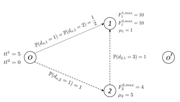
Figure 1: Labels satisfying dominance rule 5.1 and violating rule 5.2

Example 5.3

Figure 1 visualizes the pricing network for a disaggregated profile $(q,s)\in\mathcal{Q}^{D}$ and two labels $L^{1}$ (solid line) and $L^{2}$ (dotted line). We assume $\mathcal{K}=\{1\}$, $s_{q,1}=1$ and $\delta_{1,\tau}=-1$ for all $\tau\in[0,10]$. Furthermore, we simplify our considerations by neglecting time window restrictions and setting $w_{1}=w_{2}=1$. Moreover, we define $p_{2,q}=3$ and $p_{1,q}=3$. The reduced costs for labels $L^{1}$ and $L^{2}$ are then equal to $T_{1}^{1,cost}=13.5$ and $T_{2}^{2,cost}=18$. Therefore, it is clear to see that $L^{1}$ dominates $L^{2}$ in the sense of Definition 5.1. However, if we offset the reduced cost of each label by the workforce penalties, we obtain

$$T_{1}^{2,cost}+\underset{\tau=0}{\overset{10}{\sum}}\delta_{1,\tau}\beta_{k,\tau}^{s,2}(\omega_{max})=18-11=7<7.5=13.5-6=T_{1}^{1,cost}+\underset{\tau=5}{\overset{10}{\sum}}\delta_{1,\tau}\beta_{k,\tau}^{s,1}(\omega_{max})$$

Hence, $L^{1}$ does not dominate $L^{2}$ in $\mathcal{G}^{q,s}$, i.e., in the sense of Definition 5.2. The dominance rule presented here tends to be more strict, leading to around 25% less dominated labels.

As the only difference between the pricing graphs $\mathcal{G}^{q,\tilde{s}}$ and $\mathcal{G}^{q,s}$ for $q\in\mathcal{Q}$ and $s,\tilde{s}\in\mathcal{S}_{q}$ lies in the workforce penalty for the dynamic arc weights, we can transfer any feasible label $L=\left(tl^{L},v,P,T_{v}^{cost},(T_{v,i}^{perf})_{i\in\mathcal{\hat{I}}_{q}},F_{v}^{L},F_{v}^{L,max},tl^{L}\right)$ in $\mathcal{G}^{q,s}$ to a different pricing network $\mathcal{G}^{q,\tilde{s}}$ and obtain a new feasible label $\tilde{L}$ in $\mathcal{G}^{q,\tilde{s}}$ with

$$\tilde{L}=\left(tl^{L},v,P,\tilde{T}_{v}^{cost},(T_{v,i}^{perf})_{i\in\mathcal{\hat{I}}_{q}},F_{v}^{L},F_{v}^{L,max},tl^{L}\right)$$

that is, all properties besides the reduced cost $T_{v}^{cost}$ of $L$ remain the same. As the dominance rule on $\mathcal{G}^{q,s}$ merely considers reduced costs after offsetting them by the workforce penalty, it is clear to see that if a label $L^{1}$ dominates another label $L^{2}$ in $\mathcal{G}^{q,s}$ if and only if it dominates $L^{2}$ in $\mathcal{G}^{q,\tilde{s}}$ for all $\tilde{s}\in\mathcal{S}_{q}$. For a formal proof of these relations, see Appendix 11.
Therefore, for a profile $q\in\mathcal{Q}$, the column with minimum reduced cost for the set $\left((q,s)\right)_{s\in\mathcal{S}_{q}}$ of disaggregated profiles can be calculated as follows: we select an arbitrary skill composition $\tilde{s}\in\mathcal{S}_{q}$ and solve the ESPPRC on $\mathcal{G}^{q,\tilde{s}}$. After no further labels can be created, the following optimization problem on the set $\mathcal{L}$ of non-dominated labels present at the sink $o^{\prime}$ is solved to obtain a route with profile $q$, an optimal skill composition $s^{*}$ and minimal reduced cost:

$$\min\left\{T^{L,cost}_{o^{\prime}}+\underset{\tau=tl^{L}}{\overset{tr^{L}}{\sum}}\delta_{k,\tau}\beta_{k,\tau}^{\tilde{s}}-\underset{\tau=tl^{L}}{\overset{tr^{L}}{\sum}}\delta_{k,\tau}\beta_{k,\tau}^{s}:\ s\in\mathcal{S}_{q},\ L\in\mathcal{L}\right\}$$

Because the number of labels at the sink and the number of possible skill compositions is usually small, this problem can be solved by explicit enumeration. In total, the runtime savings by solving one pricing network (instead of multiple) for each profile exceeds the additional runtime caused by a weaker dominance rule by magnitudes.

5.4 Acceleration Strategies

As the pricing step is by far the most runtime-intensive component in the proposed solution approach, we employ several strategies that allow us to generate columns with negative reduced costs more quickly. In the following, we describe these techniques in detail.

Graph Size Reduction

We use two heuristics that initially reduce the graph size and set of initial labels and gradually increase them when necessary. The first heuristic consists of separating the set of possible depot leave times (19) into bins {1,…,B} of equal size and sorting these bins in an ascending order with respect to the minimum reduced cost of all labels inside the bin. We then solve the ESPPRC considering only the initial labels in bin $1$. If no column with negative reduced costs has been found, we continue with the next bin until we either find a negative column or solve the final bin $B$. In our algorithm, we set the value $B$ such that each bin $\{1,\dots,B-1\}$ has a size of $5$.
The second heuristic is similar to the one proposed by Desaulniers, Lessard, and Hadjar (2008). For each task node $i$, we sort the set of outgoing arcs $(i,j)\in\mathcal{A}^{q}$ with $j\in\mathcal{\hat{I}}_{q}$ based on their task duals $\mu_{j}$. Initially, we only allow extensions along $(i,j)$ if $\mu_{j}$ is among the $\Delta$ largest dual values of task nodes adjacent to $i$. If we do not find a negative column, we solve the pricing problem while allowing extensions along all arcs.
In our experiments, we set $\Delta=4$ as this returned the best results. Furthermore, we first iterate through all initial label bins and then switch to allowing extensions along all arcs only if no negative column has been found in any of the bins.

Decremental State Space Relaxation

Decremental state space relaxation has first been proposed by Christofides, Mingozzi, and Toth (1981) and relies on reducing the dimension of the state space, i.e., the number of resources tracked. Hence, the ESPPRC is solved using labels with fewer resources, allowing for generally stronger dominance relations. We relax our state space by replacing the task resources $\left(T_{v,i}^{perf}\right)_{i\in\mathcal{\hat{I}}}$ of a label $L$ by the length $l_{P}$ of the path $P$ corresponding to $L$. Thus, we allow extensions to a task node $i$ even if $T_{v,i}^{perf}=0$. Dominance rules 5.1 and 5.2 are then adjusted by replacing inequality (16) or (21) with $l_{1}\leq l_{2}$. Whenever a negative column visiting a task node $i$ multiple times is returned, we re-insert the corresponding task resource $T_{v,i}^{perf}$ into the dominance rule. This step is repeated until the optimal column does not contain any cycles or has non-negative reduced costs.

5.5 Branching Strategies

We use three different branching rules to cut off fractional solutions of the ARMP or DRMP. In the following, we summarize these strategies and their technicalities.

Branching on Task Finish Times

Gélinas et al. (1995) were among the first ones to branch on resource windows, more specifically, time windows. While this strategy is not novel, the process of selecting a task and a time instant to branch on has a significant impact on the branching rule’s efficiency. Let $(\bar{\lambda}^{r})_{r\in\mathcal{R}}$ be an optimal solution to the ARMP and let $\mathcal{R}_{F}\subseteq\mathcal{R}$ be the set of columns for which $\bar{\lambda}^{r}$ is fractional. For each task $i\in\mathcal{I}$, we define

$$\mathcal{B}^{F}(i)\coloneqq\left\{F_{i}^{r,q}(\omega_{max}):\ (r,q)\in\mathcal{R}_{F}:\ i\in r\right\},$$

$$\mathcal{B}^{F}_{U}(i)\coloneqq\left\{F_{i}^{r,q}(\omega_{max}):\ (r,q)\in\mathcal{R}_{F}:\ i\in r,\ F_{i}^{r,q}(\omega_{max})\ \text{unique}\right\}$$

as the set of all (unique) worst-case finish times of task $i$ within team routes with fractional values, respectively. We then select all tasks for which the cardinality of the latter set is maximal and denote it by $\mathcal{I}^{F}$, i.e.,

$$\mathcal{I}^{F}=\left\{i\in\mathcal{I}:\left|\mathcal{B}^{F}_{U}(i)\right|=\max\left\{\ \left|\mathcal{B}^{F}_{U}(j)\right|:\ j\in\mathcal{I}\right\}\right\}.$$

We then select the task $i^{*}$ for which the standard deviation of the worst-case finish times of task $i^{*}$ in all routes in $\mathcal{B}^{F}(i)$ is maximal, that is

$$i^{*}=\argmax\left\{\sigma\left(\left\{F_{i}^{r,q}(\omega_{max}):\ (r,q)\in\mathcal{B}^{F}(i)\right\}\right):\ i\in\mathcal{I}^{F}\right\}$$

where $\sigma(\cdot)$ is the standard deviation of a finite set. We then branch on task $i^{*}$ and time instant $\tau^{*}=\left\lfloor M(\mathcal{B}^{F}(i^{*}))\right\rfloor$, where $M(\cdot)$ is the median of a finite set. We then create two child nodes and impose constraints

$$F_{i^{*}}^{r,q}(\omega_{max})\leq\tau^{*}\quad\forall(r,q)\in\mathcal{R}:\ i^{*}\in r\quad\text{or}\quad F_{i^{*}}^{r,q}(\omega_{max})>\tau^{*}\quad\forall(r,q)\in\mathcal{R}:\ i^{*}\in r,$$

respectively. Furthermore, we remove all tours that violate the constraints from the child nodes. In the pricing steps, we forbid extensions that would violate these task finish time constraints. If

$$\max\left\{\sigma\left(\left\{F_{i}^{r,q}(\omega_{max}):\ (r,q)\in\mathcal{B}^{F}(i)\right\}\right):\ i\in\mathcal{I}^{F}\right\}=0$$

holds, we know by construction that in the current solution, $\left|\mathcal{B}^{F}_{U}(i)\right|=1$ holds for all $i\in\mathcal{I}$. Therefore, independent of the selection of $i^{*}$ and $\tau^{*}$, the above branching rule does not produce a nontrivial branch. If this is the case, a different branching strategy must be used. We note that the above branching strategy does not change the master problem’s structure.

Branching on Number of Tours at a Given Time

Desrochers, Desrosiers, and Solomon (1992) introduced branching on tour counts, which has proven to be efficient for vehicle routing problems. Let $\tau^{*}$ be the time instant for which $l_{\tau^{*}}=\underset{r\in\mathcal{R}}{\sum}g_{\tau^{*}}^{r}\lambda^{r}_{q}$ is closest to 0.5, where $g_{\tau}^{r}=1$ if $tl^{r}\leq g_{\tau}^{r}\leq tr^{r}$ and $g_{\tau}^{r}=0$ else. We then branch on the current solution by imposing

$$\underset{r\in\mathcal{R}}{\sum}g_{\tau^{*}}^{r}\lambda^{r}_{q}\leq\lfloor l_{\tau^{*}}\rfloor\quad\text{or}\quad\underset{r\in\mathcal{R}}{\sum}g_{\tau^{*}}^{r}\lambda^{r}_{q}\geq\lceil l_{\tau^{*}}\rceil.$$ (25)

The pricing problem has to be adjusted in the sense that dynamic arc weights have to consider the dual cost of the additional inequalities. If a label $L$ is extended along an arc $(v,v^{\prime})$ and $F_{v^{\prime}}^{L}(\omega_{max})<\tau^{*}\leq F_{v^{\prime}}^{L}(\omega_{max})$ holds, the cost of arc $(v,v^{\prime})$ must be adjusted by the dual cost of (25). Similar to branching on task finish times, this branching strategy can potentially produce a trivial branch, making a fallback branching option necessary.

Branching on Variables

If both previously described branching rules fail to produce a nontrivial branching decision, we select the most fractional variable $\lambda^{r^{*}}_{q^{*}}$ and set it to $0$ or $1$ in the child nodes. When a team route $(r^{*},q^{*})$ is forced, i.e., $\lambda^{r^{*}}_{q^{*}}=1$ is enforced, we remove all tasks which are visited by $r^{*}$ from the pricing networks, discard all team routes that share tasks with $r^{*}$ and adequately reduce the total available workforce $N_{k}$ and $N_{k}^{D}$ for all $k\in\mathcal{K}$. When a team route $(r^{*},q^{*})$ is forbidden, we introduce an additional resource to the pricing problem that tracks how many arcs a label has used that correspond to segments of $r^{*}$. If this resource is fully consumed, we discard the label as it equals a forbidden tour. For the DRMP, we do not discard said labels but skip the skill composition $s$ that is used to execute the forbidden route. Furthermore, if a label is equal to a subpath of a forbidden tour, it can not dominate any other label as this might lead to cutting off optimal labels.

5.6 Cutting Planes

Whenever a fractional optimal solution is found at a node in the branching tree, we model the problem of finding a most violated rank-1 Chvátal-Gomory cut (CGC) as a mixed-integer problem and solve it exactly using a generic solver with a very short time limit. This approach was first proposed by Fischetti and Lodi (2007) and applied to a vehicle routing problem with time windows by Petersen, Pisinger, and Spoorendonk (2008). In the following, we base our considerations on the ARMP formulation. Let $(u_{i})_{i\in\mathcal{I}}\in[0,1)$ and $(u_{k,t})_{k\in\mathcal{K},t\in\mathcal{T}}$ be the coefficients of the most violated cut. We then add the constraint

$$\underset{(r,q)\in\mathcal{R}}{\sum}\left\lfloor\underset{i\in\mathcal{I}^{r}}{\sum}u_{i}+\underset{k\in\mathcal{K}}{\sum}\ \underset{\tau=tl^{r}}{\overset{tr^{r}}{\sum}}b_{k,\tau}^{q}(\omega_{max})u_{k,t}\right\rfloor\lambda^{r}_{q}\leq\left\lfloor\underset{i\in\mathcal{I}^{r}}{\sum}u_{i}+\underset{k\in\mathcal{K}}{\sum}N_{k}\cdot\left(\underset{\tau\in\mathcal{T}}{\sum}u_{k,t}\right)\right\rfloor$$

to the master problem and re-solve the current node.
Let $\mathcal{G}$ be the set of indices of CGCs and $\mathcal{C}^{\mathcal{G}}\coloneqq\{\left((u_{i}^{g})_{i\in\mathcal{I}},(u_{k,t}^{g})_{k\in\mathcal{K},t\in\mathcal{T}}\right):\ g\in\mathcal{G}\}$ be the cut coefficients for all CGCs present at the current node. During the pricing step, we introduce an additional resource $T_{v,g}$ for each CGC $g\in\mathcal{G}$. When extending a label $L\coloneqq\left(tl^{L},v,P,T_{v}^{cost},(T_{v,i}^{perf})_{i\in\mathcal{\hat{I}}_{q}},(T_{v,g})_{g\in\mathcal{G}},\mathcal{F}_{F_{v}^{L}},F_{v}^{L,max}\right)$ along an arc $(v,v^{\prime})$, we update the resources $(T_{v,g})_{g\in\mathcal{G}}$ and $T_{v^{\prime}}^{cost}$ using the following resource extension function:

$$T_{v^{\prime}}^{cost} =T_{v}^{cost}+\left\lfloor T_{v,g}+u_{v^{\prime}}^{g}+\underset{k\in\mathcal{K}}{\sum}\ \underset{\tau=F_{v}^{L,max}}{\overset{F_{v^{\prime}}^{L^{\prime},max}}{\sum}}b_{k,\tau}^{q}(\omega_{max})u_{k,t}^{g}\right\rfloor\cdot\psi_{g}$$

$$T_{v^{\prime},g} =T_{v,g}+u_{v^{\prime}}^{g}+\underset{k\in\mathcal{K}}{\sum}\ \underset{\tau=F_{v}^{L,max}}{\overset{F_{v^{\prime}}^{L^{\prime},max}}{\sum}}b_{k,\tau}^{q}(\omega_{max})u_{k,t}^{g}-\left\lfloor T_{v,g}+u_{v^{\prime}}^{g}+\underset{k\in\mathcal{K}}{\sum}\ \underset{\tau=F_{v}^{L,max}}{\overset{F_{v^{\prime}}^{L^{\prime},max}}{\sum}}b_{k,\tau}^{q}(\omega_{max})u_{k,t}^{g}\right\rfloor$$

where $\psi_{g}\geq 0$ is the dual variable associated with CGC $g\in\mathcal{G}$. Dominance rule 5.1 is then slightly adjusted and extended:

Definition 5.4 (Dominance Rule)

Let

$$L^{k}\coloneqq\left(tl^{k},v,P^{k},T_{v}^{k,cost},(T_{v,i}^{k,perf})_{i\in\mathcal{\hat{I}}_{q}},(T_{v,g}^{k})_{g\in\mathcal{G}},F_{v}^{k},F_{v}^{k,max}\right)$$

be labels for $k=1,2$. Let $\mathcal{G}$ be the set of indices of CGCs and $\mathcal{G}^{>}\coloneqq\left\{g\in\mathcal{G}:\ T_{v,g}^{1}>T_{v,g}^{2}\right\}$. We say that $L^{1}$ dominates $L^{2}$ if constraints (16)–(18) and

$$T_{v}^{1,cost}+\underset{g\in\mathcal{G}^{>}}{\sum}\psi_{g} \leq T_{v}^{2,cost}$$ (26)

$$T_{v,g}^{1} \leq T_{v,g}^{2}\quad\forall g\in\mathcal{G}\setminus\mathcal{G}^{>}$$ (27)

hold.

Inequalities (26) and (27) ensure that for any feasible extension $(v,v^{\prime})$ of $L^{2}$, the reduced costs still remain dominated by $L^{1}$. For a proof of correctness of this approach, we refer to Section 4 of Petersen, Pisinger, and Spoorendonk (2008).
Identifying violated CGCs can be quite costly if repeated frequently. Furthermore, each CGC slightly weakens the dominance rule due to the additional constraints (27), and calculating the coefficients $T_{v,g}$ requires additional computational effort. Hence, limiting the maximum amount of CGC present at any node in the search tree can be beneficial. Finally, we note that the above CGCs remain feasible when the master problem formulation is switched to the DRMP.

5.7 An early Termination Heuristic

Because several exterior factors, such as unexpected aircraft delays, can create the need for re-optimization, limiting the maximum runtime of the Branch-Price-Cut-and-Switch scheme is often necessary. Let $\bar{\mathcal{R}}$ and $\bar{\mathcal{R}^{D}}$ be the sets of columns found during the branch-and-price procedure for the ARMP and DRMP, respectively. We then define the set $\mathcal{R}^{D,H}$ as

$$\mathcal{R}^{D,H}\coloneqq\left\{(r,q,\tilde{s}):(r,q)\in\bar{\mathcal{R}},\tilde{s}\in\mathcal{S}_{q}\right\}\ \cup\ \left\{(r,q,\tilde{s}):\exists s\in\mathcal{S}_{q}:\ (r,q,s)\in\bar{\mathcal{R}^{D}},\tilde{s}\in\mathcal{S}_{q}\right\}$$

Whenever the time limit is reached, we solve the DMP (10)–(13), including integrality constraints, on the column set $\mathcal{R}^{D,H}$. If a feasible solution has been found within a prespecified time limit, we return the solution as the best integer solution found.

6 Experimental Study

In the following, we analyze the impact of cutting planes, switching between the DRMP and ARMP as master problem formulations and different branching strategies on solution quality and convergence speed. Furthermore, we compare stochastic and deterministic solutions and evaluate the impact of stochasticity on optimal strategies.
Section 6.1 elaborates on the generation of test instances. Section 6.2 summarizes the algorithm’s performance for different configurations of the aforementioned components. In Section 6.3, stochastic and deterministic optimal policies are compared with respect to their practical feasibility. The algorithm is implemented using Python 3.11 and Gurobi 10.0.2. Furthermore, all computational studies were performed on a single machine equipped with an Intel® Xeon® W-1390p 11th gen 8-core 3.5GHz processor, 32GB of RAM and running Windows 10. All instances and corresponding solutions can be found under https://github.com/andreashagntum/StochasticTeamFormationRoutingAirport.

6.1 Instance Set

We use the instance generator developed by Dall’Olio and Kolisch (2023) to construct a set of test instances of different complexity. A predefined number of flights and their characteristics, such as time windows and parking positions, are generated based on realistic assumptions from Munich Airport. In the following, we briefly elaborate on parameters that have been varied throughout the generation.
In order to generate instances of different sizes, we vary the length of the planning horizon between 60, 90, and 120 minutes and generate 10, 20, or 30 flights per hour. The underlying time grid consists of equidistant time steps with a length of 2 minutes. Each type of airplane served at Munich Airport can be loaded using one of up to 3 different team formations, called slow, intermediate, and fast mode. Faster modes use up more workers but require less time to (un)load an aircraft. Not every plane can be loaded with all 3 modes, especially smaller planes typically only support slow or fast modes. We note that the same properties hold for unloading tasks. We generate multiple instance sets by restricting the available team formations to only the intermediate mode, to the slow and the fast mode, or to all three modes, respectively. Furthermore, the available workforce ranges between 10% and 90% of the workers required when all tasks are started at the earliest possible time with the fastest possible mode. In the following, this factor is referred to as worker strength. Lastly, the minimum service level is set to $\alpha=0.9$ and the extended latest finish time is set to $LF_{i}^{e}=LF_{i}+5$, i.e., 5 time steps after the latest finish time. We generated five random flight schedules for each combination of the aforementioned parameters, leading to a total of $3\cdot 3\cdot 3\cdot 9\cdot 5=1,215$ instances. We note that the largest test instances in this set, namely instances with a 2-hour planning horizon, 30 flights per hour, and three available modes, replicate the most complex instances one might encounter at Munich Airport.
All further properties, such as flight schedules and task execution times, are calculated as described by Dall’Olio and Kolisch (2023). For a precise description of the process, the interested reader is referred to Section 6.1 and Appendices E and F of their paper.
We approximate the distribution of travel times between locations using empirical data. For this purpose, we collected real-world data on travel times of various ground operating vehicles, such as passenger buses and baggage handling vehicles, at Terminal 2 of Munich Airport for seven consecutive days in September 2022. These values, if needed, are adjusted to baggage handling vehicles by scaling them proportionally by their respective average speeds. The data is then used to derive empirical probability density functions for each pair of parking positions.

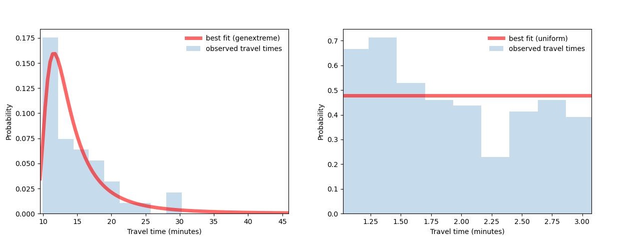
Figure 2: Exemplary empirical and approximate distributions of travel times

Based on our empirical data, we conduct Kolmogorov-Smirnov tests to better understand the structure of travel time distributions. We observe that said distributions are best approximated with either a positively-skewed, generalized extreme value distribution with a shape parameter between $-0.6$ and $1.1$ (left graph of Figure 2) or a uniform distribution (right graph of Figure 2). Generally, the larger the distance between two parking positions is, the more the travel time distribution resembles the extreme value distribution and the larger the shape parameter is.

6.2 Influence of the Algorithm’s Features

From a methodological point of view, our solution approach differs from the ones typically used for variants of vehicle routing or team formation problems in three ways: dynamically switching between two master problem formulations, branching on task finish times and an exact separation of rank-1 CGCs. In the following, these are called the algorithm’s features. In this section, we compare a total of five solver configurations: we first enable and then disable all three features, resulting in what are called ‘full’ and ‘basic’ configurations, respectively. Furthermore, we disable exactly one feature to obtain three additional variants of our solution method called ‘no DRMP’, ‘no CGCs’ and ‘no branching on task finish times’ (also abbreviated as ‘no branching’). For instance, the configuration ‘no DRMP’ uses branching on task finish times and adds up to 12 CGCs at the root node, but does not dynamically switch to the DRMP master problem formulation. We note that we do not include solver configurations with exactly two features enabled in our analysis, as the results do not fundamentally differ from the ones presented in the following.

Feature Design

We configure the aforementioned features as follows. When branching, we first try to branch on task finish times by using the procedure described in Section 5.5. If that is not possible, we look for branches on vehicle counts and, if this also fails, we use the fallback option of branching on variables. Furthermore, whenever a disaggregated-infeasible solution is found, we switch to solving the DRMP formulation at the current node and its sibling node. Additionally, child nodes of DRMP nodes inherit their master problem’s type, i.e., they are also solved using the DRMP formulation. Finally, we only search for violated CGCs at the root node and add up to 12 cuts. The MIP required to identify such cuts, as described by Fischetti and Lodi (2007) is solved using Gurobi with a time limit of 0.3 seconds. For each instance, a hard time limit of 180 seconds is imposed. If no optimal solution has been found, an upper bound is obtained by the procedure described in Section 5.7. We note that preliminary studies have shown that adding up to 12 cuts, on average, provides an optimal trade-off between lower bound improvements and an increase in computational complexity.

Instance Set and Instance Classes

Each of the aforementioned 5 configurations is used to solve the instance set generated as described in Section 6.1, amounting to a total of 1,215 instances per configuration. In total, 615 instances are infeasible. We omit said instances and compare the ascribed feature configurations on the remaining 600 instances.
In order to distinguish between easy and hard instances, we split the set of test instances into three categories. In preliminary studies, the worker strength has proven to have a significant impact on an instance’s complexity. Therefore, we consider instances with a worker strength between 0.3 and 0.5 as ‘hard’, while instances with a strength of 0.6 or 0.7 are seen as ‘medium’ and 0.8 or 0.9 as ‘easy’. In fact, almost all instances in the latter category were solved within a few seconds, whereas instances in the hard category are frequently not solved to optimality within the set time limit. We note that all instances with a worker strength of 0.2 or less are infeasible, while only 2 instances with a worker strength of 0.3 are feasible.
Unless otherwise stated, all tables in this section, contain average values. The number of instances on which the following analyses are based can be seen in Appendix LABEL:appendix_instance_set_sizes.

Comparison of Full and Basic Configuration

Table 2: Comparison of basic and full solver configuration

Instance Class	Config	% Opt	Gap %	UB	LB	Runtime
Easy	Full	100.00%	0.00%	2.74	2.74	1.74s
	Basic	82.38%	6.81%	2.74	2.02	34.55s
Medium	Full	90.61%	0.49%	15.41	15.29	28.90s
	Basic	61.50%	6.57%	15.43	14.30	78.17s
Hard	Full	62.70%	2.75%	64.26	61.64	87.75s
	Basic	56.35%	4.07%	64.29	60.88	96.51s
All	Full	88.83%	0.75%	20.16	19.56	29.44s
	Basic	69.50%	6.15%	20.17	18.74	63.05s

Table 2 compares the results obtained using the full configuration with the basic configuration. Column “% Opt” contains the percentage of instances that have been solved to optimality. It can be seen that the full configuration solves 19% more instances to optimality than the basic configuration. Furthermore, it returns significantly better average optimality gaps for all instance classes, where this effect decreases with increasing worker strength. While the full configuration returns substantially better lower bounds for all instance classes, the upper bounds also increased slightly for harder instances. Moreover, runtimes for small and medium instances reduce drastically, while larger instances are solved around 8 seconds faster on average.

Solution Quality Robustness

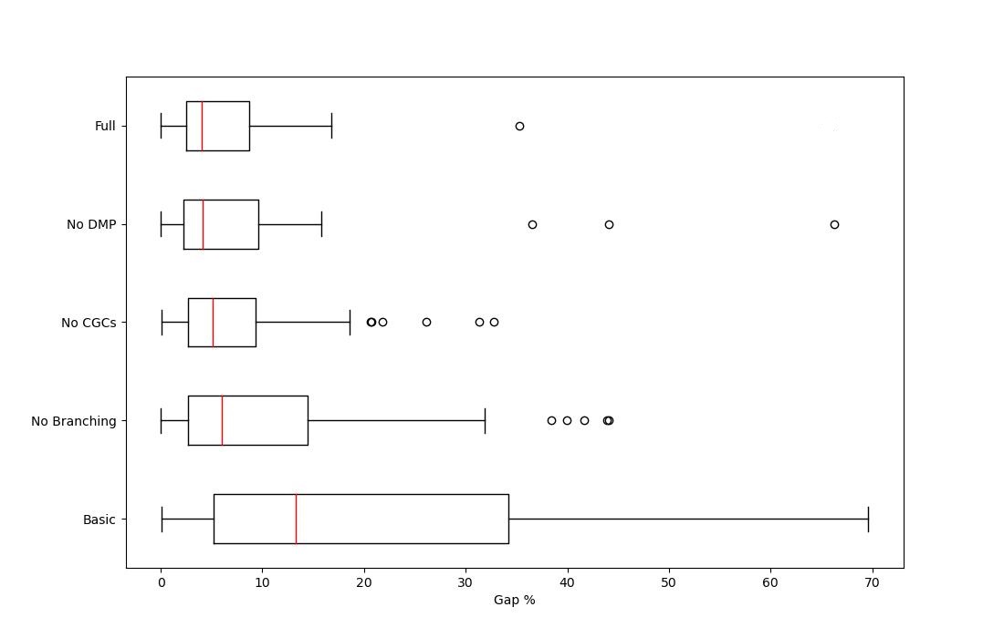
Figure 3: Box plot of optimality gap percentage for all solver configurations

Figure 3 visualizes the frequencies of non-zero optimality gap percentages for all five considered solver configurations in a box plot. The red line is the median, while the boxes are limited by the 25%- and 75%-quantiles. The lower and upper whiskers are calculated as $q_{0.25}-1.5\cdot IQR$ and $q_{0.75}+1.5\cdot IQR$, respectively, where $IQR=q_{0.75}-q_{0.25}$ is the interquartile range. Clearly, the basic configuration has a high median optimality gap, as well as a comparable large set of outliers, sometimes even terminating with a gap of close to 70%. These metrics generally improve when enabling two of the three algorithm’s features, while the best results can be observed when using the full solver configuration. Additionally, larger gap percentages occur rather frequently when using the basic configuration, as all instances lie within their respective whiskers. Hence, the full solver configuration returns the best and most stable results from all compared strategies.

Full vs. No Branching

Table 3: Comparison of full and no branching on task finish times configuration

Instance Class	Config	% Opt	Gap %	UB	LB	Ropt	Nopt	Nexp	Rnode	Rpr
Easy	Full	100.00%	0.00%	2.74	2.74	1.22s	1.08	1.32	1.32	0.039s
	No Branching	99.23%	0.12%	2.74	2.72	1.23s	1.20	3.37	0.92	0.041s
Medium	Full	90.61%	0.49%	15.41	15.29	4.13s	5.84	34.42	0.84	0.090s
	No Branching	75.59%	2.64%	15.43	14.82	7.14s	11.17	54.11	0.94	0.197s
Hard	Full	62.70%	2.75%	64.26	61.64	17.59s	32.52	87.55	1.00	0.209s
	No Branching	58.73%	4.19%	66.64	61.00	19.02s	26.31	56.67	1.61	0.327s
All	Full	88.83%	0.75%	20.16	19.56	4.38s	6.88	31.18	0.94	0.093s
	No Branching	82.33%	1.87%	20.66	19.25	5.53s	7.80	32.58	1.18	0.157s

Table 3 compares the results obtained by the full solver configuration with the configuration ‘no branching’, i.e., branching on task finish times is disabled. Columns “Ropt” and “Nopt” describe the runtime and the number of explored nodes until optimality has been proven. We note that, unlike all other values in the above table, the baseline for these two metrics is not the entire instance set of a fixed instance class, but instead the set of instances that has been solved to optimality by both solver configurations. Column “Nexp” describes the number of explored nodes, while “Rnode” and “Rpr” contain the runtime per explored node and the runtime per pricing iteration, respectively. The average solution quality improves when the branching strategy is enabled, as 6.50% additional instances are solved to optimality, and the average gap is reduced by around 1%. Furthermore, solving a single node requires, on average, 20% less time, where this improvement increases for harder instances. This can be explained by significant time savings in the pricing step, where the runtime decreases from 0.327 seconds per iteration to 0.209 seconds.
For easy and medium instances, the full solver configuration requires less time to prove optimality and explores around 10% to 50% fewer nodes to do so, respectively. For the set of hard test instances, using branching on task finish times improves the solution quality noticeably, while optimality gaps are reduced by 1.44%. However, around 20% more nodes are required to prove optimality. This indicates that for larger instances, branching on task finish times is able to provide very good lower bounds, but does not excel at proving optimality. In summary, task finish times appear to be an efficient basis for branching decisions, as they significantly simplify the pricing step. For more complex instances, further studies on a potential tail-off effect on the quality of lower bounds and possible ways to mitigate this issue are needed.

Full vs. no DRMP

Table 4: Comparison of full and no DRMP configuration

Instance Class	Config	% Opt	Gap %	UB	LB	Ropt	Nopt	ARMPn	DRMPn	NoAinf
Easy	Full	100.00%	0.00%	2.74	2.74	1.26s	1.16	8.00	7.70	1.33
	No DMP	99.62%	0.01%	2.74	2.74	1.27s	1.17	5.70	0.00	1.67
Medium	Full	90.61%	0.49%	15.41	15.29	8.03s	15.21	19.60	16.90	1.40
	No DMP	88.26%	0.80%	15.41	15.27	8.46s	16.27	67.70	0.00	22.73
Hard	Full	62.70%	2.75%	64.26	61.64	17.18s	21.08	155.00	40.70	1.58
	No DMP	56.35%	3.26%	66.5	61.6	19.58s	28.26	186.70	0.00	12.17
All	Full	88.83%	0.75%	20.16	19.56	5.72s	8.71	72.60	25.5	1.47
	No DMP	86.50%	0.97%	20.63	19.55	6.19s	10.02	109.10	0.00	16.40

Table 4 combines the results obtained by the full solver configuration with the ‘no DRMP’ configuration, i.e., whenever a disaggregated-infeasible solution is identified, the solution is forbidden explicitly using a constraint of type $\underset{r\in\mathcal{\bar{R}}}{\sum}\lambda^{r}\leq|\mathcal{\bar{R}}|-1,$ where $\mathcal{\bar{R}}$ is the set of columns selected by an optimal, disaggregated-infeasible solution. For medium and large instances, 2.5% to 6% more instances can be solved to optimality and average gaps decrease by around 0.5% when using the DRMP formulation. Columns “ARMPn” and “DRMPn” contain the number of nodes solved using the ARMP and DRMP formulation, respectively. Additionally, column “NoAinf” contains the average number of disaggregated-infeasible solutions. For these three columns, the baseline set of instances are all instances for which at least one of the two configurations has found at least one disaggregated-infeasible solution. The number of such solutions found is large for medium and hard instances, while less than 2 disaggregated-infeasible solutions are found when using the DRMP formulation. This, jointly with the small share of nodes solved using the DRMP, further solidifies our assumption that such solutions only occur on very few branches of the branching tree, underlining the reasonability of our approach of only switching to the DRMP within branches that returned such undesired solutions.

Full vs. no CGCs

Table 5: Comparison of full and no Gomory cut configuration

Instance Class	Config	% Opt	Gap %	UB	LB	Rnode	RneR	% Root solved	RootLB
Easy	Full	100.00%	0.00%	2.74	2.74	1.32s	1.92s	95.40%	2.71
	No CGCs	97.70%	0.34%	2.74	2.71	0.41s	0.42s	47.89%	1.86
Medium	Full	90.61%	0.49%	15.41	15.29	0.84s	0.72s	53.05%	14.46
	No CGCs	86.85%	0.92%	15.41	15.23	0.42s	0.41s	14.08%	13.29
Hard	Full	62.70%	2.75%	64.26	61.64	1.00s	0.80s	30.16%	59.43
	No CGCs	61.11%	2.42%	64.17	61.86	0.64s	0.60s	5.56%	57.56
All	Full	88.83%	0.75%	20.16	19.56	0.94s	0.77s	66.67%	18.79
	No CGCs	86.17%	0.98%	20.14	19.58	0.52s	0.50s	27.00%	17.61

Table 5 analyzes the results obtained by the full configuration and compares it to the ‘no CGCs’ configuration, i.e., no CGCs are added. Column “rootLB” contains the lower bound obtained after solving the root node, while column “RneR” depicts the algorithm’s runtime per node, excluding the root node. On average over all test instances, the usage of Gomory cuts improves the final lower bounds, allowing us to solve 2.5% more instances to optimality and closing the optimality gap by an additional 0.2%. Furthermore, the percentage of instances solved at the root node more than doubles from 27% to 66.67%, while it even increases six-fold for hard instances. Moreover, the lower bound at the root node improves by around 7%. Additionally, column “RnerR” shows that CGCs significantly increase the runtime per non-root node, rising by 54% from 0.50 seconds to 0.77 seconds on average. Altogether, Gomory cuts aid to provide excellent bounds early on during the solving procedure. However, the increase in computational complexity, especially during the pricing step, implies a trade-off between bound quality and computational complexity. Especially for larger instances, carefully separating and electing CGCs plays a crucial role in the approach’s efficiency.
To conclude this section, we showed that our developed solution strategy is able to significantly improve the ‘basic’ configuration first described by Dall’Olio and Kolisch (2023), both with respect to optimality guarantees and bound quality. While the impact of every single configuration’s component seems to be rather small, combining our three core features and using them simultaneously greatly benefits the resulting algorithm’s performance.

6.3 Stochastic and Deterministic Solutions

In the following, we compare the quality of stochastic solutions with that of deterministic ones. For that purpose, all 1,215 test instances are solved using our stochastic approach and three deterministic approaches assuming best-case, median, or worst-case travel times. We note that we can adjust the AMP to use deterministic travel times $\tau_{i,j}$ for tasks $i$ and $j$ by assuming $P(t_{i,j}=\tau)=1$ when constructing the respective master problem. We thus obtained a total of four solutions for each instance, one for each type of deterministic travel time and one for stochastic travel times. We then sample 1,000 scenarios for each instance by randomly generating travel times for all pairs of parking positions according to the respective empirical distributions. For each instance and each scenario, we analyze the finish times of all tasks for all four solutions. By aggregating these results for each instance and solution over all 1,000 scenarios, we obtain an empirical service level and objective function value (10), which allows us to further assess the performance of deterministic and stochastic solutions. Furthermore, we use the deterministic framework, i.e., constraints (3) and (4) need to be satisfied. For deterministic travel times, this is equivalent to using hard time windows $[ES_{i},LF_{i}]$ for each task $i$ and disallowing delays. In the following, we refer to the solution of an instance when using stochastic travel times as the stochastic solution of an instance. For best-, median, and worst-case travel times, we analogously refer to best-, median, and worst-case travel time solutions, respectively.

Table 6: Frequencies of stochastic (in)feasibility

		Deterministic	Stochastic
Complexity	Travel Times	#Feas.	#alpha-feas.	#LFe-feas.	#Stoch.-feas.
Easy	Best	266	16	38	13
	Median	265	151	250	150
	Worst	261	261	261	261
	Stochastic	261	261	261	261
Medium	Best	243	15	34	12
	Median	228	123	196	117
	Worst	207	207	207	207
	Stochastic	213	213	213	213
Hard	Best	219	0	21	0
	Median	156	43	105	37
	Worst	110	110	110	110
	Stochastic	126	126	126	126
All	Best	728	31	93	25
	Median	649	317	551	304
	Worst	578	578	578	578
	Stochastic	600	600	600	600

Table 6 summarizes the feasibility of instances and solutions under various travel time assumptions. For each type of travel time, column “#Feas.” contains the number of instances whose master problem (10)–(13) is feasible, assuming the respective travel times. Furthermore, column “#Alpha-feas.” denotes the number of instances whose solutions satisfy the desired service level $\alpha$ for each task. This requirement is equivalent to satisfying constraint (3). Column “#LFe-feas.” serves a similar purpose and contains the number of instances whose solutions guarantee no delays beyond extended latest finish times. This corresponds to satisfying equality (4). Finally, column “#Stoch.-feas.” contains the number of instances whose solutions were feasible with respect to the prescribed requirements regarding both service levels and maximum delays. This is equivalent to fulfilling constraints (3) and (4) simultaneously. It is clear to see that a decrease in the available workforce increases the frequency with which the prescribed service level is not satisfied or large delays can not be ruled out. Furthermore, only 31 out of 728 best-case travel time solutions satisfy the desired service level for all tasks, while only 25 solutions are feasible with respect to both service level and maximum delay constraints. When median travel times are assumed, around 49% of all solutions guarantee the desired service level, while only 304 out of 649, i.e., around 47% of solutions also fulfill the maximum delay requirement (4). Thus, if deterministic travel times are assumed, it is likely that either tasks are delayed with a probability of more than $1-\alpha$ or large delays of more than 10 minutes can not be prevented, ultimately leading to frequent delays at multiple aircrafts.

Table 7: Objective function values and service levels

		Objective		Service Level
Instance Class	Travel Times	Obj	Obj-Pen	$\mu_{SL}$	$\sigma_{SL}$	$\min_{SL}$
Easy	Best	123.79	86.26	91.20%	7.07%	2.10%
	Median	26.38	23.96	98.59%	1.55%	34.30%
	Worst	2.95	2.95	100.00%	0.00%	100.00%
	Stochastic	2.74	2.72	100.00%	0.02%	92.40%
Medium	Best	125.87	93.53	92.52%	6.26%	0.40%
	Median	34.59	32.80	98.78%	1.45%	26.30%
	Worst	18.77	18.77	100.00%	0.00%	100.00%
	Stochastic	15.57	15.51	99.96%	0.12%	90.10%
Hard	Best	164.02	121.35	91.40%	4.55%	0.20%
	Median	69.80	67.22	98.19%	1.67%	21.40%
	Worst	68.29	68.29	100.00%	0.00%	100.00%
	Stochastic	58.87	58.58	99.85%	0.20%	90.50%
All	Best	132.19	95.54	91.71%	6.40%	0.20%
	Median	37.59	35.36	98.58%	1.55%	21.40%
	Worst	21.05	21.05	100.00%	0.00%	100.00%
	Stochastic	18.01	17.93	99.96%	0.13%	90.10%

Table 7 provides an overview of objective function values and service levels. In order to have a stable foundation for comparison, all data visualized in Table 7 is calculated based on the set of instances for which feasible solutions are obtained when assuming worst-case travel times. This amounts to a total of 578 out of 1,215 instances. Recall that all values depicted here are calculated based on a Monte Carlo simulation of travel times. Columns “Obj” and “Obj-Pen” contain the average objective function value of deterministic solutions applied to stochastic travel times, with and without quadratic penalties for time window violations, respectively. Moreover, columns $\mu_{SL}$, $\sigma_{SL}$, and $\min_{SL}$ represent the average service level for all tasks, its standard deviation, and the minimum service level of any task. On average, stochastic solutions return the smallest objective function values, both with and without penalties, for all instance classes. While stochastic solutions’ objective function values are equal to around 3% of the objective function values of best-case travel time solutions (both excluding penalties, respectively) for easy instances, this relation reduces to around 50% for hard instances. Practically speaking, for easy instances, the total safety time buffer accumulated is 30 times larger when using stochastic rather instead of best-case travel time data. Moreover, for every instance class, stochastic solutions guarantee a very high and stable service level, averaging over 99.5% and having a standard deviation of 0.12%. Furthermore, while median travel time solutions provide relatively good objective function values, which are roughly 20% above stochastic solutions, they frequently provide very poor service level bounds for individual tasks, going as low as 21.4% for harder instances. Therefore, if a deterministic model is sought to solve the problem at hand, using median travel times appears to be the most promising approach. Nevertheless, service levels for individual tasks can still be arbitrarily low and clearly lack a lower bound. Such guarantees can only be made with stochastic solutions, which outperform deterministic travel time solutions by all previously mentioned metrics.

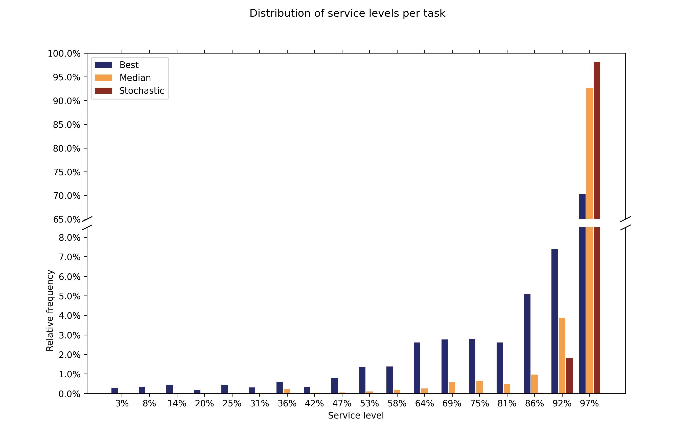
Figure 4: Distribution of service levels

Figure 4 shows the distribution of service levels per task. For this purpose, for each type of travel time, we collected all service levels for each individual task for every instance and plotted their empirical distribution. While stochastic travel times guarantee a service level of at least 90% at all times, median and best-case travel time solutions frequently provide significantly lower values, down to 3% in some cases. Moreover, best-case travel time solutions violate the prescribed minimum service level for 25% of tasks, while for median travel time solutions, this holds in around 8% of cases. This emphasizes the unpredictability of minimum service levels when deterministic travel times are assumed, which ultimately has a significant impact on perceived service quality. Hence, explicitly considering stochastic travel times in the problem formulation yields solutions that seldom violate any time windows, resulting in a high and reliable quality of service.

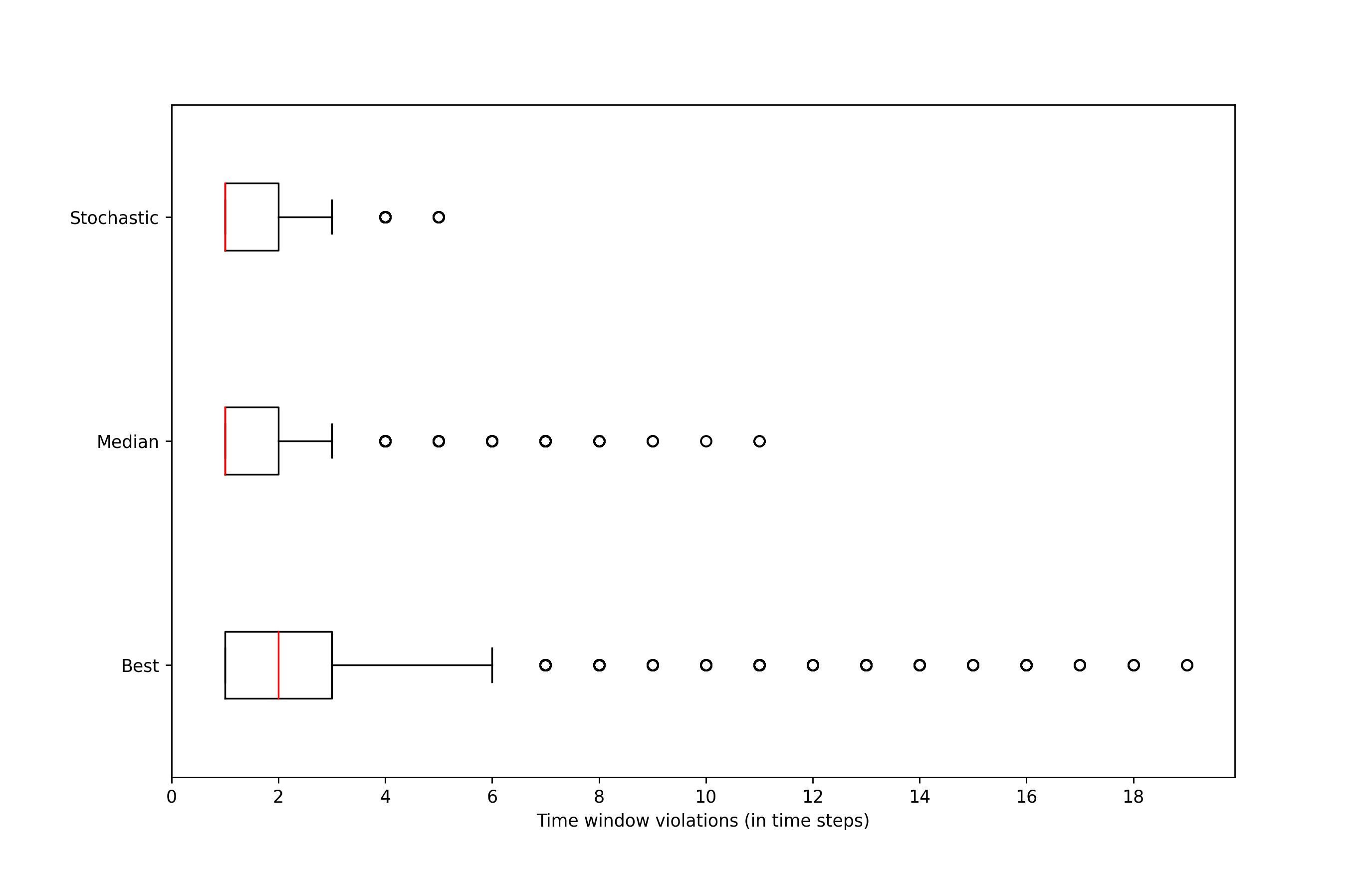
Figure 5: Frequency of durations of time window violations

Figure 5 visualizes the occurrence of time window violations, measured in time steps. Recall that for our purposes, each time step is 2 minutes long. As for Figure 4, we collected all potential time window violations and their lengths for each instance and each scenario. Overall, best-case travel time solutions have higher median time window violations, larger 75%-quantiles, and more outliers than stochastic solutions. At the same time, the median time window violations and 75%-quantiles of median and stochastic solutions are almost identical. Nevertheless, the former solutions exhibit far more large delays, reaching up to 11 time steps, i.e., 22 minutes. In total, assuming deterministic travel times usually returns solutions that cause comparably long delays, are at risk of delaying tasks by significant amounts, and lead to highly volatile delays, which are several magnitudes larger than the maximum acceptable delay $LF_{i}^{e}-LF_{i}$. These effects lead to passengers becoming dissatisfied and baggage handling operators having to pay financial penalties. Using stochastic travel times greatly benefits a solution’s quality in these regards, typically causing few, small delays and ruling out undesirably long delays.
To summarize the above findings, we observe that solutions based on deterministic travel times, be they best-case, median, or worst-case, return strategies that do not live up to the set service quality. Explicitly incorporating stochastic travel times into the model allows for solutions that efficiently use the available workforce to increase safety time buffers, guarantee a stable service level, and prevent large delays.

7 Conclusion

We have examined the problem of forming and routing worker teams, consisting of workers of different hierarchical skill levels. We extended the works of Dall’Olio and Kolisch (2023) by considering stochastic travel times across the apron. For this purpose, we adjusted their MIP formulation to suit stochastic travel times, provide a service level guarantee, and disallow extreme delays for each task. Furthermore, we introduced an alternative master problem formulation abbreviated as DRMP. Moreover, we provided an adjusted dominance rule used to solve the pricing problem associated with said model, allowing us to solve multiple pricing networks at once, at the expense of only a slight increase in runtime. This result ultimately made the usage of said formulation practically feasible. We then combined the DRMP with the formulation proposed by the aforementioned authors to develop a new solution approach based on a Branch-Price-and-Cut approach. More specifically, we switch between two master problem formulations, depending on the characteristics of the current (integer) solution and the position within the branching tree. Furthermore, we introduced an improved branching strategy based on the worst-case finish times of individual tasks, which was able to greatly improve the solution quality and algorithm’s convergence speed. Moreover, we applied an exact separation procedure for rank-1 Chvátal-Gomory cuts and carefully designed the decision process of when and how to separate said cuts. Our computational studies indicate that our proposed algorithm is able to outperform the standard Branch-Price-and-Check approach by Dall’Olio and Kolisch (2023), solving more instances to optimality and significantly reducing optimality gaps. Additionally, we observed that including stochastic travel times into the model is a superior approach to assuming deterministic travel times, as the solutions obtained allow for earlier expected termination of tasks, less frequent and smaller delays, and a guaranteed, stable service level and maximum possible delay.
Our computational studies have shown that the impact of branching on task finish times on upper and lower bounds gradually decreases with increasing problem size. Hence, it might be worthwhile to further analyze the reasons for this phenomenon and identify more advanced branching strategies on task time windows that scale well with the problem size. Moreover, one of our core assumptions is the separation of daily flight schedules into segments of 1 to 2 hours, within which optimal decisions can be made without considering what happens before or after this. While this is a realistic assumption for Munich Airport, it might not hold for other airports. In order to derive reasonable team formation and routing decisions for such settings, one might consider an infinite time horizon, potentially applying online optimization techniques. Moreover, as we consider task execution times and time windows to be deterministic, our model is still a simplification. As the exact solvability of a full-fledged stochastic model that incorporates all potential factors of stochasticity is questionable, further advances toward heuristic approaches can be made. For instance, the order in which the pricing networks are solved in each pricing step has a large impact on the algorithm’s runtime. Moreover, pricing networks can be solved heuristically, potentially returning a very good, yet not optimal column, in a fraction of the runtime needed by an exact labeling approach. Such decision processes could be further improved by applying machine learning techniques tailored individually to the problem’s structure.

We thank AeroGround GmbH for providing the data and key industry information. Andreas Hagn and Giacomo Dall’Olio have been funded by the Deutsche Forschungsgemeinschaft (DFG, German Research Foundation) - Project number 277991500.

8 List of Symbols

Sets
$\mathcal{Q}$	Set of profiles
$\mathcal{Q}_{i}$	Set of profiles compatible with task $i$
$\mathcal{Q}^{D}$	Set of disaggregated profiles $(q,s)$
$\mathcal{S}$	Set of skill compositions
$\mathcal{S}_{q}$	Set of skill compositions compatible with profile $q$
$\mathcal{I}$	Set of tasks
$\mathcal{I}^{r}$	Set of tasks executed by route $r$
$\hat{\mathcal{I}}_{q}$	Set of tasks that can be executed by profile q including covering
$\mathcal{R}$	Set of feasible team routes for the AMP
$\bar{\mathcal{R}}$	Subset of all feasible team routes $\mathcal{R}$
$\mathcal{R}^{D}$	Set of feasible team routes for the DMP
$\mathcal{K}$	Set of worker skill levels
$\mathcal{T}$	Set of discrete time points
$B_{i,j}$	(finite) support of travel time delays for tasks $i$ and $j$ (or tasks and the depot)
$\Omega$	Set of all possible travel time realizations
$\mathcal{G}$	Set of indices of rank-1 CGCs present at given node
Variables
$\lambda^{r}_{q}$	Binary variable, equals to 1 if feasible team route $(r,q)$ belongs to a solution of the AMP
$\lambda^{r}_{q,s}$	Binary variable, equals to 1 if feasible team route $(r,q,s)$ belongs to a solution of the DMP
$t$	random variable of stochastic travel times
$t_{i,j}$	random variable of stochastic travel times between nodes $i$ and $j$
Input Parameters
$N_{k}^{D}$	Number of available workers with level $k$
$N_{k}$	Number of available workers with at least level $k$
$\xi_{q,k}$	Number of workers with at least level $k$ required by working profile $q$
$d$	Central worker depot
$ES_{i}$	Earliest start time of task $i$
$LF_{i}$	Latest finish time of task $i$
$LF_{i}^{e}$	Extended latest finish time of task $i$
$w_{i}$	Weight of task $i$
$p_{i,q}$	Processing time of task $i$ when undertaken with working profile $q$
$\alpha$	Chance constraint probability (minimum service level requirement)
$t^{det}$	Vector of deterministic, best-case travel times
$\omega$	(single) realization of travel times
$\omega_{max}$	worst-case realization of travel times
$t_{i,j}^{\alpha}$	largest $\alpha$-quantile of the distribution of $t_{i,j}$
Model Parameters
$P_{i}(\cdot)$	Penalty function for time window violations at task $i$
$\mathbb{E}(c^{r})$	Expected cost of route $r$
$tl^{r}$	Leave time from the depot for the team executing route $r$
$tr^{r}$	Return time to the depot for the team executing route $r$
$S^{r,q}_{i}$	(Stochastic) start time of task $i$ in tour $r$ with profile $q$
$F^{r,q}_{i}$	(Stochastic) finish time of task $i$ in tour $r$ with profile $q$
$F^{r,q}_{i}(\omega_{max})$	Worst-case finish time of task $i$ in tour $r$ with profile $q$
$b_{k,t}^{q}(\omega_{max})$	Number of workers with at least level $k$ required by team route $(r,q)$ at time $t$ if $\omega_{max}$ occurs
$\beta_{k,t}^{s}$	Number of workers with skill level $k$ required by team route $(r,q,s)$ at time $t$ if $\omega_{max}$ occurs
$\mu_{i}$	Value of the dual variable associated with task covering constraints
$\delta_{k,t}$	Value of the dual variable associated with workforce constraints
$\psi_{g}$	Value of the dual variable associated with the rank-1 CGC with index $g$

Model Parameters (contd.)
$\mathcal{G}^{q}$	Pricing network in the ARMP for profile $q$
$\mathcal{G}^{q,s}$	Pricing network in the DRMP for disaggregated profile $(q,s)$
$\mathcal{A}^{q}$	Arcs of networks $\mathcal{G}^{q}$ and $\mathcal{G}^{q,s}$
$\mathcal{V}^{q}$	Nodes of networks $\mathcal{G}^{q}$ and $\mathcal{G}^{q,s}$
$W_{i,j}(F_{i}^{P,max})$	dynamic weight of arc $(i,j)$ depending on the worst-case finish time $F_{i}^{P,max}$ of the previous task
$F_{i}^{L,max}$	worst-case finish time of task $i$ in the path associated with label $L$
$u_{i}$	rank-1 CGC coefficient for task constraint associated with task $i$
$u_{k,t}$	rank-1 CGC coefficient for workforce constraint associated with skill level $k$ and time $t$

9 Feasibility Check Model

Without loss of generality, let $(\bar{\lambda}^{r}_{q})_{(r,q)\in\mathcal{R}}$ be an integer solution to the AMP. We define by

$$\bar{\mathcal{R}}\coloneqq\left\{(r,q)\in\mathcal{R}:\ \bar{\lambda}^{r}_{q}=1\right\}$$

the set of selected team routes. Furthermore, we denote by

$$\bar{\mathcal{R}}^{r}_{-} \coloneqq\left\{(\tilde{r},\tilde{q})\in\bar{\mathcal{R}}:\ tr^{\tilde{r}}\leq tl^{r}\right\}$$

$$\bar{\mathcal{R}}^{r}_{+} \coloneqq\left\{(\tilde{r},\tilde{q})\in\bar{\mathcal{R}}:\ tl^{\tilde{r}}\geq tr^{r}\right\}$$

the set of predecessor and successor tours of team route $(r,q)\in\bar{\mathcal{R}}$, respectively. In the following, we will be referring to elements in $\bar{\mathcal{R}}^{r}_{-}$ and $\bar{\mathcal{R}}^{r}_{+}$ solely by their respective route $\tilde{r}$, because the actual profile and skill composition team routes are mostly irrelevant for the considerations to come. Furthermore, let $x_{k}^{r,\tilde{r}}$ be integer variables indicating the number of workers of skill level $k$ that are regrouped from tour $r$ into tour $\tilde{r}$ after $r$ has finished and $\chi_{k}^{r,\tilde{r}}$ be slack variables. Then, the feasibility check is defined as

$$\min \underset{(r,q)\in\bar{\mathcal{R}}}{\sum}\chi_{k}^{o,r}$$ (28)

s.t. $$\underset{\rho\in\bar{\mathcal{R}}^{r}_{-}}{\sum}\ \underset{\kappa=k}{\overset{K}{\sum}}x_{k}^{\rho,r}+\underset{\kappa=k}{\overset{K}{\sum}}x_{k}^{o,r}+\chi_{k}^{o,r}\geq\xi_{q,k}\quad\forall(r,q)\in\bar{\mathcal{R}}\ \forall k\in\mathcal{K}$$ (29)

$$x_{k}^{o,r}+\underset{\rho\in\bar{\mathcal{R}}^{r}_{-}}{\sum}x_{k}^{\rho,r}=x_{k}^{r,o^{\prime}}+\underset{\phi\in\bar{\mathcal{R}}^{r}_{+}}{\sum}x_{k}^{r,\phi}\quad\forall(r,q)\in\bar{\mathcal{R}}\ \forall k\in\mathcal{K}$$ (30)

$$x_{k}^{o,o^{\prime}}+\underset{(r,q)\in\bar{\mathcal{R}}}{\sum}x_{k}^{o,r}=N_{k}^{D}\quad\forall k\in\mathcal{K}$$ (31)

$$x_{k}^{o,o^{\prime}}+\underset{(r,q)\in\bar{\mathcal{R}}}{\sum}x_{k}^{r,o^{\prime}}=N_{k}^{D}\quad\forall k\in\mathcal{K}$$ (32)

$$x_{k}^{r,\phi}\in\mathbb{Z}_{0}\quad\forall(r,q)\in\bar{\mathcal{R}}\ \forall\phi\in\bar{\mathcal{R}^{r}_{+}}\ \forall k\in\mathcal{K}$$ (33)

$$x_{k}^{o,r},x_{k}^{r,o^{\prime}}\in\mathbb{Z}_{0}\quad\forall(r,q)\in\bar{\mathcal{R}}\quad\forall k\in\mathcal{K}$$ (34)

Constraint (29) ensures that each selected tour has enough qualified workers assigned to it. Constraint (30) acts as a worker flow conservation constraint. Constraints (31) and (32) ensure that the existing workforce size is not exceeded and each worker starts and ends their shift at the depot. The objective function (28) aims at minimizing the sum over all slack variables, i.e., the number of additional workers required to make the current solution disaggregated-feasible. If this value is greater than 0, the available workforce is not sufficient, therefore the found solution is operationally infeasible. Note that the above model can easily be adjusted to solutions of the DMP by considering disaggregated team routes instead of team routes.

10 DMP Solutions and Feasibility Check

Theorem 10.1

Let $(\bar{\lambda}^{r}_{q,s})_{(r,q,s)\in\mathcal{R}^{D}}$ be an integer solution to the DMP (10)–(13). Then, there exists a solution to the feasibility check (28)–(34) with objective function value 0, i.e., the solution to the DMP passes the feasibility check.

Proof 10.2

Proof. We construct a solution for the feasibility check as follows:

1 for $(r,q,s)\in\mathcal{\bar{R}}$ with $\mathcal{\bar{R}}_{-}=\emptyset$ do

2      for $k\in\mathcal{K}$ do

3            Set $x_{k}^{o,r}\coloneqq s_{q,k}$

4       end for

5      

6 end for

7Define $\mathcal{\bar{R}}_{>0}\coloneqq\left\{(r,q,s)\in\mathcal{\bar{R}}:\ \mathcal{\bar{R}}_{-}\neq\emptyset\right\}$ and sort $\mathcal{\bar{R}}_{>0}$ ascending with respect to leave times $tl^{r}$

8 for $(r,q,s)\in\mathcal{\bar{R}}_{>0}$ do

9       Sort $\mathcal{\bar{R}}^{r}_{-}$ ascending with respect to $tl^{\tilde{r}}$

10       for $k\in\mathcal{K}$ do

11            for $(\tilde{r},\tilde{q},\tilde{s})\in\mathcal{\bar{R}}_{-}^{r}$ do

12                  if $s_{q,k}=\underset{\rho\in\mathcal{\bar{R}}_{-}^{r}}{\sum}x_{k}^{\rho,r}$ holds then

13                        go to step 7

14                   end if

15                  else

16                        set

$$x_{k}^{\tilde{r},r}\coloneqq\min\left\{s_{q,k}-\underset{\rho\in\mathcal{\bar{R}}^{r}_{-}}{\sum}x_{k}^{\rho,\tilde{r}},x_{k}^{o,\tilde{r}}+\underset{\rho\in\mathcal{\bar{R}}_{-}^{\tilde{r}}}{\sum}x_{k}^{\rho,\tilde{r}}-\underset{\phi\in\mathcal{\bar{R}}_{+}^{\tilde{r}}}{\sum}x_{k}^{\tilde{r},\phi}\right\}$$ (35)

17                   end if

18                  

19             end for

20            

21            if $s_{q,k}>\underset{\rho\in\mathcal{\bar{R}}_{-}^{r}}{\sum}x_{k}^{\rho,r}$ holds then

22                   set

$$x_{k}^{o,r}\coloneqq\min\left\{s_{q,k}-\underset{\rho\in\mathcal{\bar{R}}^{r}_{-}}{\sum}x_{k}^{\rho,r},N_{k}^{D}-\underset{(\bar{r},\bar{q},\bar{s})\in\mathcal{\bar{R}}}{\sum}x_{k}^{o,\bar{r}}\right\}$$ (36)

23             end if

24            

25       end for

26      

27 end for

28

29for $(r,q,s)\in\mathcal{\bar{R}}$ do

30      for $k\in\mathcal{K}$ do

31            set $x_{k}^{r,o^{\prime}}\coloneqq x_{k}^{o,r}+\underset{\rho\in\mathcal{\bar{R}}_{-}^{r}}{\sum}x_{k}^{\rho,r}-\underset{\phi\in\mathcal{\bar{R}}_{+}^{r}}{\sum}x_{k}^{r,\phi}$

32       end for

33      

34 end for

35for $k\in\mathcal{K}$ do

36      set $x_{k}^{o,o^{\prime}}\coloneqq N_{k}^{D}-\underset{(r,q,s)\in\mathcal{\bar{R}}}{\sum}x_{k}^{o,r}$

37 end for

Algorithm 1 Construction of a solution for the feasibility check

We now show that the solution obtained from Algorithm 1 satisfies constraints (29)–(34).
We start by considering inequalities (29). Let $(r,q,s)\in\mathcal{\bar{R}}$ be a disaggregated team route and $k\in\mathcal{K}$ be a skill level. Assume that $s_{q,k}=x_{k}^{o,r}+\underset{\rho\in\mathcal{\bar{R}}_{-}^{r}}{\sum}x_{k}^{\rho,r}$ holds. We can then conclude

$$\underset{\kappa=k}{\overset{K}{\sum}}\left(x_{k}^{o,r}+\underset{\rho\in\mathcal{\bar{R}}_{-}^{r}}{\sum}x_{k}^{\rho,r}\right)=\underset{\kappa=k}{\overset{K}{\sum}}s_{q,k}\overset{(\ref{definition_skill_comp_leq})}{\geq}\xi_{q,k}$$

holds and thus, constraint (29) is satisfied. Hence, it is sufficient to show that after executing Algorithm 1,

$$s_{q,k}=x_{k}^{o,r}+\underset{\rho\in\mathcal{\bar{R}}_{-}^{r}}{\sum}x_{k}^{\rho,r}$$ (37)

holds for all $(r,q,s)\in\mathcal{\bar{R}}$ and $k\in\mathcal{K}$.
Let $\mathcal{\bar{R}}_{tl}$ be the ordering of elements in $\mathcal{\bar{R}}$ in which they are treated in Algorithm 1. Practically speaking, the first elements of $\mathcal{\bar{R}}_{tl}$ are equal to all disaggregated team routes without predecessor tours, i.e., all team routes whose inbound worker flow variables $x_{k}^{o,r}$ and $x_{k}^{\rho,r}$ are set in lines 1-4 of Algorithm 1, followed by all routes with at least one predecessor tour, sorted ascending with respect to their depot leave time. We note that, for the satisfaction of (37), only the values of inbound worker flow variables $x_{k}^{o,r}$ and $x_{k}^{\rho,r}$ are relevant. Hence, we can prove the satisfaction of said constraint for all skill levels and disaggregated team routes via induction over the set $\mathcal{\bar{R}}_{tl}$.
Let $(r,q,s)\in\mathcal{\bar{R}}_{tl}$ be the first element in $\mathcal{\bar{R}}_{tl}$. From lines 1-5 of Algorithm 1, we then know that $x_{k}^{o,r}=s_{q,k}$ holds for all $k\in\mathcal{K}$. Therefore, (37) is satisfied. We now assume that (37) is satisfied for all $k\in\mathcal{K}$ and all $(r,q,s)\in\mathcal{\bar{R}}_{tl}$ up to a certain index $i-1$. Let $(r,q,s)\in\mathcal{\bar{R}}_{tl}$ be the $i$-th element in $\mathcal{\bar{R}}_{tl}$. Furthermore, let $k\in\mathcal{K}$ be arbitrary and assume that, after executing loop 8-21 of Algorithm 1, (37) is not satisfied for $(r,q,s)$ and $k$. By construction of the worker flow variables $x_{k}^{o,r}$ and $x_{k}^{\rho,r}$, we then know that

$$s_{q,k}>x_{k}^{o,r}+\underset{\rho\in\mathcal{\bar{R}}_{-}^{r}}{\sum}x_{k}^{\rho,r}$$ (38)

holds. Now, consider the state of Algorithm 1 before executing loop 8-21 for $(r,q,s)$ and $k$. Then, from lines 15 and 19 of Algorithm 1 we know that

$$\underset{\tilde{r}\in\mathcal{\bar{R}}_{-}^{r}}{\sum}\left(x_{k}^{o,\tilde{r}}+\left(\underset{\rho\in\mathcal{\bar{R}}_{-}^{\tilde{r}}}{\sum}x_{k}^{\rho,\tilde{r}}-\underset{\phi\in\mathcal{\bar{R}}_{+}^{\tilde{r}}}{\sum}x_{k}^{\tilde{r},\phi}\right)\right)+\left(N_{k}^{D}-\underset{(\tilde{r},\tilde{q},\tilde{s})\in\mathcal{\bar{R}}}{\sum}x_{k}^{o,\tilde{r}}\right)<s_{q,k}$$ (39)

is satisfied. Additionally, we can reformulate the total available workforce $N_{k}^{D}$ with skill level $k$ as

$$N_{k}^{D}=N_{k}^{D}+\underset{(\tilde{r},\tilde{q},\tilde{s})\in\mathcal{\bar{R}}}{\sum}x_{k}^{o,\tilde{r}}-\underset{(\tilde{r},\tilde{q},\tilde{s})\in\mathcal{\bar{R}}}{\sum}x_{k}^{o,\tilde{r}}=\left(N_{k}^{D}-\underset{(\tilde{r},\tilde{q},\tilde{s})\in\mathcal{\bar{R}}}{\sum}x_{k}^{o,\tilde{r}}\right)+\underset{(\tilde{r},\tilde{q},\tilde{s})\in\mathcal{\bar{R}}}{\sum}x_{k}^{o,\tilde{r}}$$

Moreover, we know that for each $(\tilde{r},\tilde{q},\tilde{s})\in\mathcal{\bar{R}}$ and each predecessor tour $\rho\in\mathcal{\bar{R}}_{-}^{\tilde{r}}$, there exists an $(\bar{r},\bar{q},\bar{s})\in\mathcal{\bar{R}}$ and a successor tour $\phi\in\mathcal{\bar{R}}_{+}^{\bar{r}}$ such that $\tilde{r}=\phi$ and $\bar{r}=\rho$ hold, i.e., worker flow variables between tours cancel each other out. Therefore,

$$\underset{(\tilde{r},\tilde{q},\tilde{s})\in\mathcal{\bar{R}}}{\sum}\left(\underset{\rho\in\mathcal{\bar{R}}_{-}^{\tilde{r}}}{\sum}x_{k}^{\rho,\tilde{r}}-\underset{\phi\in\mathcal{\bar{R}}_{+}^{\tilde{r}}}{\sum}x_{k}^{\tilde{r},\phi}\right)=0$$ (40)

holds. Hence, we conclude

$$N_{k}^{D}=\left(N_{k}^{D}-\underset{(\tilde{r},\tilde{q},\tilde{s})\in\mathcal{\bar{R}}}{\sum}x_{k}^{o,\tilde{r}}\right)+\underset{(\tilde{r},\tilde{q},\tilde{s})\in\mathcal{\bar{R}}}{\sum}\left(x_{k}^{o,\tilde{r}}+\left(\underset{\rho\in\mathcal{\bar{R}}_{-}^{\tilde{r}}}{\sum}x_{k}^{\rho,\tilde{r}}-\underset{\phi\in\mathcal{\bar{R}}_{+}^{\tilde{r}}}{\sum}x_{k}^{\tilde{r},\phi}\right)\right)$$

Moreover, the set $\mathcal{\bar{R}}$ can be partitioned into

$$\mathcal{\bar{R}}=\mathcal{\bar{R}}_{-}^{r}\cup\left\{(\tilde{r},\tilde{q},\tilde{s})\in\mathcal{\bar{R}}:\ tl^{\tilde{r}}\leq tl^{r}\leq tr^{\tilde{r}}\right\}\cup\left\{(\tilde{r},\tilde{q},\tilde{s})\in\mathcal{\bar{R}}:\ tl^{r}<tl^{\tilde{r}}\right\}$$

Because the last set of the above partition has only trivial worker inflow variables $x_{k}^{o,\tilde{r}}$ and $x_{k}^{\rho,\tilde{r}}$ associated with it, we can conclude

$$N_{k}^{D} =\left(N_{k}^{D}-\underset{(\tilde{r},\tilde{q},\tilde{s})\in\mathcal{\bar{R}}}{\sum}x_{k}^{o,\tilde{r}}\right)+\underset{\tilde{r}\in\mathcal{\bar{R}}_{-}^{r}}{\sum}\left(x_{k}^{o,\tilde{r}}+\left(\underset{\rho\in\mathcal{\bar{R}}_{-}^{\tilde{r}}}{\sum}x_{k}^{\rho,\tilde{r}}-\underset{\phi\in\mathcal{\bar{R}}_{+}^{\tilde{r}}}{\sum}x_{k}^{\tilde{r},\phi}\right)\right)+$$

$$+\underset{\tilde{r}:\ tl^{\tilde{r}}\leq tl^{r}\leq tr^{\tilde{r}}}{\sum}\left(x_{k}^{o,\tilde{r}}+\left(\underset{\rho\in\mathcal{\bar{R}}_{-}^{\tilde{r}}}{\sum}x_{k}^{\rho,\tilde{r}}-\underset{\phi\in\mathcal{\bar{R}}_{+}^{\tilde{r}}}{\sum}x_{k}^{\tilde{r},\phi}\right)\right)$$

Using (39) and (12), we then infer

$$N_{k}^{D} \overset{(\ref{proof_not_enough_workers})}{<}s_{q,k}+\underset{\tilde{r}:\ tl^{\tilde{r}}\leq tl^{r}\leq tr^{\tilde{r}}}{\sum}\left(x_{k}^{o,\tilde{r}}+\left(\underset{\rho\in\mathcal{\bar{R}}_{-}^{\tilde{r}}}{\sum}x_{k}^{\rho,\tilde{r}}-\underset{\phi\in\mathcal{\bar{R}}_{+}^{\tilde{r}}}{\sum}x_{k}^{\tilde{r},\phi}\right)\right)\leq s_{q,k}+\underset{\tilde{r}:\ tl^{\tilde{r}}\leq tl^{r}\leq tr^{\tilde{r}}}{\sum}\left(x_{k}^{o,\tilde{r}}+\underset{\rho\in\mathcal{\bar{R}}_{-}^{\tilde{r}}}{\sum}x_{k}^{\rho,\tilde{r}}\right)=$$

$$=s_{q,k}+\underset{\tilde{r}:\ tl^{\tilde{r}}\leq tl^{r}\leq tr^{\tilde{r}}}{\sum}s_{\tilde{q},k}\leq\underset{(\tilde{r},\tilde{q},\tilde{s})\in\mathcal{\bar{R}}}{\sum}\beta_{k,tl^{r}}^{\tilde{s}}(\omega_{max})\overset{(\ref{model:workerconstr_disaggregated_mp})}{\leq}N_{k}^{D}$$

which is a contradiction. Hence, (37) must be satisfied with equality. Therefore, constraint (29) is satisfied for $(r,q,s)$ and $k$.
We now consider constraints (30)–(32). From Loops 23-26 and 28-30, it is clear to see that (30) and (31) are satisfied. Furthermore, we know from (40) and lines 24-26 that

$$\underset{(r,q,s)\in\mathcal{\bar{R}}}{\sum}x_{k}^{r,o^{\prime}}\ \overset{L.24-26}{=}\underset{(r,q,s)\in\mathcal{\bar{R}}}{\sum}\left(x_{k}^{o,r}+\left(\underset{\rho\in\mathcal{\bar{R}}_{-}^{r}}{\sum}x_{k}^{\rho,r}-\underset{\phi\in\mathcal{\bar{R}}_{+}^{r}}{\sum}x_{k}^{r,\phi}\right)\right)\overset{(\ref{proof_tour_flows_zero})}{=}\underset{(r,q,s)\in\mathcal{\bar{R}}}{\sum}x_{k}^{o,r}$$

holds. Because (31) holds, we can therefore infer that (32) is also satisfied.
It is left to show that all worker flow variables are integral and non-negative. Using minima in lines 15 and 19 ensures that

$$x_{k}^{o,\tilde{r}}+\underset{\rho\in\mathcal{\bar{R}}_{-}^{\tilde{r}}}{\sum}x_{k}^{\rho,\tilde{r}}-\underset{\phi\in\mathcal{\bar{R}}_{+}^{\tilde{r}}}{\sum}x_{k}^{\tilde{r},\phi}\geq 0$$

and

$$N_{k}^{D}-\underset{\bar{r},\bar{q},\bar{s}\in\mathcal{\bar{R}}}{\sum}x_{k}^{o,\bar{r}}\geq 0$$

are always satisfied for all $(\tilde{r},\tilde{q},\tilde{s})\in\mathcal{\bar{R}}$. Hence, all variable updates preserve non-negativity and integrality. Therefore, Algorithm 1 returns a feasible solution to the feasibility check with an objective function value of 0.

$\square$

11 Proof of Equivalent Pricing Networks

Lemma 11.1

Let $(q,s)\in\mathcal{Q}^{D}$ be a disaggregated profile. Furthermore, let

$$L\coloneqq\left(tl^{L},v,P^{L},T_{v}^{L,cost},(T_{v,i}^{L,perf})_{i\in\mathcal{\hat{I}}_{q}},F_{v}^{L},F_{v}^{L,max}\right)$$

be a label in $\mathcal{G}^{q,s}$. Then, for any disaggregated profile $(q,\tilde{s})\in\mathcal{Q}^{D}$,

$$\tilde{L}\coloneqq\left(tl^{L},v,P^{L},T_{v}^{\tilde{L},cost},(T_{v,i}^{L,perf})_{i\in\mathcal{\hat{I}}_{q}},F_{v}^{L},F_{v}^{L,max}\right)$$

is a label in $\mathcal{G}^{q,\tilde{s}}$ and $P^{L}$ is a feasible path in $\mathcal{G}^{q,\tilde{s}}$.

References

- Binart et al. (2016) Binart S, Dejax P, Gendreau M, Semet F, 2016 A 2-stage method for a field service routing problem with stochastic travel and service times. Computers & Operations Research 65:64–75.
- Çakırgil, Yücel, and Kuyzu (2020) Çakırgil S, Yücel E, Kuyzu G, 2020 An integrated solution approach for multi-objective, multi-skill workforce scheduling and routing problems. Computers & Operations Research 118:104908.
- Christofides, Mingozzi, and Toth (1981) Christofides N, Mingozzi A, Toth P, 1981 State-space relaxation procedures for the computation of bounds to routing problems. Networks 11(2):145–164.
- Dall’Olio and Kolisch (2023) Dall’Olio G, Kolisch R, 2023 Formation and routing of worker teams for airport ground handling operations: A branch-and-price-and-check approach. Transportation Science 57(5):1231–1251.
- Desaulniers, Lessard, and Hadjar (2008) Desaulniers G, Lessard F, Hadjar A, 2008 Tabu search, partial elementarity, and generalized k-path inequalities for the vehicle routing problem with time windows. Transportation Science 42(3):387–404.